Tracking the variation of entanglement Rényi negativity : an efficient quantum Monte Carlo method

Abstract

Although the entanglement entropy probing novel phases and phase transitions numerically via quantum Monte Carlo (QMC) has achieved huge success in pure ground states of quantum many-body systems, numerical explorations on mixed states remain limited, despite the fact that most real-world systems are non-isolated. Meanwhile, entanglement negativity, as a rarely computable entanglement monotone for mixed states, is significant in characterizing mixed-state entanglement, such as in systems with two disconnected regions, dissipation or at finite temperature. However, efficient numerical approaches are scarce to calculate this quantity in large-scale and high-dimensional systems, especially when we need to access how it varies with certain parameters to study critical behaviors. Within the reweight-annealing frame, we present an accessible and efficient QMC algorithm, which is able to achieve the values as well as tracking the variation of the Rényi version of entanglement negativity on some specified parameter path. Our algorithm makes it feasible to directly study the role that entanglement plays at the critical point and in different phases for mixed states in high dimensions numerically. In addition, this method is accessible and easy to parallelize on computers. Through this method, different intrinsic mechanisms in quantum and thermal criticalities with the same universal class have been revealed clearly through the numerical calculations on Rényi negativity.

Introduction.- The increasing communications between condensed matter physics and quantum information science have significantly deepened our understanding of quantum many-body behaviors. Beyond the conventional Landau-Ginzburg-Wilson framework of symmetry breaking and phase transitions Sachdev (1999); Lifshitz and Pitaevskii (2013), quantum entanglement and other complicated microcosmic degrees of freedom serve as the building blocks in various exotic emergent phenomena Amico et al. (2008a); Laflorencie (2016); Zeng et al. (2019). For a bipartite composite system, the entanglement of its pure ground state can be quantified by the entanglement entropy (EE), which captures universal information of the system including critical behaviors Kallin et al. (2014); Helmes and Wessel (2014); Zhao et al. (2022a, b), continuous symmetry breaking Metlitski and Grover (2011); D’Emidio (2020); Deng et al. (2023); Wang et al. (2024a), the underlying conformal field theory (CFT) Calabrese and Lefevre (2008); Fradkin and Moore (2006); Casini and Huerta (2007); Ji and Wen (2019); Tang and Zhu (2020) and topological order Kitaev and Preskill (2006); Levin and Wen (2006); Isakov et al. (2011); Nussinov and Ortiz (2009a, b). However, EE fails to be an entanglement measure when we consider the entanglement or non-separablility of a mixed state, which is a common situation in many-body physics such as a finite-temperature Gibbs state, the state with disconnected partitions and open systems Lifshitz and Pitaevskii (2013); Laflorencie (2016); Yan et al. (2018). The quantification of the mixed-state entanglement is difficult both analytically and numerically since most measures for it require a complex optimization over the full Hilbert space Huang (2014); Amico et al. (2008b); Horodecki et al. (2009); Eisert and Plenio (1999).

The entanglement logarithmic negativity, abbreviated as negativity in this paper, is actually a rarely computable entanglement monotone for mixed states we often resort to Vidal and Werner (2002); Plenio (2005); Audenaert et al. (2002); Eisler and Zimborás (2015); Nobili et al. (2016); Bianchini and Castro-Alvaredo (2016); Eisler and Zimborás (2016); Shapourian et al. (2017); Shapourian and Ryu (2019); Sherman et al. (2016a). Given a bipartite composite system $A\cup B$ with quantum state $\rho$, where $A$ and $B$ are the two subsystems, the negativity that quantifies the entanglement between $A$ and $B$ is defined as $\mathcal{E}:=\ln||\rho^{T_{B}}||$, where $T^{B}$ denotes the partial transpose operating on subsystem $B$, and $||\cdot||$ is the trace norm, which sums over all absolute values of the eigenvalues of $\rho^{T_{B}}$. According to the Peres–Horodecki criterion Peres (1996); Horodecki (1997); Simon (2000), a nonzero value of negativity indicates the existence of entanglement, no matter for a pure or mixed state. Though this statement is not true conversely in general, negativity is yet a powerful tool to describe mixed-state entanglement Calabrese et al. (2012, 2013a, 2013b); Kulaxizi et al. (2014); Calabrese et al. (2014); De Nobili et al. (2015); Wichterich et al. (2009); Ruggiero et al. (2016); Javanmard et al. (2018); Lee and Vidal (2013); Castelnovo (2013); Wen et al. (2016a, b); Hart and Castelnovo (2018); Lu and Grover (2020a); Sherman et al. (2016b); Lu et al. (2020); Lu (2024).

Except for the vanilla negativity $\mathcal{E}$, its Rényi version, dubbed the Rényi negativity (RN), is also a quantity we often consider for mixed states, which is defined as $R_{n}:=-\ln\{{\text{tr}[(\rho^{T_{B}})^{n}]}/{\text{tr}(\rho^{n})}\}$, where $n>1$ is an integer Wu et al. (2020a); Wybo et al. (2020); Wang and Xu (2023); Fan et al. (2024). This definition origins from the replica trick used in analytical studies, where they define $\mathcal{E}_{n_{e}}:=\text{tr}[(\rho^{T_{2}})^{n_{e}}]$ and $\mathcal{E}_{n_{o}}:=\text{tr}[(\rho^{T_{2}})^{n_{o}}]$ with $n_{e}$ and $n_{o}$ denoting the even and odd integer, respectively Calabrese et al. (2012, 2013a, 2013b). Then an analytical continuation will recover $\mathcal{E}_{n_{e}}$ to $\mathcal{E}$ by setting $n_{e}\to 1$. Different from $\mathcal{E}$, $R_{n}$ is not a monotone since it may increase under local operations and classical communications Wybo et al. (2020). Nevertheless, RN can reflect many important properties of entanglement just as $\mathcal{E}$. For instance, it obeys the area law and the area law coefficient is singular at the finite temperature critical point Lu and Grover (2019, 2020b); Wu et al. (2020a); Wang and Xu (2023). Most importantly, it is much easier to calculate it in quantum many-body systems either theoretically or numerically, similar as the relation between Rényi EE and Von Nuemann EE.

In recent years, some numerical approaches have been utilized to calculate RN or negativity Sherman et al. (2016a); Shim et al. (2018); Chung et al. (2014a); Wu et al. (2020a); Wang and Xu (2023), while efficient algorithms to compute the variations of them in large-scale and high-dimensional systems are scarce. Especially, for large-scale interacting spin/boson systems, there are few Quantum Monte Carlo (QMC) works Chung et al. (2014b); Wu et al. (2020b), mainly because the incremental trick commonly used in calculating Rényi EE Hastings et al. (2010); Humeniuk and Roscilde (2012); D’Emidio (2020) becomes much more complex and difficult in the case of RN since the lowest order of nontrivial RN is third and the boundary condition of imaginary time is twisted Wu et al. (2020a). It is an important but challenging target to develop an effective QMC extracting RN with high precision and low technical barrier, and many important problems regarding mixed-state entanglement are still blank due to the absence of efficient algorithms.

In this paper, we present an efficient and effective QMC algorithm for RN within the reweight-annealing frame Ding et al. (2024); Wang et al. (2024b). The specific incremental trick (also called the annealing scheme in this paper) we proposed here does not require altering the entangled regions during the simulations. This makes it both accessible with a low technical barrier and capable of delivering high precision. Moreover, the algorithm can naturally achieve the values of RN at different parameter points on a full trajectory in the parameter space, and it is easy for parallelization on computers. With this algorithm, we are able to track the variation of RN with our interested parameter, which is significant for studying many-body entanglements in different phases and to see how thermal and quantum fluctuations engage in the corresponding phase transitions. For example, we demonstrate that quantum mechanism plays totally different roles in the Ising phase transitions of the 1D transverse field Ising model (by tuning the strength of the transverse fields) and the 2D transverse field Ising model (by tuning the temperature with weak transverse fields) even they share the same universality class.

Basic idea.- For convenience, we define two generalized partition functions

$$Z_{n}:=\text{tr}(\rho^{n}),\quad Z_{n}^{T_{B}}:=\text{tr}[(\rho^{T_{B}})^{n}],$$ (1)

which correspond to two types of manifolds (the case that $n=3$ is shown in Fig. 1) in the language of path integral, and ${R}_{n}=-\ln Z_{n}^{T_{B}}/Z_{n}$. Notice that here $\rho:=e^{-\beta H}$ is not normalized in the language of QMC.

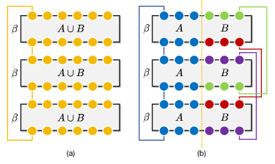
Figure 1: The horizontal axis for the space spins (circles) and the vertical axis for imaginary time. Spins with a same color are connected (glued) along the imaginary time by straight lines with the same color. (a) Manifold for $Z_{3}$, where the three replicas are sequentially connected along the imaginary time direction. It is equivalent to the standard partition function $Z=\text{tr}(\rho)$ but with inverse temperature equal to $3\beta$; (b) manifold for $Z_{n}^{T_{B}}$. The connections among three replicas in subsystem $A$ (the blue part) are exactly same with the left figure. For subsystem $B$, the connections are not in sequence due to the operation $T_{B}$.

Certainly, $Z_{n}^{T_{B}}$, $Z_{n}$ and ${R}_{n}$ are functions of some real parameter $\lambda>0$ (e.g., temperature or the parameter of Hamiltonian), then our starting point is to consider the difference of $R_{n}$ at two different parameter points $\lambda^{\prime}$ and $\lambda^{\prime\prime}$ ($\lambda^{\prime}<\lambda^{\prime\prime}$), i.e.

$$\begin{split}{R}_{n}(\lambda^{\prime\prime})-{R}_{n}(\lambda^{\prime})=&\ln\frac{Z_{n}^{T_{B}}(\lambda^{\prime})}{Z_{n}^{T_{B}}(\lambda^{\prime\prime})}-\ln\frac{Z_{n}(\lambda^{\prime})}{Z_{n}(\lambda^{\prime\prime})}.\end{split}$$ (2)

The ratio $[Z_{n}^{T_{B}}(\lambda^{\prime})/Z^{T_{B}}_{n}(\lambda^{\prime\prime})]$ in Eq. (2) can be further interpreted as a reweighting operation Ferrenberg and Swendsen (1988, 1989); Troyer et al. (2004). To be specific, if we write $Z_{n}^{T_{B}}(\lambda)=\sum_{i}W_{i}(\lambda)$, where $\{W_{i}(\lambda)\}$ are the weights, then the ratio of two partition functions can be assembled by averaging the weight ratios since $Z_{n}^{T_{B}}(\lambda^{\prime})/Z^{T_{B}}_{n}(\lambda^{\prime\prime})=\langle W(\lambda^{\prime})/W(\lambda^{\prime\prime})\rangle_{Z_{n}^{T_{B}}(\lambda^{\prime\prime})}$ with $W(\lambda)\in\{W_{i}(\lambda)\}$ and the sampling is on $Z_{n}^{T_{B}}(\lambda^{\prime\prime})$. The specific form of the estimator $\langle W(\lambda^{\prime})/W(\lambda^{\prime\prime})\rangle_{Z_{n}^{T_{B}}(\lambda^{\prime\prime})}$ depends on the QMC method we use, which transforms the quantum degrees of freedom in $Z_{n}^{T_{B}}(\lambda^{\prime})$ to some classical ones. We take the stochastic series expansion (SSE) method for illustrations in this paper Sandvik (1998, 2003), and the estimators will be introduced later. Similarly, we can discuss $[Z_{n}(\lambda^{\prime})/Z_{n}(\lambda^{\prime\prime})]$. It is worth emphasizing that the view of reweighting here is important because it enables us to estimate the value of $[{R}_{n}(\lambda^{\prime\prime})-{R}_{n}(\lambda^{\prime})]$ from Eq. (2) by estimating the values of $[Z_{n}^{T_{B}}(\lambda^{\prime})/Z^{T_{B}}_{n}(\lambda^{\prime\prime})]$ and $[Z_{n}(\lambda^{\prime})/Z_{n}(\lambda^{\prime\prime})]$ in QMC simulations. Notice that we should save their logarithms in computers to prevent the overflow/underflow problem.

The above procedure is sufficient to derive the relative values of $R(\lambda)$ with different $\lambda^{\prime\prime}$ when we fix $\lambda^{\prime}=\lambda_{0}$, called a reference point, in Eq.(2). Then many behaviors including the position of extreme values and singularities. Further, if we have already known the value of ${R}_{n}(\lambda_{0})$, then the exact values of ${R}_{n}(\lambda)$ can be achieved. In most cases, such a $\lambda_{0}$ is not difficult to find. For example, if $\lambda=\beta\equiv 1/T$, which is the inverse temperature, we can take $\beta_{0}=0$. In this situation, the system is completely disordered and all classical and quantum correlations are destroyed, resulting in ${R}_{n}(\beta_{0})=0$. Practically, we take a sufficiently small number such as $\beta_{0}=10^{-8}$ in our simulations, and the adequacy can be checked by considering a smaller one to see whether the result is convergent. Analogously, if $\lambda$ is the coupling strength of the interacting terms in a Hamiltonian related to the entangled boundary, then setting $\lambda_{0}=0$ would make the two subsystem completely independent and we also have ${R}_{n}(\lambda_{0})=0$. Therefore, depending on our choice of $\lambda$, both finite temperature and zero temperature properties of $R_{n}$ can be explored with our algorithm. For illustrative purpose, we now set $\lambda=\beta$, and other choices of $\lambda$ can be similarly discussed. By identifying $\lambda_{0}\equiv\beta_{0}\equiv 0$, Eq. (2) can be reformulated as

$${R}_{n}(\beta)=\ln\frac{Z_{n}^{T_{B}}(0)}{Z_{n}^{T_{B}}(\beta)}-\ln\frac{Z_{n}(0)}{Z_{n}(\beta)}.$$ (3)

Importance sampling and annealing scheme.- Although the ideas of reweighting and reference point above are simple, if $\beta$ is separated far away from $\beta_{0}$ in the parameter space, then the two distributions at $\beta$ and $\beta_{0}$ regarding $Z_{n}^{T_{B}}$ would differ a lot, making the simulations inefficient and a plethora of samples are required. To fix this problem, we divide the interval $[\beta_{0},\beta]$ into $m$ small subintervals, i.e.

$$\begin{split}\ln\frac{Z_{n}^{T_{B}}(0)}{Z_{n}^{T_{B}}(\beta)}=&\sum_{k=1}^{m}\ln\frac{Z_{n}^{T_{B}}(\beta_{k-1})}{Z^{T_{B}}_{n}(\beta_{k})}\\ \ln\frac{Z_{n}(0)}{Z_{n}(\beta)}=&\sum_{k=1}^{m}\ln\frac{Z_{n}(\beta_{k-1})}{Z_{n}(\beta_{k})},\end{split}$$ (4)

where $\beta_{m}\equiv\beta$. As long as $\beta_{k-1}$ and $\beta_{k}$ in Eq. (4) are close enough in the parameter space, the estimation would be efficient due to the guarantee of importance sampling Neal (2001). It can be expected that the efficacy of Eq. (4) relies greatly on how we divide $[\beta_{0},\beta]$, and the computational complexity scales with the number of subintervals we assign. If we use some crude ways such as dividing it into a bulk of equal subintervals or in a geometric progression with an extreme large/small common ratio, it would be difficult to determine the relation between the required number of subintervals and the system size. These ways are not economic since for a given precision, the required density of the subintervals should be different in different parameter regions.

To approach the problem, we adopt the annealing scheme, which requires polynomial number of subintervals and has shown great performance in practical calculations of partition functions Ding et al. (2024). The key idea is to approximately restrict $[Z_{n}^{T_{B}}(\beta_{k-1})/Z^{T_{B}}_{n}(\beta_{k})]$ and $[Z_{n}(\beta_{k-1})/Z_{n}(\beta_{k})]$ to be some constant $\epsilon<1$ which is close to one for all sizes and $\beta_{k}$ so that the importance samplings are ensured. With some algebras, we can derive that the total number of subintervals $F(L)$ is around $F(L)=(\beta-\beta_{0})\Lambda nL^{d}/|\ln\epsilon|$, where $d$ is the system dimension, $L$ is the length of system and $\Lambda$ is another constant related to the energy density. In fact, an incorrect choice of $\Lambda$ will just effectively change the value of $\epsilon$, thus $\epsilon$ is the only hyperparameter we have to set in this dividing scheme. Similarly, one can discuss when $\lambda$ is some other parameter in the Hamiltonian, and the division number also scales polynomially with the system size. More details about the scheme including the derivation of $F(L)$ can be found in the supplemental materials.

Estimators and models.- In this paper, we focus the SSE method Sandvik (1998, 2003); Yan et al. (2019); Yan (2022), and other QMC methods can be similarly discussed in principle. If $\lambda=\beta$, the estimators for $[Z_{n}^{T_{B}}(\beta_{k-1})/Z^{T_{B}}_{n}(\beta_{k})]$ and $[Z_{n}(\beta_{k-1})/Z_{n}(\beta_{k})]$ are universal as long as the model is sign-problem free. For a given Hamiltonian $H$ and $\rho=e^{-\beta H}$, we have

$$\begin{split}Z_{n}^{T_{B}}(\beta_{k-1})=&\text{tr}(\{\rho^{T_{B}}\}^{n})\\ =&\text{tr}\Bigg{(}\bigg{\{}\bigg{[}\sum_{s=0}^{\infty}\frac{\beta^{s}_{k-1}}{s!}(-H)^{s}\bigg{]}^{T_{B}}\bigg{\}}^{n}\Bigg{)}\\ =&\text{tr}\Bigg{(}\bigg{\{}\bigg{[}\sum_{s=0}^{\infty}\bigg{(}\frac{\beta_{k-1}}{\beta_{k}}\bigg{)}^{s}\frac{\beta^{s}_{k}}{s!}(-H)^{s}\bigg{]}^{T_{B}}\bigg{\}}^{n}\Bigg{)},\\ \end{split}$$ (5)

where $s$ is the order of Taylor expansion, i.e., the total number of non-identity operators of the SSE configuration. Therefore, following the standard procedure of SSE, we can finally obtain

$$\frac{Z_{n}^{T_{B}}(\beta_{k-1})}{Z_{n}^{T_{B}}(\beta_{k})}=\Bigg{\langle}\bigg{(}\frac{\beta_{k-1}}{\beta_{k}}\bigg{)}^{s}\Bigg{\rangle}_{Z_{n}^{T_{B}}(\beta_{k})},$$ (6)

where $\langle...\rangle_{Z_{n}^{T_{B}}(\beta_{k})}$ means that the sampling is performed on $Z_{n}^{T_{B}}(\beta_{k})$. Similarly,

$$\frac{Z_{n}(\beta_{k-1})}{Z_{n}(\beta_{k})}=\Bigg{\langle}\bigg{(}\frac{\beta_{k-1}}{\beta_{k}}\bigg{)}^{s}\Bigg{\rangle}_{Z_{n}({\beta_{k}})}$$ (7)

As mentioned before, if $\lambda$ is a non-temperature parameter, the estimators typically depend on the model. Here we provide an example of the transverse field Ising model (TFIM), whose Hamiltonian is given by

$$H=-\sum_{\langle ij\rangle}Z_{i}Z_{j}-h\sum_{i}X_{i},$$ (8)

where $Z$ and $X$ are Pauli operators with the subscript to label the lattice site they act on, and $\langle ij\rangle$ denotes the nearest neighbor site-pair. Similar to case of temperature, we can derive

$$\frac{Z_{n}^{T_{B}}(h_{k-1})}{Z_{n}^{T_{B}}(h_{k})}=\Bigg{\langle}\bigg{(}\frac{h_{k-1}}{h_{k}}\bigg{)}^{s_{h}}\Bigg{\rangle}_{Z_{n}^{T_{B}}(h_{k})}$$ (9)

$$\frac{Z_{n}(h_{k-1})}{Z_{n}(h_{k})}=\Bigg{\langle}\bigg{(}\frac{h_{k-1}}{h_{k}}\bigg{)}^{s_{h}}\Bigg{\rangle}_{Z_{n}({h_{k}})}$$ (10)

where $s_{h}$ is the number of operators related to the transverse field $h$ only in the series expansions no matter in the manifold $Z_{n}^{T_{B}}(h_{k})$ or $Z_{n}(h_{k})$. The details of the SSE algorithm for TFIM can be found in Ref. Sandvik (2003); Zhou et al. (2022, 2023); Yan et al. (2023).

Example 1: 1D pure state.- We first verify our algorithm on the 1D TFIM chain with length $L$ at zero temperature under periodic boundary condition, and half bipartition is considered. In this case, the state is pure and the behaviors of RN is exactly same as Rényi EE up to a constant factor. Using the estimators in Eq. (9) and Eq. (10), RN can be thus calculated from

$${R}_{n}(h)=\ln\frac{Z_{n}^{T_{B}}(0)}{Z_{n}^{T_{B}}(h)}-\ln\frac{Z_{n}(0)}{Z_{n}(h)}$$ (11)

The reference point $h_{0}$ is taken to be 0 here since a classical state always has no entanglement.

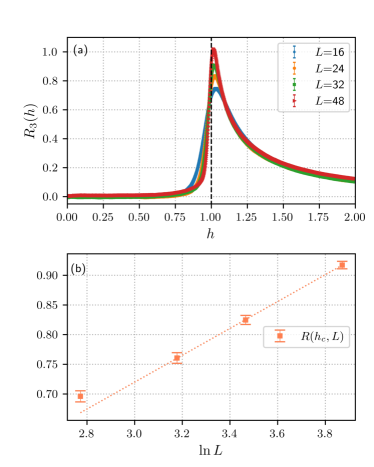
Figure 2: (a) The variation of RN with $h$ in (1+1)D TFIM, where a peak is observed around $h_{c}=1$. (b) The central charge of the underlying conformal field theory at the QCP is fitted to be $c=0.51(3)$, compared with the theoretical prediction that $c=0.5$. The data at $L=16$ is ignored in the fitting, which has great finite-size effect and obviously deviates from the tendency.

In our simulations, we take $n=3$, and calculate the third order RN $R_{3}(h)$ for $L=16,24,32,48$. In Fig. 2(a), we can observe that $R_{3}(h)$ diverges at the quantum critical point (QCP) $h_{c}=1$ when increasing $L$. In addition, since the low energy limit of the critical point is described by $(1+1)$D dimensional conformal field theory, the $R_{n}$ could be completely determined by conformal symmetry as Calabrese et al. (2012, 2013a)

$$R_{n}(h_{c})=\begin{cases}\frac{c}{6}(n-\frac{1}{n})\ln\bigg{(}\frac{L}{\pi a}\sin\frac{\pi l}{L}\bigg{)}+\mathcal{O}(1),&\text{for odd $n$}\\ \frac{c}{3}(\frac{n}{2}-\frac{2}{n})\ln\bigg{(}\frac{L}{\pi a}\sin\frac{\pi l}{L}\bigg{)}+\mathcal{O}(1),&\text{for even $n$}\end{cases}$$ (12)

where $l$ is the length of the subsystem, and the logarithmic negativity is obtained through taking $n\to 1$ within the formula for even $n$. Fitting with Eq. (12), we can extract the value of central charge $c=0.51(3)$, which is consistent with the exact result that $c_{\text{Ising}}=1/2$, shown in Fig. 2(b).

The logarithmic term beyond area law actually reflects that there is long-range entanglement (quantum correlation) at the (1+1)D quantum Ising critical point.

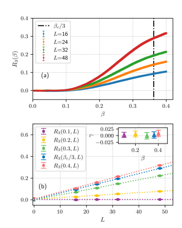
Figure 3: (a) The variation of RN of the 2D TFIM model at $h=2.75$. The dashed line is $1/3$ critical inverse temperature ($\beta_{c}/3$). (b) Linear fittings of the area law behavior of $R_{3}(\beta)$ for $\beta=0.1,0.2,0.3,\beta_{c}/3,0.4$ with data from different sizes. The small panel in the upper right corner shows the values of $\gamma$ fitted at different $\beta$ points, which we consider to be zero within error bars. The colors here label the inverse temperatures.

Example 2: 2D Gibbs state.- For the second example, we consider a 2D TFIM with $h=2.75$, which undergoes a thermal critical point (TCP) that shares the same universality class with the QCP of the (1+1)D TFIM above. However, the former is driven by thermal fluctuations while the latter is driven by quantum fluctuations. The breaking of the area law in Eq. (12) indicates the long-range entanglement at the QCP, which is completely quantum. Correspondingly, we should expect no long-range entanglement in this model, including in the ordered/disordered phase and at the TCP, i.e. we should have the area law behavior $R_{n}=aL-\gamma$ with the nonlocal term $\gamma=0$ for any $\beta$ Lu et al. (2020); Lu and Grover (2020b); Lu (2024).

To verify our expectations, we simulate this model on a torus and under half bipartition without corners. The system sizes are taken to be $L\times(L/2)$ with $L=16,24,32,48$. The TCP of the model is $\beta_{c}=1/T_{c}=1.0874(1)$, and for $R_{3}$, since the three replicas effectively raise the inverse temperature to $3\beta$, relevant critical properties are shifted to $\beta_{c}/3$ or $3T_{c}$ Wu et al. (2020a).

As it shown in Fig. 3(a), $R_{3}$ decays monotonically when lowering $\beta$ (increasing the temperature) and goes to zero at the infinite high temperature. It exhibits no extreme value at the TCP with $\beta=\beta_{c}/3$, different from the peak at QCP shown in Fig. (2)(a) of the 1D model. Fig. 3(b) shows the fitted area laws for $\beta=0.1,0.2,0.3$ (ordered phase), $\beta=\beta_{c}/3$ (TCP), and $\beta=0.4$ (disordered phase). Within the errorbar, $\gamma\sim 0$ in different parameter regions, indicating the absence of long range entanglement even when the phase transition occurs. All of the results accord with the fact that the TCP is classical. Although the statement seems obvious, it was hard to prove before. Moreover, although the RN increases when cooling, which means the quantum property is enhanced, the quantum correlations remain short range ($\gamma\sim 0$). In this sense, the phases beyond or below $T_{c}$ are both trivial for quantum correlation.

Summary and discussions.- Based on the reweight-annealing framework, we have introduced an efficient algorithm with low technical barrier to calculate Rényi negativity with quantum Monte Carlo simulations, which has polynomial computational complexity and is natural to be parallelized on computers. As our algorithm can obtain values of Rényi negativity on a full parameter trajectory in the parameter space, it has great applicability on not only studying how entanglement behaves in different phases and near critical points, but fitting the correction terms in area laws to extract some universal information (central charge, topological order, etc.) of quantum many-body systems. We have verified this in two bipartitioned systems at zero temperature and finite temperature, respectively. The physics of the different intrinsic mechanisms in TCP and QCP of the same universal class have been revealed clearly by our calculations of RN. The generalization to multipartitioned systems is obvious, for which we only need to modify the connections among different replicas.

Acknowledgements.- The authors thank Wei Zhu, Rui-Zhen Huang, Ying-Jer Kao and Tsung-Cheng Lu for helpful discussions. The work is supported by the start-up funding of Westlake University. Z.W. is supported by the China Postdoctoral Science Foundation under Grants No.2024M752898. The authors thank the high-performance computing center of Westlake University and the Beijng PARATERA Tech Co.,Ltd. for providing HPC resources.

Supplemental materials

.1 Annealing scheme ($\lambda=\beta$)

The target of the scheme is to provide an economic way to divide the interval $[\beta_{0},\beta]$ into $m$ subintervals $\{[\beta_{k-1},\beta_{k}]\}$ to ensure the importance sampling, such that we can compute $[Z_{n}^{T_{B}}(\beta_{0})/Z_{n}^{T_{B}}(\beta)]$ and $[Z_{n}(\beta_{0})/Z_{n}(\beta)]$ via

$$\begin{split}&\frac{Z_{n}^{T_{B}}(0)}{Z_{n}^{T_{B}}(\beta)}=\prod_{k=1}^{m}\frac{Z_{n}^{T_{B}}(\beta_{k-1})}{Z^{T_{B}}_{n}(\beta_{k})}\\ &\frac{Z_{n}(0)}{Z_{n}(\beta)}=\prod_{k=1}^{m}\frac{Z_{n}(\beta_{k-1})}{Z_{n}(\beta_{k})}\end{split}$$ (1)

Remember that we have choose the reference point $\beta_{0}\equiv 0$. We mainly focus on $\lambda=\beta$ in this material, and it is similar to discuss $\lambda=h$, where $h$ is the coupling strength of the magnetic fields in the TFIM model. The slight difference will be introduced in the end of the next section.

For a vanilla partition function $Z(\beta)=\text{tr}(e^{-\beta H})$ of some quantum spin model, each classical configuration sampled in SSE simulations is composite of both the states of spins and operators, thus the number of non-identity operators $s_{\text{vn}}$ is exactly some observable in this language, which has the relation $E(\beta)=-\langle s_{\text{vn}}\rangle_{Z(\beta)}/\beta$ with the energy $E(\beta)$. In other words, $\langle s_{\text{vn}}\rangle_{Z(\beta)}\sim\beta|E(\beta)|$.

Suppose $\bar{s}_{\text{tot}}$ and ${s}_{\text{tot}}$ are the corresponding numbers of non-identity operators of $Z^{T_{B}}_{n}(\beta)$ and $Z_{n}(\beta)$. Since $Z_{n}(\beta)=Z(n\beta)$, we directly obtain $\langle s_{\text{tot}}\rangle_{Z_{n}(\beta)}=\langle s_{\text{vn}}\rangle_{Z(n\beta)}\sim n\beta|E(\beta)|$. Then what about $\bar{s}_{\text{tot}}$? In fact, the difference between $\langle\bar{s}_{\text{tot}}\rangle_{Z_{n}^{T_{B}}(\beta^{\prime})}$ and $\langle s_{\text{tot}}\rangle_{Z_{n}(\beta^{\prime})}$, where $\beta^{\prime}\in[\beta_{0},\beta]$, reflects the existence of entanglement because

$$\begin{split}R_{n}(\beta)=&\ln\frac{Z_{n}^{T_{B}}(0)}{Z_{n}^{T_{B}}(\beta)}-\ln\frac{Z_{n}(0)}{Z_{n}(\beta)}\\ =&-\int_{0}^{\beta}d\beta^{\prime}\bigg{[}\frac{d\ln Z_{n}^{T_{B}}(\beta^{\prime})}{d\beta^{\prime}}-\frac{d\ln Z_{n}(\beta^{\prime})}{d\beta^{\prime}}\bigg{]}\\ =&-\int_{0}^{\beta}d\beta^{\prime}\bigg{[}\frac{1}{Z_{n}^{T_{B}}(\beta^{\prime})}\frac{dZ_{n}^{T_{B}}(\beta^{\prime})}{d\beta^{\prime}}-\frac{1}{Z_{n}(\beta^{\prime})}\frac{dZ_{n}(\beta^{\prime})}{d\beta^{\prime}}\bigg{]}\\ =&-\int_{0}^{\beta}d\beta^{\prime}\frac{1}{\beta^{\prime}}\bigg{[}\langle\bar{s}_{\text{tot}}\rangle_{Z_{n}^{T_{B}}(\beta^{\prime})}-\langle s_{\text{tot}}\rangle_{Z_{n}(\beta^{\prime})}\bigg{]}\\ \end{split}$$ (2)

Since the amount of entanglement is an extensive quantity, therefore we should have $\bar{s}_{\text{tot}}\sim n\beta|E(\beta)|$ satisfies as well. With these knowledge, we can now introduce the annealing scheme. We take $[Z_{n}^{T_{B}}(\beta_{k-1})/Z_{n}^{T_{B}}(\beta_{k})]$ for illustrations, and it is similar to discuss $[Z_{n}(\beta_{k-1})/Z(\beta_{k})]$. For brevity, from now, we drop the subscript of $\langle\cdots\rangle$, which should be the corresponding $Z^{T_{B}}_{n}(\beta_{k})$,and write $\bar{s}_{\text{tot}}\equiv s$.

We first require $[Z_{n}^{T_{B}}(\beta_{k-1})/Z_{n}^{T_{B}}(\beta_{k})]=\epsilon<1$ for all $k$, where $\epsilon$ is some constant close to 1 to ensure the importance sampling when estimating $[Z_{n}^{T_{B}}(\beta_{k-1})/Z_{n}^{T_{B}}(\beta_{k})]$ with $\langle(\beta_{k-1}/\beta_{k})^{s}\rangle$ at $\beta_{k}$. If $\epsilon=1$, the two distributions must be exactly the same and this is some trivial reweighting operation. As we mentioned above, $s$ is some observable, therefore we can achieve some estimation $s^{*}$ for it from simulations (same as we measure the energy) at $\beta_{k}$. Hence, we can bring such an $s^{*}$ into

$$\epsilon=\bigg{\langle}\bigg{(}\frac{\beta_{k-1}}{\beta_{k}}\bigg{)}^{s}\bigg{\rangle}\approx\bigg{(}\frac{\beta_{k-1}}{\beta_{k}}\bigg{)}^{s^{*}}.$$ (3)

Eq. (3) enables us to determine the position of $\beta_{k-1}$ only with $\beta_{k}$ since

$$\beta_{k-1}=\epsilon^{1/s^{*}}\beta_{k}$$ (4)

Therefore, if we start from $\beta_{m}$, using Eq. (3), we can determine the rest of $\beta_{m-1},\cdots,\beta_{1}$, and the procedure stops when we encounter some $\beta_{j}$ such that $\beta_{j-1}<\beta_{0}$. Each determination of $\beta_{k-1}$ relys on some simulations on $\beta_{k}$, and in this sense, the inverse temperature gradually goes from $\beta_{m}$ to $\beta_{0}$. This is akin to a standard quantum annealing or thermal annealing process where we tune some parameter, so we call this way of dividing $[\beta_{0},\beta]$ an annealing scheme.

To enable parallelizations, we can manually set the value of $s^{*}$ rather than estimating it from simulations. As energy $E\sim L^{d}$, where $L$ is the system length and $d$ is the dimension, we can set $s^{*}\simeq\Lambda_{k}n\beta_{k}L^{d}$, where $\Lambda_{k}$ is another constant factor related to the energy density. Then, Eq. (4) reduces to

$$\beta_{k-1}=\epsilon^{1/(\Lambda_{k}n\beta_{k}L^{d})}\beta_{k}$$ (5)

If we manually set the value of $\Lambda_{k}$ with some incorrect and uniform $\Lambda$, this would effectively change the true value of $[Z_{n}^{T_{B}}(\beta_{k-1})/Z_{n}^{T_{B}}(\beta_{k})]$ from $\epsilon$, what we set at the beginning, to some other $\epsilon_{k}$. Therefore the dependence on $k$ can be absorbed into the base, i.e.

$$\beta_{k-1}=\epsilon_{k}^{1/(\Lambda n\beta_{k}L^{d})}\beta_{k}$$ (6)

If one preknows the variation of $\Lambda_{k}$ or $\epsilon_{k}$ with $\beta_{k}$, everything would be basically same with that in Eq. (4), but this is not a general case. On another hand, if we further simplify Eq. (6) by setting $\epsilon_{k}\equiv\epsilon$ for all $k$, this operation would just make the value of $[Z_{n}^{T_{B}}(\beta_{k-1})/Z_{n}^{T_{B}}(\beta_{k})]$ achieved in simulations varies with different $k$, but usually at the same order of magnitude if no critical point lies within $[\beta_{0},\beta]$. Such a critical point may change the value of $\Lambda_{k}$ sharply near that point. However, our method is not for locating the critical point, which can be obtained by considering some order parameter or dimensionless quantity such as the Binder cumulant. Therefore, we can assume that we know the position of the critical point, and on the two sides of that point, we can adopt different $\epsilon$ to avoid the problem.

To sum up, by manually setting some $\Lambda$, we only have one hyperparameter $\epsilon$ to determine. Smaller $\epsilon$ we choose, more Monte Carlo samples we need to obtain a given precision. However, if $\epsilon$ is too large, the number of divisions $m$ may be huge, making the total computational resources unaffordable. This means we need some tradeoff on choosing $\epsilon$. Actually, this is not difficult. By doing some trials on small systems, we can obtain some appropriate $\epsilon$ and apply it on larger systems. With this scheme, we can calculate all values of $\beta_{k}$ at the beginning without any simulations, therefore different estimations of $[Z_{n}^{T_{B}}(\beta_{k-1})/Z_{n}^{T_{B}}(\beta_{k})]$ can be parallelized on computers, which are further used to estimate $\ln[Z_{n}^{T_{B}}(\beta_{k-1})/Z_{n}^{T_{B}}(\beta_{k})]$ and $R_{n}(\beta)$.

.2 Analysis of the annealing scheme ($\lambda=\beta$ and $\lambda=h$)

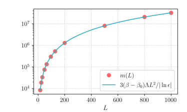
Figure 1: The number of subintervals $m(L)$ with different $L$ (marked in red circles) calculated with the annealing scheme we introduced. It is perfectly in accordance with the function $F(L):=\Lambda n(\beta-\beta_{0})L^{d}/|\ln\epsilon|$, where $n=3$ for the third order of Rényi negativity and $d=2$ for the 2D TFIM model. For example, for $L=48$ (the largest size we simulated), we have $m(48)=74813$ and $F(48)=74804.686$.

For each $\langle(\beta_{k-1}/\beta_{k})^{s}\rangle\approx\epsilon$ close to 1 to ensure the importance sampling, the computational complexity is just as a standard QMC simulation that estimates energy, magnetization, etc, provided the variance of it is finite. Therefore, as long as the annealing scheme we introduce requires polynomial number of subintervals, the total computational complexity is also polynomial. For large $L$, we have

$$\beta_{k-1}=\epsilon^{1/(\Lambda n\beta_{k}L^{d})}\beta_{k}\approx\bigg{(}1+\frac{\ln\epsilon}{\Lambda n\beta_{k}L^{d}}\bigg{)}\beta_{k}$$ (7)

which means

$$\beta_{k}-\beta_{k-1}\approx-\frac{\ln\epsilon}{\Lambda nL^{d}}$$ (8)

thus the total number of subintervals $m=m(L)$ is around $F(L)=(\beta-\beta_{0})\Lambda nL^{d}/|\ln\epsilon|$, which is indeed polynomial. Here we have igored the case when $\beta_{k}$ is small in Eq. (7). This actually contributes little to the value of $m(L)$ because when $\beta_{k}\to 0$, $\epsilon^{1/(\Lambda n\beta_{k}L^{d})}\to 0$ (remember that $\epsilon<1$), making the distribution of $\beta_{k}$ much more sparser than that of the region where $\beta_{k}\gg 0$.

In practical simulations on computers, we cannot really take $\beta_{0}=0$, so we set a sufficiently small number such as $\beta_{0}=10^{-8}$ used in our simulations. The adequacy of the choice of $\beta_{0}$ can be checked by considering a smaller one to see whether the result is convergent. For references, in our simulations of the 2D TFIM model, we take $\Lambda=25h$, $\epsilon=0.1$ and $50$ bins for each $\langle(\beta_{k-1}/\beta_{k})^{s}\rangle$ with $10^{4}$ Monte Carlo steps in each bin. For $\beta=0.362466667\approx\beta_{c}/3$ and $\beta_{0}=10^{-8}$, we calculate the number of subintervals $m(L)$ given by the annealing scheme, which is consistent with our estimation $F(L)=(\beta-\beta_{0})\Lambda nL^{d}/|\ln\epsilon|$, shown in Fig. (1).

Similar discussions can be applied to the case that $\lambda=h$ in the TFIM model, and a modification is just replacing $\beta_{k}$ with $h\beta_{k}$ to estimate $\bar{s}_{h,\text{tot}}$ and $s_{h,\text{tot}}$. We find this hypothetical linear relation actually works well practically and has similar performance as above.

References

- Sachdev (1999) Subir Sachdev, “Quantum phase transitions,” Physics world 12, 33 (1999).
- Lifshitz and Pitaevskii (2013) Evgenii Mikhailovich Lifshitz and Lev Petrovich Pitaevskii, Statistical physics: theory of the condensed state, Vol. 9 (Elsevier, 2013).
- Amico et al. (2008a) Luigi Amico, Rosario Fazio, Andreas Osterloh, and Vlatko Vedral, “Entanglement in many-body systems,” Reviews of modern physics 80, 517–576 (2008a).
- Laflorencie (2016) Nicolas Laflorencie, “Quantum entanglement in condensed matter systems,” Physics Reports 646, 1–59 (2016).
- Zeng et al. (2019) Bei Zeng, Xie Chen, Duan-Lu Zhou, Xiao-Gang Wen, et al., Quantum information meets quantum matter (Springer, 2019).
- Kallin et al. (2014) A. B. Kallin, E. M. Stoudenmire, P. Fendley, R. R. P. Singh, and R. G. Melko, “Corner contribution to the entanglement entropy of an O(3) quantum critical point in 2 + 1 dimensions,” J. Stat. Mech. 2014, 06009 (2014), arXiv:1401.3504 .
- Helmes and Wessel (2014) Johannes Helmes and Stefan Wessel, “Entanglement entropy scaling in the bilayer heisenberg spin system,” Phys. Rev. B 89, 245120 (2014).
- Zhao et al. (2022a) Jiarui Zhao, Yan-Cheng Wang, Zheng Yan, Meng Cheng, and Zi Yang Meng, “Scaling of entanglement entropy at deconfined quantum criticality,” Physical Review Letters 128, 010601 (2022a).
- Zhao et al. (2022b) Jiarui Zhao, Bin-Bin Chen, Yan-Cheng Wang, Zheng Yan, Meng Cheng, and Zi Yang Meng, “Measuring rényi entanglement entropy with high efficiency and precision in quantum monte carlo simulations,” npj Quantum Materials 7, 69 (2022b).
- Metlitski and Grover (2011) Max A Metlitski and Tarun Grover, “Entanglement entropy of systems with spontaneously broken continuous symmetry,” arXiv preprint arXiv:1112.5166 (2011).
- D’Emidio (2020) Jonathan D’Emidio, “Entanglement entropy from nonequilibrium work,” Phys. Rev. Lett. 124, 110602 (2020).
- Deng et al. (2023) Zehui Deng, Lu Liu, Wenan Guo, and HQ Lin, “Improved scaling of the entanglement entropy of quantum antiferromagnetic heisenberg systems,” Physical Review B 108, 125144 (2023).
- Wang et al. (2024a) Zhe Wang, Zhiyan Wang, Yi-Ming Ding, Bin-Bin Mao, and Zheng Yan, “A quantum monte carlo algorithm to extract large-scale data of entanglement entropy and its derivative in high precision,” (2024a), arXiv:2406.05324 [cond-mat.str-el] .
- Calabrese and Lefevre (2008) Pasquale Calabrese and Alexandre Lefevre, “Entanglement spectrum in one-dimensional systems,” Phys. Rev. A 78, 032329 (2008).
- Fradkin and Moore (2006) Eduardo Fradkin and Joel E. Moore, “Entanglement entropy of 2d conformal quantum critical points: Hearing the shape of a quantum drum,” Phys. Rev. Lett. 97, 050404 (2006).
- Casini and Huerta (2007) H. Casini and M. Huerta, “Universal terms for the entanglement entropy in 2+1 dimensions,” Nuclear Physics B 764, 183–201 (2007).
- Ji and Wen (2019) Wenjie Ji and Xiao-Gang Wen, “Noninvertible anomalies and mapping-class-group transformation of anomalous partition functions,” Phys. Rev. Research 1, 033054 (2019).
- Tang and Zhu (2020) Qi-Cheng Tang and Wei Zhu, “Critical scaling behaviors of entanglement spectra,” Chinese Physics Letters 37, 010301 (2020).
- Kitaev and Preskill (2006) Alexei Kitaev and John Preskill, “Topological entanglement entropy,” Phys. Rev. Lett. 96, 110404 (2006).
- Levin and Wen (2006) Michael Levin and Xiao-Gang Wen, “Detecting topological order in a ground state wave function,” Phys. Rev. Lett. 96, 110405 (2006).
- Isakov et al. (2011) Sergei V. Isakov, Matthew B. Hastings, and Roger G. Melko, “Topological entanglement entropy of a bose-hubbard spin liquid,” Nature Physics 7, 772 – 775 (2011).
- Nussinov and Ortiz (2009a) Zohar Nussinov and Gerardo Ortiz, “Sufficient symmetry conditions for Topological Quantum Order,” Proc. Nat. Acad. Sci. 106, 16944–16949 (2009a).
- Nussinov and Ortiz (2009b) Zohar Nussinov and Gerardo Ortiz, “A symmetry principle for topological quantum order,” Annals Phys. 324, 977–1057 (2009b).
- Yan et al. (2018) Zheng Yan, Lode Pollet, Jie Lou, Xiaoqun Wang, Yan Chen, and Zi Cai, “Interacting lattice systems with quantum dissipation: A quantum monte carlo study,” Phys. Rev. B 97, 035148 (2018).
- Huang (2014) Yichen Huang, “Computing quantum discord is np-complete,” New Journal of Physics 16, 033027 (2014).
- Amico et al. (2008b) Luigi Amico, Rosario Fazio, Andreas Osterloh, and Vlatko Vedral, “Entanglement in many-body systems,” Rev. Mod. Phys. 80, 517–576 (2008b).
- Horodecki et al. (2009) Ryszard Horodecki, Paweł Horodecki, Michał Horodecki, and Karol Horodecki, “Quantum entanglement,” Rev. Mod. Phys. 81, 865–942 (2009).
- Eisert and Plenio (1999) Jens Eisert and Martin B Plenio, “A comparison of entanglement measures,” Journal of Modern Optics 46, 145–154 (1999).
- Vidal and Werner (2002) G. Vidal and R. F. Werner, “Computable measure of entanglement,” Phys. Rev. A 65, 032314 (2002).
- Plenio (2005) M. B. Plenio, “Logarithmic negativity: A full entanglement monotone that is not convex,” Phys. Rev. Lett. 95, 090503 (2005).
- Audenaert et al. (2002) K. Audenaert, J. Eisert, M. B. Plenio, and R. F. Werner, “Entanglement properties of the harmonic chain,” Phys. Rev. A 66, 042327 (2002).
- Eisler and Zimborás (2015) Viktor Eisler and Zoltán Zimborás, “On the partial transpose of fermionic gaussian states,” New Journal of Physics 17, 053048 (2015).
- Nobili et al. (2016) Cristiano De Nobili, Andrea Coser, and Erik Tonni, “Entanglement negativity in a two dimensional harmonic lattice: area law and corner contributions,” Journal of Statistical Mechanics: Theory and Experiment 2016, 083102 (2016).
- Bianchini and Castro-Alvaredo (2016) Davide Bianchini and Olalla A. Castro-Alvaredo, “Branch point twist field correlators in the massive free boson theory,” Nuclear Physics B 913, 879–911 (2016).
- Eisler and Zimborás (2016) Viktor Eisler and Zoltán Zimborás, “Entanglement negativity in two-dimensional free lattice models,” Phys. Rev. B 93, 115148 (2016).
- Shapourian et al. (2017) Hassan Shapourian, Ken Shiozaki, and Shinsei Ryu, “Partial time-reversal transformation and entanglement negativity in fermionic systems,” Phys. Rev. B 95, 165101 (2017).
- Shapourian and Ryu (2019) Hassan Shapourian and Shinsei Ryu, “Finite-temperature entanglement negativity of free fermions,” Journal of Statistical Mechanics: Theory and Experiment 2019, 043106 (2019).
- Sherman et al. (2016a) Nicholas E. Sherman, Trithep Devakul, Matthew B. Hastings, and Rajiv R. P. Singh, “Nonzero-temperature entanglement negativity of quantum spin models: Area law, linked cluster expansions, and sudden death,” Phys. Rev. E 93, 022128 (2016a).
- Peres (1996) Asher Peres, “Separability criterion for density matrices,” Physical Review Letters 77, 1413 (1996).
- Horodecki (1997) Pawel Horodecki, “Separability criterion and inseparable mixed states with positive partial transposition,” Physics Letters A 232, 333–339 (1997).
- Simon (2000) R. Simon, “Peres-horodecki separability criterion for continuous variable systems,” Phys. Rev. Lett. 84, 2726–2729 (2000).
- Calabrese et al. (2012) Pasquale Calabrese, John Cardy, and Erik Tonni, “Entanglement negativity in quantum field theory,” Physical review letters 109, 130502 (2012).
- Calabrese et al. (2013a) Pasquale Calabrese, John Cardy, and Erik Tonni, “Entanglement negativity in extended systems: a field theoretical approach,” Journal of Statistical Mechanics: Theory and Experiment 2013, P02008 (2013a).
- Calabrese et al. (2013b) Pasquale Calabrese, Luca Tagliacozzo, and Erik Tonni, “Entanglement negativity in the critical ising chain,” Journal of Statistical Mechanics: Theory and Experiment 2013, P05002 (2013b).
- Kulaxizi et al. (2014) Manuela Kulaxizi, Andrei Parnachev, and Giuseppe Policastro, “Conformal blocks and negativity at large central charge,” Journal of High Energy Physics 2014, 1–25 (2014).
- Calabrese et al. (2014) Pasquale Calabrese, John Cardy, and Erik Tonni, “Finite temperature entanglement negativity in conformal field theory,” Journal of Physics A: Mathematical and Theoretical 48, 015006 (2014).
- De Nobili et al. (2015) Cristiano De Nobili, Andrea Coser, and Erik Tonni, “Entanglement entropy and negativity of disjoint intervals in cft: Some numerical extrapolations,” Journal of Statistical Mechanics: Theory and Experiment 2015, P06021 (2015).
- Wichterich et al. (2009) Hannu Wichterich, Javier Molina-Vilaplana, and Sougato Bose, “Scaling of entanglement between separated blocks in spin chains at criticality,” Physical Review A—Atomic, Molecular, and Optical Physics 80, 010304 (2009).
- Ruggiero et al. (2016) Paola Ruggiero, Vincenzo Alba, and Pasquale Calabrese, “Entanglement negativity in random spin chains,” Physical Review B 94, 035152 (2016).
- Javanmard et al. (2018) Younes Javanmard, Daniele Trapin, Soumya Bera, Jens H Bardarson, and Markus Heyl, “Sharp entanglement thresholds in the logarithmic negativity of disjoint blocks in the transverse-field ising chain,” New Journal of Physics 20, 083032 (2018).
- Lee and Vidal (2013) Yirun Arthur Lee and Guifre Vidal, “Entanglement negativity and topological order,” Physical Review A—Atomic, Molecular, and Optical Physics 88, 042318 (2013).
- Castelnovo (2013) Claudio Castelnovo, “Negativity and topological order in the toric code,” Physical Review A—Atomic, Molecular, and Optical Physics 88, 042319 (2013).
- Wen et al. (2016a) Xueda Wen, Po-Yao Chang, and Shinsei Ryu, “Topological entanglement negativity in chern-simons theories,” Journal of High Energy Physics 2016, 1–30 (2016a).
- Wen et al. (2016b) Xueda Wen, Shunji Matsuura, and Shinsei Ryu, “Edge theory approach to topological entanglement entropy, mutual information, and entanglement negativity in chern-simons theories,” Physical Review B 93, 245140 (2016b).
- Hart and Castelnovo (2018) Oliver Hart and Claudio Castelnovo, “Entanglement negativity and sudden death in the toric code at finite temperature,” Physical Review B 97, 144410 (2018).
- Lu and Grover (2020a) Tsung-Cheng Lu and Tarun Grover, “Structure of quantum entanglement at a finite temperature critical point,” Physical Review Research 2, 043345 (2020a).
- Sherman et al. (2016b) Nicholas E Sherman, Trithep Devakul, Matthew B Hastings, and Rajiv RP Singh, “Nonzero-temperature entanglement negativity of quantum spin models: Area law, linked cluster expansions, and sudden death,” Physical Review E 93, 022128 (2016b).
- Lu et al. (2020) Tsung-Cheng Lu, Timothy H. Hsieh, and Tarun Grover, “Detecting topological order at finite temperature using entanglement negativity,” Phys. Rev. Lett. 125, 116801 (2020).
- Lu (2024) Tsung-Cheng Lu, “Disentangling transitions in topological order induced by boundary decoherence,” (2024), arXiv:2404.06514 .
- Wu et al. (2020a) Kai-Hsin Wu, Tsung-Cheng Lu, Chia-Min Chung, Ying-Jer Kao, and Tarun Grover, “Entanglement renyi negativity across a finite temperature transition: A monte carlo study,” Phys. Rev. Lett. 125, 140603 (2020a).
- Wybo et al. (2020) Elisabeth Wybo, Michael Knap, and Frank Pollmann, “Entanglement dynamics of a many-body localized system coupled to a bath,” Phys. Rev. B 102, 064304 (2020).
- Wang and Xu (2023) Fo-Hong Wang and Xiao Yan Xu, “Entanglement rényi negativity of interacting fermions from quantum monte carlo simulations,” (2023), arXiv:2312.14155 .
- Fan et al. (2024) Ruihua Fan, Yimu Bao, Ehud Altman, and Ashvin Vishwanath, “Diagnostics of mixed-state topological order and breakdown of quantum memory,” PRX Quantum 5, 020343 (2024).
- Lu and Grover (2019) Tsung-Cheng Lu and Tarun Grover, “Singularity in entanglement negativity across finite-temperature phase transitions,” Phys. Rev. B 99, 075157 (2019).
- Lu and Grover (2020b) Tsung-Cheng Lu and Tarun Grover, “Structure of quantum entanglement at a finite temperature critical point,” Phys. Rev. Res. 2, 043345 (2020b).
- Shim et al. (2018) Jeongmin Shim, H.-S. Sim, and Seung-Sup B. Lee, “Numerical renormalization group method for entanglement negativity at finite temperature,” Phys. Rev. B 97, 155123 (2018).
- Chung et al. (2014a) Chia-Min Chung, Vincenzo Alba, Lars Bonnes, Pochung Chen, and Andreas M. Läuchli, “Entanglement negativity via the replica trick: A quantum monte carlo approach,” Phys. Rev. B 90, 064401 (2014a).
- Chung et al. (2014b) Chia-Min Chung, Lars Bonnes, Pochung Chen, and Andreas M. Läuchli, “Entanglement spectroscopy using quantum monte carlo,” Phys. Rev. B 89, 195147 (2014b).
- Wu et al. (2020b) Kai-Hsin Wu, Tsung-Cheng Lu, Chia-Min Chung, Ying-Jer Kao, and Tarun Grover, “Entanglement renyi negativity across a finite temperature transition: a monte carlo study,” Physical Review Letters 125, 140603 (2020b).
- Hastings et al. (2010) Matthew B. Hastings, Iván González, Ann B. Kallin, and Roger G. Melko, “Measuring renyi entanglement entropy in quantum monte carlo simulations,” Phys. Rev. Lett. 104, 157201 (2010).
- Humeniuk and Roscilde (2012) Stephan Humeniuk and Tommaso Roscilde, “Quantum monte carlo calculation of entanglement rényi entropies for generic quantum systems,” Phys. Rev. B 86, 235116 (2012).
- Ding et al. (2024) Yi-Ming Ding, Jun-Song Sun, Nvsen Ma, Gaopei Pan, Chen Cheng, and Zheng Yan, “Reweight-annealing method for calculating the value of partition function via quantum monte carlo,” (2024), arXiv:2403.08642 .
- Wang et al. (2024b) Zhe Wang, Zhiyan Wang, Yi-Ming Ding, Bin-Bin Mao, and Zheng Yan, “Bipartite reweight-annealing algorithm to extract large-scale data of entanglement entropy and its derivative in high precision,” (2024b), arXiv:2406.05324 .
- Ferrenberg and Swendsen (1988) Alan M. Ferrenberg and Robert H. Swendsen, “New monte carlo technique for studying phase transitions,” Phys. Rev. Lett. 61, 2635–2638 (1988).
- Ferrenberg and Swendsen (1989) Alan M. Ferrenberg and Robert H. Swendsen, “Optimized monte carlo data analysis,” Phys. Rev. Lett. 63, 1195–1198 (1989).
- Troyer et al. (2004) Matthias Troyer, Fabien Alet, and Stefan Wessel, “Histogram methods for quantum systems: from reweighting to wang-landau sampling,” Brazilian Journal of Physics 34 (2004), 10.1590/s0103-97332004000300008.
- Sandvik (1998) Anders W. Sandvik, “Stochastic method for analytic continuation of quantum monte carlo data,” Phys. Rev. B 57, 10287–10290 (1998).
- Sandvik (2003) Anders W Sandvik, “Stochastic series expansion method for quantum ising models with arbitrary interactions,” Physical Review E 68, 056701 (2003).
- Neal (2001) Radford M Neal, “Annealed importance sampling,” Statistics and computing 11, 125–139 (2001).
- Yan et al. (2019) Zheng Yan, Yongzheng Wu, Chenrong Liu, Olav F Syljuåsen, Jie Lou, and Yan Chen, “Sweeping cluster algorithm for quantum spin systems with strong geometric restrictions,” Physical Review B 99, 165135 (2019).
- Yan (2022) Zheng Yan, “Global scheme of sweeping cluster algorithm to sample among topological sectors,” Phys. Rev. B 105, 184432 (2022).
- Zhou et al. (2022) Zheng Zhou, Changle Liu, Zheng Yan, Yan Chen, and Xue-Feng Zhang, “Quantum dynamics of topological strings in a frustrated ising antiferromagnet,” npj Quantum Materials 7, 60 (2022).
- Zhou et al. (2023) Zheng Zhou, Changle Liu, Dong-Xu Liu, Zheng Yan, Yan Chen, and Xue-Feng Zhang, “Quantum tricriticality of incommensurate phase induced by quantum strings in frustrated Ising magnetism,” SciPost Phys. 14, 037 (2023).
- Yan et al. (2023) Zheng Yan, Zheng Zhou, Yan-Hua Zhou, Yan-Cheng Wang, Xingze Qiu, Zi Yang Meng, and Xue-Feng Zhang, “Quantum optimization within lattice gauge theory model on a quantum simulator,” npj Quantum Information 9, 89 (2023).