Multiple rescattering effects in the hard knockout reaction ²H$\boldsymbol{(p,2p)n}$

Abstract

The interaction of a proton with a deuteron is the simplest nuclear reaction. However, it allows the study of precursors of nuclear medium effects such as initial-state/final-state interactions (ISI/FSI). In case of hard proton knockout, the deviation of ISI/FSI from the ’standard’ values may carry a signal of color transparency. In this regard, it is important to define the ’standard’ as precisely as possible. This work continues previous studies within the framework of the Generalized Eikonal Approximation (GEA). The focus is on processes where the participating protons experience multiple soft rescattering on the spectator neutron. It is shown that correct treatment of deviations of the trajectories of outgoing protons from the longitudinal direction leads to a significant modification of partial amplitudes with soft rescattering of two outgoing protons and non-vanishing amplitudes with rescattering of incoming and outgoing protons. The new treatment of multiple rescattering is important in kinematics with a forward spectator neutron.

1 Introduction

The quantum-mechanical description of multiple scattering processes is an extremely complex theoretical problem. For high-energy projectiles, the Glauber approximation is applicable Glauber (1959); Glauber and Matthiae (1970), which has proven to be quite effective. The diagrammatic formulation of the multiple scattering theory was given by Gribov Gribov (1969) and Bertocchi Bertocchi (1972). At moderately relativistic energies, this formulation allowed the derivation of the Glauber formalism and, in addition, a more accurate theoretical approach called the Generalized Eikonal Approximation (GEA) Frankfurt et al. (1997a, b); Sargsian (2001); Larionov et al. (2014). The GEA formalism was applied to the hard $A(e,e^{\prime}N)(A-1)^{*}$ and $d(e,e^{\prime}p)n$ reactions, when the energy transfer to the nucleus $\>\stackrel{{\scriptstyle\textstyle>}}{{\sim}}\>$ several GeV Frankfurt et al. (1997a); Sargsian (2001); Boeglin and Sargsian (2024), and the hard $d(p,2p)n$ Frankfurt et al. (1997b); Larionov (2023), $A(\bar{p},\chi_{c})(A-1)^{*}$ Larionov et al. (2014), $d(\bar{p},J/\psi)n$ and $d(\bar{p},\psi^{\prime})n$ Larionov et al. (2019), and $d(\bar{p},\pi^{-}\pi^{0})p$ Larionov and Strikman (2020); Larionov (2022) reactions induced by incoming (anti)protons at similar energies. In such reactions, particles produced in a hard collision with a target nucleon are emitted at small polar angles in the rest frame of the target nucleus, which allows to significantly simplify calculations.

The authors of Ref. Frankfurt et al. (1997b) proposed a GEA-based model for the large-angle $d(p,2p)n$ process and evaluated the effects of color transparency (CT) on the nuclear transparency at $p_{\rm lab}=6-20$ GeV/c. The model of Ref. Frankfurt et al. (1997b) includes single and double soft rescattering diagrams. The transverse momentum transfers in soft elastic $pn$ amplitudes were calculated with respect to the incoming proton beam direction $z$, which allowed the authors to linearize the fast particles propagators with respect to the momentum transfers along $z$. In coordinate space, this resulted in the ordering of the $z$-coordinates of the proton and neutron in the deuteron according to the order of the scattering processes in a given partial amplitude. (This leads, in particular, to the disappearance of partial amplitudes with rescattering of the incoming and outgoing protons, see Fig. 1e,f in Ref. Frankfurt et al. (1997b).). At high beam momenta this is a natural assumption. However, as the beam momentum decreases, its validity becomes questionable due to the large polar scattering angles in the laboratory system.

In Ref. Larionov (2023), the process $d(p,2p)n$ was considered in a broader beam momentum range $p_{\rm lab}=6-75$ GeV/c. The soft momentum transfers in the single rescattering diagrams were calculated relative to the actual directions of the asymptotic momenta of the particles. Accordingly, the positions of the proton and neutron in the deuteron were also ordered along the same directions. However, the calculation of double soft rescattering diagrams was done in the same way as in Ref. Frankfurt et al. (1997b).

In Ref. Larionov (2024), the uncertainties due to the choice of the deuteron wave function (DWF) were studied. It has been shown that at least up to the transverse momentum of the spectator neutron of about 0.4 GeV/c these uncertainties do not sensitively change the nuclear transparency and the tensor analyzing power to influence conclusions on CT.

Another source of uncertainty is the way in which the amplitudes of multiple soft rescattering are treated. Thus, the purpose of the present work is to rederive rescattering amplitudes in the GEA by treating the soft momentum transfers with respect to the actual directions of the asymptotic particle momenta. This leads not only to corrected double rescattering amplitudes when both outgoing protons experience soft rescattering on the spectator neutron, but also to finite amplitudes with rescattering of incoming and outgoing protons, i.e. double- and triple rescattering amplitudes. It is shown that the proper treatment of the geometry of the rescattering process is important for a forward moving spectator, i.e. when the center-of-mass (c.m.) velocity of the colliding $pp$-system is small.

In sec. 2, the GEA model is explained with an accent on new features related to the more precise treatment of the outgoing proton trajectories. The nuclear transparency obtained with the old and new treatment of the multiple scattering is presented in sec. 3. The summary is given in sec. 4.

2 Basic formalism

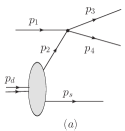
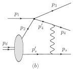
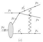
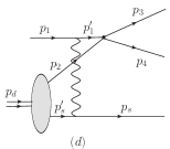
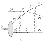
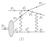
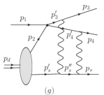
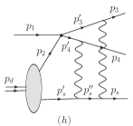
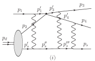
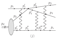
Figure 1: Feynman diagrams for the process $pd\to ppn$ with a slow spectator neutron. The wavy lines denote soft elastic scattering amplitudes. The four-momenta of the deuteron, neutron, beam proton, struck proton, and outgoing protons are denoted as $p_{d}$, $p_{s}$, $p_{1}$, $p_{2}$, $p_{3}$, $p_{4}$, respectively. The primed quantities denote the four-momenta of intermediate particles in the amplitudes with soft rescattering.

Figure 1 shows the partial amplitudes which include the impulse approximation (IA) amplitude and all possible amplitudes with single, double, and triple soft rescattering of the incoming and outgoing protons. The IA amplitude (a) and the amplitudes with single rescattering (b),(c) and (d) have been already calculated in the GEA (see Eqs. (7),(16) and (22) in Ref. Larionov (2023)) and, thus, we start with the double rescattering amplitude (e):

$$M^{(e)} = M_{\rm hard}(p_{3},p_{4},p_{1})\int\frac{d^{4}p_{s}^{\prime\prime}}{(2\pi)^{4}}\int\frac{d^{4}p_{s}^{\prime}}{(2\pi)^{4}}iM_{\rm el}(p_{3},p_{s},p_{3}^{\prime})\frac{i}{p_{3}^{\prime 2}-m^{2}+i\epsilon}$$ (1)

$$\times\frac{i}{p_{1}^{\prime 2}-m^{2}+i\epsilon}\frac{i}{p_{s}^{\prime\prime 2}-m^{2}+i\epsilon}iM_{\rm el}(p_{1}^{\prime},p_{s}^{\prime\prime},p_{1})\frac{i}{p_{s}^{\prime 2}-m^{2}+i\epsilon}\frac{i\Gamma_{d\to pn}(p_{d},p_{s}^{\prime})}{p_{2}^{2}-m^{2}+i\epsilon}~{},$$

where $M_{\rm hard}$ and $M_{\rm el}$ are the invariant amplitudes of the hard and soft elastic scattering, respectively, $m$ is the nucleon mass, and $\Gamma_{d\to pn}$ is the deuteron virtual decay vertex. The hard amplitude is taken out of integrations over internal four-momenta, since this amplitude changes only weakly on the momentum scale of soft rescattering. Neglecting the dependence of the soft rescattering amplitudes on the particle energy (on-shell approximation), we can integrate over the time components of the four-momenta $p_{s}^{\prime}$ and $p_{s}^{\prime\prime}$, closing the integration contours in the lower part of the complex plane, where only the particle poles of the propagators of intermediate spectator contribute. This leads to the following expression:

$$M^{(e)} = M_{\rm hard}(p_{3},p_{4},p_{1})\int\frac{d^{3}k^{\prime\prime}}{(2\pi)^{3}}\int\frac{d^{3}k^{\prime}}{(2\pi)^{3}}iM_{\rm el}(\boldsymbol{k}^{\prime\prime})\frac{i}{p_{3}^{\prime 2}-m^{2}+i\epsilon}$$ (2)

$$\times\frac{i}{p_{1}^{\prime 2}-m^{2}+i\epsilon}\frac{1}{2E_{s}^{\prime\prime}}iM_{\rm el}(\boldsymbol{k}^{\prime})\frac{1}{2E_{s}^{\prime}}\left(\frac{2E_{s}^{\prime}m_{d}}{p_{2}^{0}}\right)^{1/2}(2\pi)^{3/2}\phi(-\boldsymbol{p}_{s}^{\prime})~{},$$

where $\boldsymbol{k}^{\prime}=\boldsymbol{p}_{s}^{\prime\prime}-\boldsymbol{p}_{s}^{\prime}$, $\boldsymbol{k}^{\prime\prime}=\boldsymbol{p}_{s}-\boldsymbol{p}_{s}^{\prime\prime}$ are momentum transfers to the spectator, $E_{s}^{\prime}=\sqrt{\boldsymbol{p}_{s}^{\prime 2}+m^{2}}$ and $E_{s}^{\prime\prime}=\sqrt{\boldsymbol{p}_{s}^{\prime\prime 2}+m^{2}}$ are the on-shell energies of the intermediate spectator. In Eq.(2), we used the relation between the deuteron virtual decay vertex and the DWF, which is applicable in the deuteron rest frame when the spectator four-momentum is on the mass shell (see Ref. Larionov et al. (2018) for derivation):

$$\frac{i\Gamma_{d\to pn}(p_{d},p_{s}^{\prime})}{p_{2}^{2}-m^{2}+i\epsilon}=\left(\frac{2E_{s}^{\prime}m_{d}}{p_{2}^{0}}\right)^{1/2}(2\pi)^{3/2}\phi(-\boldsymbol{p}_{s})~{}.$$ (3)

In the diagrams of Fig. 1, all possible combinations of the intermediate propagators with soft rescattering amplitudes are either of type (a) or type (b) in Fig. 2.

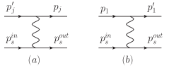
Figure 2: Soft elastic transition amplitudes between the intermediate and asymptotic states for the outgoing protons $j=3,4$ (a) and for the incoming proton 1 (b).

The inverse propagator of intermediate proton related to the transition amplitude of the type (a) in Fig. 2 can be written as

$$p_{j}^{\prime 2}-m^{2}+i\epsilon=2|\boldsymbol{p}_{j}|(p_{s}^{in,\tilde{z}}-p_{s}^{out,\tilde{z}}+\Delta_{j}+i\epsilon)~{},~{}~{}~{}j=3,4~{},$$ (4)

where the $\tilde{z}$-axis is directed along $\boldsymbol{p}_{j}$ and

$$\Delta_{j}\equiv\frac{E_{j}(E_{s}^{out}-E_{s}^{in})}{|\boldsymbol{p}_{j}|}+\frac{(p_{s}^{out}-p_{s}^{in})^{2}}{2|\boldsymbol{p}_{j}|}\simeq\frac{(E_{j}-E_{s}^{in})(E_{s}^{out}-E_{s}^{in})}{|\boldsymbol{p}_{j}|}~{},~{}~{}~{}j=3,4~{}.$$ (5)

In the case of transition amplitude of type (b) in Fig. 2, the inverse propagator of the intermediate proton is expressed as

$$p_{1}^{\prime 2}-m^{2}+i\epsilon=2|\boldsymbol{p}_{1}|(p_{s}^{out,z}-p_{s}^{in,z}-\Delta_{1}+i\epsilon)~{},$$ (6)

where the $z$-axis is directed along the beam momentum $\boldsymbol{p}_{1}$ and

$$\Delta_{1}\equiv\frac{E_{1}(E_{s}^{out}-E_{s}^{in})}{|\boldsymbol{p}_{1}|}-\frac{(p_{s}^{out}-p_{s}^{in})^{2}}{2|\boldsymbol{p}_{1}|}\simeq\frac{(E_{1}+E_{s}^{in})(E_{s}^{out}-E_{s}^{in})}{|\boldsymbol{p}_{1}|}~{}.$$ (7)

In the second step in Eqs.(5),(7), the term $\pm\boldsymbol{p}_{s}^{in}\boldsymbol{k}/|\boldsymbol{p}_{j}|$ ($\boldsymbol{k}=\boldsymbol{p}_{s}^{out}-\boldsymbol{p}_{s}^{in}$) that changes sign when taking integral over $d^{3}k$ was neglected.

Eqs.(5),(7) include the energies of the incoming and outgoing spectator, $E_{s}^{in}=\sqrt{(\boldsymbol{p}_{s}^{in})^{2}+m^{2}}$ and $E_{s}^{out}=\sqrt{(\boldsymbol{p}_{s}^{out})^{2}+m^{2}}$, which depend on the momenta. The momentum $\boldsymbol{p}_{s}^{in}$ is not fixed by the kinematics of the process and is always an integration variable. So is also $\boldsymbol{p}_{s}^{out}$ unless it is the asymptotic momentum of the spectator. In order to further simplify Eq.(2) and similar formulas for other partial amplitudes of Fig. 1 it is necessary to set some fixed ’effective’ values of the $\Delta$’s in Eqs. (4),(6). This can be done as follows. Suppose, the energy of spectator before rescattering, $E_{s}^{in}$, is known. If the spectator after rescattering is in the asymptotic state then its energy is also known, i.e. $E_{s}^{out}=E_{s}$, and the corresponding $\Delta$ is fully determined by Eq.(5) or Eq.(7). If the spectator after rescattering is still in the intermediate state then its energy can be estimated as

$$E_{s}^{out}=\sqrt{(E_{s}^{in})^{2}+\langle k_{t}^{2}\rangle+\Delta_{j}^{2}}~{},~{}~{}~{}j=1,3,4~{},$$ (8)

where $\langle k_{t}^{2}\rangle=B_{pn}^{-1}(|\boldsymbol{p}_{j}|)$ is the average transverse momentum transfer squared and $B_{pn}(|\boldsymbol{p}_{j}|)$ is the slope parameter of the $pn$ elastic amplitude (see Eq.(39) in Ref. Larionov (2023)). Eq.(8) is obtained neglecting any correlation between momentum of the spectator before rescattering and momentum transfer and setting the longitudinal momentum transfer to satisfy the on-shell condition for the intermediate state of the $j$-th proton. By substituting Eq.(8) in Eqs.(5),(7) and solving the resulting quadratic equation with respect to $\Delta_{j}$ one obtains the following formula:

$$\Delta_{j}=\frac{1}{1-\beta^{2}}\left(E_{s}^{in}\beta-\sqrt{(E_{s}^{in}\beta)^{2}-\langle k_{t}^{2}\rangle(1-\beta^{2})}\right)~{},$$ (9)

where

$$\beta=\left\{\begin{array}[]{ll}|\boldsymbol{p}_{1}|/(E_{1}+E_{s}^{in})&\mbox{~{}~{}for~{}~{}}j=1\\ |\boldsymbol{p}_{j}|/(E_{j}-E_{s}^{in})&\mbox{~{}~{}for~{}~{}}j=3,4~{}.\end{array}\right.$$ (10)

(The choice of the ’-’ sign at the square root in Eq.(9) ensures that $\Delta_{j}$ is finite in the high-energy limit $\beta\to 1$.) The procedure is repeated for the next soft rescattering from left to right in the amplitude by setting the new $E_{s}^{in}$ equal to the previously determined $E_{s}^{out}$. For the first rescattering, $E_{s}^{in}=m$ is set since in this case the spectator momentum is strongly suppressed by the DWF.

Having fixed $\Delta$’s, we can now proceed to simplify Eq.(2). The following relations are used to transfer the propagators and wave functions to the coordinate representation:

$$\frac{i}{p+i\epsilon}=\int dz^{0}\Theta(z^{0})\mbox{e}^{ipz^{0}}~{},$$ (11)

$$(2\pi)^{3/2}\phi(-\boldsymbol{p}_{s}^{\prime})=\int d^{3}r\mbox{e}^{i\boldsymbol{p}_{s}^{\prime}\boldsymbol{r}}\phi(\boldsymbol{r})~{},~{}~{}~{}\boldsymbol{r}=\boldsymbol{r}_{2}-\boldsymbol{r}_{s}~{},$$ (12)

where $\Theta(x)$ is the Heaviside step function. By using relations (4),(6),(11) the propagators can be written as

$$\frac{i}{p_{1}^{\prime 2}-m^{2}+i\epsilon}=\frac{i}{2|\boldsymbol{p}_{1}|(k^{\prime,z}-\Delta_{1}+i\epsilon)}=\frac{1}{2|\boldsymbol{p}_{1}|}\int dz^{0}\Theta(z^{0})\mbox{e}^{i(k^{\prime,z}-\Delta_{1})z^{0}}~{},$$ (13)

$$\frac{i}{p_{3}^{\prime 2}-m^{2}+i\epsilon}=\frac{i}{2|\boldsymbol{p}_{3}|(-k^{\prime\prime,\tilde{z}}+\Delta_{3}+i\epsilon)}=\frac{1}{2|\boldsymbol{p}_{3}|}\int d\tilde{z}^{0}\Theta(\tilde{z}^{0})\mbox{e}^{i(-k^{\prime\prime,\tilde{z}}+\Delta_{3})\tilde{z}^{0}}~{}.$$ (14)

Thus, it is convenient to perform the integrations in the cylindrical coordinates:

$$d^{3}k^{\prime}=d^{2}k_{t}^{\prime}dk^{\prime,z}~{},$$ (15)

$$d^{3}k^{\prime\prime}=d^{2}k_{t}^{\prime\prime}dk^{\prime\prime,\tilde{z}}~{},$$ (16)

where $\boldsymbol{k}_{t}^{\prime}\perp\boldsymbol{e}_{z}\equiv\boldsymbol{p}_{1}/|\boldsymbol{p}_{1}|$, $\boldsymbol{k}_{t}^{\prime\prime}\perp\boldsymbol{e}_{\tilde{z}}\equiv\boldsymbol{p}_{3}/|\boldsymbol{p}_{3}|$. The phase of the integrand in Eq.(12) can be rewritten as

$$\boldsymbol{p}_{s}^{\prime}\boldsymbol{r}=(\boldsymbol{p}_{s}-\boldsymbol{k}^{\prime\prime}-\boldsymbol{k}^{\prime})\boldsymbol{r}=\boldsymbol{p}_{s}\boldsymbol{r}-\boldsymbol{k}_{t}^{\prime\prime}\boldsymbol{\tilde{b}}-k^{\prime\prime,\tilde{z}}\tilde{z}-\boldsymbol{k}_{t}^{\prime}\boldsymbol{b}-k^{\prime,z}z~{},$$ (17)

where $\tilde{z}=\boldsymbol{r}\boldsymbol{e}_{\tilde{z}}$ and $\boldsymbol{\tilde{b}}=\boldsymbol{r}-\tilde{z}\boldsymbol{e}_{\tilde{z}}$ are, respectively, the relative longitudinal and transverse displacements of the nucleons in the deuteron with respect to the $\boldsymbol{e}_{\tilde{z}}$ direction, while $z=\boldsymbol{r}\boldsymbol{e}_{z}$ and $\boldsymbol{b}=\boldsymbol{r}-z\boldsymbol{e}_{z}$ are those with respect to the $\boldsymbol{e}_{z}$ direction. Substituting Eqs.(12)-(17) in Eq.(2) and assuming that the soft elastic $pn$ rescattering amplitudes depend on the transverse momentum transfers only the integrations over longitudinal momentum transfers can be easily performed giving

$$\int\frac{dk^{\prime\prime,\tilde{z}}}{2\pi}\int\frac{dk^{\prime,z}}{2\pi}\mbox{e}^{i(k^{\prime,z}-\Delta_{1})z^{0}+i(-k^{\prime\prime,\tilde{z}}+\Delta_{3})\tilde{z}^{0}-ik^{\prime\prime,\tilde{z}}\tilde{z}-ik^{\prime,z}z}=\delta(z^{0}-z)\delta(\tilde{z}^{0}+\tilde{z})\mbox{e}^{-i\Delta_{1}z-i\Delta_{3}\tilde{z}}~{}.$$ (18)

Integrating over $dz^{0}$ and $d\tilde{z}^{0}$ removes the $\delta$-functions which gives

$$M^{(e)}=2m^{1/2}M_{\rm hard}(p_{3},p_{4},p_{1})\int d^{3}r\Theta(z)\Theta(-\tilde{z})\mbox{e}^{i\boldsymbol{p}_{s}\boldsymbol{r}-i\Delta_{1}z-i\Delta_{3}\tilde{z}}\phi(\boldsymbol{r})\Gamma_{1}(b)\Gamma_{3}(\tilde{b})~{},$$ (19)

where

$$\Gamma_{i}(b)=-\frac{i}{4|\boldsymbol{p}_{i}|m}\int\frac{d^{2}k_{t}}{(2\pi)^{2}}\mbox{e}^{-i\boldsymbol{k}_{t}\boldsymbol{b}}M_{\rm el}(|\boldsymbol{p}_{i}|,k_{t})~{},$$ (20)

with $\boldsymbol{k}_{t}\perp\boldsymbol{p}_{i}$, is the profile function. The integration over azimuthal angle of the transverse momentum transfer $\boldsymbol{k}_{t}$ can be performed analytically which gives

$$\Gamma_{i}(b)=-\frac{i}{8\pi|\boldsymbol{p}_{i}|m}\int\limits_{0}^{+\infty}dk_{t}k_{t}M_{\rm el}(|\boldsymbol{p}_{i}|,k_{t})J_{0}(k_{t}b)~{},$$ (21)

where

$$J_{0}(x)=\frac{1}{2\pi}\int\limits_{0}^{2\pi}d\phi\,\mbox{e}^{-ix\cos\phi}$$ (22)

is the Bessel function of the first kind. In the case of the elastic $pn$ amplitude in the standard high-energy form,

$$M_{\rm el}(p_{\rm lab},k_{t})=2p_{\rm lab}m\sigma_{pn}^{\rm tot}(i+\rho_{\rm pn})\mbox{e}^{-B_{\rm pn}k_{t}^{2}/2}~{},$$ (23)

where $\sigma_{pn}^{\rm tot}$ is the total $pn$ cross section, $\rho_{\rm pn}=\mbox{Re}M_{\rm el}(p_{\rm lab},0)/\mbox{Im}M_{\rm el}(p_{\rm lab},0)$ is the ratio of the real part of the forward $pn$ scattering amplitude to the imaginary one, and $B_{\rm pn}$ is the slope of the dependence on the transverse momentum transfer, the profile function can be expressed as

$$\Gamma_{i}(b)=-\frac{iM_{\rm el}(|\boldsymbol{p}_{i}|,0)}{8\pi|\boldsymbol{p}_{i}|mB_{\rm pn}}\mbox{e}^{-b^{2}/2B_{\rm pn}}~{}.$$ (24)

Equations (20),(21) are applicable also if the CT effects are included via the dependence of the effective $pn$ cross section on the longitudinal distance between proton and neutron in the deuteron (see Eq.(41) in Ref. Larionov (2023)).

The amplitude (f) is obtained from Eq.(19) by replacing $3\to 4$ in all multipliers except the hard amplitude. The latter is asymmetric with respect to the exchange of quantum numbers of the third and fourth protons, which provides the same asymmetry of the total amplitude.

The amplitude (g) can also be obtained in the GEA by explicitly taking into account the different directions of the momenta of incoming and outgoing protons. We will not repeat the derivation which is much similar to that of Eq.(19). The resulting expression is

$$M^{(g)}=2m^{1/2}M_{\rm hard}(p_{3},p_{4},p_{1})\int d^{3}r\Theta(-\tilde{z})\Theta(-\tilde{\tilde{z}})\mbox{e}^{i\boldsymbol{p}_{s}\boldsymbol{r}-i\Delta_{3}\tilde{z}-i\Delta_{4}\tilde{\tilde{z}}}\phi(\boldsymbol{r})\Gamma_{3}(\tilde{b})\Gamma_{4}(\tilde{\tilde{b}})~{}.$$ (25)

The directions of $\tilde{z}$ and $\tilde{\tilde{z}}$ axes are chosen along the momenta $\boldsymbol{p}_{3}$ and $\boldsymbol{p}_{4}$, respectively.

It is also straightforward to calculate the triple rescattering amplitude (i):

$$M^{(i)} = -2m^{1/2}M_{\rm hard}(p_{3},p_{4},p_{1})\int d^{3}r\Theta(z)\Theta(-\tilde{z})\Theta(-\tilde{\tilde{z}})\mbox{e}^{i\boldsymbol{p}_{s}\boldsymbol{r}-i\Delta_{1}z-i\Delta_{3}\tilde{z}-i\Delta_{4}\tilde{\tilde{z}}}\phi(\boldsymbol{r})$$ (26)

$$\times\Gamma_{1}(b)\Gamma_{3}(\tilde{b})\Gamma_{4}(\tilde{\tilde{b}})~{}.$$

The directions of the $\tilde{z}$ and $\tilde{\tilde{z}}$ axes are defined as in Eq.(25). The longitudinal momentum transfers $\Delta_{1},\Delta_{3}$ and $\Delta_{4}$ are calculated using Eqs.(5),(7),(9). The amplitudes (h) and (j) are given by Eq.(25) and Eq.(26), respectively, but with another values of $\Delta_{3}$ and $\Delta_{4}$, determined by using the procedure described above (see Eqs.(5),(9),(10)).

The ladder rescattering diagrams of Fig. 1 are not exhausting the full set of possible diagrams with double and triple rescattering, since the cross-diagrams are not included. For example, one can consider the diagram obtained from (e) by changing the order of rescattering of the protons 1 and 3. However, such diagrams can not be treated as ISI/FSI and, thus, we will not include them. However, there is an infinite set of ladder diagrams with successive rescatterings of protons 3 and 4 on the spectator neutron. For example, one can add rescattering of the proton 3 on the r.h.s of the diagram (g), then rescattering of proton 4 etc. It is possible to show that every new rescattering of the proton 3 or 4 brings, respectively, a factor of $-\Gamma_{3}(\tilde{b})/2$ or $-\Gamma_{4}(\tilde{\tilde{b}})/2$ in Eqs.(25),(26). Here, the factor 1/2 comes from the integral

$$\int\frac{dk^{\tilde{z}}}{2\pi}\frac{i}{-k^{\tilde{z}}+\Delta+i\epsilon}$$ (27)

over longitudinal momentum transfer from the last scattered proton (here 3). Thus, the integrands in Eqs.(25),(26) get multiplied by the factor

$$1-\frac{1}{2}\Gamma_{3}(\tilde{b})+\frac{1}{4}\Gamma_{3}(\tilde{b})\Gamma_{4}(\tilde{\tilde{b}})-\frac{1}{8}\Gamma_{3}(\tilde{b})\Gamma_{4}(\tilde{\tilde{b}})\Gamma_{3}(\tilde{b})+\ldots$$

$$=\frac{1-\frac{1}{2}\Gamma_{3}(\tilde{b})}{1-\frac{1}{4}\Gamma_{3}(\tilde{b})\Gamma_{4}(\tilde{\tilde{b}})}~{}.$$ (28)

(In the case of the amplitudes (h) and (j) the replacement $\Gamma_{3}(\tilde{b})\leftrightarrow\Gamma_{4}(\tilde{\tilde{b}})$ in Eq.(28) should be performed.) The convergence condition of the two geometrical series contributing Eq.(28) is $|\frac{1}{4}\Gamma_{3}(\tilde{b})\Gamma_{4}(\tilde{\tilde{b}})|<1$. We checked in numerical calculations that this condition is well satisfied.

In the high-energy limit, when all particles propagate almost parallel to the beam direction $\boldsymbol{e}_{z}$, $\Theta$-functions in Eq.(19) become mutually excluding and, thus, $M^{(e)}=M^{(f)}=0$ in agreement with Ref. Frankfurt et al. (1997b). Same is of course true for the amplitudes with triple rescattering, i.e. $M^{(i)}=M^{(j)}=0$, as follows from Eq.(26). However, the amplitude (25) does not disappear at high energies as the two $\Theta$-functions simply merge in a single one (see Eq.(32) in Ref. Larionov (2023)). Thus, this amplitude is expected to be the leading rescattering amplitude, in addition to the single rescattering amplitudes.

At moderate energies, when the outgoing protons have some finite transverse momenta, there is a certain region in $\boldsymbol{r}$-space where the products of $\Theta$-functions do not disappear and the amplitudes (19),(26) may become finite. However, in numerical analysis, we did not find any finite contribution of the triple rescattering amplitude (26) in all kinematics, except the cases when one of the protons scatters backward in the deuteron rest frame which is only possible with fast-forward-moving spectator ($\alpha_{s}\raisebox{-2.15277pt}{$\>\stackrel{{\scriptstyle\textstyle<}}{{\sim}}\>$}0.5$ see Eq.(32) below). Since such extreme kinematics requires relativistic corrections to the DWF, we will not discuss it. Thus, only the contributions of the single and double soft rescattering amplitudes will be considered below. Thereby, the renormalization factor, Eq.(28), is taken into account.

3 Numerical analysis

To evaluate the effects of soft rescattering, we will calculate the nuclear transparency which is defined as

$$T=\frac{\overline{|M^{(a)}+M^{(b)}+M^{(c)}+M^{(d)}+\ldots+M^{(j)}|^{2}}}{\overline{|M^{(a)}|^{2}}}~{},$$ (29)

where the numerator is the modulus squared of the sum of all partial amplitudes of Fig. 1, and the denominator is the modulus squared of the IA amplitude. The overline means averaging over spin projections of incoming particles and summation over spin projections of the outgoing particles. The calculation was carried out in the deuteron rest frame with the $z$-axis along the proton momentum. The kinematic variables characterizing the particles in the final state are as follows:

$$t=(p_{1}-p_{3})^{2}$$ (30)

– the square of four-momentum transfer between the incoming proton and one of the two scattered protons;

$$\phi=\phi_{3}-\phi_{s}$$ (31)

– the azimuthal angle between the transverse momentum of the scattered proton for which $t$ is measured and that of the spectator neutron;

$$\alpha_{s}=\frac{2(E_{s}-p_{s}^{z})}{m_{d}}$$ (32)

– the light cone variable defined such that, in the infinite momentum frame with the deuteron moving fast backward, $\alpha_{s}/2$ is the fraction of the deuteron momentum carried by the spectator neutron; $p_{st}$ – the transverse momentum of the neutron. Since, in the absence of particle polarizations, the rotational symmetry about $z$ axis is satisfied, four variables fully characterize the event.

In order to see the influence of the different treatments of the multiple rescattering effects, the $\phi$-dependence of the transparency $T$ was studied at several fixed values of $t$, $\alpha_{s}$ and $p_{st}$, for the proton beam momentum $p_{\rm lab}=4$ and 15 GeV/c. The calculations were performed with and without including the double rescattering amplitudes, i.e. those of Fig. 1e,f,g,h. For comparison, the results with the older treatment of the double rescattering amplitudes, see Refs. Frankfurt et al. (1997b); Larionov (2023) are also shown.

Fig. 3 shows the transparency at $p_{\rm lab}=4$ GeV/c and $t=(4m^{2}-s)/2$, where $s=(p_{3}+p_{4})^{2}$, that corresponds to the $pp$ c.m. scattering angle $\Theta_{\rm c.m.}=90\degree$. In the case of transverse spectator kinematics ($\alpha_{s}=1$) the transition from the absorptive regime at small $p_{st}$ to the rescattering regime at large $p_{st}$ is clearly visible, in-particular, at $\phi=90\degree$ and $\phi=270\degree$, where the amplitudes with rescattering are enhanced (see discussion in Ref. Larionov (2023)). In agreement with previous results of Refs. Frankfurt et al. (1997b); Larionov (2023), for transverse spectator kinematics, the effect of double scattering grows with increasing transverse momentum of spectator. The different treatments of the double rescattering lead to practically identical results at $\alpha_{s}=1$ (except the case of $p_{st}=0.2$ GeV/c where some small differences are still visible). In the case of forward ($\alpha_{s}=0.7$) and backward ($\alpha_{s}=1.3$) spectator kinematics, the effects of amplitudes with rescattering are overall weaker compared to the case of transverse kinematics. However, some interesting new features appear which deserve to be discussed.

At $\alpha_{s}=0.7$, the struck proton longitudinal momentum is negative, i.e. $p_{2}^{z}<0$, and, thus, the opening angle between momenta of the outgoing protons is larger compared to the case of $\alpha_{s}=1$. This leads to significant difference between the different treatments of double rescattering. The new formula, Eq.(25), remains correct when the transverse and longitudinal momenta of particles become comparable. At small transverse momenta of the spectator ($p_{st}\raisebox{-2.15277pt}{$\>\stackrel{{\scriptstyle\textstyle<}}{{\sim}}\>$}0.3$ GeV/c), the new treatment of the double rescattering of the outgoing protons gives smaller transparency, while at $p_{st}=0.4$ GeV/c – stronger variation with $\phi$ compared to the old treatment (i.e. that according to Eq.(32) of Ref.Larionov (2023)). Including the double rescattering of the incoming and outgoing protons pushes $T$ slightly closer to the old results.

At $\alpha_{s}=1.3$, the opening angle between momenta of the outgoing protons is smaller than at $\alpha_{s}=1$ which is favorable for the old treatment of the double rescattering. Thus, the difference between results with various treatments of the double rescattering becomes small.

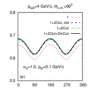
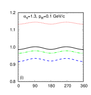
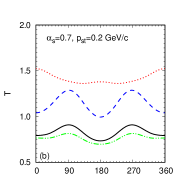
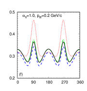
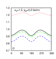
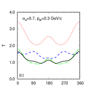
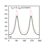
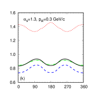
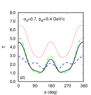
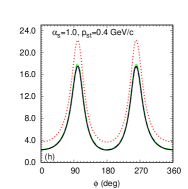
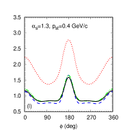
Figure 3: The azimuthal angle dependence of the transparency $T$ for $pd\to ppn$ at $p_{\rm lab}=4$ GeV/c and $\Theta_{\rm c.m.}=90\degree$. Different panels correspond to different values of $\alpha_{s}$ and $p_{st}$ as indicated. Dotted (red) lines – calculation with single rescattering amplitudes only. Dashed (blue) lines – calculation with single and double rescattering amplitudes where the latter include only the rescattering of outgoing protons and calculated according to Ref. Larionov (2023). Dash-double-dotted (green) lines – same as previous but with double rescattering amplitudes of the present work. Solid (black) lines – same as previous but with the double rescattering amplitudes of the incoming and outgoing protons.

The choice of large enough c.m. scattering angle is needed for keeping the $pp$ elastic scattering in a ’hard region’ ($|t|>1~{}\mbox{GeV}^{2}$). This is important for CT studies. However, according to the quark counting rule Matveev et al. (1973); Brodsky and Farrar (1973) the differential elastic $pp$ cross section $d\sigma_{pp}/dt$ at fixed $\Theta_{\rm c.m.}$ drops with increasing collision energy as $s^{-10}$. Thus, the cross section at $t=(4m^{2}-s)/2$, i.e. at $\Theta_{\rm c.m.}=90\degree$, becomes extremely small and difficult to study experimentally. Selecting smaller $|t|$ would strongly increase the cross section. For example, at $t=0.4(4m^{2}-s)/2$, that corresponds to $\Theta_{\rm c.m.}=53\degree$, the $pp$ differential cross section is two orders of magnitude larger than at $90\degree$ Frankfurt et al. (1995). Even at $p_{\rm lab}$ as small as 4 GeV/c the $pp$ scattering at $53\degree$ is still hard ($|t|=1.18~{}\mbox{GeV}^{2}$).

Fig. 4 shows the transparency at $p_{\rm lab}=4$ GeV/c and $\Theta_{\rm c.m.}=53\degree$. At $\alpha_{s}=1$ and 1.3, the azimuthal dependencies of $T$ at various spectator transverse momenta are quite similar to those at $\Theta_{\rm c.m.}=90\degree$. However, at $\alpha_{s}=0.7$, the $\phi$-dependence becomes substantially different from that at $\Theta_{\rm c.m.}=90\degree$. This is explained by the fact that the slowest outgoing proton has the transverse momentum component larger than the longitudinal one. The peak positions of the $\phi$-dependence of $T$ approximately correspond to the kinematics when the momentum of the slowest proton is orthogonal to the momentum of the spectator neutron which enhances the partial amplitudes with soft scattering of that proton.

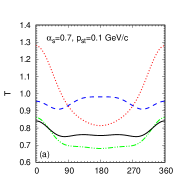
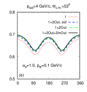
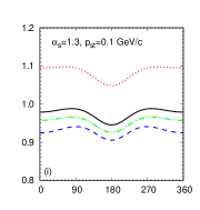
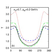
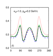
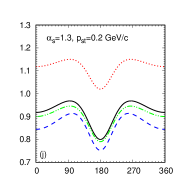
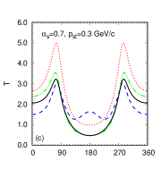
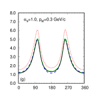
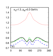
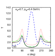
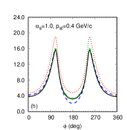
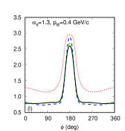
Figure 4: Same as Fig. 3, but for $\Theta_{\rm c.m.}=53\degree$.

It is expected that with increasing beam momentum the geometrical details of the double scattering amplitudes become less important. This is, indeed, visible from Figs. 5 and 6 which show the results at $p_{\rm lab}=15$ GeV/c for $\Theta_{\rm c.m.}=90\degree$ and $53\degree$, respectively. At $\alpha_{s}=1$ and 1.3, the difference between various treatments of the double scattering is not exceeding 10%. At $\alpha_{s}=0.7$ the difference is greater and, in addition, with an increase in the transverse momentum, the shape of the $\phi$-dependence of $T$ becomes different for the old and new treatment.

Interestingly, at $\Theta_{\rm c.m.}=53\degree$, $\alpha_{s}=1.3$, $p_{st}=0.4$ GeV/c, the sharp peak at $\phi=180\degree$ is visible for both $p_{\rm lab}=4$ and $15$ GeV/c. This feature persists whether double scattering is enabled or not, and is due to the orthogonality of the momenta of the spectator neutron and the slowest outgoing proton.

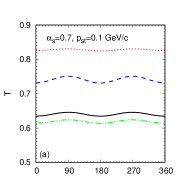
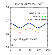
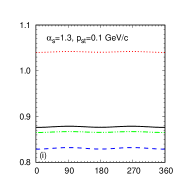
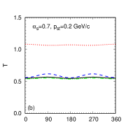
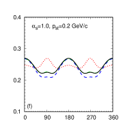
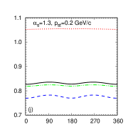
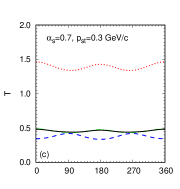
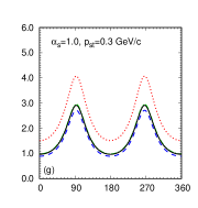
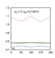
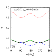
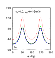
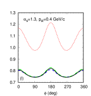
Figure 5: Same as Fig. 3, but for $p_{\rm lab}=15$ GeV/c.

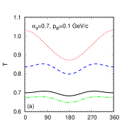
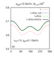
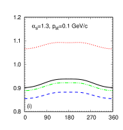
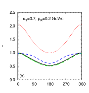
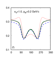
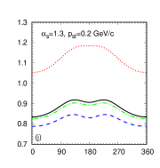
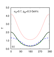
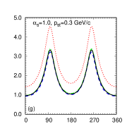
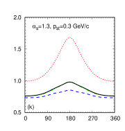
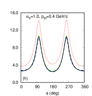
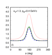
Figure 6: Same as Fig. 3, but for $p_{\rm lab}=15$ GeV/c and $\Theta_{\rm c.m.}=53\degree$.

4 Summary

Within the GEA framework, ladder diagrams with all possible soft elastic rescatterings were calculated for the process $d(p,pp)n$ at large $pp$ c.m. angles for proton beam momenta from several GeV/c to several tens of GeV/c. The main purpose was to accurately account for the deviations of the trajectories of the outgoing fast protons from the incoming beam direction. Accordingly, the propagators of the incoming and outgoing protons in the diagrams with soft rescattering were linearized with respect to the momentum transfers to the spectator nucleon along the asymptotic momenta of the protons. In the coordinate representation, this led to an ordering of the positions of the proton and neutron in the deuteron along the asymptotic momentum of the rescattered proton, which is expressed by the $\Theta$-function as a multiplicative factor. As a result, when at least one outgoing proton is produced at large angle in the deuteron rest frame, the amplitudes with double soft rescattering of the outgoing protons are corrected as compared to those of Refs. Frankfurt et al. (1997b); Larionov (2023). Moreover, the amplitudes with rescattering of both the incoming and outgoing protons become finite. The improved description has practically no effect in the transverse ($\alpha_{s}=1$) and backward ($\alpha_{s}>1$) spectator kinematics, however, becomes quite important in the forward ($\alpha_{s}<1$) one.

At the lowest beam momenta, $p_{\rm lab}\simeq 4-6$ GeV/c, where the search for CT effects is still possible, the effect of the improvement is comparable to the expected effect of CT on nuclear transparency. This range of momenta (per nucleon) is accessible at JINR nuclotron with deuteron beam and J-PARC, before the future FAIR, HIAF, and NICA facilities will come into operation and give an opportunity to study CT effects in a broader beam momentum range.

References

- Glauber (1959) R. J. Glauber, in Lectures in Theoretical Physics, Vol. 1, edited by W. E. Brittin and L. G. Dunham (Interscience Publishers, Inc., New York, 1959) p. 315.
- Glauber and Matthiae (1970) R. J. Glauber and G. Matthiae, Nucl. Phys. B21, 135 (1970).
- Gribov (1969) V. N. Gribov, Zh. Eksp. Teor. Fiz. 57, 1306 (1969).
- Bertocchi (1972) L. Bertocchi, Nuovo Cim. A 11, 45 (1972).
- Frankfurt et al. (1997a) L. L. Frankfurt, M. M. Sargsian, and M. I. Strikman, Phys. Rev. C 56, 1124 (1997a), arXiv:nucl-th/9603018 .
- Frankfurt et al. (1997b) L. L. Frankfurt, E. Piasetzky, M. M. Sargsian, and M. I. Strikman, Phys. Rev. C 56, 2752 (1997b), arXiv:hep-ph/9607395 .
- Sargsian (2001) M. M. Sargsian, Int. J. Mod. Phys. E 10, 405 (2001), arXiv:nucl-th/0110053 .
- Larionov et al. (2014) A. B. Larionov, M. Strikman, and M. Bleicher, Phys. Rev. C 89, 014621 (2014), arXiv:1312.2150 [nucl-th] .
- Boeglin and Sargsian (2024) W. U. Boeglin and M. M. Sargsian, Phys. Lett. B 854, 138742 (2024), arXiv:2402.13411 [nucl-th] .
- Larionov (2023) A. B. Larionov, Phys. Rev. C 107, 014605 (2023), arXiv:2208.08832 [nucl-th] .
- Larionov et al. (2019) A. B. Larionov, A. Gillitzer, and M. Strikman, Eur. Phys. J. A 55, 154 (2019), arXiv:1905.10419 [nucl-th] .
- Larionov and Strikman (2020) A. B. Larionov and M. Strikman, Eur. Phys. J. A 56, 21 (2020), arXiv:1909.00379 [nucl-th] .
- Larionov (2022) A. B. Larionov, MDPI Physics 4, 294 (2022).
- Larionov (2024) A. B. Larionov, (2024), arXiv:2409.07845 [nucl-th] .
- Larionov et al. (2018) A. B. Larionov, A. Gillitzer, J. Haidenbauer, and M. Strikman, Phys. Rev. C98, 054611 (2018), arXiv:1807.05105 [nucl-th] .
- Matveev et al. (1973) V. A. Matveev, R. M. Muradian, and A. N. Tavkhelidze, Lett. Nuovo Cim. 7, 719 (1973).
- Brodsky and Farrar (1973) S. J. Brodsky and G. R. Farrar, Phys. Rev. Lett. 31, 1153 (1973).
- Frankfurt et al. (1995) L. Frankfurt, E. Piasetsky, M. Sargsian, and M. Strikman, Phys. Rev. C 51, 890 (1995), arXiv:nucl-th/9405003 .