Real-bogus scores for active anomaly detection

Abstract

In the task of anomaly detection in modern time-domain photometric surveys, the primary goal is to identify astrophysically interesting, rare, and unusual objects among a large volume of data. Unfortunately, artifacts — such as plane or satellite tracks, bad columns on CCDs, and ghosts — often constitute significant contaminants in results from anomaly detection analysis. In such contexts, the Active Anomaly Discovery (AAD) algorithm allows tailoring the output of anomaly detection pipelines according to what the expert judges to be scientifically interesting. We demonstrate how the introduction real-bogus scores, obtained from a machine learning classifier, improves the results from AAD. Using labeled data from the SNAD ZTF knowledge database, we train four real-bogus classifiers: XGBoost, CatBoost, Random Forest, and Extremely Randomized Trees. All the models perform real-bogus classification with similar effectiveness, achieving ROC-AUC scores ranging from 0.93 to 0.95. Consequently, we select the Random Forest model as the main model due to its simplicity and interpretability. The Random Forest classifier is applied to 67 million light curves from ZTF DR17. The output real-bogus score is used as an additional feature for two anomaly detection algorithms: static Isolation Forest and AAD. While results from Isolation Forest remained unchanged, the number of artifacts detected by the active approach decreases significantly with the inclusion of the real-bogus score, from 27 to 3 out of 100. We conclude that incorporating the real-bogus classifier result as an additional feature in the active anomaly detection pipeline significantly reduces the number of artifacts in the outputs, thereby increasing the incidence of astrophysically interesting objects presented to human experts.

[sai] organization=Lomonosov Moscow State University, Sternberg Astronomical Institute, addressline=Universitetsky pr. 13, city=Moscow, postcode=119234, country=Russia

[hse] organization=National Research University Higher School of Economics, addressline=21/4 Staraya Basmannaya Ulitsa, city=Moscow, postcode=105066, country=Russia

[clermont] organization=Université Clermont Auvergne, CNRS/IN2P3, LPCA, city=Clermont-Ferrand, postcode=63000, country=France

[ind] organization=Independent researcher,

[mcwilliams] organization=McWilliams Center for Cosmology and Astrophysics, Department of Physics, Carnegie Mellon University, city=Pittsburgh, postcode=PA 15213, country=USA

[urbana] organization=Department of Astronomy, University of Illinois at Urbana-Champaign, addressline=1002 West Green Street, city=Urbana, postcode=IL 61801, country=USA

[iki] organization=Space Research Institute of the Russian Academy of Sciences (IKI), addressline=84/32 Profsoyuznaya Street, city=Moscow, postcode=117997, country=Russia

[surrey] organization=Physics Department, University of Surrey, addressline=Stag Hill Campus, GU2 7XH, city=Guildford, country=UK

1 Introduction

Modern sky surveys offer the opportunity to automatically observe a vast number of astrophysical objects across different classes. For instance, the Zwicky Transient Facility (ZTF; Bellm et al. 2019) generates about 2 terabytes of data per night, and the upcoming Vera C. Rubin Observatory Legacy Survey of Space and Time (LSST; LSST Science Collaboration et al. 2009) is expected to increase this amount by an order of magnitude. When dealing with such large volumes of data, machine learning (ML) methods are unavoidable, especially in tasks such as classification and anomaly detection (e. g., Baron 2019; Ishida 2019; Chen et al. 2020; Malik et al. 2022; Pruzhinskaya et al. 2023). However, the task of anomaly detection is particularly challenging due to the inherent nature of searching for statistical deviations in the data, which often results in a significant number of outliers being artifacts of automatic image processing, such as defocusing, bad columns, bright star spikes, ghosts, etc. For example, in Malanchev et al. (2021), 68 percent of outliers found by anomaly detection algorithms in the third ZTF data release (DR) were identified as bogus light curves. Around 80 instances of data artifacts were discovered as unwanted contaminants during the search for gravitational self-lensing binaries with ZTF (Crossland et al., 2023). Similarly, Sánchez-Sáez et al. (2021) encountered an overwhelming amount of bogus among the 8809 anomalies selected while searching for Changing-state AGNs in the ZTF DR5.

Given limited human resources, it is crucial to avoid spending time on non-astrophysical candidates. Active anomaly detection algorithms partly address this issue by incorporating feedback from human experts, which helps fine-tuning the algorithm and reduces the number of astrophysically uninteresting objects (Ishida et al., 2021). However, artifacts, due to their diversity, can occupy different regions of the parameter space, and even active algorithms cannot guarantee their elimination from outliers after several iterations.

One way to approach this problem is to make a real-bogus classification and then reject all objects that the classifier considered as artifacts. For example, this was done for Nearby Supernova Factory (Aldering et al., 2002) by Bailey et al. (2007) and other time domain surveys such as The Palomar Transient Factory (PTF; Brink et al. 2013), the Dark Energy Survey (DES; Goldstein et al. 2015), the Panoramic Survey Telescope and Rapid Response System (Pan-STARRS; Wright et al. 2015). Nowadays, neural network approaches are actively used for this purpose. For example, Weston et al. (2024) used difference imaging and convolutional neural networks for real-bogus classification in the Asteroid Terrestrial-impact Last Alert System (ATLAS; Tonry et al. 2018). Acero-Cuellar et al. (2023) used data from DES and investigated the performance of convolutional neural networks without using template subtraction. Deep learning methods are also used on ZTF survey data in real-bogus classification tasks (e. g., Duev et al. 2019; Carrasco-Davis et al. 2021; Semenikhin 2024).

The SNAD team has been working on the development and adaptation of anomaly detection techniques for astronomical data since 2018. In this work, we present and integrate into the SNAD pipeline a novel approach designed to reduce even further the number of artifacts presented to the expert in sequential iterations of the adaptive learning cycle. The idea involves the development of a real-bogus classifier whose predictions are used as an additional feature for each data instance. These enhanced data are then fed into the Active Anomaly Discovery (AAD; Das et al. 2016; Ishida et al. 2021) algorithm. It has been demonstrated that with this approach, AAD learns significantly faster to avoid returning artifacts to the expert, thus saving the expert’s time.

The article is structured as follows: Section 2 describes the data used for training and testing. Section 3 is dedicated to the construction of real-bogus classifiers. Section 4 presents a comparison of the performance of anomaly detection methods with and without real-bogus scores. Finally, Sections 5 and 6 contain the discussion and conclusions, respectively.

2 Data

The classifier is developed to increase the efficiency of anomaly detection in the data from the Zwicky Transient Facility, an automated wide-field sky survey. ZTF is conducted at the Palomar Observatory in California, USA, using a 1.26-m Samuel Oschin telescope with a field of view of approximately $47$ square degrees. The survey operates in three photometric passbands ($zg$, $zr$, $zi$). Data from ZTF are provided in two formats: alerts and data releases. Alerts are issued in real-time, while data releases contain light curves of variable objects over the entire observation period. In this work, we use the $zr$-band light curves from the data releases only.

2.1 Real-bogus dataset

The anomaly knowledge base (AKB; see Section 4 in Malanchev et al. 2023) was created by experts from the SNAD team during the scrutiny of the outputs of anomaly detection algorithms run on various ZTF DRs. Each ZTF object, identified by the object ID (OID), is classified according to the SNAD classification scheme (see examples in Fig. 1) based on extensive analysis, including visual screening, literature review, photometric model fitting, and follow-up observations. As of July 2023, the database comprised 3311 objects: 1646 artifacts and 1665 astrophysical objects of different types. We use this dataset, referred to as the real-bogus dataset, to train and test real-bogus classifiers.

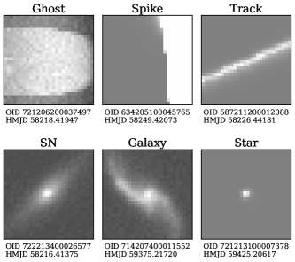
Figure 1: Object examples of different classes from ZTF data. Each image has size of 28 px $\times$ 28 px, $1~{}{\rm px}=1.012^{\prime\prime}$.

2.2 Target dataset

For the anomaly detection task we used light curves from ZTF DR17 within the MJD interval $\in\left[59184;59524\right]$ subjected to the following cuts: at least 100 observations and $\left|b\right|$ $>15^{\circ}$, where $b$ is the galactic latitude. This resulted in approximately 67 millions OIDs that make up the target dataset. We ran the Isolation Forest and the Active Anomaly Discovery algorithm on this dataset.

2.3 Light curve features

For each light curve we extracted 54 features using the lightcurve package described at Malanchev et al. (2021). Some of them have a simple form, such as flux amplitude or mean value. Others have a more complex dependency with the light curve shape, such as skewness or optimized parameters of the Bazin function from Bazin et al. (2009). We name this feature set initial.

3 Real-bogus classifiers

As classifiers, we consider 4 of the most popular models for working with tabular data. Two of them are based on gradient boosting (Friedman, 2001): XGBoost (Chen and Guestrin, 2016) and CatBoost (Dorogush et al., 2018). The others have simpler architectures and interpretability: Random Forest (Breiman, 2001) and Extremely Randomized Trees (ExtraTrees, Geurts et al. 2006). The models’ parameters were tuned using Optuna framework (see Table 1). When selecting parameters, the algorithm aimed to maximize accuracy. We choose this metric so it does not coincide with our main validation metric (Receiver Operating Characteristic – Area Under the Curve (ROC-AUC)).

XGBoost
booster	dart
lambda	0
alpha	0
subsample	0.79
colsample_bytree	0.66
max_depth	9
min_child_weight	3
eta	0.02
gamma	0
grow_policy	lossguide
sample_type	uniform
normalize_type	tree
rate_drop	0.1
skip_drop	0
CatBoost
objective	CrossEntropy
colsample_bylevel	0.07
depth	7
boosting_type	Plain
bootstrap_type	Bayesian
bagging_temperature	1.53
Random Forest
max_depth	18
n_estimators	830
Extremely Randomized Trees
max_depth	39
n_estimators	251
max_features†	1

Table 1: Parameters for real-bogus classifiers optimized with Optuna. ^†This parameter was not varied and set equal to 1.

We use objects and corresponding labels (0 stands for an artefact, 1 – astrophysical object) from the real-bogus dataset for training classifiers. The real-bogus classifier works in the following way: we feed light curve features to one of the classical machine learning method listed above, which returns a real-bogus score in the range $[0,1]$. The closer the number is to 0, the more confident the model is that the light curve represents an artefact.

Since the real-bogus dataset is relatively small (3311 objects), we use a k-fold ($k=5$) cross-validation when training the classifiers. In this method, we divide the available data into $k$ subsets. Then, a model is trained on union of $k-1$ subsets and evaluated on the remaining one, called the test set. This process is repeated $k$ times, each time using a different subset as the test set. As a result, $k$ model quality metric estimates are obtained, which are then averaged to compute the final estimate. This approach allows us to avoid overfitting and to obtain a more reliable efficiency estimate.

3.1 Validation of classifiers

In order to determine the predicted class of an object, it is necessary to choose a threshold for the real-bogus score. However, in this work, the prediction of the classifier serves as an additional source of information for the Active Anomaly Discovery algorithm (see Section 4). In this case, the determination of a specific threshold is the prerogative of the AAD algorithm based on expert feedback. Moreover, technically, such a threshold may vary for different regions of the feature space. Therefore, we chose ROC-AUC as a main quality metric for the real-bogus classifiers. As additional quality metrics, we also considered Accuracy and F1-score with the standard threshold set to 0.5 as well as ROC-curves (see Fig. 2).

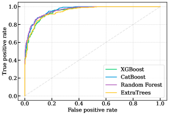
Figure 2: ROC-curve examples of trained real-bogus classifiers for one of the cross-validation splits.

From Table 2, which presents the final values of the quality metrics averaged over the test sets, and Fig. 2, it can be seen that the 4 considered models achieve similar performances. Therefore, we select the Random Forest as the main model because it is the simplest and most interpretable algorithm. All the real-bogus scores presented below were obtained using this model.

Model name	ROC-AUC	Accuracy	F1-score
Random Forest	0.94 $\pm$ 0.01	0.87 $\pm$ 0.02	0.87 $\pm$ 0.02
ExtraTrees	0.93 $\pm$ 0.01	0.85 $\pm$ 0.01	0.85 $\pm$ 0.01
XGBoost	0.93 $\pm$ 0.01	0.85 $\pm$ 0.02	0.85 $\pm$ 0.01
CatBoost	0.95 $\pm$ 0.01	0.87 $\pm$ 0.02	0.87 $\pm$ 0.02

Table 2: Real-bogus classifiers results. The metric values are averaged over 5 test sets, as well as the standard deviation.

3.2 Inference

Fig. 3 demonstrates the distributions of real-bogus score based on the Random Forest model. The histogram of predictions for objects from the real-bogus dataset, as expected, has a bimodal distribution, while the distribution for target dataset resembles a bell curve. From this, we conclude that our classifier, trained on objects identified by SNAD experts as outliers in ZTF DRs, is capable of classifying such outliers. However, when the classifier see features of an object with a distribution not represented in the real-bogus dataset, it outputs a real-bogus score close to 0.5. This can be interpreted as the model being unsure about the class to which this object belongs. This reduces the likelihood of the classifier labeling an interesting anomaly as an artefact.

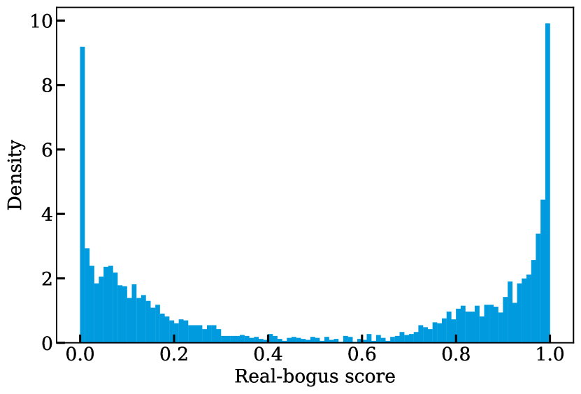
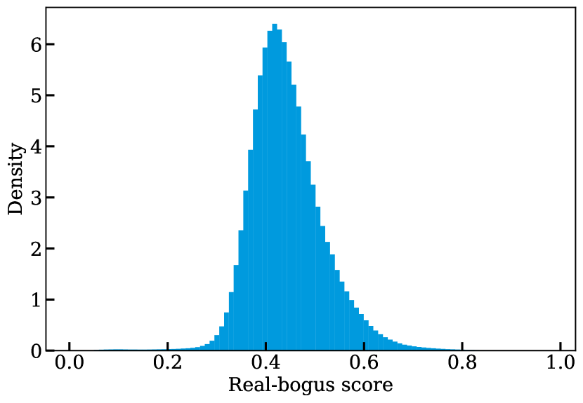
Figure 3: Histograms of real-bogus classifier (Random Forest model) predictions. Left: objects from real-bogus dataset (3311 objects). Right: objects from target dataset (approximately 67 millions objects).

4 Anomaly detection with real-bogus scores

In the SNAD pipeline, anomaly detection is carried out using algorithms based on random trees. The input data consist of light curve features, based on which the algorithm ranks objects according to their anomaly score. Then, a reasonable sample of the most anomalous objects is provided to the expert for manual verification. The sample size (budget) is a hyperparameter, which is defined by expert.

Integration of the real-bogus score into the anomaly detection algorithm is achieved by adding the classifier’s prediction to the initial set of features (described in Section 2.3). We refer to the resulting set matrix as the augmented feature set, i.e., with real-bogus score. Next, we feed this matrix to the anomaly detection algorithm.

Below we test two anomaly detection algorithms and feature sets: Isolation Forest and Active Anomaly Detection, are applied on the initial feature set and on the augmented. Our goal is to understand how the addition of a new feature affects the efficiency of anomaly detection.

4.1 Isolation forest

Isolation Forest (IF; Liu et al. 2008) is an ensemble of random trees that allows for identifying anomalies within the data. The main assumption of this algorithm is that anomalies are isolated in the feature space from normal objects. The fewer random splits a tree needs to separate an object from the rest, the more anomalous it is considered. The anomaly score of the IF is inversely proportional to the average number of such splits across all trees in the ensemble.

In this work, we use an IF with 100 trees, each using 256 objects for construction.

We independently run the IF from the coniferest Python library on both feature sets. Fig. 4 shows histograms of classifier prediction distributions for objects with the highest anomaly scores (for the first hundred most anomalous objects and for 5000). The blue histogram represents the result for the IF run on the initial feature set, while the red one shows outcomes from the augmented set. It can be seen that the histograms of the 100 most anomalous objects in both cases have a similar shape, with a prevalence of objects with high real-bogus scores. However, the distributions for 5000 objects show significant differences: for the initial feature set, there are significantly more objects with low real-bogus scores, and conversely, for the augmented set, there are significantly more objects with high real-bogus scores. As a result, it can be concluded that the real-bogus classifier’s predictions help decision trees in the IF to group artefacts together, so they become less anomalous. However, this effect is noticeable when considering 5000 anomaly candidates, making this method inefficient for practical applications.

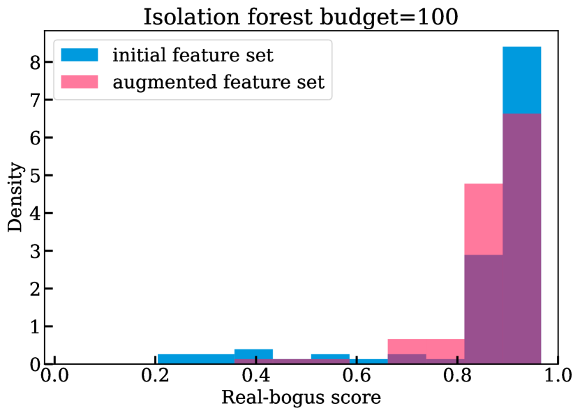
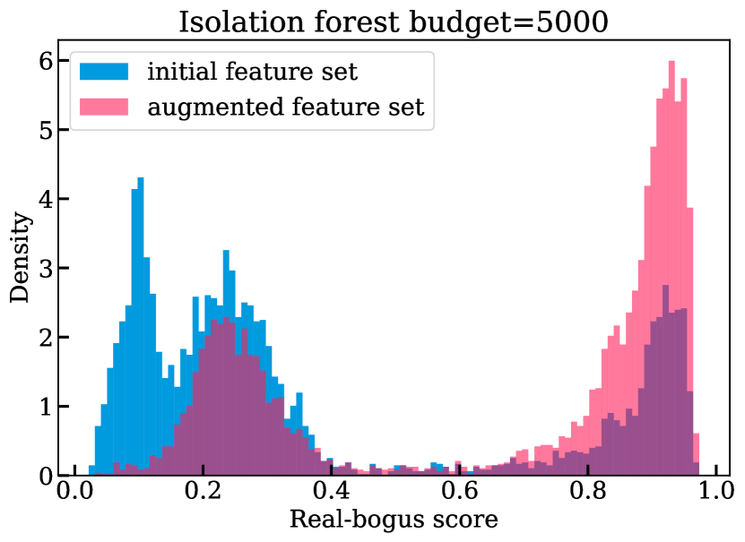
Figure 4: Distributions of real-bogus classifier (Random Forest model) predictions for two feature sets. Left: histogram for 100 objects with highest anomaly scores. Right: histogram for 5000 objects with highest anomaly scores.

We manually verified 100 objects with the highest anomaly scores for both sets of features. The result is the same – in both cases, out of 100 objects, 13 are artefacts.

4.2 Active Anomaly Discovery

Active Anomaly Discovery (Das et al., 2016, 2017) is an algorithm based on the IF that adapts to expert actions on the fly. During the model initialization stage, an IF is trained. Then, the object with the highest anomaly score is sent for review to an expert who provides feedback on its classification (anomalous or nominal). The obtained feedback is used to update the base model by changing its parameters. Subsequently, the original data is fed into the modified IF. These steps are repeated until a certain number of reviewed objects (budget) is reached. This algorithm is flexible to changes in the expert requirements, as the user chooses what to consider as an anomaly and what to consider as a normal object (see example usage in Ishida et al. 2021; Pruzhinskaya et al. 2023).

As with IF, AAD was independently applied to the data represented by the initial feature set and the augmented. During the operation, the expert classified artefacts with the label “NO” (0), which corresponds to nominal samples, and with the label “YES” (1) – to indicate real astrophysical events. For both feature sets, 100 objects were checked. The ratio of artefacts to the total number of scrutinized objects is $27/100$ for the initial feature set, and $3/100$ for the augmented feature set.

The dependency of the fraction of anomalies on the number of candidates verified by the expert is presented in Fig. 5. It can be seen that AAD, receiving input data represented by the initial feature set (blue line), returns significantly more artefacts for expert verification compared to AAD trained on data with real-bogus score (red line). Therefore, it can be concluded that the augmented feature set accelerates the training of the AAD model compared to the initial set.

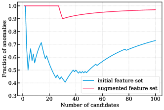
Figure 5: Results of running AAD on two feature sets: the dependence of the anomalies fraction on the number of verified candidates.

5 Discussion on the forest structure

To analyze the change in the structure of the IF when adding a new feature, we constructed IF leaf vectors $z$ (Das et al., 2017). For instance $x$ there is a vector $z\in\{0,1\}^{N}$, where $N$ is the number of leaves in the IF ensemble. Each component of $z$ stands for particular leaf in IF, $z_{i}=1$ means that instance $x$ fell into i-th leaf, while $z_{i}=0$ means the opposite. By construction $\sum_{i=1}^{N}{z_{i}}$ equals to number of trees in the IF.

We computed $z$ for each object from the real-bogus dataset represented by the initial and augmented feature sets. Then the confusion matrix can be estimated for every $z_{i}$ as if it was a real-bogus classifier prediction:

$$\mathrm{CM}_{i}=\begin{bmatrix}\mathrm{TN}_{i}&\mathrm{FP}_{i}\\ \mathrm{FN}_{i}&\mathrm{TP}_{i}\end{bmatrix},$$ (1)

where $\mathrm{TN}_{i}$ is the number of real objects with $z_{i}=0$, $\mathrm{FP}_{i}$ is the number of real objects with $z_{i}=1$, $\mathrm{FN}_{i}$ is the number of artifact objects with $z_{i}=0$, $\mathrm{TP}_{i}$ is the number of artifact objects with $z_{i}=1$. We use accuracy score:

$$\mathrm{Accuracy~{}score}_{i}=\frac{\mathrm{TN}_{i}+\mathrm{TP}_{i}}{M},$$ (2)

(where $M$ – number of objects in the real-bogus dataset) to explore artifact sensibility of every single leaf. Essentially, this means that the higher the value of the accuracy score for a leaf, the more often artefacts are encountered in that leaf and the less frequently astrophysical objects are found there. For the majority of leafs, the score is expected be $0.5$. Fig. 6 shows the accuracy scores for each leaf in the IF. According to this figure, it can be observed that with additional information from the real-bogus classifier, the IF occasionally creates leaves where artefacts are encountered much more frequently (Average score $>0.8$). Conversely, the IF without classifier predictions does not have such leaves as it was expected.

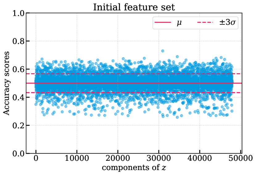
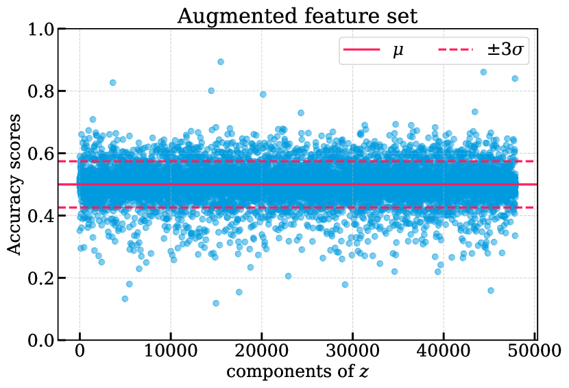
Figure 6: Accuracy score for each leaf in IF. Left: Leafs from IF trained on initial feature set. Right: Leafs from IF trained on augmented feature set. Both IFs have 1000 trees. Although for the majority of leafs accuracy score stay the same when adding new feature, a few of them become significantly better discriminator – larger number of extreme behavior in the right hand plot.

As discussed in Section 4.1, there is no difference between two feature sets when running IF with budget $=100$. This is due to the fact that IF calculates anomaly score as average random splits needed to separate an object from the rest (across the number of trees in the ensemble), so several leaves cannot significantly alter the result.

However, the presence of such leaves in the AAD structure significantly affects the final result. This is because the anomaly score in AAD is not calculated as the average number of splits needed to isolate an object, but as a weighted sum where the weights are the optimized parameters of the leaves. Therefore, AAD can effectively incorporate additional information from the classifier, which is confirmed in practice (see Fig. 5).

6 Conclusions

In this work, we focus on reducing the fraction of artefacts presented to the expert by the AAD algorithm. We started from the SNAD knowledge database, which consists of 3311 objects represented by light curve features (Malanchev et al., 2023) and whose labels were assigned by experts after visual inspection. This data set was used as a training set for 4 different real-bogus classifiers. Comparing their performance metrics, we selected the Random Forest model, for which the ROC-AUC $=0.94\pm 0.01$. The classification scores obtained from this classifier were then used as an additional feature in the data input to two anomaly detection methods: static Isolation Forest and Active Anomaly Discovery. We found that additional information from the real-bogus classifier allows IF to identify feature subspaces where artefacts group together. However, the desired reduction in the fraction of artefacts is only observed with large budgets. Considering only the 100 objects with highest anomaly score, the artifact ratios are the same for both feature sets (with and without the real-bogus classification scores). Meanwhile, the rate to which AAD presents real objects to the expert is significantly accelerated by using a feature set containing the real-bogus score. The effectiveness of this approach has been demonstrated in practice: $27/100$ artefact ratio for initial feature set against $3/100$ for augmented feature set.

The approach proposed in this work can be applied to other classes of objects (e. g., supernovae vs. non-supernovae). We can train several binary classifiers targeting different classes and then add the resulting predictions as new features to the input data. The results shown in this work indicate that one can expect significant speed up the rate to which AAD adapts to the feedback from the user.

The relevance of this work is highlighted by the forthcoming projects like LSST, which will generate an order of magnitude more data than ZTF. Filtering artefacts in such a data stream will become critically important.

References

- Acero-Cuellar et al. (2023) Acero-Cuellar, T., Bianco, F., Dobler, G., Sako, M., Qu, H., Collaboration, T.L.D.E.S., 2023. What’s the difference? the potential for convolutional neural networks for transient detection without template subtraction. The Astronomical Journal 166, 115. URL: https://dx.doi.org/10.3847/1538-3881/ace9d8, doi:10.3847/1538-3881/ace9d8.
- Aldering et al. (2002) Aldering, G., Adam, G., Antilogus, P., Astier, P., Bacon, R., Bongard, S., Bonnaud, C., Copin, Y., Hardin, D., Henault, F., Howell, D.A., Lemonnier, J.P., Levy, J.M., Loken, S.C., Nugent, P.E., Pain, R., Pecontal, A., Pecontal, E., Perlmutter, S., Quimby, R.M., Schahmaneche, K., Smadja, G., Wood-Vasey, W.M., 2002. Overview of the Nearby Supernova Factory, in: Tyson, J.A., Wolff, S. (Eds.), Survey and Other Telescope Technologies and Discoveries, pp. 61–72. doi:10.1117/12.458107.
- Bailey et al. (2007) Bailey, S., Aragon, C., Romano, R., Thomas, R.C., Weaver, B.A., Wong, D., 2007. How to Find More Supernovae with Less Work: Object Classification Techniques for Difference Imaging. ApJ 665, 1246–1253. doi:10.1086/519832, arXiv:0705.0493.
- Baron (2019) Baron, D., 2019. Machine Learning in Astronomy: a practical overview. doi:10.48550/arXiv.1904.07248, arXiv:1904.07248.
- Bazin et al. (2009) Bazin, G., Palanque-Delabrouille, N., Rich, J., Ruhlmann-Kleider, V., Aubourg, E., Le Guillou, L., Astier, P., Balland, C., Basa, S., Carlberg, R.G., Conley, A., Fouchez, D., Guy, J., Hardin, D., Hook, I.M., Howell, D.A., Pain, R., Perrett, K., Pritchet, C.J., Regnault, N., Sullivan, M., Antilogus, P., Arsenijevic, V., Baumont, S., Fabbro, S., Le Du, J., Lidman, C., Mouchet, M., Mourão, A., Walker, E.S., 2009. The core-collapse rate from the Supernova Legacy Survey. A&A 499, 653–660. doi:10.1051/0004-6361/200911847, arXiv:0904.1066.
- Bellm et al. (2019) Bellm, E.C., Kulkarni, S.R., Graham, M.J., Dekany, R., Smith, R.M., Riddle, R., Masci, F.J., Helou, G., Prince, T.A., Adams, S.M., Barbarino, C., Barlow, T., Bauer, J., Beck, R., Belicki, J., Biswas, R., Blagorodnova, N., Bodewits, D., Bolin, B., Brinnel, V., Brooke, T., Bue, B., Bulla, M., Burruss, R., Cenko, S.B., Chang, C.K., Connolly, A., Coughlin, M., Cromer, J., Cunningham, V., De, K., Delacroix, A., Desai, V., Duev, D.A., Eadie, G., Farnham, T.L., Feeney, M., Feindt, U., Flynn, D., Franckowiak, A., Frederick, S., Fremling, C., Gal-Yam, A., Gezari, S., Giomi, M., Goldstein, D.A., Golkhou, V.Z., Goobar, A., Groom, S., Hacopians, E., Hale, D., Henning, J., Ho, A.Y.Q., Hover, D., Howell, J., Hung, T., Huppenkothen, D., Imel, D., Ip, W.H., Ivezić, Ž., Jackson, E., Jones, L., Juric, M., Kasliwal, M.M., Kaspi, S., Kaye, S., Kelley, M.S.P., Kowalski, M., Kramer, E., Kupfer, T., Landry, W., Laher, R.R., Lee, C.D., Lin, H.W., Lin, Z.Y., Lunnan, R., Giomi, M., Mahabal, A., Mao, P., Miller, A.A., Monkewitz, S., Murphy, P., Ngeow, C.C., Nordin, J., Nugent, P., Ofek, E., Patterson, M.T., Penprase, B., Porter, M., Rauch, L., Rebbapragada, U., Reiley, D., Rigault, M., Rodriguez, H., van Roestel, J., Rusholme, B., van Santen, J., Schulze, S., Shupe, D.L., Singer, L.P., Soumagnac, M.T., Stein, R., Surace, J., Sollerman, J., Szkody, P., Taddia, F., Terek, S., Van Sistine, A., van Velzen, S., Vestrand, W.T., Walters, R., Ward, C., Ye, Q.Z., Yu, P.C., Yan, L., Zolkower, J., 2019. The Zwicky Transient Facility: System Overview, Performance, and First Results. PASP 131, 018002. doi:10.1088/1538-3873/aaecbe, arXiv:1902.01932.
- Breiman (2001) Breiman, L., 2001. Random forests. Machine Learning 45, 5–32. URL: https://doi.org/10.1023/A:1010933404324, doi:10.1023/A:1010933404324.
- Brink et al. (2013) Brink, H., Richards, J.W., Poznanski, D., Bloom, J.S., Rice, J., Negahban, S., Wainwright, M., 2013. Using machine learning for discovery in synoptic survey imaging data. MNRAS 435, 1047–1060. doi:10.1093/mnras/stt1306, arXiv:1209.3775.
- Carrasco-Davis et al. (2021) Carrasco-Davis, R., Reyes, E., Valenzuela, C., Förster, F., Estévez, P.A., Pignata, G., Bauer, F.E., Reyes, I., Sánchez-Sáez, P., Cabrera-Vives, G., Eyheramendy, S., Catelan, M., Arredondo, J., Castillo-Navarrete, E., Rodríguez-Mancini, D., Ruz-Mieres, D., Moya, A., Sabatini-Gacitúa, L., Sepúlveda-Cobo, C., Mahabal, A.A., Silva-Farfán, J., Camacho-Iñiguez, E., Galbany, L., 2021. Alert Classification for the ALeRCE Broker System: The Real-time Stamp Classifier. AJ 162, 231. doi:10.3847/1538-3881/ac0ef1, arXiv:2008.03309.
- Chen and Guestrin (2016) Chen, T., Guestrin, C., 2016. Xgboost: A scalable tree boosting system, in: Proceedings of the 22nd ACM SIGKDD International Conference on Knowledge Discovery and Data Mining, ACM. pp. 785–794. URL: http://dx.doi.org/10.1145/2939672.2939785, doi:10.1145/2939672.2939785.
- Chen et al. (2020) Chen, X., Wang, S., Deng, L., de Grijs, R., Yang, M., Tian, H., 2020. The Zwicky Transient Facility Catalog of Periodic Variable Stars. ApJS 249, 18. doi:10.3847/1538-4365/ab9cae, arXiv:2005.08662.
- Crossland et al. (2023) Crossland, A., Bellm, E.C., Klein, C., Davenport, J.R.A., Kupfer, T., Groom, S.L., Laher, R.R., Riddle, R., 2023. A Pilot Search for Gravitational Self-Lensing Binaries with the Zwicky Transient Facility. doi:10.48550/arXiv.2311.17862, arXiv:2311.17862.
- Das et al. (2016) Das, S., Wong, W.K., Dietterich, T.G., Fern, A., Emmott, A., 2016. Incorporating expert feedback into active anomaly discovery, in: Proceedings of the IEEE International Conference on Data Mining, pp. 853–858.
- Das et al. (2017) Das, S., Wong, W.K., Fern, A., Dietterich, T.G., Siddiqui, M.A., 2017. Incorporating feedback into tree-based anomaly detection. arXiv:1708.09441.
- Dorogush et al. (2018) Dorogush, A.V., Ershov, V., Gulin, A., 2018. Catboost: gradient boosting with categorical features support. arXiv:1810.11363.
- Duev et al. (2019) Duev, D.A., Mahabal, A., Masci, F.J., Graham, M.J., Rusholme, B., Walters, R., Karmarkar, I., Frederick, S., Kasliwal, M.M., Rebbapragada, U., Ward, C., 2019. Real-bogus classification for the Zwicky Transient Facility using deep learning. MNRAS 489, 3582–3590. doi:10.1093/mnras/stz2357, arXiv:1907.11259.
- Friedman (2001) Friedman, J.H., 2001. Greedy function approximation: a gradient boosting machine. Annals of statistics , 1189–1232.
- Geurts et al. (2006) Geurts, P., Ernst, D., Wehenkel, L., 2006. Extremely randomized trees. Machine Learning 63, 3–42. doi:10.1007/s10994-006-6226-1.
- Goldstein et al. (2015) Goldstein, D.A., D’Andrea, C.B., Fischer, J.A., Foley, R.J., Gupta, R.R., Kessler, R., Kim, A.G., Nichol, R.C., Nugent, P.E., Papadopoulos, A., Sako, M., Smith, M., Sullivan, M., Thomas, R.C., Wester, W., Wolf, R.C., Abdalla, F.B., Banerji, M., Benoit-Lévy, A., Bertin, E., Brooks, D., Carnero Rosell, A., Castander, F.J., da Costa, L.N., Covarrubias, R., DePoy, D.L., Desai, S., Diehl, H.T., Doel, P., Eifler, T.F., Fausti Neto, A., Finley, D.A., Flaugher, B., Fosalba, P., Frieman, J., Gerdes, D., Gruen, D., Gruendl, R.A., James, D., Kuehn, K., Kuropatkin, N., Lahav, O., Li, T.S., Maia, M.A.G., Makler, M., March, M., Marshall, J.L., Martini, P., Merritt, K.W., Miquel, R., Nord, B., Ogando, R., Plazas, A.A., Romer, A.K., Roodman, A., Sanchez, E., Scarpine, V., Schubnell, M., Sevilla-Noarbe, I., Smith, R.C., Soares-Santos, M., Sobreira, F., Suchyta, E., Swanson, M.E.C., Tarle, G., Thaler, J., Walker, A.R., 2015. Automated Transient Identification in the Dark Energy Survey. AJ 150, 82. doi:10.1088/0004-6256/150/3/82, arXiv:1504.02936.
- Ishida (2019) Ishida, E.E.O., 2019. Machine learning and the future of supernova cosmology. Nature Astronomy 3, 680–682. doi:10.1038/s41550-019-0860-6, arXiv:1908.02315.
- Ishida et al. (2021) Ishida, E.E.O., Kornilov, M.V., Malanchev, K.L., Pruzhinskaya, M.V., Volnova, A.A., Korolev, V.S., Mondon, F., Sreejith, S., Malancheva, A.A., Das, S., 2021. Active anomaly detection for time-domain discoveries. A&A 650, A195. doi:10.1051/0004-6361/202037709, arXiv:1909.13260.
- Liu et al. (2008) Liu, F.T., Ting, K.M., Zhou, Z.H., 2008. Isolation forest, in: 2008 Eighth IEEE International Conference on Data Mining, pp. 413–422. doi:10.1109/ICDM.2008.17.
- LSST Science Collaboration et al. (2009) LSST Science Collaboration, Abell, P.A., Allison, J., Anderson, S.F., Andrew, J.R., Angel, J.R.P., Armus, L., Arnett, D., Asztalos, S.J., Axelrod, T.S., Bailey, S., Ballantyne, D.R., Bankert, J.R., Barkhouse, W.A., Barr, J.D., Barrientos, L.F., Barth, A.J., Bartlett, J.G., Becker, A.C., Becla, J., Beers, T.C., Bernstein, J.P., Biswas, R., Blanton, M.R., Bloom, J.S., Bochanski, J.J., Boeshaar, P., Borne, K.D., Bradac, M., Brandt, W.N., Bridge, C.R., Brown, M.E., Brunner, R.J., Bullock, J.S., Burgasser, A.J., Burge, J.H., Burke, D.L., Cargile, P.A., Chandrasekharan, S., Chartas, G., Chesley, S.R., Chu, Y.H., Cinabro, D., Claire, M.W., Claver, C.F., Clowe, D., Connolly, A.J., Cook, K.H., Cooke, J., Cooray, A., Covey, K.R., Culliton, C.S., de Jong, R., de Vries, W.H., Debattista, V.P., Delgado, F., Dell’Antonio, I.P., Dhital, S., Di Stefano, R., Dickinson, M., Dilday, B., Djorgovski, S.G., Dobler, G., Donalek, C., Dubois-Felsmann, G., Durech, J., Eliasdottir, A., Eracleous, M., Eyer, L., Falco, E.E., Fan, X., Fassnacht, C.D., Ferguson, H.C., Fernandez, Y.R., Fields, B.D., Finkbeiner, D., Figueroa, E.E., Fox, D.B., Francke, H., Frank, J.S., Frieman, J., Fromenteau, S., Furqan, M., Galaz, G., Gal-Yam, A., Garnavich, P., Gawiser, E., Geary, J., Gee, P., Gibson, R.R., Gilmore, K., Grace, E.A., Green, R.F., Gressler, W.J., Grillmair, C.J., Habib, S., Haggerty, J.S., Hamuy, M., Harris, A.W., Hawley, S.L., Heavens, A.F., Hebb, L., Henry, T.J., Hileman, E., Hilton, E.J., Hoadley, K., Holberg, J.B., Holman, M.J., Howell, S.B., Infante, L., Ivezic, Z., Jacoby, S.H., Jain, B., R, Jedicke, Jee, M.J., Garrett Jernigan, J., Jha, S.W., Johnston, K.V., Jones, R.L., Juric, M., Kaasalainen, M., Styliani, Kafka, Kahn, S.M., Kaib, N.A., Kalirai, J., Kantor, J., Kasliwal, M.M., Keeton, C.R., Kessler, R., Knezevic, Z., Kowalski, A., Krabbendam, V.L., Krughoff, K.S., Kulkarni, S., Kuhlman, S., Lacy, M., Lepine, S., Liang, M., Lien, A., Lira, P., Long, K.S., Lorenz, S., Lotz, J.M., Lupton, R.H., Lutz, J., Macri, L.M., Mahabal, A.A., Mandelbaum, R., Marshall, P., May, M., McGehee, P.M., Meadows, B.T., Meert, A., Milani, A., Miller, C.J., Miller, M., Mills, D., Minniti, D., Monet, D., Mukadam, A.S., Nakar, E., Neill, D.R., Newman, J.A., Nikolaev, S., Nordby, M., O’Connor, P., Oguri, M., Oliver, J., Olivier, S.S., Olsen, J.K., Olsen, K., Olszewski, E.W., Oluseyi, H., Padilla, N.D., Parker, A., Pepper, J., Peterson, J.R., Petry, C., Pinto, P.A., Pizagno, J.L., Popescu, B., Prsa, A., Radcka, V., Raddick, M.J., Rasmussen, A., Rau, A., Rho, J., Rhoads, J.E., Richards, G.T., Ridgway, S.T., Robertson, B.E., Roskar, R., Saha, A., Sarajedini, A., Scannapieco, E., Schalk, T., Schindler, R., Schmidt, S., Schmidt, S., Schneider, D.P., Schumacher, G., Scranton, R., Sebag, J., Seppala, L.G., Shemmer, O., Simon, J.D., Sivertz, M., Smith, H.A., Allyn Smith, J., Smith, N., Spitz, A.H., Stanford, A., Stassun, K.G., Strader, J., Strauss, M.A., Stubbs, C.W., Sweeney, D.W., Szalay, A., Szkody, P., Takada, M., Thorman, P., Trilling, D.E., Trimble, V., Tyson, A., Van Berg, R., Vanden Berk, D., VanderPlas, J., Verde, L., Vrsnak, B., Walkowicz, L.M., Wandelt, B.D., Wang, S., Wang, Y., Warner, M., Wechsler, R.H., West, A.A., Wiecha, O., Williams, B.F., Willman, B., Wittman, D., Wolff, S.C., Wood-Vasey, W.M., Wozniak, P., Young, P., Zentner, A., Zhan, H., 2009. LSST Science Book, Version 2.0. doi:10.48550/arXiv.0912.0201, arXiv:0912.0201.
- Malanchev et al. (2023) Malanchev, K., Kornilov, M.V., Pruzhinskaya, M.V., Ishida, E.E.O., Aleo, P.D., Korolev, V.S., Lavrukhina, A., Russeil, E., Sreejith, S., Volnova, A.A., Voloshina, A., Krone-Martins, A., 2023. The SNAD Viewer: Everything You Want to Know about Your Favorite ZTF Object. PASP 135, 024503. doi:10.1088/1538-3873/acb292, arXiv:2211.07605.
- Malanchev et al. (2021) Malanchev, K.L., Pruzhinskaya, M.V., Korolev, V.S., Aleo, P.D., Kornilov, M.V., Ishida, E.E.O., Krushinsky, V.V., Mondon, F., Sreejith, S., Volnova, A.A., Belinski, A.A., Dodin, A.V., Tatarnikov, A.M., Zheltoukhov, S.G., (The SNAD Team), 2021. Anomaly detection in the Zwicky Transient Facility DR3. MNRAS 502, 5147–5175. doi:10.1093/mnras/stab316, arXiv:2012.01419.
- Malik et al. (2022) Malik, A., Moster, B.P., Obermeier, C., 2022. Exoplanet detection using machine learning. MNRAS 513, 5505–5516. doi:10.1093/mnras/stab3692, arXiv:2011.14135.
- Pruzhinskaya et al. (2023) Pruzhinskaya, M.V., Ishida, E.E.O., Novinskaya, A.K., Russeil, E., Volnova, A.A., Malanchev, K.L., Kornilov, M.V., Aleo, P.D., Korolev, V.S., Krushinsky, V.V., Sreejith, S., Gangler, E., 2023. Supernova search with active learning in ZTF DR3. A&A 672, A111. doi:10.1051/0004-6361/202245172, arXiv:2208.09053.
- Sánchez-Sáez et al. (2021) Sánchez-Sáez, P., Lira, H., Martí, L., Sánchez-Pi, N., Arredondo, J., Bauer, F.E., Bayo, A., Cabrera-Vives, G., Donoso-Oliva, C., Estévez, P.A., Eyheramendy, S., Förster, F., Hernández-García, L., Arancibia, A.M.M., Pérez-Carrasco, M., Sepúlveda, M., Vergara, J.R., 2021. Searching for Changing-state AGNs in Massive Data Sets. I. Applying Deep Learning and Anomaly-detection Techniques to Find AGNs with Anomalous Variability Behaviors. AJ 162, 206. doi:10.3847/1538-3881/ac1426, arXiv:2106.07660.
- Semenikhin (2024) Semenikhin, T.A., 2024. Neural network architecture for artifacts detection in ZTF survey. Systems and Means of Informatics 34, 70–79. URL: http://dx.doi.org/10.14357/08696527240106, doi:10.14357/08696527240106.
- Tonry et al. (2018) Tonry, J.L., Denneau, L., Heinze, A.N., Stalder, B., Smith, K.W., Smartt, S.J., Stubbs, C.W., Weiland, H.J., Rest, A., 2018. ATLAS: A High-cadence All-sky Survey System. PASP 130, 064505. doi:10.1088/1538-3873/aabadf, arXiv:1802.00879.
- Weston et al. (2024) Weston, J.G., Smith, K.W., Smartt, S.J., Tonry, J.L., Stevance, H.F., 2024. Training a convolutional neural network for real–bogus classification in the ATLAS survey. RAS Techniques and Instruments 3, 385–399. doi:10.1093/rasti/rzae027.
- Wright et al. (2015) Wright, D.E., Smartt, S.J., Smith, K.W., Miller, P., Kotak, R., Rest, A., Burgett, W.S., Chambers, K.C., Flewelling, H., Hodapp, K.W., Huber, M., Jedicke, R., Kaiser, N., Metcalfe, N., Price, P.A., Tonry, J.L., Wainscoat, R.J., Waters, C., 2015. Machine learning for transient discovery in Pan-STARRS1 difference imaging. MNRAS 449, 451–466. doi:10.1093/mnras/stv292, arXiv:1501.05470.