Exploring Multifractal Critical Phases in Two-Dimensional Quasiperiodic Systems

Abstract

The multifractal critical phase (MCP) fundamentally differs from extended and localized phases, exhibiting delocalized distributions in both position and momentum spaces. The investigation on the MCP has largely focused on one-dimensional quasiperiodic systems. Here, we introduce a two-dimensional (2D) quasiperiodic model with a MCP. We present its phase diagram and investigate the characteristics of the 2D system’s MCP in terms of wave packet diffusion and transport based on this model. We further investigate the movement of the phase boundary induced by the introduction of next-nearest-neighbor hopping by calculating the fidelity susceptibility. Finally, we consider how to realize our studied model in superconducting circuits. Our work opens the door to exploring MCP in 2D systems.

I Introduction

The interference of multiply scattered waves caused by disorder leads to the exponential decay of the wave function. This phenomenon is referred to as Anderson localization (AL) Anderson1958 ; RMP1 ; RMP2 ; Kramer1993 and is widely present in disordered systems. Additionally, quasiperiodic potentials can also induce AL, and have received widespread attention in both theoretical Soukoulis1981 ; DasSarma1988 ; Biddle2009 ; XLi2017 ; HYao2019 ; Ganeshan2015 ; Wang1 ; XDeng2019 ; Ribeiro ; YaruLiu and experimental Roati2008 ; Bloch4 ; An2018 ; JiasT ; TXiao2021 ; Weld ; HengFan studies in recent years. Quasiperiodic systems exhibit physics distinct from randomly disordered systems. Generally, in low-dimensional disordered systems, even a small amount of disorder can cause AL. However, even in one-dimensional (1D) quasiperiodic systems, Anderson transitions only occur when the quasiperiodic potential reaches a certain strength. This leads to phenomena usually seen in three-dimensional disordered systems, such as mobility edges (MEs), appearing in 1D quasiperiodic systems Soukoulis1981 ; DasSarma1988 ; Biddle2009 ; XLi2017 ; HYao2019 ; Ganeshan2015 ; Wang1 ; XDeng2019 ; Ribeiro ; YaruLiu ; Roati2008 ; Bloch4 ; An2018 ; JiasT . The ME represents the critical energy that separates localized and extended states, describing the Anderson transition driven by changes in energy. The transition between localized and delocalized states can also occur across the entire spectrum RPModel1 ; RPModel2 , meaning there is no ME, with the possibility of a critical point or even a multifractal critical phase (MCP). It was further discovered that in 1D quasiperiodic systems, not only critical points exist, but MCP can also be present TXiao2021 ; Weld ; HengFan ; WangYC2021 ; Kohmoto1990 ; WangMBC ; Ribeiro2 .

MCP is a fundamental physical phase distinct from the extended phase and the localized phase. It exhibits various interesting features, such as special spectral statistics energy1 ; energy2 and multifractal distribution of wave-functions mul1 ; mul2 . From the perspective of wave packet dynamics (WPD), the WPD of extended phase and localized phase are ballistic and localized Hiramoto ; Geisel1997 , respectively. Critical phases, however, are more diverse. Critical phases induced by quasiperiodic potentials typically approach normal diffusion Hiramoto ; Geisel1997 , while critical phases in Fibonacci chains may also exhibit super-diffusion or sub-diffusion FibonacciRMP . From the perspective of transport, in the extended phase, the magnitude of conductance does not depend on the system size, while in the critical (localized) phase, conductance will decay in a power-law (exponential) form with increasing 1D system size transport1 ; transport2 ; transport3 ; Wang2022 . it is interesting to note that multifractal critical states can also enhance the superconducting transition temperature enhance1 ; enhance2 ; enhance3 ; enhance4 or the quantum metric metric1 .

Previous studies on MEs and MCPs in quasiperiodic systems mainly focused on one dimension. In recent years, 2D quasiperiodic systems have gradually attracted attention 2D1 ; 2D2 ; 2D3 ; 2D4 ; 2D5 ; WangZhang ; 2DME0 ; 2DME1 ; 2DME2 . For example, research on MEs has been extended to 2D quasiperiodic systems WangZhang ; 2DME0 ; 2DME1 ; 2DME2 . However, studies on MCPs induced by quasiperiodic potentials in 2D systems have yet to emerge noteadd , leaving many of the properties of these systems unclear, such as how to perform finite-size scaling analysis on the eigenfunctions to determine the phase transition points and the associated critical exponents, and how the WPD and transport behaviors of the 2D MCP differ from those in the extended, localized, and one-dimensional cases.

In this work, we study a 2D quasiperiodic model. When the next-nearest-neighbor (NNN) hopping strength of this model is set to zero, this model can be separated into two 1D models with exact critical phases. Thus, we can determine the phase diagram of this model in the special case where the NNN hopping strength is zero. Using this special case as a benchmark, we explore a finite-size analysis method and find that it can accurately determine the phase boundary locations, which are consistent with the phase boundaries obtained through decomposition. This demonstrates the feasibility of this finite-size analysis method in 2D quasi-periodic systems. We further investigate the WPD and transport behavior of critical phases in 2D systems, comparing them with the 1D case. Furthermore, when the NNN hopping strength is not zero, this model cannot be separated into two 1D models. Numerical evidence demonstrates that it still exhibits critical phases, and we analyze the influence of the NNN hopping on the phase boundaries. Finally, we provide experimental schemes to realize this model.

II Model

On a 2D square lattice, we investigate the Hamiltonian

$$\begin{split}H=&\sum_{ij}[h^{x}_{i,j}c_{i,j}^{\dagger}c_{i+1,j}+h^{y}_{i,j}c_{i,j}^{\dagger}c_{i,j+1}+h.c.+V_{i,j}c_{i,j}^{\dagger}c_{i,j}]\\ &+\lambda_{3}\sum_{ij}(c_{i+1,j+1}^{\dagger}c_{i,j}+c_{i-1,j+1}^{\dagger}c_{i,j}+h.c.),\end{split}$$ (1)

with

$$\begin{split}h^{x}_{i,j}=&\cos[2\pi\alpha_{1}(i+\frac{1}{2})+\delta_{1}]+\lambda_{1},\\ h^{y}_{i,j}=&\cos[2\pi\alpha_{2}(j+\frac{1}{2})+\delta_{2}]+\lambda_{1},\\ V_{i,j}=&\lambda_{2}[\cos(2\pi\alpha_{1}i+\delta_{1})+\cos(2\pi\alpha_{2}j+\delta_{2})],\end{split}$$ (2)

where $c_{i,j}^{\dagger}(c_{i,j})$ creates (annihilates) an electron at position $(i,j)$, $\alpha_{1}$ and $\alpha_{2}$ are irrational numbers, $\delta_{1}$ and $\delta_{2}$ are arbitrary phase shift, $\lambda_{1}$ adjusts the nearest-neighbor hopping strength, $\lambda_{2}$ is the strength of the on-site quasiperiodic potential, and $\lambda_{3}$ is the strength of the NNN hopping. For convenience, we fix $\alpha_{1}=\frac{\sqrt{5}-1}{2}$, $\alpha_{2}=\frac{\sqrt{2}}{2}$, $\delta_{1}=\delta_{2}=0$ and unless otherwise stated, set that the sizes in two directions are equal, i.e., $L_{x}=L_{y}=L$.

III Without NNN hopping

III.1 Phase diagram

We first discuss the phase diagram of this model when the NNN hopping strength is zero (i.e., $\lambda_{3}=0$). We aim to find the solutions of eigenfunction $H|\Psi\rangle=E|\Psi\rangle$ from separation of variables. The Hamiltonian $H$ with $\lambda_{3}=0$ can be further written as $H=H_{x}+H_{y}=\sum_{j}H_{x,j}+\sum_{i}H_{y,i}$, with $H_{x,j}=\sum_{i}h^{x}_{i,j}c_{i,j}^{\dagger}c_{i+1,j}+h.c.+\lambda_{2}\sum_{i}\cos(2\pi\alpha_{1}i+\delta_{1})c_{i,j}^{\dagger}c_{i,j}$ and $H_{y,i}=\sum_{j}h^{y}_{i,j}c_{i,j}^{\dagger}c_{i,j+1}+h.c.+\lambda_{2}\sum_{j}\cos(2\pi\alpha_{2}j+\delta_{2})c_{i,j}^{\dagger}c_{i,j}$. $H_{x,j}$ with fixed $j$ and $H_{y,i}$ with fixed $i$ are two 1D extended Aubry-André (EAA) models with quasiperiodic hopping and quasiperiodic on-site potentials. Hence, the 2D model (1) is decoupled into two 1D EAA models  Kohmoto1990 ; WangMBC ; Takada ; Liu . We set $H_{x}|\psi_{x}\rangle=E_{x}|\psi_{x}\rangle$ and $H_{y}|\phi_{y}\rangle=E_{y}|\phi_{y}\rangle$ with $E_{x}+E_{y}=E$. We see $[H_{x},H_{y}]=0$, then the wavefunction can be written as the tensor product $|\Psi\rangle=|\psi_{x}\rangle\otimes|\phi_{y}\rangle$. Therefore, $|\Psi\rangle$ and $|\psi_{x}\rangle\otimes|\phi_{y}\rangle$ have similar extended, localized, and critical properties. According to the phase diagram of the EAA model, we similarly obtain the phase diagram of Hamiltonian (1), as shown in Fig. 1(a), where the critical, localized, and extanded phases correspond to the region I, II and III, respectively. To show the phase diagram, we calculate the average fractal dimension, which for any arbitrary $m$-th eigenstate $|\Psi_{m}\rangle=\sum_{j}^{L^{2}}\psi_{m,j}c^{\dagger}_{j}|\varnothing\rangle$ is related to the mean inverse participation ratio (MIPR) by $D=-\frac{\ln MIPR}{\ln L}$, with $MIPR=\frac{1}{L^{2}}\sum_{m=1}^{L^{2}}\sum_{j=1}^{L^{2}}|\psi_{m,j}|^{4}$. It is known that in the thermodynamic limit $L\rightarrow\infty$, the fractal dimension $D=2$ in the extended phase, $D=0$ in the localized phase, and $0<D<2$ in the critical phase [Fig. 1(a)]. The three phase boundaries are $\lambda_{1}=1$, $\lambda_{2}=2$ and $\lambda_{2}=2\lambda_{1}$, respectively.

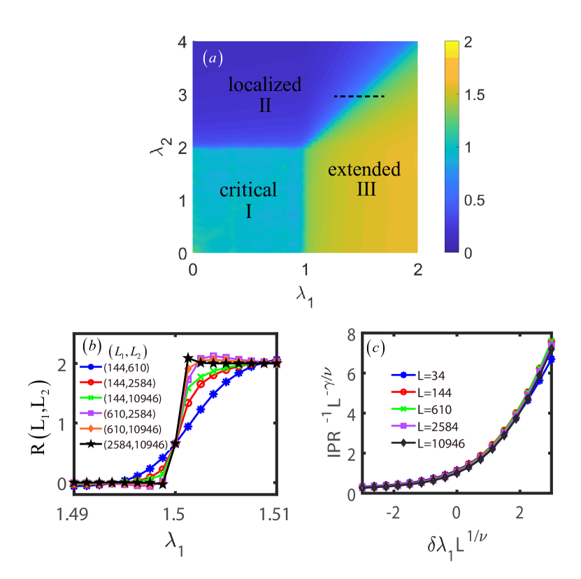
Figure 1: (a) Phase diagram of the 2D model (1) with $\lambda_{3}=0$ characterized by the fractal dimension. Here we take the system size $L=80$. The regions I, II and III correspond to the critical, localized, and extanded phases, respectively. (b)(c) The finite size scaling analysis near the localized-extended transition with $\lambda_{2}=3$ being fixed. (b) The plot of $R(L_{1},L_{2})$ as a function of $\lambda_{1}$ for several pairs of $(L_{1},L_{2})$. (c) The plot $IPR^{-1}L^{-\frac{\gamma}{\nu}}$ versus $\delta\lambda_{1}L^{\frac{1}{\nu}}$ for different sizes, all the curves convergence for $\nu=1$ and $\gamma=0.659\pm 0.004$.

Anderson transition is the continuous phase transition, where the scaling behavior occurs near the phase boundary, and critical exponent can be defined to characterize different types of universality classes. Near the critical point, we introduce the critical exponents $\nu$ and $\gamma$, which describe the divergence of the correlation and localization lengths $\xi$ and IPR close to the transition as

$$\xi\sim|\delta\lambda_{\alpha}|^{-\nu},\quad IPR\sim(\delta\lambda_{\alpha})^{\gamma},$$ (3)

where $\delta\lambda_{\alpha}=(\lambda_{\alpha}-\lambda_{\alpha,c})/\lambda_{\alpha,c}$ with $\alpha=1,2$, and $\lambda_{\alpha,c}$ being the phase transition point. This system can be analogized to the thermodynamic properties of the Ising model, with $M$ as the instantaneous magnetization of a system with $N$ spins. When the temperature exceeds the critical temperature, i.e., $T>T_{c}$, the thermal average of $M^{2}$ is written as $\langle M^{2}\rangle\propto\chi/N$, where $\chi$ is the magnetic susceptibility QPT1 ; QPT2 . We know that near the transition point, $M(T)\sim|T-T_{c}|^{\beta}$, $\chi\sim|T-T_{c}|^{-\gamma}$, and the correlation length $\xi\sim|T-T_{c}|^{-\nu}$ QPT1 ; QPT2 . We can correspond the latter two to the $IPR^{-1}$ and $\xi$ introduced earlier in Eq. (3), and $\langle M^{2}\rangle\propto\chi/N$ to

$$IPR^{-1}/L^{d}\sim(-\delta\lambda_{\alpha})^{2\beta}.$$ (4)

From Eq. (3) and Eq. (4), we can obtain $IPR\sim\xi^{-\gamma/\nu}$ and $IPR^{-1}/L^{d}\sim\xi^{-\beta/2\nu}$. At the transition point, where $\xi\sim L$, we have $IPR\sim L^{-\gamma/\nu}$ and $IPR^{-1}/L^{d}\sim L^{-\beta/2\nu}$. Then we can directly obtain the hyperscaling law $2\beta/\nu+\gamma/\nu=d$, which is also the same as the hyperscaling law at the phase transition point of the Ising model. By analogy with the scaling relationship for magnetization in a finite-size system, $M(L,T)\sim L^{-\beta/\nu}\times g_{M}((T-T_{c})L^{1/\nu})$, where $g_{M}$ is the scaling function, we assume the following finite size scaling relationship when the system is finite:

$$IPR^{-1}/L^{d}=L^{-2\beta/\nu}F(L^{\frac{1}{\nu}}\delta\lambda_{\alpha}),$$ (5)

where $F(x)$ is the scaling function. Using the hyperscaling law mentioned above, Eq. (5) simplifies to:

$$IPR^{-1}L^{-\frac{\gamma}{\nu}}=F(L^{\frac{1}{\nu}}\delta\lambda_{\alpha}),$$ (6)

The analogy between the scaling analysis near the phase transition point of the model we discussed and that of the Ising model is summarized in Table 1.

Ising model	The model we studied
$\xi\sim|T-T_{c}|^{-\nu}$	$\xi\sim|\delta\lambda_{\alpha}|^{-\nu}$
$\chi\sim|T-T_{c}|^{-\gamma}$	$IPR^{-1}\sim(\delta\lambda_{\alpha})^{-\gamma}$
$\langle M^{2}\rangle\propto\chi/N\sim|T-T_{c}|^{2\beta}$	$IPR^{-1}/L^{d}\sim(-\delta\lambda_{\alpha})^{2\beta}$
$M\sim L^{-\beta/\nu}g_{M}((T-T_{c})L^{1/\nu})$	$IPR^{-1}L^{-\frac{\gamma}{\nu}}=F(L^{\frac{1}{\nu}}\delta\lambda_{\alpha})$

Table 1: The analogy between the scaling analysis near the phase transition point of the Ising model and that of the model we discussed.

At the transition point, we have $\delta\lambda_{\alpha}=0$, and thus Eq. (6) becomes $IPR^{-1}=L^{\gamma/\nu}F(0)$. Then a function of two size-variables can be defined as FSZ1 ; FSZ2 :

$$R[L_{1},L_{2}]=\frac{\ln(IPR_{2}/IPR_{1})}{\ln(L_{1}/L_{2})},$$ (7)

which equals to $\gamma/\nu$ at the critical point for any pair $(L_{1},L_{2})$, where $L_{1}$ and $L_{2}$ represent two different system sizes. Fig. 1(b) displays the behaviors of $R[L_{1},L_{2}]$ as a function $\lambda_{1}$ for different pairs of $L_{1}$ and $L_{2}$ with fixed $\lambda_{2}=3$. From the crossing point, we can determine the critical point $\lambda_{1c}=1.500\pm 0.006$, which is consistent with phase boundary $\lambda_{2}=2\lambda_{1}$, and the corresponding critical exponent $\gamma/\nu\approx 0.66$. In Ref. WangZhang , we analytically obtained the localization length of a two-dimensional quasiperiodic vertex-decorated Lieb lattice and found the critical exponent $\nu=1$. Therefore, we directly choose $\nu=1$ here and plot $IPR^{-1}L^{-\frac{\gamma}{\nu}}$ as a function of $\delta\lambda_{1}L^{\frac{1}{\nu}}$ for different size in Fig. 1(c), we see all the curves superposed together, and the critical exponent $\gamma=0.659\pm 0.004$ errorbar , which is approximately twice the critical exponent of the Anderson transition induced by quasiperiodic potential in one dimension (According to the definition in Eq. (3), one can obtain the critical exponent $\gamma\approx 0.33$ near the Anderson transition point in a 1D quasiperiodic system HYao2019 ). Using the same approach, we can determine the transition points and critical exponents for the transition from critical phase to localized or extended phase.

III.2 Dynamics of Wave Packet and Transport Properties

We now discuss the diffusion dynamics of the wave packet, which can be measured directly from the experiments. Suppose a particle is initially localized at site $(p,q)$ and evolves according to the Hamiltonian. We study the mean square displacement

$$W(t)=\sqrt{\sum_{i,j}\bigg{[}(p-i)^{2}+(q-j)^{2}\bigg{]}\langle n_{i,j}(t)\rangle}$$ (8)

and the smoothed autocorrelation function

$$C(t)=\frac{1}{t}\int_{0}^{t}|\langle\Psi(0)|\Psi(t^{{}^{\prime}})\rangle|^{2}dt^{{}^{\prime}},$$ (9)

where $\langle n_{i,j}(t)\rangle$ is the time dependent particle numbers at site $(i,j)$ and $|\Psi(t)\rangle$ is the wavefunction at time $t$. Then the long time dynamical behavior of $W(t)$ and $C(t)$ are

$$W(t)\sim t^{\kappa},\quad C(t)\sim t^{-\beta},$$ (10)

where the $\kappa$ and $\beta$ depend on the energy spectrum and fractal characteristics of the wavefunctions Hiramoto ; ZhongJX ; Ketzmerick . Figs. 2(a) and (b) show the evolution of $W(t)$ and $C(t)$. The parameters of blue, red, and green lie in the extended, critical, and localized phases, respectively. The dynamical index $\kappa$ is similar to the 1D case: $\kappa=1$ signifies the ballistic evolution in the extended phase, $\kappa=0$ indicates localization in the localized phase, and $\kappa\approx 1/2$ suggests approximately normal diffusive behavior at the critical point. Then we consider the magnitude of $\beta$. In localized phases, the exponent $\beta$ behaves similarly to the 1D case, being $0$. However, in critical and extended phases, $\beta$ shows dimension dependence. In the extended phase, previous studies on the 1D case suggested $\beta$ to be approximately $0.84$ Ketzmerick , or the relationship between $C(t)$ and $t$ could be $C(t)\sim\ln(t)/t$ JXZhong . However, in the 2D case, the relationship between $C(t)$ and $t$ satisfies $C(t)\sim 1/t$, meaning $\beta=1$. At the critical phase or critical point, $\beta\approx 0.14\sim 0.25$ in 1D systems, but in our study of the 2D model, $\beta$ increased to about $0.45$. $C(t)$ can be considered as measuring the probability that the system remains in its initial state, and 2D systems have more channels to escape the initial state than 1D systems. Therefore, in the extended or critical phases, $\beta$ in two dimensions is greater than in 1D systems.

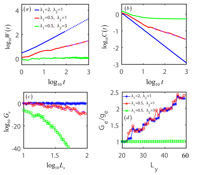
Figure 2: The evolution of (a) mean square displacement and (b) autocorrelation function averaged over $50$ samples. The particle is initially localized at $(i,j)=(\frac{L_{x}}{2},\frac{L_{y}}{2})$ with system size $L_{x}=L_{y}=400$. (c) The conductance as a function of $L_{x}$ in the unit of $e^{2}/h$ with $L_{y}=10$ fixed. (d)The conductance as a function of $L_{y}$ in the unit of $g_{e}=G_{e}(L_{y}=20)$ with $L_{x}=10$ fixed. The blue/red/green curves in (a)-(d) are in the extended, critical and localized phases, with the same values to the legend in (a). The purple dashed line in (a)-(c) is the linear fitting in the critical phase. Here $\lambda_{3}=0$.

Then we investigate the transport properties for the 2D model by contacting the sample with two leads from the left and right side in the x-direction. In the zero temperature limit and linear response regime, the conductance can be written as Mahan

$$G_{e}=\frac{e^{2}}{h}Tr[\mathbf{\Gamma}_{L}\mathbf{G}^{A}\mathbf{\Gamma}_{R}\mathbf{G}^{R}],$$ (11)

where the Green’s function $\mathbf{G}^{R}(\omega)=[\omega-\mathbf{H}-\mathbf{\Sigma}_{L}^{R}(\omega)-\mathbf{\Sigma}_{R}^{R}(\omega)]^{-1}$ and $\mathbf{G}^{A}(\omega)=[\mathbf{G}^{R}(\omega)]^{\dagger}$, and the spectral density $\mathbf{\Gamma}_{L(R)}=i(\mathbf{\Sigma}_{L(R)}^{R}-\mathbf{\Sigma}_{L(R)}^{A})$. The self energies induced by the leads are $\Sigma_{L,j1}(\omega)=\Sigma_{R,jL}(\omega)=-i\frac{\gamma}{2}$, which are energy independent and non-vanishing only at the leftmost or the rightmost column in the wide band limit.

Fig. 2(c) shows the conductance as a function of the length $L_{x}$ with $L_{y}=10$, and Fig. 2(d) displays the conductance as a function of the width $L_{y}$ with $L_{x}=10$. The blue, red and green curves are selected in the extended, critical and localized phases, with the parameters the same as Figs. 2(a)(b). In the extended phase, the transport is ballistic in the bulk, and hence the conductance is independent of length $G_{e}\sim L_{x}^{0}$ and proportional to the numbers of scattering channels and hence $G_{e}\sim L_{y}^{1}$. In the critical phase, the transport is diffusive indicating the power-law dependence of length $G_{e}\sim L_{x}^{-\alpha}$ and interestingly, also proportional to the width $G_{e}\sim L_{y}^{1}$ just like the extended phase. In the localized phase, the bulk is insulating and the conductance is exponentially decay with respect to the length $G_{e}\sim e^{-L_{x}}$ and independent of the width $G_{e}\sim L_{y}^{0}$. In all the cases, the chemical potentials (Fermi energies) are selected inside the energy band.

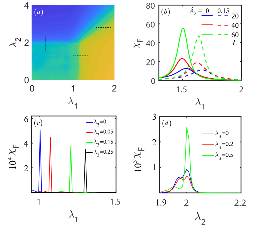
Figure 3: (a) Phase diagram of the 2D model characterized by the average fractal dimension with NNN hopping $\lambda_{3}=0.15$, and the colourmap is the same as Fig. 1(a). (b) Fidelity susceptibility as a function of $\lambda_{1}$ for different sizes with fixed $\lambda_{2}=3$. The NNN hopping $\lambda_{3}=0$ for solid lines and $\lambda_{3}=0.15$ for dashed lines. (c) Fidelity susceptibility versus $\lambda_{1}$ with $\lambda_{2}=1.25$. (d)Fidelity susceptibility versus $\lambda_{2}$ for $\lambda_{1}=0.3$. The system sizes here are $L_{x}=L_{y}=40$.

IV With NNN hopping

In this section, we discuss whether the critical phase is stable when the NNN hopping strength $\lambda_{3}$ is non-zero. The 2D model (1) with non-zero $\lambda_{3}$ cannot be separated into two 1D models. Fig. 3(a) shows the phase diagram using the average fractal dimension with $\lambda_{3}=0.15$. It can be seen there are still the extended, critical and localized phases, but the phase boundary will change.

To see how the phase boundary shift, it is convenient to calculate the fidelity susceptibility

$$\chi_{F}=-2\sum_{\alpha=1,2}\lim_{\delta\lambda_{\alpha}\rightarrow 0}\frac{\ln F_{\alpha}}{\delta\lambda_{\alpha}^{2}},$$ (12)

where the ground state fidelity $F_{\alpha}=|\langle\Psi_{g}(\lambda_{\alpha}+d\lambda_{\alpha})|\Psi_{g}(\lambda_{\alpha})\rangle|$ measures the overlap between $|\Psi_{g}(\lambda_{\alpha})\rangle$ and $|\Psi_{g}(\lambda_{\alpha}+d\lambda_{\alpha})\rangle$ Zanardi ; GuSJ ; ChenS . Near the phase transition point, the behavior of wavefunctions changes dramatically and $\chi_{F}$ will be divergent. Fig. 3(b) shows the $\chi_{F}$ as a function of $\lambda_{1}$ for different sizes with $\lambda_{2}=3$. It can be seen that without the NNN hopping $\lambda_{3}=0$, $\chi_{F}$ has a peak at $\lambda_{1}=1.5$, which gives the same phase boundary as the fractal dimension. In the presence of $\lambda_{3}$, the peak shifts to $\lambda_{1}\sim 1.63$, and in both cases, the peak will be divergent as increasing the system size. Figs. 3(c) and (d) show the fidelity susceptibility near the transition points from the critical phase to extended and localized phases, respectively, with different $\lambda_{3}$. As the increase of $\lambda_{3}$, the peak of $\chi_{F}$ shifts towards large $\lambda_{1}$ [Fig. 3(c)], while the peak of $\chi_{F}$ gives nearly the same $\lambda_{2}$ [Fig. 3(d)]. Therefore, the phase boundary between critical and extended phases and the boundary between localized and extended phases shift toward larger $\lambda_{1}$, while the phase boundary between critical and localized phases remains $\lambda_{2}=2$, as shown in Fig. 3(a).

V Experimental realization

Finally, we discuss the implementation of the 2D model (1), whose hopping strength is quasiperiodic, which is difficult to achieve in some simulated systems. Here, we discuss the implementation of this model on a a superconducting quantum processor (SQP), using the special case of $\lambda_{3}=0$ as an example. The case with $\lambda_{3}\neq 0$ can be realized in a similar manner. The SQP consists of the 2D array of $L_{x}\times L_{y}$ transmon superconducting qubits, along with $(L_{x}-1)L_{y}+(L_{y}-1)L_{x}$ tunable couplers, each positioned between every two nearest-neighbor qubits, as shown in Fig. 4(a). The effective coupling coupling $h^{x}_{i,j}$ in Eq. (1) can be described by YanF ; HengFan2021 :

$$h^{x}_{i,j}=g^{QQ}_{ij;i+1j}+\frac{g^{QC}_{ij;iji+1j}g^{QC}_{i+1j;iji+1j}}{\Delta_{ij,i+1j}},$$ (13)

which contains two parts: the first term $g^{QQ}_{ij;i+1j}$ represents the direct coupling between neighboring qubits $Q_{i,j}$ and $Q_{i+1,j}$, and the second term represents the coupling between the coupler $C_{ij,i+1j}$ and the two nearest-neighbor qubits $Q_{i,j}$ and $Q_{i+1,j}$ (see Fig. 4), where $g^{QC}_{ij;iji+1j}$ is the coupling strength between $Q_{i,j}$ and $C_{ij,i+1j}$, and $1/\Delta_{ij,i+1j}=[1/(\omega_{ij}-\omega^{C}_{ij;i+1j})+1/(\omega_{i+1j}-\omega^{C}_{ij;i+1j})]/2$ with $\omega_{ij}$ and $\omega^{C}_{ij;i+1j}$ being the corresponding frequency of the qubit $Q_{i,j}$ and the coupler $C_{ij,i+1j}$, respectively. Similarly, we can obtain the hopping strength $h^{y}_{i,j}$ in the $y$-direction. The on-site quasiperiodic potential $V_{i,j}$ is represented as:

$$\begin{split}V_{i,j}=&\omega_{ij}+\frac{(g_{ij;iji+1j}^{QC})^{2}}{\omega_{ij}-\omega_{ij;i+1j}^{c}}+\frac{(g_{ij;iji-1j}^{QC})^{2}}{\omega_{ij}-\omega_{ij;i-1j}^{c}}\\ +&\frac{(g_{ij;ijij+1}^{QC})^{2}}{\omega_{ij}-\omega_{ij;ij+1}^{c}}+\frac{(g_{ij;ijij-1}^{QC})^{2}}{\omega_{ij}-\omega_{ij;ij-1}^{c}}.\end{split}$$ (14)

By tuning the frequencies of qubits and couplers, we can obtain the desired forms and strengths of the nearest-neighbor hopping and on-site potential.

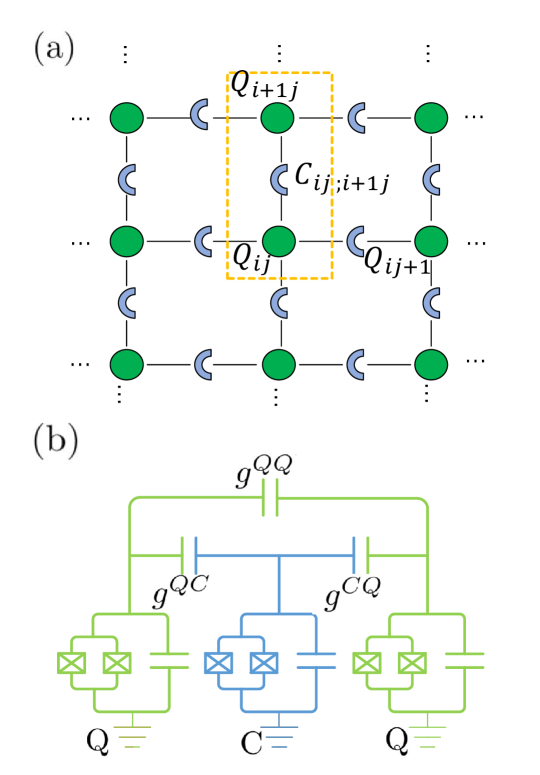
Figure 4: (a) Schematic representation of the 2D model (1) with $\lambda_{3}=0$ on the superconducting quantum processor, which consists of $L_{x}\times L_{y}$ transmon superconducting qubits and $(L_{x}-1)L_{y}+(L_{y}-1)L_{x}$ tunable couplers. (b) The circuit diagram of neighboring qubits and the coupler between them.

By manipulating both qubits and couplers, we can experimentally observe the dynamics of different phases in this model. Therefore, we can experimentally detect the critical phase and transitions between different phases based on their dynamic properties.

VI Conclusion and Discussion

We have introduced a 2D quasiperiodic model exhibiting a critical phase and provided its phase diagram. We adapted a finite-size scaling method to effectively determine the phase boundaries of this model and obtain critical exponents. Additionally, we explored the properties of the critical, extended and localized phases in terms of wave packet diffusion and transport in this 2D system, and examined the changes of phase boundaries in the phase diagram induced by the introduction of NNN hopping through calculations of fidelity susceptibility. Finally, we discussed the realization of this model in superconducting circuits. Our work paves the way for searching the critical phase in 2D systems.

Recent research has revealed the presence of novel anomalous MEs in 1D systems. Unlike conventional MEs that separate extended states from localized states, these MEs delineate the critical state from either extended or localized states XDeng2019 ; Wang2022 ; XCZhou ; LiuT . Our findings suggest that since critical phases can be extended from one dimension to two dimension, these novel MEs can also be extended to two dimension, warranting further investigation in the future.

- (1) P. W. Anderson, Phys. Rev. 109, 1492 (1958).
- (2) P. A. Lee and T. V. Ramakrishnan, Disordered electronic systems, Rev. Mod. Phys. 57, 287 (1985).
- (3) F. Evers and A. D. Mirlin, Anderson transitions, Rev. Mod. Phys. 80, 1355 (2008).
- (4) B. Kramer and A. MacKinnon, Localization: theory and experiment, Rep. Prog. Phys. 56, 1469 (1993).
- (5) C. M. Soukoulis and E. N. Economou, Localization in One-Dimensional Lattices in the Presence of Incommensurate Potentials, Phys. Rev. Lett. 48, 1043 (1981).
- (6) S. Das Sarma, S. He, and X. C. Xie, Mobility edge in a model one-dimensional potential, Phys. Rev. Lett. 61, 2144 (1988).
- (7) J. Biddle, B. Wang, D. J. Priour, Jr.,and S. Das Sarma, Localization in one-dimensional incommensurate lattices beyond the Aubry-André model, Phys. Rev. A 80, 021603 (2009); J. Biddle and S. Das Sarma, Predicted mobility edges in one-dimensional incommensurate optical lattices: an exactly solvable model of Anderson localization, Phys. Rev. Lett. 104, 070601 (2010).
- (8) X. Li, X. Li, and S. Das Sarma, Mobility edges in one dimensional bichromatic incommensurate potentials, Phys. Rev. B 96, 085119 (2017); D. Vu and S. Das Sarma, Generic mobility edges in several classes of duality-breaking one-dimensional quasiperiodic potentials, Phys. Rev. B 107, 224206 (2023).
- (9) H. Yao, H. Khoudli, L. Bresque, and L. Sanchez-Palencia, Critical behavior and fractality in shallow one-dimensional quasiperiodic potentials, Phys. Rev. Lett. 123, 070405 (2019).
- (10) S. Ganeshan, J. H. Pixley, and S. Das Sarma, Nearest neighbor tight binding models with an exact mobility edge in one dimension, Phys. Rev. Lett. 114, 146601 (2015).
- (11) Y. Wang, X. Xia, L. Zhang, H. Yao, S. Chen, J. You, Q. Zhou, and X.-J. Liu, One dimensional quasiperiodic mosaic lattice with exact mobility edges, Phys. Rev. Lett. 125, 196604 (2020).
- (12) X. Deng, S. Ray, S. Sinha, G. Shlyapnikov, and L. Santos, One-dimensional quasicrystals with power-law hopping, Phys. Rev. Lett. 123, 025301 (2019).
- (13) M. Gonçalves, B. Amorim, E. V. Castro, and P. Ribeiro, Hidden dualities in 1D quasiperiodic lattice models, SciPost Phys. 13, 046 (2022); M. Gonçalves, B. Amorim, E. V. Castro, and P. Ribeiro, Renormalization-Group Theory of 1D quasiperiodic lattice models with commensurate approximants, Phys. Rev. B 108, L100201 (2023); M. Gonçalves, B. Amorim, E. V. Castro, and P. Ribeiro, Critical phase dualities in 1D exactly-solvable quasiperiodic models, Phys. Rev. Lett. 131, 186303 (2023).
- (14) Y. Liu, Z. Wang, C. Yang, J. Jie, and Y. Wang, Dissipation-Induced Extended-Localized Transition, Phys. Rev. Lett. 132, 216301 (2024).
- (15) G. Roati, C. D’Errico, L. Fallani, M. Fattori, C. Fort, M. Zaccanti, G. Modugno, M. Modugno, and M. Inguscio, Anderson localization of a non-interacting Bose-Einstein condensate, Nature (London) 453, 895 (2008).
- (16) H. P. Lüschen, S. Scherg, T. Kohlert, M. Schreiber, P. Bordia, X. Li, S. D. Sarma, and I. Bloch, Single-particle mobility edge in a one-dimensional quasiperiodic optical lattice, Phys. Rev. Lett. 120, 160404 (2018); T. Kohlert, S. Scherg, X. Li, H. P. Lüschen, S. D. Sarma, I. Bloch, and M. Aidelsburger, Observation of many-body localization in a one-dimensional system with single-particle mobility edge, Phys. Rev. Lett. 122, 170403 (2019).
- (17) F. A. An, E. J. Meier, and B. Gadway, Engineering a flux-dependent mobility edge in disordered zigzag chains, Phys. Rev. X 8, 031045 (2018); F. A. An, K. Padavić, E. J. Meier, S. Hegde, S. Ganeshan, J. H. Pixley, S. Vishveshwara, and B. Gadway, Observation of tunable mobility edges in generalized Aubry-André lattices, Phys. Rev. Lett. 126, 040603 (2021).
- (18) Y. Wang, J.-H. Zhang, Y. Li, J. Wu, W. Liu, F. Mei, Y. Hu, L. Xiao, J. Ma, C. Chin, and S. Jia, Observation of Interaction-Induced Mobility Edge in an Atomic Aubry-André Wire, Phys. Rev. Lett. 129, 103401 (2022).
- (19) N. Rosenzweig and C. E. Porter, “Repulsion of Energy Levels” in Complex Atomic Spectra, Phys. Rev. 120, 1698 (1960).
- (20) H. Kunz and B. Shapiro, Transition from Poisson to Gaussian unitary statistics: The two-point correlation function, Phys. Rev. E 58, 400 (1998).
- (21) T. Xiao, D. Xie, Z. Dong, T. Chen, W. Yi, and B. Yan, Observation of topological phase with critical localization in a quasi-periodic lattice, Science Bulletin 66, 2175 (2021).
- (22) T. Shimasaki, M. Prichard, H. E. Kondakci, J. Pagett, Y. Bai, P. Dotti, A. Cao, T.-C. Lu, T. Grover, and D. M. Weld, Anomalous localization and multifractality in a kicked quasicrystal, arXiv:2203.09442.
- (23) H. Li, Y.-Y. Wang, Y.-H. Shi, K. Huang, X. Song, G.-H. Liang, Z.-Y. Mei, B. Zhou, H. Zhang, J.-C. Zhang, et al., Observation of critical phase transition in a generalized Aubry-André-Harper model with superconducting circuits, npj Quantum Information 9, 40 (2023).
- (24) Y. Wang, L. Zhang, S. Niu, D. Yu, and X.-J. Liu, Realization and detection of non-ergodic critical phases in optical Raman lattice, Phys. Rev. Lett. 125, 073204 (2020).
- (25) Y. Hatsugai and M. Kohmoto, Energy spectrum and the quantum Hall effect on the square lattice with next-nearest-neighbor hopping, Phys. Rev. B 42, 8282 (1990); J. H. Han, D. J. Thouless, H. Hiramoto, and M. Kohmoto, Critical and bicritical properties of Harper’s equation with next-nearest-neighbor coupling, Phys. Rev. B 50, 11365 (1994).
- (26) Y. Wang, C. Cheng, X.-J. Liu, and D. Yu, Many-body critical phase: extended and nonthermal, Phys. Rev. Lett. 126, 080602 (2021).
- (27) M. Gonçalves, B. Amorim, F. Riche, E. V. Castro, and P. Ribeiro, Incommensurability enabled quasi-fractal order in 1D narrow-band moiré systems, arXiv:2305.03800.
- (28) T. Geisel, R. Ketzmerick, and G. Petschel, New class of level statistics in quantum systems with unbounded diffusion, Phys. Rev. Lett. 66,1651 (1991).
- (29) S. Y. Jitomirskaya, Metal-insulator transition for the almost mathieu operator, Ann. Math. 3, 150 (1999).
- (30) T. C. Halsey, M. H. Jensen, L. P. Kadanoff, I. Procaccia, and B. I. Shraiman, Fractal measures and their singularities: The characterization of strange sets, Phys. Rev. A 33, 1141 (1986).
- (31) A. D. Mirlin, Y. V. Fyodorov, A. Mildenberger, and F. Evers, Exact relations between multifractal exponents at the Anderson transition, Phys. Rev. Lett. 97, 046803 (2006).
- (32) H. Hiramoto and S. Abe, Dynamics of an Electron in Quasiperiodic Systems. II. Harper’s Model, J. Phys. Soc. Jpn. 57, 1365 (1988).
- (33) R. Ketzmerick, K. Kruse, S. Kraut, and T. Geisel, What determines the spreading of a wave packet?, Phys. Rev. Lett. 79, 1959 (1997).
- (34) A. Jagannathan, The Fibonacci quasicrystal: Case study of hidden dimensions and multifractality, Rev. Mod. Phys. 93, 045001 (2021).
- (35) G. T. Landi, D. Poletti, and G. Schaller, Nonequilibrium boundary-driven quantum systems: Models, methods, and properties, Rev. Mod. Phys. 94, 045006 (2022).
- (36) M. Saha, S. K. Maiti, and A. Purkayastha, Anomalous transport through algebraically localized states in one dimension, Phys. Rev. B 100, 174201 (2019); M. Saha, B. P. Venkatesh, and B. K. Agarwalla, Quantum transport in quasiperiodic lattice systems in the presence of Büttiker probes, Phys. Rev. B 105, 224204 (2022).
- (37) A. Purkayastha, A. Dhar, and M. Kulkarni, Nonequilibrium phase diagram of a one-dimensional quasiperiodic system with a single-particle mobility edge, Phys. Rev. B 96, 180204(R) (2017).
- (38) Y. Wang, L. Zhang, W. Sun, T.-F. J. Poon, and X.-J. Liu, Quantum phase with coexisting localized, extended, and critical zones, Phys. Rev. B 106, L140203 (2022).
- (39) Z. Fan, G.-W. Chern. and S.-Z. Lin, Enhanced superconductivity in quasiperiodic crystals, Phys. Rev. Res. 3, 023195 (2021).
- (40) X. Zhang and M. S. Foster, Enhanced amplitude for superconductivity due to spectrum-wide wave function criticality in quasiperiodic and power-law random hopping models, Phys. Rev. B 106, L180503 (2022).
- (41) J. Mayoh and A. M. García-García, Global critical temperature in disordered superconductors with weak multifractality, Phys. Rev. B 92, 174526 (2015).
- (42) M. V. Feigel’man, L. B. Ioffe, V. E. Kravtsov, and E. A. Yuzbashyan, Eigenfunction Fractality and Pseudogap State near the Superconductor-Insulator Transition, Phys. Rev. Lett. 98, 027001 (2007); M. V. Feigel’man, L. B. Ioffe, V. E. Kravtsov, and E. Cuevas, Fractal superconductivity near localization threshold, Ann. Phys. (NY). 325, 1390 (2010).
- (43) Q. Marsal and A. M. Black-Schaffer, Enhanced Quantum Metric due to Vacancies in Graphene, Phys. Rev. Lett. 133, 026002 (2024).
- (44) A. Szabó and U. Schneider, Mixed spectra and partially extended states in a two-dimensional quasiperiodic model, Phys. Rev. B 101, 014205 (2020).
- (45) A. Štrkalj, E. V. H. Doggen, and C. Castelnovo, Coexistence of localization and transport in many-body two-dimensional Aubry-André models, Phys. Rev. B 106, 184209 (2022).
- (46) H.-J. Li, J.-P. Dou, and G. Huang, Realization of two-dimensional Aubry-André localization of light waves via electromagnetically induced transparency, Phys. Rev. A 89, 033843 (2014).
- (47) P. Bordia, H. Lüschen, S. Scherg, S. Gopalakrishnan, M. Knap, U. Schneider, and I. Bloch, Probing Slow Relaxation and Many-Body Localization in Two-Dimensional Quasiperiodic Systems, Phys. Rev. X 7, 041047 (2017).
- (48) N. A. Khan, S. Ye, Z. Zhou, S. Cheng, and G. Xianlong, Chebyshev polynomial approach to Loschmidt echo: Application to quench dynamics in two-dimensional quasicrystals, Phys. Rev. E 109, 065311 (2024).
- (49) Y. Wang, L. Zhang, Y. Wan, Y. He, and Y. Wang, Two dimensional vertex-decorated Lieb lattice with exact mobility edges and robust flat bands, Phys. Rev. B 107, L140201 (2023).
- (50) M. Rossignolo and L. Dell’Anna, Localization transitions and mobility edges in coupled Aubry-André chains, Phys. Rev. B 99, 054211 (2019).
- (51) Z.-H. Xu, X. Xia, and S. Chen, Exact mobility edges and topological phase transition in two-dimensional non-Hermitian quasicrystals, Sci. China Phys. Mech. Astron. 65, 227211 (2022).
- (52) C. W. Duncan, Critical states and anomalous mobility edges in two-dimensional diagonal quasicrystals, Phys. Rev. B 109, 014210 (2024).
- (53) We note that we are considering a system where the potential is quasiperiodic, but the spatial structure is periodic.
- (54) Y. Takada, K. Ino, and M. Yamanaka, Statistics of spectra for critical quantum chaos in one-dimensional quasiperiodic systems, Phys. Rev. E 70, 066203 (2004).
- (55) F. Liu, S. Ghosh, and Y. D. Chong, Localization and adiabatic pumping in a generalized Aubry-André-Harper model, Phys. Rev. B 91, 014108 (2015).
- (56) G. G. Batrouni and R. T. Scalettar, Quantum Phase Transitions, in Ultracold Gases and Quantum Information (Oxford University Press, Oxford, 2011).
- (57) S. Sachdev, Quantum Phase Transitions (Cambridge University Press, New York, 2011).
- (58) Y. Hashimoto, K. Niizeki, and Y. Okabe, A finite-size scaling analysis of the localization properties of one-dimensional quasiperiodic systems, J. Phys. A: Math. Gen. 25, 5211 (1992).
- (59) Y. Wang, Y. Wang, and S. Chen, Spectral statistics, finite-size scaling and multifractal analysis of quasiperiodic chain with p-wave pairing, Eur. Phys. J. B 89, 254 (2016).
- (60) The method for determining the error bars primarily follows Appendix B of the paper by C. L. Bertrand and A. M. García-García, Anomalous Thouless energy and critical statistics on the metallic side of the many-body localization transition, Phys. Rev. B 94, 144201 (2016).
- (61) J. Zhong, R. B. Diener, D. A. Steck, W. H. Oskay, M. G. Raizen, E. W. Plummer, Z. Zhang, and Q. Niu, Shape of the Quantum Diffusion Front, Phys. Rev. Lett 86, 2485 (2001).
- (62) R. Ketzmerick, G. Petschel, and T. Geisel, Slow decay of temporal correlations in quantum systems with Cantor spectra, Phys. Rev. Lett. 69, 695 (1992).
- (63) J. X. Zhong and R. Mosseri, Quantum dynamics in quasiperiodic systems, J. Phys.: Condens. Matter 7, 8383(1995).
- (64) G. D. Mahan, Many-Particle Physics (Kluwer Academic/Plenum, New York, 2000).
- (65) P. Zanardi, P. Glorda, and M. Cozzini, Information-Theoretic Differential Geometry of Quantum Phase Transitions, Phys. Rev. Lett. 99, 100603 (2007).
- (66) W.-L. You, Y.-W. Li, and S.-J. Gu, Fidelity, dynamic structure factor, and susceptibility in critical phenomena, Phys. Rev. E 76, 022101 (2007).
- (67) S. Chen, L. Wang, Y. Hao, and Y. Wang, Intrinsic relation between ground-state fidelity and the characterization of a quantum phase transition, Phys. Rev. A 77, 032111 (2008).
- (68) F. Yan, P. Krantz, Y. Sung, M. Kjaergaard, D. L. Campbell, T. P. Orlando, S. Gustavsson, and W. D. Oliver, Tunable Coupling Scheme for Implementing High-Fidelity Two-Qubit Gates, Phys. Rev. Appl. 10, 1 (2018).
- (69) Y.-H. Shi, R.-Q. Yang, Z. Xiang, Z.-Y. Ge, H. Li, Y.-Y. Wang, K. Huang, Y. Tian, X. Song, D. Zheng, K. Xu, R.-G. Cai, and H. Fan, On-chip black hole: Hawking radiation and curved spacetime in a superconducting quantum circuit with tunable couplers, Nat. Comm. 14, 3263 (2023).
- (70) X.-C. Zhou, Y. Wang, T.-F. J. Poon, Q. Zhou, and X.-J. Liu, Exact new mobility edges between critical and localized states, Phys. Rev. Lett. 131, 176401 (2023).
- (71) T. Liu, X. Xia, S. Longhi, L. Sanchez-Palencia, Anomalous mobility edges in one-dimensional quasiperiodic models, SciPost Phys. 12, 027 (2022).