Nevanlinna Theory on Complete Kähler Connected Sums With Non-parabolic Ends

Abstract.

Motivated by invalidness of Liouville property for harmonic functions on the connected sum $\#^{\vartheta}\mathbb{C}^{m}$ with $\vartheta\geq 2,$ we study Nevanlinna theory on a complete Kähler connected sum

$$M=M_{1}\#\cdots\#M_{\vartheta}$$

with $\vartheta$ non-parabolic ends. Based on the global Green function method, we extend the second main theorem of meromorphic mappings to $M.$ As a consequence, we obtain a Picard’s little theorem provided that all $M_{j}^{,}s$ have non-negative Ricci curvature, which states that every meromorphic function on $M$ reduces to a constant if it omits three distinct values. In particular, it implies that Cauchy-Riemann equation supports a rigidity of Liouville property as an invariant under connected sums.

1. Introduction

1.1. Motivation

Why should we study Nevanlinna theory on a complex manifold with ends (i.e., a connected sum of complex manifolds)? An intrinsic motivation is that Liouville property fails for harmonic functions on such geometric objects. As we all know, each bounded harmonic function on $\mathbb{C}^{m}$ is a constant. However, it doesn’t hold on the connected sum $\mathbb{C}^{m}\#\mathbb{C}^{m}$ supporting a Kähler structure. As early as 1979, Kuz’menko-Molchanov [33] considered the connected sum $\mathbb{R}^{m}\#\mathbb{R}^{m}$ as an example of a manifold (see Fig. 1), where Liouville property fails for harmonic functions. Later, Grigor’yan-Saloff-Coste [23, 25] observed this phenomenon also on a more general connected sum of complete weighted manifolds with non-negative Ricci curvature, where they constructed a non-constant bounded harmonic function using the heat kernel. In order to serve this paper, we give an example of several complex variables which is a special case of Grigor’yan-Saloff-Coste’s construction (see [25], Proposition 6.3).

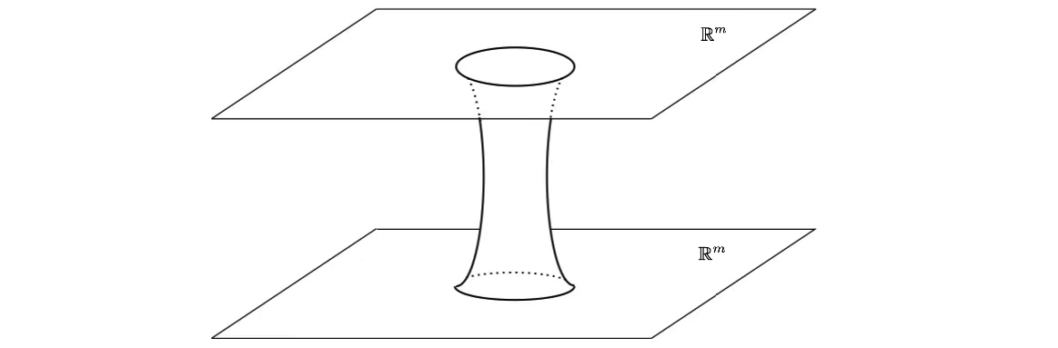
Figure 1. $\mathbb{R}^{m}\#\mathbb{R}^{m}$

Let $\#^{\vartheta}\mathbb{C}^{m}$ denote the connected sum of $\vartheta$ copies of $\mathbb{C}^{m}$ which does support a Kähler structure. Precisely, there exists a non-compact subset $K\subset\#^{\vartheta}\mathbb{C}^{m}$ (with nonempty interior) such that $\#^{\vartheta}\mathbb{C}^{m}\setminus K$ is a disjoint union of $\vartheta$ open subsets $E_{1},\cdots,E_{\vartheta},$ where each $E_{j}$ is (analytically) isometric to $\mathbb{C}^{m}\setminus K_{j}$ for some compact subset $K_{j}\subset\mathbb{C}^{m}.$ In fact, each $E_{j}$ is identified with $\mathbb{C}^{m}\setminus K_{j}.$ We shall refer to $K$ as the central part of $\#^{\vartheta}\mathbb{C}^{m},$ and refer to $E_{1},\cdots,E_{\vartheta}$ as the ends of $\#^{\vartheta}\mathbb{C}^{m}.$ Note that $\mathbb{C}^{m}=\#^{\vartheta}\mathbb{C}^{m}$ with $\vartheta=1.$ For $x\in\#^{\vartheta}\mathbb{C}^{m},$ set

$$|x|=\sup_{y\in K}d(x,y),$$

where $d(x,y)$ is the Riemannian distance between $x,y.$ Fix a reference point $o\in\#^{\vartheta}\mathbb{C}^{m}.$ Let $B(r)$ denote the geodesic ball centered at $o$ with radius $r$ in $\#^{\vartheta}\mathbb{C}^{m}.$ Set

$$V_{0}(r)=\mathop{\mathrm{min}}_{1\leq j\leq\vartheta}V_{j}(r)$$

with

$$V_{j}(r)={\rm{Vol}}\left(B(r)\cap(K\cup E_{j})\right),\ \ \ \ j=1,\cdots,\vartheta.$$

Again, put

$$i_{x}=\begin{cases}0,\ &x\in K;\\ j,\ &x\in E_{j}\ \text{for some}\ j.\end{cases}$$

Let $u,v$ be two non-negative functions defined on the same domain. We then write $u\simeq v,$ if there are constants $\alpha,\beta>0$ such that $\alpha v\leq u\leq\beta v.$ Put $w^{+}=\max\{w,0\},$ i.e., the positive part of a real function $w.$ Let $\mathscr{H}(\#^{\vartheta}\mathbb{C}^{m})$ denote the space of harmonic functions on $\#^{\vartheta}\mathbb{C}^{m},$ and $\mathscr{H}^{\flat}(\#^{\vartheta}\mathbb{C}^{m})$ denote the space of bounded harmonic functions on $\#^{\vartheta}\mathbb{C}^{m},$ and $\mathscr{H}^{+}(\#^{\vartheta}\mathbb{C}^{m})$ denote the linear space spanned by the set of positive harmonic functions on $\#^{\vartheta}\mathbb{C}^{m}.$

The following theorem is due to Grigor’yan-Saloff-Coste [25], Li-Tam[35] and Sung-Tam-Wang [49].

Theorem A ([25], Proposition 6.3).

Liouville property fails for $\mathscr{H}(\#^{\vartheta}\mathbb{C}^{m})$ if $\vartheta\geq 2.$ Moreover, there exists a positive harmonic function $h\in\mathscr{H}(\#^{\vartheta}\mathbb{C}^{m})$ such that

$$h(x)\simeq 1+\left(\int_{1}^{|x|}\frac{dt}{V_{i_{x}}(\sqrt{t})}\right)^{+}.$$

Actually, the Liouville property of a harmonic function is not only close to its own feature, but related to the structure of its defining domain. Taking a connected sum breaks the old structure on $\mathbb{C}^{m}$ and creates a new structure on $\#^{\vartheta}\mathbb{C}^{m},$ this change (in topology) affects the stability of Liouville property. As early as 1987, Li-Tam [35, 36] had demonstrated that the dimension of the space of bounded harmonic functions on complete non-compact Riemannian manifolds which have non-negative sectional curvature outside a compact set is related to the number of ends of the manifolds. Apply their results in [35], we obtain

$$\dim\mathscr{H}^{\flat}(\#^{\vartheta}\mathbb{C}^{m})=\dim\mathscr{H}^{+}(\#^{\vartheta}\mathbb{C}^{m})=\vartheta.$$

Therefore, Liouville property is not an invariant under a connected sum for a general harmonic function. It is asked that on which conditions a harmonic function must possess the Liouville property. Is it possible for any harmonic function satisfying $C$-$R$ equation? In other words, is Liouville property rigid under connected sums for holomorphic functions?

Let $\mathscr{O}(\#^{\vartheta}\mathbb{C}^{m})$ denote the Abelian ring of holomorphic functions on $\#^{\vartheta}\mathbb{C}^{m},$ which is a subspace of $\mathscr{H}(\#^{\vartheta}\mathbb{C}^{m}).$ The following question is natural.

Question 1.

Is Liouville property valid for $\mathscr{O}(\#^{\vartheta}\mathbb{C}^{m})$?

The famous Picard’s little theorem claims that any meromorphic function on $\mathbb{C}^{m}$ must be a constant if it omits three distinct values. It is obvious that this theorem generalizes the Liouville’s theorem. In this point of view, what about a meromorphic function on a connected sum? Specifically, we propose a deeper question as follows.

Question 2.

Does Picard’s little theorem hold for $\mathscr{O}(\#^{\vartheta}\mathbb{C}^{m})$?

The main purpose in the paper is to investigate Nevanlinna theory [43] on a complete Kähler connected sum with non-parabolic ends (i.e., a complete Kähler manifold with non-parabolic ends). We will prove that $C$-$R$ equation supports a rigidity of Liouville property that is an invariant under connected sums, which provides a positive answer to Question 1. Equivalently, one has

$$\dim\mathscr{O}^{\flat}(\#^{\vartheta}\mathbb{C}^{m})=1,$$

where $\mathscr{O}^{\flat}(\#^{\vartheta}\mathbb{C}^{m})$ is the space of bounded holomorphic functions on $\#^{\vartheta}\mathbb{C}^{m}.$ In fact, we shall prove a defect relation in Nevanlinna theory, which provides a positive answer to Question 2 for $m\geq 2.$ We should remark that Questions 1, 2 for $m=1$ also have a positive answer. Since $\#^{\vartheta}\mathbb{C}$ is a Riemann surface with $\vartheta$ parabolic ends that is not a non-parabolic manifold, we don’t intend to discuss this case in the present paper.

1.2. Main Results

We give a brief introduction to the main results in this paper. Let

$$M=M_{1}\#\cdots\#M_{\vartheta}=\left(K;\{M_{j}\}_{j=1}^{\vartheta};\{E_{j}\}_{j=1}^{\vartheta}\right)$$

be a complete Kähler connected sum with $\vartheta$ non-parabolic ends, where all $M_{j}^{,}s$ are complete non-compact Kähler manifolds satisfying $(PH)$ (see Property 2.5 in Section 2.2 and Definition 3.4 in Section 3.2). Note that $E_{j}^{,}s$ are the ends of $M$ and $K$ is the central part of $M$ (see definition in Section 2.3). Fix a reference point $o$ in the interior of $K.$ Let $\rho(x)$ be the Riemannian distance function of $x$ from $o,$ and $V(r)$ be the Riemannian volume of geodesic ball $B(r)$ centered at $o$ with radius $r$ in $M.$ Set

$$V_{\rm min}(r)=\mathop{\mathrm{min}}_{1\leq j\leq\vartheta}V_{j}(r),\ \ \ \ V_{\max}(r)=\max_{1\leq j\leq\vartheta}V_{j}(r)$$

with

$$V_{j}(r)={\rm{Vol}}\left(B(r)\cap(K\cup E_{j})\right),\ \ \ \ j=1,\cdots,\vartheta.$$

Let $X$ be a complex projective manifold of complex dimension not greater than that of $M.$ We can put a positive line bundle $L$ over $X.$ Let $f:M\to X$ be a meromorphic mapping. With the two-sided bounds of the heat kernel of $M,$ we can construct a family $\{\Delta(r)\}_{r>0}$ of exhaustive precompact domains for $M$ (see definition in Section 3.3). Taking a divisor $D\in|L|.$ On $\Delta(r),$ we can define Nevanlinna’s functions $T_{f}(r,L),m_{f}(r,D),\overline{N}_{f}(r,D)$ and $T(r,\mathscr{R}),$ where $\mathscr{R}:=-dd^{c}\log\det(g_{i\bar{j}})$ denotes the Ricci form associated to the metric $g=(g_{i\bar{j}})$ of $M$ (see details in Section 3.3). Set

(1) $$\Xi(r)=\sup_{x\in\partial\Delta(r)}\frac{\rho(x)\displaystyle\int_{0}^{\infty}\frac{e^{-\frac{\rho(x)^{2}}{Bt}}}{V_{\rm min}(\sqrt{t})}\frac{dt}{t}}{r\displaystyle\int_{0}^{\infty}\frac{e^{-\frac{r^{2}}{At}}}{V_{\max}(\sqrt{t})}\frac{dt}{t}}.$$

With these notations, we establish a second main theorem as follows.

Theorem 1.1.

Let $M=M_{1}\#\cdots\#M_{\vartheta}$ be a complete Kähler connected sum with $\vartheta$ non-parabolic ends, where all $M_{j}^{,}s$ are non-compact satisfying $(PH).$ Let $X$ be a complex projective manifold of complex dimension not greater than that of $M.$ Let $D\in|L|$ be a reduced divisor of simple normal crossing type, where $L$ is a positive line bundle over $X.$ Let $f:M\rightarrow X$ be a differentiably non-degenerate meromorphic mapping. Then for any $\delta>0,$ there exists a subset $E_{\delta}\subset(0,\infty)$ of finite Lebesgue measure such that

$$T_{f}(r,L)+T_{f}(r,K_{X})+T(r,\mathscr{R})-\overline{N}_{f}(r,D)$$

$$\leq O\left(\log^{+}T_{f}(r,L)+\delta\log^{+}\left(r\int_{0}^{\infty}\frac{e^{-\frac{r^{2}}{At}}}{V_{\max}(\sqrt{t})}\frac{dt}{t}\right)^{-1}+\log^{+}\Xi(r)\right)$$

holds for all $r>0$ outside $E_{\delta}.$

By Li-Yau’s argument [34], the non-negativeness of Ricci curvature of all $M_{j}^{,}s$ implies the two-sided heat kernel bounds $(HK)$ in Property 2.5 which is equivalent to $(PH)$ due to Theorem 2.6 in Section 2.2. When all $M_{j}^{,}s$ have non-negative Ricci curvature and $M$ is homogeneous (see Definition 7.1 in Section 7), we estimate the last two error terms in the above inequality and prove the following result.

Corollary 1.2.

Let $M=M_{1}\#\cdots\#M_{\vartheta}$ be a complete Kähler connected sum with $\vartheta$ non-parabolic ends, where all $M_{j}^{,}s$ are non-compact with non-negative Ricci curvature. Let $X$ be a complex projective manifold of complex dimension not greater than that of $M.$ Let $D\in|L|$ be a reduced divisor of simple normal crossing type, where $L$ is a positive line bundle over $X.$ Let $f:M\rightarrow X$ be a differentiably non-degenerate meromorphic mapping. Assume that $M$ is homogeneous. Then for any $\delta>0,$ there exists a subset $E_{\delta}\subset(0,\infty)$ of finite Lebesgue measure such that

$$T_{f}(r,L)+T_{f}(r,K_{X})+T(r,\mathscr{R})$$

$$\leq \overline{N}_{f}(r,D)+O\left(\log^{+}T_{f}(r,L)+\delta\log^{+}\frac{V(r)}{r}\right)$$

holds for all $r>0$ outside $E_{\delta}.$

The conditions in Corollary 1.2 imply that $T(r,\mathscr{R})$ is bounded from below by a constant and $V(r)\leq O(r^{2\dim_{\mathbb{C}}M})$ as $r\to\infty.$ Set

$$\mathfrak{S}(r)=\inf_{x\in\Delta(r)}S_{c}(x),$$

where $S_{c}$ is the scalar curvature of $M.$ We further prove that

Corollary 1.3.

Let $M$ be a non-parabolic complete non-compact Kähler manifold with non-negative Ricci curvature. Let $X$ be a complex projective manifold of complex dimension not greater than that of $M.$ Let $D\in|L|$ be a reduced divisor of simple normal crossing type, where $L$ is a positive line bundle over $X.$ Let $f:M\rightarrow X$ be a differentiably non-degenerate meromorphic mapping. Then for any $\delta>0,$ there exists a subset $E_{\delta}\subset(0,\infty)$ of finite Lebesgue measure such that

$$T_{f}(r,L)+T_{f}(r,K_{X}) \leq \overline{N}_{f}(r,D)-\frac{\mathfrak{S}(r)r^{2}}{4\dim_{\mathbb{C}}M}+O\left(\log^{+}T_{f}(r,L)+\delta\log r\right)$$

holds for all $r>0$ outside $E_{\delta}.$

We consider some defect relations. The simple defect $\bar{\delta}_{f}(D)$ and notation $[c_{1}(K_{X}^{*})/c_{1}(L)]$ (see Carlson-Griffiths [7]) are defined respectively by

$$\bar{\delta}_{f}(D) = 1-\limsup_{r\rightarrow\infty}\frac{\overline{N}_{f}(r,D)}{T_{f}(r,L)},$$

$$\left[\frac{c_{1}(K_{X}^{*})}{c_{1}(L)}\right]=\inf\left\{s\in\mathbb{R}:\ \omega\leq s\eta;\ \ ^{\exists}\eta\in c_{1}(L),\ ^{\exists}\omega\in c_{1}(K^{*}_{X})\right\}.$$

Let $\mathscr{O}(M)$ be the Abelian ring of holomorphic functions on $M.$ We obtain a defect relation which answers Question 2 ($m\geq 2$) affirmatively.

Corollary 1.4.

Assume the same conditions as in Corollary $\ref{corr4}.$ Then

$$\bar{\delta}_{f}(D)\leq\left[\frac{c_{1}(K_{X}^{*})}{c_{1}(L)}\right].$$

Hence, every meromorphic function on $M$ reduces to a constant if it omits three distinct values. In particular, Liouville property is valid for $\mathscr{O}(M).$

Set

$$\mu_{f}(L)=\mu_{f}(c_{1}(L,h))=\frac{1}{4\dim_{\mathbb{C}}M}\liminf_{r\rightarrow\infty}\frac{\mathfrak{S}(r)r^{2}}{T_{f}(r,L)}.$$

Corollary 1.5.

Assume the same conditions as in Corollary $\ref{corr2}.$ Then

$$\bar{\delta}_{f}(D)\leq\left[\frac{c_{1}(K_{X}^{*})}{c_{1}(L)}\right]-\mu_{f}(L).$$

Hence, every meromorphic function $f$ on $M$ reduces to a constant if it omits $\max\{3-[\mu_{f}(\omega_{FS})],0\}$ distinct values, where $\omega_{FS}$ is the Fubini-Study form on $\mathbb{P}^{1}(\mathbb{C})$ and $[\mu_{f}(\omega_{FS})]$ denotes the maximal integer not greater than $\mu_{f}(\omega_{FS}).$ In particular, Liouville property is valid for $\mathscr{O}(M).$

Furthermore, some other results are included in Section 8.2. For example, we obtain a second main theorem on complete Kähler manifolds which have either asymptotically non-negative sectional curvature or non-negative Ricci curvature outside a compact set (see Theorems 8.6 and 8.9 in Section 8.2).

2. Preliminaries

For the reader’s convenience, we outline some facts concerning connected sums of Riemannian manifolds and their heat kernel estimates. Throughout the paper, unless otherwise specified, a manifold is always meant boundless. We refer the reader to [23, 25, 34, 51, 53] for more details.

2.1. Weighted Manifolds

Let $(M,g)$ be a Riemannian manifold with boundary $\delta M$ (which may be empty). Fix a positive smooth function $\sigma$ on $M.$ We define a measure $\mu$ on $M$ by

$$d\mu=\sigma^{2}dv,$$

where $dv$ is the Riemannian measure (i.e., the Riemannian volume element) on $M.$ We call the pair $(M,\mu)=(M,g,\mu)$ a weighted manifold. We introduce some notations and facts from Riemannian geometry as follows.

Let $B(x,r)$ denote the geodesic ball centered at $x$ with radius $r$ in $M.$ Set

$$V(x,r)=\mu(B(x,r)),$$

which is called the $\mu$-volume of $B(x,r).$ Evidently, $V(x,r)$ is the Riemannian volume of $B(x,r)$ when $\sigma\equiv 1.$ We say that $M$ is complete if the metric space $(M,d)$ is complete, here $d$ is the Riemannian distance on $M$ induced by the metric $g.$ When $\delta M=\emptyset,$ a well-known fact states that $M$ is complete if and only if $M$ is geodesically complete (i.e., the maximal defining interval of any geodesic in $M$ is $\mathbb{R}$).

For any smooth function $u$ on $M,$ the gradient $\nabla u$ is a unique vector field defined by $g(\nabla u,X)=du(X)$ for each smooth vector field $X$ on $M.$ Locally, $\nabla u$ can be explicitly determined by

$$(\nabla u)^{j}=\sum_{i}g^{ij}\frac{\partial u}{\partial x_{i}}$$

in a local coordinate $(x_{1},\cdots,x_{m}),$ where $(g^{ij})$ is the inverse of metric matrix $g=(g_{ij}).$ It gives that

$$\|\nabla u\|^{2}=g\left(\nabla u,\nabla u\right)=\sum_{i,j}g^{ij}\frac{\partial u}{\partial x_{i}}\frac{\partial u}{\partial x_{j}}.$$

The divergence of a smooth vector field $X$ is defined by

$${\rm div}X=\frac{1}{\sqrt{G}}\sum_{j}\frac{\partial}{\partial x_{j}}\left(\sqrt{G}X^{j}\right),$$

where $G=\det(g_{ij}).$ Whence, we have the Laplace-Beltrami operator

$$\Delta:={\rm{div}}\circ\nabla=\frac{1}{\sqrt{G}}\sum_{i,j}\frac{\partial u}{\partial x_{i}}\left(\sqrt{G}g^{ij}\frac{\partial}{\partial x_{j}}\right).$$

With a weight $\mu,$ we also define the weighted divergence of $X$ by

$${\rm{div}}_{\mu}X=\frac{1}{\sigma^{2}\sqrt{G}}\sum_{j}\frac{\partial}{\partial x_{j}}\left(\sigma^{2}\sqrt{G}X^{j}\right).$$

Note that ${\rm{div}}_{\mu}={\rm{div}}$ if $\sigma\equiv 1.$ It induces the weighted Laplace operator

$$L:={\rm{div}_{\mu}}\circ\nabla=\sigma^{-2}{\rm{div}}\circ(\sigma^{2}\nabla).$$

Clearly, we have $L=\Delta$ if $\sigma\equiv 1.$

Consider the Dirichlet form

$$\mathscr{D}(u,v)=\int_{M}g\left(\nabla u,\nabla v\right)d\mu$$

for all $u,v\in\mathscr{C}^{\infty}_{c}(M)$ (the space of smooth functions with compact support on $M$). Using the integration-by-parts formula, we have

$$-\mathscr{D}(u,v)=\int_{M}uLvd\mu+\int_{\delta M}u\frac{\partial u}{\partial{\vec{\nu}}}d\mu^{\prime},$$

where $\partial/\partial{\vec{\nu}}$ is the inward normal derivative on $\delta M,$ and $\mu^{\prime}$ is the measure with density $\sigma^{2}$ with respect to the Riemannian measure of codimension 1 on any hypersurface of $M,$ in particular, on $\delta M.$ Note that $L$ is symmetric on the subspace of $\mathscr{C}^{\infty}_{c}(M)$ of functions with vanishing derivative on $\delta M.$ It yields that $L$ initially defined on this subspace admits a Friedrichs extension $\overline{L}$ that is a self-adjoint and non-positive definite operator on $L^{2}(M,\mu).$ But, $\Delta$ is indeed a self-adjoint and semi-positive definite operator. The associated heat semigroup $P_{t}=e^{t\overline{L}}$ has the smooth integral kernel, say $p(t,x,y),$ which is called the heat kernel of $(M,\mu)$ associated to $\overline{L}.$ Alternatively, $p(t,x,y)$ is the minimal positive fundamental solution of the Cauchy problem

$$\begin{cases}\left(L-\frac{\partial}{\partial t}\right)u(t,x)=0,\ \ &(t,x)\in(0,\infty)\times M;\\ u(0,x)=\delta_{y}(x),\ \ &x,y\in M;\\ \frac{\partial u(t,x)}{\partial{\vec{\nu}}}\big{|}_{\delta M}=0,\ \ &0<t<\infty,\end{cases}$$

where $\delta_{x}$ is the Dirac’s delta function on $M$ (see [11, 13, 48]). Note that

$$p(t,x,y)=p(t,y,x).$$

The heat kernel $p(t,x,y)$ carries a probabilistic meaning. Let $X_{t}:=(X_{t})_{t\geq 0}$ be a heat diffusion process which is generated by $\overline{L}$ on $M.$ Let $\mathbb{P}_{x}$ denote the law of $X_{t}$ starting from $x\in M.$ Then, $p(t,x,y)$ coincides with the transition density function of $X_{t},$ that is,

$$\mathbb{P}_{x}(X_{t}\in A)=\int_{A}p(t,x,y)d\mu(y)$$

for any Borel set $A\subset M.$ It is noted that the Neumann boundary condition implies that $X_{t}$ is reflected on $\delta M.$ We say that $(M,\mu)$ is non-parabolic if

$$\int_{1}^{\infty}p(t,x,y)dt<\infty$$

for some (and hence for all) $x,y\in M,$ and parabolic otherwise. A well-known fact states that the parabolicity of $M$ is equivalent to the recurrence of $X_{t}$ (see [21]).

2.2. Faber-Krahn Inequality and Harnack Inequality

2.2.1. Faber-Krahn Inequality

Let $(M,\mu)$ be a complete non-compact weighted manifold with boundary $\delta M$ (which may be empty). Again, we use $d(x,y)$ to denote the Riemannian distance between $x,y\in M.$ For any domain $\Omega\subset M,$ set

$$\lambda_{1}(\Omega)=\inf_{\phi\in\mathscr{C}^{\infty}_{c}(\Omega)}\frac{\displaystyle\int_{\Omega}\|\nabla\phi\|^{2}d\mu}{\displaystyle\int_{\Omega}\phi^{2}d\mu}.$$

In words, this is the first eigenvalue of $L$ in $\Omega$ satisfying Dirichelet boundary condition on $\partial\Omega\setminus\delta M$ and Neumann boundary condition on $\delta\Omega:=\partial\Omega\cap\delta M.$ In the case when $M=\mathbb{R}^{m}$ with $L=\Delta$ and Lebesgue measure $\mu,$ the classical Faber-Krahn inequality says that for any domain $\Omega\subset\mathbb{R}^{m}$

$$\lambda_{1}(\Omega)\geq C_{m}\mu(\Omega)^{-\frac{2}{m}}$$

for certain constant $C_{m}$ such that equality is attained for balls. Faber-Krahn inequality plays a crucial role in bounding the heat kernel from above. For a general weighted manifold $(M,\mu),$ this inequality may be not true. However, a compactness argument implies that for any geodesic ball $B(x,r),$ there are $\alpha,b(x,r)>0$ such that for any open subset $\Omega\subset B(x,r)$

$$\lambda_{1}(\Omega)\geq b(x,r)\mu(\Omega)^{-\alpha}.$$

If one finds such $\alpha$ and $b(x,r),$ then there exists a constant $C>0$ such that

$$p(t,x,y)\leq\frac{C\exp\left(-\frac{d(x,y)^{2}}{Ct}\right)}{\left(t^{2}b(x,\sqrt{t})b(y,\sqrt{t})\right)^{\frac{1}{2\alpha}}}$$

for all $x,y\in M$ and all $t>0$ (see [20], Theorem 5.2).

For a complete weighted manifold, we may consider relative Faber-Krahn inequality as a property that could be satisfied or not. This property relates closely to volume doubling property and heat kernel upper estimate stated as follows.

Property 2.1.

The following properties may be satisfied or not on a weighted manifold$:$

1. $(FK)$ Relative Faber-Krahn Inequality$:$ there exist $\alpha>0$ and $C>0$ such that for any geodesic ball $B(x,r)\subset M$ and any precompact open set $\Omega\subset B(x,r),$ we have

   $$\lambda_{1}(\Omega)\geq\frac{C}{r^{2}}\left(\frac{V(x,r)}{\mu(\Omega)}\right)^{\alpha}.$$

2. $(VD)$ Volume Doubling Property$:$ there exists $D>0$ such that for all $x\in M$ and all $r>0,$ we have

   $$V(x,2r)\leq DV(x,r).$$

3. $(NE)$ On-Diagonal Upper Estimate$:$ there exists $C>0$ such that for all $x\in M$ and all $t>0,$ we have

   $$p(t,x,y)\leq\frac{C}{V(x,\sqrt{t})}.$$

4. $(FE)$ Off-Diagonal Upper Estimate$:$ there exists $C,c>0$ such that for all $x\not=y\in M$ and all $t>0,$ we have

   $$p(t,x,y)\leq\frac{C}{V(x,\sqrt{t})}\exp\left(-\frac{d(x,y)^{2}}{ct}\right).$$

Remark 2.2.

We have

1. $(FK)$ holds with $\alpha=2/m$ if $M$ is a complete Riemannian manifold with non-negative Ricci curvature $($see [19], Theorem $1.4).$

2. $(VD)$ implies that there exist $\alpha,\beta,D_{1},D_{2}>0$ such that for all $x,y\in M$ and $0<r<R<\infty,$ we have

   $$D_{1}\left(\frac{R}{r}\right)^{\alpha}\leq\frac{V(y,R)}{V(x,r)}\leq D_{2}\left(\frac{d(x,y)+R}{r}\right)^{\beta}.$$

Theorem 2.3 ([20], Proposition 5.2).

Let $(M,\mu)$ be a complete weighted manifold. Then

$$(VD)+(NE)\Longleftrightarrow(FK)\Longleftrightarrow(VD)+(FE).$$

Theorem 2.4 ([21], Theorem 11.1).

Let $(M,\mu)$ be a complete weighted manifold satisfying $(FK).$ Then, $(M,\mu)$ is non-parabolic if and only if

$$\int_{1}^{\infty}\frac{dt}{V(x,\sqrt{t})}<\infty.$$

2.2.2. Harnack Inequality

The classical (elliptic) Harnack inequality concerning harmonic functions on $\mathbb{R}^{m}$ asserts that every positive harmonic function $u$ on a ball $\mathbb{B}(x,r)\subset\mathbb{R}^{m}$ satisfies that

(2) $$\sup_{\mathbb{B}(x,r/2)}u\leq H\inf_{\mathbb{B}(x,r/2)}u,$$

where $H$ is a constant independent of $x,r$ and $u.$ Its best known consequence states that any positive global harmonic function on $\mathbb{R}^{m}$ must be a constant. Later, J. Moser [38] observed that (2) is valid for uniformly elliptic operators (with measurable coefficients) in divergence form on $\mathbb{R}^{m}$ and that it implies the crucial Hölder continuity property of the local solutions to the associated elliptic equation. For a weighted manifold, we may consider the above elliptic Harnack inequality as a property that could be satisfied or not. It still seems to be an open problem to characterize those weighted manifolds which satisfy this property. However, in 1975, Cheng-Yau [10] showed that for a complete Riemannian manifold $(M,g)$ with ${\rm{Ric}}\geq-Kg$ ($K\leq 0$), all positive harmonic functions $u$ on a geodesic ball $B(x,r)\subset M$ satisfies that

$$\|\nabla\log u\|\leq H(n)\left(K+\frac{1}{r}\right)$$

on $B(x,r/2).$ When $K=0,$ this gradient Harnack estimate can immediately imply the validity of (2).

The parabolic version of (2) was attributed by J. Moser to J. Hadamard [28] and B. Pini [44]. In [39], J. Moser gave the parabolic Harnack inequality for uniformly elliptic operators in divergence form on $\mathbb{R}^{m},$ which states that any positive solution $u$ to the heat equation on a cylinder $Q=(\tau,\tau+\alpha r^{2})\times B(x,r)$ satisfies that

(3) $$\sup_{Q_{-}}u\leq H\inf_{Q_{+}}u$$

for some constant $H$ independent of $x,r$ and $u,$ where

$$Q_{-} = (\tau+\alpha r^{2},\tau+\beta r^{2})\times B(x,\eta r)$$

$$Q_{+} = (\tau+\gamma r^{2},\tau+\sigma r^{2})\times B(x,\eta r)$$

for $0<\alpha<\beta<\gamma<\sigma<\infty$ and $0<\eta<1.$ As for a complete Riemannian manifold with non-negative Ricci curvature, Li-Yau [34] also gave a gradient Harnack estimate for any positive solution of the heat equation on a cylinder. Li-Yau’s estimate implies that (3) holds on complete Riemannian manifolds with non-negative Ricci curvature.

For a complete weighted manifold, we may consider (3) as a property that could be satisfied or not. The property relates closely to Poincaré inequality and heat kernel estimates stated as follows.

Property 2.5.

The following properties may be satisfied or not on a weighted manifold$:$

1. $(PH)$ Parabolic Harnack Inequality$:$ there exists $H>0$ such that any positive solution $u(t,x)$ to the heat equation

   $$\left(L-\frac{\partial}{\partial t}\right)u(t,x)=0$$

   on a cylinder $(\tau,\tau+4r^{2})\times B(x,2r)$ satisfies the inequality

   $$\sup_{Q_{-}}u\leq H\inf_{Q_{+}}u$$

   where

   $$Q_{-} = (\tau+r^{2},\tau+2r^{2})\times B(x,r)$$

   $$Q_{+} = (\tau+3r^{2},\tau+4r^{2})\times B(x,r)$$

   for all $x\in M,$ $0<r<\infty$ and $0<\tau<\infty.$

2. $(PI)$ Poincaré Inequality$:$ there exists $C>0$ such that for all $x\in M$ and all $r>0$ and for any $f\in\mathscr{C}^{1}(B(x,2r)),$ we have

   $$\frac{C}{r^{2}}\inf_{\xi\in\mathbb{R}}\int_{B(x,r)}(f-\xi)^{2}d\mu\leq\int_{B(x,2r)}\|\nabla f\|^{2}d\mu.$$

3. $(HK)$ Two-Sided Heat Kernel Bounds$:$ there exist $C_{1},c_{1},C_{2},c_{2}>0$ such that for all $x,y\in M$ and all $t>0,$ we have

   $$\ \ \ \ \ \ \ \ \ \ \ \ \frac{C_{1}}{V(x,\sqrt{t})}\exp\left(-\frac{d(x,y)^{2}}{c_{1}t}\right)\leq p(t,x,y)\leq\frac{C_{2}}{V(x,\sqrt{t})}\exp\left(-\frac{d(x,y)^{2}}{c_{2}t}\right).$$

Theorem 2.6 ([25], Theorem 5.1).

Let $(M,\mu)$ be a complete weighted manifold. Then

$$(VD)+(PI)\Longleftrightarrow(PH)\Longleftrightarrow(HK)\Longrightarrow(FK).$$

2.3. Connected Sums of Riemannian Manifolds

Let $M_{1},M_{2}$ be manifolds (with boundaries possibly) of dimension $m.$ Let $\psi_{j}:B_{m}\to M_{j}$ be any embedding with $j=1,2,$ where $B_{m}$ is the unit ball in $\mathbb{R}^{m}.$ The connected sum $M_{1}\#M_{2}$ of $M_{1},M_{2}$ is formed by removing the ball $\psi_{j}(B_{m})$ in $M_{j}$ for all $j$ and attaching the punctured manifolds $M_{1}\setminus\psi_{1}(B_{m}),$ $M_{2}\setminus\psi_{2}(B_{m})$ to each other via a homeomorphism $\phi:\partial\psi_{1}(B_{m})\to\partial\psi_{2}(B_{m}).$ That is,

$$M_{1}\#M_{2}=(M_{1}\setminus\psi_{1}(B_{m}))\cup_{\phi}(M_{2}\setminus\psi_{2}(B_{m})),$$

where $\psi_{j}(B_{m})$ is interior to $M_{j}$ and $\partial\psi_{j}(B_{m})$ is bicollared in $M_{j}$ to guarantee that the connected sum is a manifold (see Fig. 2). In other words, $M_{1}\#M_{2}$ is obtained by gluing together the (Dirichlet) boundaries of $M_{1}\setminus\psi_{1}(B_{m})$ and $M_{2}\setminus\psi_{2}(B_{m})$ by means of $\psi_{2}\circ\psi^{-1}_{1}.$ If $M_{1},M_{2}$ are oriented manifolds, then $\psi_{1},\psi_{2}$ are orientation-preserving embeddings so that $M_{1}\#M_{2}$ is oriented.

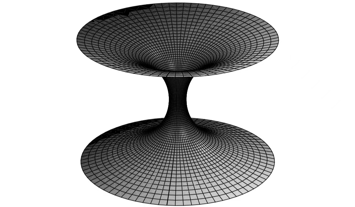
Figure 2. Catenoid

Let $M,M_{1},\cdots,M_{\vartheta}$ be Riemannian manifolds (with boundaries possibly) of the same dimension. Say that $M$ is a connected sum of $M_{1},\cdots,M_{\vartheta}$ (see Fig. 3), if there is a compact subset $K\subset M$ (with nonempty interior) such that $M\setminus K$ is a disjoint union of $\vartheta$ open subsets $E_{1},\cdots,E_{\vartheta},$ where each $E_{j}$ is isomorphic to $M_{j}\setminus K_{j}$ for some compact subset $K_{j}\subset M_{j}.$ When $M,M_{j}^{,}s$ are complex manifolds, the isometries are required to be analytical. We refer to $K$ as the central part of $M$ and refer to $E_{1},\cdots,E_{\vartheta}$ as the ends of $M.$ We also regard $M_{1},\cdots,M_{\vartheta}$ as the ends of $M$ for convenience. By definition, each $E_{j}$ can be identified with $M_{j}\setminus K_{j}.$ For two weighted manifolds $(M,\mu),(M_{j},\mu_{j}),$ the isometry is understood in the sense of weighted manifolds: it maps $\mu$ to $\mu_{j},$ i.e., $\mu,\mu_{j}$ coincide on $E_{j}.$ It is worth mentioning that taking a connected sum is not a uniquely determined operation.

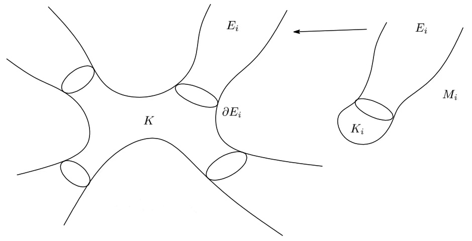
Figure 3. Manifold with ends

For convenience, the connected sum $M=M_{1}\#\cdots\#M_{\vartheta}$ with central part $K$ and ends $E_{1},\cdots,E_{\vartheta}$ is also written as the form

$$M=\left(K;\{M_{j}\}_{j=1}^{\vartheta};\{E_{j}\}_{j=1}^{\vartheta}\right).$$

Let $\partial E_{j}$ be the topological boundary of $E_{j}$ with $j=1,\cdots,\vartheta.$ Write

$$\partial E_{j}=(\partial E_{j}\setminus\delta M)\cup\delta E_{j},$$

where $\partial E_{j}\setminus\delta M$ is called the Dirichlet boundary of $E_{j},$ and $\delta E:=\partial E_{j}\cap\delta M$ is called the Neumann boundary of $E_{j}.$ It is trivial to examine

$$M=K\cup(\cup_{j=1}^{\vartheta}E_{j}),\ \ \ \ \partial K=\cup_{j=1}^{\vartheta}(\partial E_{j}\setminus\delta M).$$

Conversely, for a non-compact manifold $M$ (the compact case can be dealt with similarly), if there is a compact subset $K\subset M$ with smooth boundary such that $M\setminus K$ is a disjoint union of $\vartheta$ connected open subsets $E_{1},\cdots,E_{\vartheta}$ which are not precompact, then we say that $E_{1},\cdots,E_{\vartheta}$ are the ends of $M.$ Consider now the closure $\overline{E}_{j}:=E_{j}\cup\partial E_{j}$ as a manifold with boundary $\partial E_{j}.$ By the definition of connected sums, we have

$$M=\overline{E}_{1}\#\cdots\#\overline{E}_{\vartheta}=\left(K;\{\overline{E}_{j}\}_{j=1}^{\vartheta};\{E_{j}\}_{j=1}^{\vartheta}\right).$$

2.4. Almost Complex Structures of Connected Sums

Let $M=M_{1}\#\cdots\#M_{\vartheta},$ where all $M_{j}^{,}s$ are now almost complex manifolds of the same dimension $m.$ It is aways possible for the existence of an almost complex structure for $m=2,6,$ since every orientable smooth 2-dimensional manifold is almost complex; for a smooth orientable 6-dimensional manifold, where the only obstruction to the existence of an almost complex structure is the third Stiefel-Whitney class $W_{3}$ [41] which is additive under the connected sums. When one of $M_{j}^{,}s$ is non-compact, Albanese-Milivojević [3] proved the existence of an almost complex structure as follows.

Theorem 2.7 ([3], Theorem B).

If one of $M_{j}^{,}s$ is non-compact, then $M$ admits an almost complex structure.

However, it may be impossible if all $M_{j}^{,}s$ are closed. For example, consider the case when $m=4k.$ F. Hirzebruch (see [26], p. 777) showed that the Euler characteristic of $M_{j}$ must satisfy that

$$\chi(M_{j})\equiv(-1)^{k}\tau(M_{j})\ \text{mod}\ 4,$$

where $\tau(M_{j})$ is the signature of $M_{j}$ (see [40]). On the other hand, by

$$\tau(M)=\sum_{j=1}^{\vartheta}\tau(M_{j}),\ \ \ \ \chi(M)=\sum_{j=1}^{\vartheta}\chi(M_{j})-2(\vartheta-1),$$

we deduce that

$$\chi(M)\equiv(-1)^{k}\tau(M)-2(\vartheta-1)\ \text{mod}\ 4.$$

It is therefore

$$\chi(M)\not\equiv(-1)^{k}\tau(M)\ \text{mod}\ 4$$

for an even number $\vartheta,$ i.e., $M$ does not support an almost complex structure for $m=4k$ and $\vartheta=2l.$ But, for which values of $\vartheta$ is $M$ necessarily an almost complex manifold? Some results of existence were obtained in [3, 18, 55, 56]. For example, Albanese-Milivojević [3] showed the following theorem.

Theorem 2.8 ([3], Theorem C).

Assume that all $M_{j}^{,}s$ are closed, then $M$ admits an almost complex structure if one of the following is satisfied$:$

$(a)$ $m=8k+2,$ and $\nu\equiv 1$ mod $(4k)!;$

$(b)$ $m=8k+6,$ and $\nu\equiv 1$ mod $\frac{(4k+2)!}{2}.$

2.5. Heat Kernel on Connected Sums

Let

$$M=\left(K;\{M_{j}\}_{j=1}^{\vartheta};\{E_{j}\}_{j=1}^{\vartheta}\right)$$

be a connected sum, where $(M,\mu),(M_{1},\mu_{1}),\cdots,(M_{\vartheta},\mu_{\vartheta})$ are complete non-compact weighted manifolds. Let $p(t,x,y)$ be the heat kernel of $(M,\mu).$ We recall that $B(x,r)$ is the geodesic ball centered at $x$ with radius $r$ in $M.$ For any $x\in K\cup E_{j}$ with $j=1,\cdots,\vartheta,$ put

$$V_{j}(x,r)=\mu\left(B(x,r)\cap(K\cup E_{j})\right).$$

Fix a reference point $o$ in the interior of $K.$ Set

$$V_{0}(r)=\mathop{\mathrm{min}}_{1\leq j\leq\nu}V_{j}(r)$$

with

$$V_{j}(r)=V_{j}(o,r),\ \ \ \ j=1,\cdots,\vartheta.$$

Again, set for $x\in M$

$$|x|=\sup_{y\in K}d(x,y).$$

Note that $|x|$ is bounded away from 0 due to the compactness of $K.$ Define a positive function $H(x,t)$ on $M\times(0,\infty)$ as follows

$$H(x,t)=\mathop{\mathrm{min}}\left\{1,\ \frac{|x|^{2}}{V_{i_{x}}(|x|)}+\left(\int_{|x|^{2}}^{t}\frac{ds}{V_{i_{x}}(\sqrt{s})}\right)^{+}\right\},$$

where

$$i_{x}=\begin{cases}0,\ \ &x\in K;\\ j,\ \ &x\in E_{j}\ \text{for some}\ j.\end{cases}$$

Evidently, $H(x,t)$ is also bounded away from 0 if $|x|$ is bounded from above. When $V_{i_{x}}(r)$ satisfies

$$\frac{V_{i_{x}}(r_{2})}{V_{i_{x}}(r_{1})}\geq C\left(\frac{r_{2}}{r_{1}}\right)^{2+\epsilon},\ \ \ \ r_{2}>r_{1}\geq 1$$

for some $C,\epsilon>0,$ we obtain

$$H(x,t)\simeq\frac{|x|^{2}}{V_{i_{x}}(|x|)}$$

(see details in the proof of Corollary 4.5, [22]). Let $\gamma:[0,1]\to M$ be a curve with $\gamma(0)=x$ and $\gamma(1)=y.$ Denote by $\|\gamma\|$ the length of $\gamma.$ Set

$$d_{\emptyset}(x,y)=\begin{cases}\inf\big{\{}\|\gamma\|:\gamma\cap K=\emptyset\big{\}},&x,y\in E_{j}\ \text{for some}\ j;\\ \infty,&\text{otherwise}\end{cases}$$

and

$$d_{+}(x,y)=\inf\big{\{}\|\gamma\|:\gamma\cap K\not=\emptyset\big{\}}.$$

It is not hard to verify

(4) $$d(x,y)=\mathop{\mathrm{min}}\big{\{}d_{\emptyset}(x,y),\ d_{+}(x,y)\big{\}}.$$

When $x,y$ belong to the same end, we have

$$d(x,y)\leq d_{\emptyset}(x,y)\leq d(x,y)+C_{K},$$

$$\ \ \ \ |x|+|y|-2{\rm{diam}}(K)\leq d_{+}(x,y)\leq|x|+|y|,$$

where $C_{K}\geq 0$ is a constant depending only on $K.$

Theorem 2.9 ([25], Theorem 4.9).

Let $(M,\mu)$ be a connected sum of complete non-compact weighted manifolds $(M_{1},\mu_{1}),\cdots,(M_{\nu},\mu_{\nu}).$ Assume that $(M,\mu)$ is non-parabolic and each $(M_{j},\mu_{j})$ satisfies $(FK).$ Then, there exist constants $C_{2},c_{2}>0$ such that

$$p(t,x,y) \leq C_{2}\left(\frac{H(x,t)H(y,t)}{V_{0}(\sqrt{t})}+\frac{H(x,t)}{V_{i_{y}}(\sqrt{t})}+\frac{H(y,t)}{V_{i_{x}}(\sqrt{t})}\right)\exp\left(-\frac{d_{+}(x,y)^{2}}{c_{2}t}\right)$$

$$+\frac{C_{2}}{\sqrt{V_{i_{x}}(x,\sqrt{t})V_{i_{y}}(y,\sqrt{t})}}\exp\left(-\frac{d_{\emptyset}(x,y)^{2}}{c_{2}t}\right)$$

holds for all $x,y\in M$ and all $t>0.$

Each term in the upper bound of $p(t,x,y)$ in Theorem 2.9 has a geometric meaning, corresponding to a certain way that a Brownian particle may move from $x$ to $y.$ To start with, the last term estimates the probability of getting from $x$ to $y$ without touching $K.$ The third term (similarly, the second term) estimates the probability that started at $x,$ a Brownian particle hits $K$ before time $t$ and then reaches $y$ in time of order $t.$ Finally, the first term estimates the probability that a Brownian particle hits $K$ before time $t,$ loops from $K$ to $K$ in time of order $t,$ and finally reaches $y$ in time smaller than $t.$

Theorem 2.10 ([25], Theorem 5.10).

Let $(M,\mu)$ be a connected sum of complete non-compact weighted manifolds $(M_{1},\mu_{1}),\cdots,(M_{\vartheta},\mu_{\vartheta}).$ Assume that each $(M_{j},\mu_{j})$ is non-parabolic satisfying $(PH).$ Then, there exist constants $C_{1},c_{1}>0$ such that

$$p(t,x,y) \geq C_{1}\left(\frac{H(x,t)H(y,t)}{V_{0}(\sqrt{t})}+\frac{H(x,t)}{V_{i_{y}}(\sqrt{t})}+\frac{H(y,t)}{V_{i_{x}}(\sqrt{t})}\right)\exp\left(-\frac{d_{+}(x,y)^{2}}{c_{1}t}\right)$$

$$+\frac{C_{1}}{\sqrt{V_{i_{x}}(x,\sqrt{t})V_{i_{y}}(y,\sqrt{t})}}\exp\left(-\frac{d_{\emptyset}(x,y)^{2}}{c_{1}t}\right)$$

holds for all $x,y\in M$ and all $t>0.$

According to Theorem 2.6, we see that $(PH)$ implies $(FK).$ Furthermore, using Proposition 14.1 in [21], we also note that the non-parabolicity of one end $(M_{j},\mu_{j})$ implies the non-parabolicity of $(M,\mu).$ Hence, the upper bound of the heat kernel given in Theorem 2.9 remains valid under the conditions in Theorem 2.10.

3. Setups on Complete Kähler Connected Sums

3.1. Itô Formula

Let $M$ be a complete Riemannian manifold with Laplace-Beltrami operator $\Delta.$ Let $X_{t}$ be the Brownian motion generated by $\Delta/2$ on $M.$ We denote by $\mathbb{P}_{o}$ the law of $X_{t}$ starting from a fixed reference point $o\in M,$ and denote by $\mathbb{E}_{o}$ the expectation of $X_{t}$ with respect to $\mathbb{P}_{o}.$

The famous Itô formula (see [6, 29, 45]) states that

Theorem 3.1 (Itô Formula).

Let $\phi$ be a function of $\mathscr{C}^{2}$-class on $M.$ Then

$$\phi(X_{t})-\phi(o)=\frac{1}{2}\int_{0}^{t}\Delta\phi(X_{s})ds+B\left(\int_{0}^{t}\|\nabla\phi\|^{2}(X_{s})ds\right),\ \ \ \ \mathbb{P}_{o}-a.s.$$

where $B_{t}$ is the standard Brownian motion on $\mathbb{R}.$

Note that Brownian motion is a continuous martingale, thus we have

$$\mathbb{E}_{o}\left[B\left(\int_{0}^{t}\|\nabla\phi\|^{2}(X_{s})ds\right)\right]=B_{0}=0.$$

Hence, it yields from Itô formula that

Corollary 3.2 (Dynkin Formula).

Let $\phi$ be a function of $\mathscr{C}^{2}$-class on $M.$ Then

$$\mathbb{E}_{o}\left[\phi(X_{T})\right]-\phi(o)=\frac{1}{2}\mathbb{E}_{o}\left[\int_{0}^{T}\Delta\phi(X_{t})dt\right]$$

for a finite stopping time $T$ such that each integrand above is integrable.

Dynkin formula plays an important role in the study of Nevanlinna theory on complex manifolds. In the following, we shall give its closest consequence to Nevanlinna theory through the connection between Brownian motion and potential theory. Given an arbitrary bounded domain $\Omega$ (containing $o$) with smooth boundary $\partial\Omega$ in $M.$ Let $g_{\Omega}(x,y)$ denote the Green function of $\Delta/2$ for $\Omega$ with a pole at $o$ satisfying Dirichlet boundary condition, and let $\pi_{\partial\Omega}$ denote the harmonic measure on $\partial\Omega$ with respect to $o.$ Note that

$$d\pi_{\partial\Omega}=\frac{1}{2}\frac{\partial g_{\Omega}(o,x)}{\partial{\vec{\nu}}}d\sigma_{\partial\Omega},$$

where $\partial/\partial\vec{\nu}$ is the inward normal derivative on $\partial\Omega(r),$ $d\sigma_{\partial\Omega}$ is the Riemannian area element of $\partial\Omega(r).$

Historically, the first theorem indicating the connection between Brownian motion and potential theory was obtained by S. Kakutani [32] in 1944. The further relation was investigated by J. Doob [14, 15], G. Hunt [27], A. Knapp [30], N. Privault [45] and Port-Stone [46], etc. In the following, we introduce two classical formulas relating closely to Nevanlinna theory (see [6, 45, 46]).

Let $\phi$ be a continuous function outside a possible polar set of singularities at most on $M.$ The co-area formula reads that

(5) $$\int_{\Omega}g_{\Omega}(o,x)\phi dv=\mathbb{E}_{o}\left[\int_{0}^{\tau_{\Omega}}\phi(X_{t})dt\right],$$

where $dv$ is the Riemannian volume element of $M,$ and $\Delta\phi$ is understood in the sense of distributions. Define the first existing time for $\Omega$

$$\tau_{\Omega}=\inf\big{\{}t>0:X_{t}\not\in\Omega\big{\}},$$

which is a stopping time. We have the probabilistic expression of mean-value integral as follows

(6) $$\int_{\partial\Omega}\phi d\pi_{\partial\Omega}=\mathbb{E}_{o}\left[\phi(X_{\tau_{\Omega}})\right].$$

Set $T=\tau_{\Omega}$ and apply (5) with (6) in Corollary 3.2, the Dynkin formula also holds in the viewpoint of distributions since the possible set of singularities of $\phi$ is polar. Hence, we have:

Corollary 3.3 (Jensen-Dynkin Formula).

Let $\phi$ be a $\mathscr{C}^{2}$-function outside a possible polar set of singularities at most on $M.$ Assume that $\phi(o)\not=\infty.$ Then

$$\int_{\partial\Omega}\phi d\pi_{\partial\Omega}-\phi(o)=\frac{1}{2}\int_{\Omega}g_{\Omega}(o,x)\Delta\phi dv,$$

where $\Delta\phi$ is understood in the sense of distributions.

When $M=\mathbb{C}^{m},$ the Green function and harmonic measure for balls have explicit expressions. By a direct computation, we will see that Green-Jensen formula (see [42, 47]) follows from Jensen-Dynkin formula.

3.2. Complete Kähler Connected Sums

We first give the notion of Kähler connected sums as follows.

Definition 3.4.

Let $M$ be a Kähler manifold. We say that $M$ is a Kähler connected sum with $\vartheta$ ends, if there exist $\vartheta$ Kähler manifolds $M_{1},\cdots,M_{\vartheta}$ such that $M=M_{1}\#\cdots\#M_{\vartheta}.$ In addition, we say that $M$ is complete if all $M_{j}^{,}s$ are complete.

Let

$$M=\left(K;\{M_{j}\}_{j=1}^{\vartheta};\{E_{j}\}_{j=1}^{\vartheta}\right)$$

be a complete Kähler connected sum with $\vartheta$ non-parabolic ends (by which we mean that all $M_{j}^{,}s$ are non-parabolic), where all $M_{j}^{,}s$ are assumed to be non-compact. As noted in Section 2.5, $M$ is also non-parabolic.

Let $\Delta$ denote the Laplace-Beltrami operator on $M.$ We consider the heat kernel $p(t,x,y)$ of $M,$ which is the minimal positive fundamental solution to the heat equation

$$\left(\Delta-\frac{\partial}{\partial t}\right)u(t,x)=0.$$

We first review some notations. Fix a fixed reference point in the interior of $K.$ We denote by $B(r)$ the geodesic ball centered at $o$ with radius $r$ in $M,$ and by $d(x,y)$ the Riemannian distance between $x,y\in M.$ Set

(7) $$V_{\rm min}(r)=\mathop{\mathrm{min}}_{1\leq j\leq\vartheta}V_{j}(r),\ \ \ \ V_{\rm max}(r)=\max_{1\leq j\leq\vartheta}V_{j}(r)$$

with

$$V_{j}(r)={\rm{Vol}}\left(B(r)\cap(K\cup E_{j})\right),\ \ \ \ j=1,\cdots,\vartheta.$$

Put

$$\rho(x)=d(o,x),\ \ \ \ |x|=\sup_{y\in K}d(x,y).$$

Again, define the function $H(x,t)$ on $M\times(0,\infty)$ as follows

(8) $$H(x,t)=\mathop{\mathrm{min}}\left\{1,\ \frac{|x|^{2}}{V_{i_{x}}(|x|)}+\left(\int_{|x|^{2}}^{t}\frac{ds}{V_{i_{x}}(\sqrt{s})}\right)^{+}\right\},$$

where

$$i_{x}=\begin{cases}j,\ &x\in E_{j}\ \text{for some}\ j;\\ 0,\ &x\in K.\end{cases}$$

We give two-sided bounds of $p(t,o,x)$ using Theorems 2.9 and 2.10. Since $o\in K,$ then it follows from (4) and definitions of $d_{\emptyset}(x,y)$ and $d_{+}(x,y)$ that

(9) $$d_{\emptyset}(o,x)=\infty,\ \ \ \ d_{+}(o,x)=\rho(x).$$

Notice that $K\subset M$ is a compact subset with nonempty interior, we obtain $0<|o|<\infty.$ From $i_{o}=0$ and (8), it is not difficult to derive

(10) $$0<\gamma_{0}:=\mathop{\mathrm{min}}\left\{1,\ \frac{|o|^{2}}{V_{\rm max}(|o|)}\right\}\leq H(o,t)\leq 1,\ \ \ \ 0<H(x,t)\leq 1.$$

Set

$$W(x,t)=\frac{H(o,t)H(x,t)}{V_{\mathop{\mathrm{min}}}(\sqrt{t})}+\frac{H(o,t)}{V_{i_{x}}(\sqrt{t})}+\frac{H(x,t)}{V_{i_{o}}(\sqrt{t})}.$$

It follows from (7) and (10) that

(11) $$\frac{\gamma_{0}}{V_{\rm max}(\sqrt{t})}\leq W(x,t)\leq\frac{3}{V_{\rm min}(\sqrt{t})}.$$

Note that $(PH)$ implies $(FH)$ and the non-parabolicity of any $M_{j}$ implies the non-parabolicity of $M.$ Combining (9) with (11) and using Theorems 2.9 and 2.10, we obtain:

Corollary 3.5.

Let $M=(K;\{M_{j}\}_{j=1}^{\vartheta};\{E_{j}\}_{j=1}^{\vartheta})$ be a complete Kähler connected sum with $\vartheta$ non-parabolic ends, where all $M_{j}^{,}s$ are non-compact. Assume that all $M_{j}^{,}s$ satisfy $(PH).$ Then, there exist constants $A,B,a,b>0$ such that

$$\frac{A}{V_{\rm max}(\sqrt{t})}\exp\left(-\frac{\rho(x)^{2}}{at}\right)\leq p(t,o,x)\leq\frac{B}{V_{\rm min}(\sqrt{t})}\exp\left(-\frac{\rho(x)^{2}}{bt}\right)$$

holds for all $x\in M$ and all $t>0.$

3.3. Nevanlinna’s Functions via Heat Kernel

Let

$$M=M_{1}\#\cdots\#M_{\vartheta}$$

be a complete Kähler connected sum with $\vartheta$ non-parabolic ends, in which all $M_{j}^{,}s$ are non-compact satisfying $(PH)$ in Property 2.5, of complex dimension $m.$ Assume the Kähler form of $M$ associated to Kähler metric $g=(g_{i\bar{j}})$

$$\alpha=\frac{\sqrt{-1}}{\pi}\sum_{i,j=1}^{m}g_{i\bar{j}}dz_{i}\wedge d\bar{z}_{j}$$

in a holomorphic local coordinate $(z_{1},\cdots,z_{m}).$ We adopt the same notations as defined in Section 3.2. By Corollary 3.5, there exist constants $A,B,a,b>0$ such that

(12) $$\frac{A}{V_{\rm max}(\sqrt{t})}\exp\left(-\frac{\rho(x)^{2}}{at}\right)\leq p(t,o,x)\leq\frac{B}{V_{\rm min}(\sqrt{t})}\exp\left(-\frac{\rho(x)^{2}}{bt}\right)$$

holds for all $x\in M$ and all $t>0.$ Since $M$ is non-parabolic, then the infinite integral

$$G(o,x):=2\int_{0}^{\infty}p(t,o,x)dt$$

is convergent for $x\not=o,$ which is the minimal positive Green function of $\Delta/2$ for $M$ with a pole at $o.$ The non-parabolicity of all $M_{j}^{,}s$ also imply that

$$\int_{0}^{\infty}\frac{e^{-\frac{\rho(x)^{2}}{at}}}{V_{\rm max}(\sqrt{t})}dt,\ \ \ \ \int_{0}^{\infty}\frac{e^{-\frac{\rho(x)^{2}}{bt}}}{V_{\rm min}(\sqrt{t})}dt$$

are convergent for $x\not=o$ due to Theorem 2.4. Moreover, each of them tends to $0$ as $x\to\infty$ and tends to $\infty$ as $x\to o.$ It yields from Corollary 3.5 that

(13) $$2A\int_{0}^{\infty}\frac{e^{-\frac{\rho(x)^{2}}{at}}}{V_{\rm max}(\sqrt{t})}dt\leq G(o,x)\leq 2B\int_{0}^{\infty}\frac{e^{-\frac{\rho(x)^{2}}{bt}}}{V_{\rm min}(\sqrt{t})}dt$$

for all $x\in M.$

In order to define Nevanlinna’s functions, it is needed to construct a family of suitable precompact domains $\Delta(r)$ containing $o,$ being able to exhaust $M.$ One workable way is based on the heat kernel $p(t,o,x),$ because it is effective for estimate of Green function for $\Delta(r)$ (with a pole at $o$ satisfying Dirichelet boundary condition). For $r>0,$ define

$$\Delta(r)=\left\{x\in M:\ G(o,x)>2A\int_{0}^{\infty}\frac{e^{-\frac{r^{2}}{at}}}{V_{\rm max}(\sqrt{t})}dt\right\}.$$

By

$$\int_{0}^{\infty}\frac{e^{-\frac{r^{2}}{At}}}{V_{\rm max}(\sqrt{t})}dt\searrow 0,\ \ \ \ r\to\infty$$

with

$$\lim_{x\to o}G(o,x)=\infty,\ \ \ \ \lim_{x\to\infty}G(o,x)=0,$$

we see that $\Delta(r)$ is a precompact domain containing $o$ in $M$ such that

$$\ \ \ \lim_{r\to 0}\Delta(r)\to\emptyset,\ \ \ \ \lim_{r\to\infty}\Delta(r)=M.$$

Moreover, the family $\{\Delta(r)\}_{r>0}$ exhausts $M,$ for any sequence $\{r_{n}\}_{n=1}^{\infty}$ with $0<r_{1}<r_{2}<\cdots\to\infty,$ we have

$$\bigcup_{n=1}^{\infty}\Delta(r_{n})=M,\ \ \ \ \emptyset\not=\Delta(r_{1})\subset\overline{\Delta(r_{1})}\subset\Delta(r_{2})\subset\overline{\Delta(r_{2})}\subset\cdots$$

Whence, the boundary of $\Delta(r)$ can be formulated as

$$\partial\Delta(r)=\left\{x\in M:\ G(o,x)=2A\int_{0}^{\infty}\frac{e^{-\frac{r^{2}}{at}}}{V_{\rm max}(\sqrt{t})}dt\right\}.\$$

By Sard’s theorem, each connected component of $\partial\Delta(r)$ is a submanifold of $M$ for almost all $r>0.$

Define

$$g_{r}(o,x)=G(o,x)-2A\int_{0}^{\infty}\frac{e^{-\frac{r^{2}}{at}}}{V_{\rm max}(\sqrt{t})}dt.$$

Then, we see that $g_{r}(o,x)$ defines the Green function of $\Delta/2$ for $\Delta(r)$ with a pole at $o$ satisfying Dirichelet boundary condition. Let $\pi_{r}$ be the harmonic measure on $\partial\Delta(r)$ with respect to $o,$ i.e.,

$$d\pi_{r}=\frac{1}{2}\frac{\partial g_{r}(o,x)}{\partial{\vec{\nu}}}d\sigma_{r},$$

where $\partial/\partial\vec{\nu}$ is the inward normal derivative on $\partial\Delta(r),$ $d\sigma_{r}$ is the Riemannian area element of $\partial\Delta(r).$

Now, we define the Nevanlinna’s functions. Let $X$ be a complex projective manifold, over which we can put a Hermitian holomorphic line bundle $(L,h)$ with Chern form $c_{1}(L,h):=-dd^{c}\log h,$ where

$$d=\partial+\overline{\partial},\ \ \ \ d^{c}=\frac{\sqrt{-1}}{4\pi}(\overline{\partial}-\partial)$$

so that

$$dd^{c}=\frac{\sqrt{-1}}{2\pi}\partial\overline{\partial}.$$

Let $f:M\to X$ be a meromorphic mapping. The characteristic function of $f$ with respect to $L$ is defined by

$$T_{f}(r,L) = \frac{\pi^{m}}{(m-1)!}\int_{\Delta(r)}g_{r}(o,x)f^{*}c_{1}(L,h)\wedge\alpha^{m-1}$$

$$= -\frac{1}{4}\int_{\Delta(r)}g_{r}(o,x)\Delta\log(h\circ f)dv,$$

where $dv$ is the Riemannian volume element of $M.$

Let $s_{D}$ be the canonical section associated to $D\in|L|,$ namely, $s_{D}$ is the holomorphic section of $L$ over $X$ with zero divisor $D.$ The proximity function of $f$ with respect to $D$ is defined by

$$m_{f}(r,D)=\int_{\partial\Delta(r)}\log\frac{1}{\|s_{D}\circ f\|}d\pi_{r}.$$

Meanwhile, we define the counting function and the simple counting function of $f$ with respect to $D$ respectively by

$$N_{f}(r,D) = \frac{\pi^{m}}{(m-1)!}\int_{f^{*}D\cap\Delta(r)}g_{r}(o,x)\alpha^{m-1},$$

$$\overline{N}_{f}(r,D) = \frac{\pi^{m}}{(m-1)!}\int_{f^{-1}(D)\cap\Delta(r)}g_{r}(o,x)\alpha^{m-1}.$$

The characteristic function of $\mathscr{R}=-dd^{c}\log\det(g_{i\bar{j}})$ is defined by

$$T(r,\mathscr{R}) = \frac{\pi^{m}}{(m-1)!}\int_{\Delta(r)}g_{r}(o,x)\mathscr{R}\wedge\alpha^{m-1}$$

$$= -\frac{1}{4}\int_{\Delta(r)}g_{r}(o,x)\Delta\log\det(g_{i\bar{j}})dv.$$

When $M=\mathbb{C}^{m}$

(14) $$p(t,\textbf{0},z)=\frac{1}{(4\pi t)^{m}}e^{-\frac{\|z\|^{2}}{4t}}.$$

We consider the non-parabolic case (i.e., $m\geq 2$). By definition

$$G(\textbf{0},z)=2\int_{0}^{\infty}\frac{e^{-\frac{\|z\|^{2}}{4t}}}{(4\pi t)^{m}}dt,$$

which gives that

$$\Delta(r) = \left\{x\in\mathbb{C}^{m}:\ G(\textbf{0},z)>2\int_{0}^{\infty}\frac{e^{-\frac{r^{2}}{4t}}}{(4\pi t)^{m}}dt\right\}$$

$$= \big{\{}z\in\mathbb{C}^{m}:\|z\|<r\big{\}}:=\mathbb{B}(r)$$

and

$$g_{r}(\textbf{0},z) = 2\int_{0}^{\infty}\frac{e^{-\frac{\|z\|^{2}}{4t}}}{(4\pi t)^{m}}dt-2\int_{0}^{\infty}\frac{e^{-\frac{r^{2}}{4t}}}{(4\pi t)^{m}}dt$$

$$= \frac{\|z\|^{2-2m}-r^{2-2m}}{(m-1)\omega_{2m-1}},$$

where $\omega_{2m-1}$ is the area of the unit sphere in $\mathbb{C}^{m}.$ It further derives

$$d\pi_{r}(z)=d^{c}\log\|z\|^{2}\wedge\left(dd^{c}\log\|z\|^{2}\right)^{m-1}.$$

By integration-by-parts formula, we shall see that our Nevanlinna’s functions agree with the classical ones. Notice the connection between potential theory and Brownian motion, Nevanlinna’s functions have alternative probabilistic expressions as follows.

Let $\mathbb{P}_{o}$ denote the law of $X_{t}$ starting from $o,$ whose associated expectation is denoted by $\mathbb{E}_{o}.$ The first existing time for $\Delta(r)$ is defined by

$$\tau_{r}=\inf\big{\{}t>0:X_{t}\not\in\Delta(r)\big{\}}.$$

By co-area formula (see (5)), we can deduce that

$$T_{f}(r,L) =-\frac{1}{4}\mathbb{E}_{o}\left[\int_{0}^{\tau_{r}}\Delta\log(h\circ f(X_{t}))dt\right],$$

$$T(r,\mathscr{R}) =-\frac{1}{4}\mathbb{E}_{o}\left[\int_{0}^{\tau_{r}}\Delta\log\det(g_{i\bar{j}}(X_{t}))dt\right].$$

At the same time, (6) yields that

$$m_{f}(r,D)=\mathbb{E}_{o}\left[\log\frac{1}{\|s_{D}\circ f(X_{\tau_{r}})\|}\right].$$

Moreover, we have ((see [1, 2, 9, 16])

$$N_{f}(r,D)=\lim_{\lambda\rightarrow\infty}\lambda\mathbb{P}_{o}\left(\sup_{0\leq t\leq\tau_{r}}\log\frac{1}{\|s_{D}\circ f(X_{t})\|}>\lambda\right).$$

However, there exists no such an analytic expression for $\overline{N}_{f}(r,D)$ in general. Using Poincaré-Lelong formula (see [12, 42, 47]) and Jensen-Dynkin formula (see Corollary 3.3), it is immediate to derive the following first main theorem.

Theorem 3.6 ([16]).

Assume that $f(o)\not\in{\rm{Supp}}D.$ Then

$$T_{f}(r,L)+\log\frac{1}{\|s_{D}\circ f(o)\|}=m_{f}(r,D)+N_{f}(r,D).$$

3.4. Ahlfors-Shimizu Form of $T_{f}(r,L)$

In order to better understand the characteristic function $T_{f}(r,L),$ we want to describe how similar $T_{f}(r,L)$ is to the classical characteristic function. We shall prove that $T_{f}(r,L)$ has an alternative form very like Ahlfors-Shimizu’s characteristic function.

Lemma 3.7.

For $0<t\leq r,$ we have

$$g_{r}(o,x)=2A\int_{0}^{\infty}\frac{e^{-\frac{t^{2}}{as}}-e^{-\frac{r^{2}}{as}}}{V_{\max}(\sqrt{s})}ds$$

for all $x\in\partial\Delta(t).$

Proof.

The definition of $\partial\Delta(t)$ gives that

$$g_{t}(o,x)=G(o,x)-2A\int_{0}^{\infty}\frac{e^{-\frac{t^{2}}{as}}}{V_{\rm max}(\sqrt{s})}ds=0$$

for $x\in\partial\Delta(t).$ It is therefore

$$g_{r}(o,x) = G(o,x)-2A\int_{0}^{\infty}\frac{e^{-\frac{r^{2}}{at}}}{V_{\rm max}(\sqrt{t})}dt$$

$$= G(o,x)-2A\int_{0}^{\infty}\frac{e^{-\frac{t^{2}}{as}}}{V_{\rm max}(\sqrt{s})}ds+2A\int_{0}^{\infty}\frac{e^{-\frac{t^{2}}{as}}}{V_{\rm max}(\sqrt{s})}ds$$

$$-2A\int_{0}^{\infty}\frac{e^{-\frac{r^{2}}{as}}}{V_{\rm max}(\sqrt{s})}ds$$

$$= 2A\int_{0}^{\infty}\frac{e^{-\frac{t^{2}}{as}}-e^{-\frac{r^{2}}{as}}}{V_{\max}(\sqrt{s})}ds$$

for $x\in\partial\Delta(t).$ ∎

Lemma 3.7 is useful for the establishment of calculus lemma in Section 4. Here, we give its another application.

Theorem 3.8.

$T_{f}(r,L)$ has the Ahlfors-Shimizu form

$$T_{f}(r,L) = \frac{4A\pi^{m}}{(m-1)!a}\int_{0}^{r}t\int_{0}^{\infty}\frac{e^{-\frac{t^{2}}{as}}}{V_{\max}(\sqrt{s})}\frac{ds}{s}dt\int_{\Delta(t)}f^{*}c_{1}(L,h)\wedge\alpha^{m-1}.$$

Proof.

By integration-by-parts formula and Lemma 3.7, we have

$$\frac{4A\pi^{m}}{(m-1)!a}\int_{0}^{r}t\int_{0}^{\infty}\frac{e^{-\frac{t^{2}}{as}}}{V_{\max}(\sqrt{s})}\frac{ds}{s}dt\int_{\Delta(t)}f^{*}c_{1}(L,h)\wedge\alpha^{m-1}$$

$$= -\frac{A}{a}\int_{0}^{r}t\int_{0}^{\infty}\frac{e^{-\frac{t^{2}}{as}}}{V_{\max}(\sqrt{s})}\frac{ds}{s}dt\int_{\Delta(t)}\Delta\log(h\circ f)dv$$

$$= \frac{A}{2}\int_{0}^{r}d\int_{0}^{\infty}\frac{e^{-\frac{t^{2}}{as}}-e^{-\frac{r^{2}}{as}}}{V_{\max}(\sqrt{s})}ds\int_{\Delta(t)}\Delta\log(h\circ f)dv$$

$$= \frac{A}{2}\left[\int_{0}^{\infty}\frac{e^{-\frac{t^{2}}{as}}-e^{-\frac{r^{2}}{as}}}{V_{\max}(\sqrt{s})}ds\int_{\Delta(t)}\Delta\log(h\circ f)dv\right]_{t=0}^{r}$$

$$-\frac{A}{2}\int_{0}^{r}\int_{0}^{\infty}\frac{e^{-\frac{t^{2}}{as}}-e^{-\frac{r^{2}}{as}}}{V_{\max}(\sqrt{s})}dsd\int_{\Delta(t)}\Delta\log(h\circ f)dv$$

$$= -\frac{A}{2}\int_{0}^{r}dt\int_{0}^{\infty}\frac{e^{-\frac{t^{2}}{as}}-e^{-\frac{r^{2}}{as}}}{V_{\max}(\sqrt{s})}ds\int_{\partial\Delta(t)}\Delta\log(h\circ f)d\sigma_{t}$$

$$= -\frac{A}{2}\int_{0}^{r}dt\int_{\partial\Delta(t)}\int_{0}^{\infty}\frac{e^{-\frac{t^{2}}{as}}-e^{-\frac{r^{2}}{as}}}{V_{\max}(\sqrt{s})}ds\Delta\log(h\circ f)d\sigma_{t}.$$

$$= -\frac{1}{4}\int_{0}^{r}dt\int_{\partial\Delta(t)}g_{r}(o,x)\Delta\log(h\circ f)d\sigma_{t}$$

$$= -\frac{1}{4}\int_{\Delta(r)}g_{r}(o,x)\Delta\log(h\circ f)dv$$

$$= T_{f}(r,L).$$

This completes the proof. ∎

Locally, write $s_{D}=\tilde{s}_{D}e,$ where $e$ is a holomorphic local frame of $L.$ Due to Poincaré-Lelong formula, we have

$$\left[D\right]=dd^{c}\left[\log|\tilde{s}_{D}\circ f|^{2}\right]$$

in the sense of currents. Hence, by means of the similar argument as in the proof of Lemma 3.7, we can also obtain

$$N_{f}(r,D) = \frac{4A\pi^{m}}{(m-1)!a}\int_{0}^{r}t\int_{0}^{\infty}\frac{e^{-\frac{t^{2}}{as}}}{V_{\max}(\sqrt{s})}\frac{ds}{s}dt\int_{f^{*}D\cap\Delta(t)}\alpha^{m-1},$$

$$\overline{N}_{f}(r,D) = \frac{4A\pi^{m}}{(m-1)!a}\int_{0}^{r}t\int_{0}^{\infty}\frac{e^{-\frac{t^{2}}{as}}}{V_{\max}(\sqrt{s})}\frac{ds}{s}dt\int_{f^{-1}(D)\cap\Delta(t)}\alpha^{m-1}.$$

To see it more clearly, we consider $M=\mathbb{C}^{m}$ ($m\geq 2$) as an example. Due to (14) and (3.3), we obtain

$$V_{\max}(\sqrt{t})=\frac{\pi^{m}}{m!}t^{m},\ \ \ \ a=4,\ \ \ \ A=\frac{1}{4^{m}m!},$$

which yields that

$$\frac{4A\pi^{m}}{(m-1)!a}\int_{0}^{\infty}\frac{e^{-\frac{t^{2}}{as}}}{V_{\max}(\sqrt{s})}\frac{ds}{s}=\frac{1}{4^{m}(m-1)!}\int_{0}^{\infty}e^{-\frac{t^{2}}{4s}}\frac{ds}{s^{m+1}}=\frac{1}{t^{2m}}.$$

By this with Theorem 3.8, we are led to

$$T_{f}(r,L) = \int_{0}^{r}\frac{dt}{t^{2m-1}}\int_{\mathbb{B}(t)}f^{*}c_{1}(L,h)\wedge\alpha^{m-1},$$

which is just the Ahlfors-Shimizu’s characteristic function.

4. Two Key Lemmas

The main purpose in this section is to establish two key lemmas: calculus lemma and logarithmic derivative lemma. Recall that

$$M=M_{1}\#\cdots\#M_{\vartheta}$$

is a complete Kähler connected sum with $\vartheta$ non-parabolic ends, in which all $M_{j}^{,}s$ are non-compact satisfying $(PH)$ in Property 2.5.

4.1. Calculus Lemma

Lemma 4.1.

For any $\epsilon>0,$ there exists sufficiently large $r_{\epsilon}>0$ such that

$$d\pi_{r}(x)\leq\left(\frac{2B}{b}+\epsilon\right)\rho(x)\int_{0}^{\infty}\frac{e^{-\frac{\rho(x)^{2}}{bt}}}{V_{\rm min}(\sqrt{t})}\frac{dt}{t}\cdot d\sigma_{r}(x)$$

holds for all $x\in\partial\Delta(r)$ and all $r>r_{\epsilon},$ where $d\sigma_{r}$ is the Riemannian area element of $\partial\Delta(r).$

Proof.

From (13), we have

(16) $$G(o,x)\leq 2B\int_{0}^{\infty}\frac{e^{-\frac{\rho(x)^{2}}{bt}}}{V_{\rm min}(\sqrt{t})}dt$$

for $x\in M.$ Since

$$\lim_{x\to\infty}G(o,x)=0,\ \ \ \ \lim_{x\to\infty}\int_{0}^{\infty}\frac{e^{-\frac{\rho(x)^{2}}{bt}}}{V_{\rm min}(\sqrt{t})}dt=0,$$

then we can use the (generalized) L’Hôspital’s rule. It follows from (16) and L’Hôspital’s rule that

$$\limsup_{r\to\infty}\frac{\partial g_{r}(o,x)/\partial\vec{\nu}}{\partial\displaystyle\int_{0}^{\infty}\frac{e^{-\frac{\rho(x)^{2}}{bt}}}{V_{\rm min}(\sqrt{t})}dt\bigg{/}\partial\vec{\nu}}$$

$$= \limsup_{r\to\infty}\frac{\partial G(o,x)/\partial\vec{\nu}}{\partial\displaystyle\int_{0}^{\infty}\frac{e^{-\frac{\rho(x)^{2}}{bt}}}{V_{\rm min}(\sqrt{t})}dt\bigg{/}\partial\vec{\nu}}$$

$$= \limsup_{r\to\infty}\frac{\|\nabla G(o,x)\|}{\partial\displaystyle\int_{0}^{\infty}\frac{e^{-\frac{\rho(x)^{2}}{bt}}}{V_{\rm min}(\sqrt{t})}dt\bigg{/}\partial\vec{\nu}}$$

$$\leq 2B$$

for $x\in\partial\Delta(r),$ where $\partial/\partial\vec{\nu}$ denotes the inward derivative on $\partial\Delta(r).$ A direct computation leads to

$$\frac{\partial\displaystyle\int_{0}^{\infty}\frac{e^{-\frac{\rho(x)^{2}}{bt}}}{V_{\rm min}(\sqrt{t})}dt}{\partial\vec{\nu}} = \frac{\partial\displaystyle\int_{0}^{\infty}\frac{e^{-\frac{\rho(x)^{2}}{bt}}}{V_{\rm min}(\sqrt{t})}dt}{\partial\rho(x)}\cdot\frac{\partial\rho(x)}{\partial\vec{\nu}}$$

$$= \int_{0}^{\infty}\frac{\partial e^{-\frac{\rho(x)^{2}}{bt}}}{\partial\rho(x)}\frac{dt}{V_{\rm min}(\sqrt{t})}\cdot\frac{\partial\rho(x)}{\partial\vec{\nu}}$$

$$= \frac{2\rho(x)}{b}\int_{0}^{\infty}\frac{e^{-\frac{\rho(x)^{2}}{bt}}}{V_{\rm min}(\sqrt{t})}\frac{dt}{t}\cdot\left(-\frac{\partial\rho(x)}{\partial\vec{\nu}}\right)$$

$$\leq \frac{2\rho(x)}{b}\int_{0}^{\infty}\frac{e^{-\frac{\rho(x)^{2}}{bt}}}{V_{\rm min}(\sqrt{t})}\frac{dt}{t}$$

for $x\in\partial\Delta(r)\setminus Cut(o),$ where $Cut(o)$ is the cut locus of $o.$ Combining the above to conclude that

$$\limsup_{r\to\infty}\frac{\frac{\partial g_{r}(o,x)}{\partial\vec{\nu}}}{\rho(x)\displaystyle\int_{0}^{\infty}\frac{e^{-\frac{\rho(x)^{2}}{Bt}}}{V_{\rm min}(\sqrt{t})}\frac{dt}{t}}\leq\frac{4B}{b}$$

for $x\in\partial\Delta(r)\setminus Cut(o).$ Since $\partial\Delta(r)$ is a compact set for $r>0,$ then for any $\epsilon>0,$ there exists sufficiently large $r_{\epsilon}>0$ such that

(17) $$\frac{\partial g_{r}(o,x)}{\partial\vec{\nu}}\leq\left(\frac{4B}{b}+\epsilon\right)\rho(x)\int_{0}^{\infty}\frac{e^{-\frac{\rho(x)^{2}}{Bt}}}{V_{\rm min}(\sqrt{t})}\frac{dt}{t}$$

holds for all $x\in\partial\Delta(r)\setminus Cut(o)$ with $r>r_{\epsilon}.$ Notice that $Cut(o)$ is a closed set of Riemannian measure 0, using the continuity of $\|\nabla G(o,x)\|$ on $M\setminus\{o\},$ we deduce that $(\ref{m4})$ holds on $Cut(o)$ with $r>r_{\epsilon}.$ Using the definition of $d\pi_{r}$ again, then we prove the lemma. ∎

Lemma 4.2 (Borel’s Lemma).

Let $u\geq 0$ be a non-decreasing function on $(r_{0},\infty)$ with $r_{0}\geq 0.$ Then for any $\delta>0,$ there exists a subset $E_{\delta}\subset(r_{0},\infty)$ of finite Lebesgue measure such that such that

$$u^{\prime}(r)\leq u(r)^{1+\delta}$$

holds for all $r>r_{0}$ outside $E_{\delta}.$

Proof.

The conclusion is clearly true for $u\equiv 0.$ Next, we assume that $u\not\equiv 0.$ Since $u\geq 0$ is a non-decreasing function, then there exists a number $r_{1}>r_{0}$ such that $u(r_{1})>0.$ The non-decreasing property of $u$ implies that the limit $\eta:=\lim_{r\to\infty}u(r)$ exists ($\eta=\infty$ is allowed). If $\eta=\infty,$ then $\eta^{-1}=0.$ Set

$$E_{\delta}=\left\{r\in(r_{0},\infty):u^{\prime}(r)>u(r)^{1+\delta}\right\}.$$

Since $u$ is a non-decreasing function on $(r_{0},\infty),$ then $u^{\prime}(r)$ exists for almost all $r\in(r_{0},\infty).$ It is therefore

$$m(E_{\delta}) = \int_{E_{\delta}}dr$$

$$\leq \int_{r_{0}}^{r_{1}}dr+\int_{r_{1}}^{\infty}\frac{u^{\prime}(r)}{u(r)^{1+\delta}}dr$$

$$= \frac{1}{\delta u(r_{1})^{\delta}}-\frac{1}{\delta\eta^{\delta}}+r_{1}-r_{0}$$

$$< \infty.$$

This completes the proof. ∎

Theorem 4.3 (Calculus Lemma).

Let $k\geq 0$ be a locally integrable function on $M.$ Assume that $k$ is locally bounded at $o.$ Then there is a constant $C>0$ and for any $\delta>0,$ there exists a set $E_{\delta}\subset(0,\infty)$ of finite Lebesgue measure such that

$$\int_{\partial\Delta(r)}kd\pi_{r}\leq C\Xi(r)\left(r\int_{0}^{\infty}\frac{e^{-\frac{r^{2}}{at}}}{V_{\max}(\sqrt{t})}\frac{dt}{t}\right)^{-\delta}\left(\int_{\Delta(r)}g_{r}(o,x)kdv\right)^{(1+\delta)^{2}}$$

holds for all $r>0$ outside $E_{\delta},$ where $\Xi$ is defined by $(\ref{XI}).$

Proof.

Lemma 3.7 yields that

$$\Lambda(r) := \int_{\Delta(r)}g_{r}(o,x)kdv$$

$$= \int_{0}^{r}dt\int_{\partial\Delta(t)}g_{r}(o,x)kd\sigma_{t}$$

$$= 2A\int_{0}^{r}\left(\int_{0}^{\infty}\frac{e^{-\frac{t^{2}}{as}}-e^{-\frac{r^{2}}{as}}}{V_{\max}(\sqrt{s})}ds\right)dt\int_{\partial\Delta(t)}kd\sigma_{t}.$$

Differentiating $\Lambda,$ we obtain

$$\Lambda^{\prime}(r)=\frac{d\Lambda(r)}{dr}=\frac{4Ar}{a}\int_{0}^{\infty}\frac{e^{-\frac{r^{2}}{at}}}{V_{\max}(\sqrt{t})}\frac{dt}{t}\int_{0}^{r}dt\int_{\partial\Delta(t)}kd\sigma_{t}.$$

In further

$$\frac{d}{dr}\left(\frac{a\Lambda^{\prime}(r)}{4Ar\displaystyle\int_{0}^{\infty}\frac{e^{-\frac{r^{2}}{at}}}{V_{\max}(\sqrt{t})}\frac{dt}{t}}\right)=\int_{\partial\Delta(r)}kd\sigma_{r}.$$

Take a small $\delta$ with $0<\delta<1.$ Applying Borel’s lemma to the left hand side on the above equality twice, then there exists a subset $F_{\delta}\subset(0,\infty)$ of finite Lebesgue measure such that

$$\int_{\partial\Delta(r)}kd\sigma_{r}$$

$$\leq \left(\frac{a}{4Ar}\right)^{1+\delta}\left(\int_{0}^{\infty}\frac{e^{-\frac{r^{2}}{at}}}{V_{\max}(\sqrt{t})}\frac{dt}{t}\right)^{-(1+\delta)}\Lambda(r)^{(1+\delta)^{2}}$$

$$= \left(\frac{a}{4Ar}\right)^{1+\delta}\left(\int_{0}^{\infty}\frac{e^{-\frac{r^{2}}{at}}}{V_{\max}(\sqrt{t})}\frac{dt}{t}\right)^{-(1+\delta)}\left(\int_{\Delta(r)}g_{r}(o,x)kdv\right)^{(1+\delta)^{2}}$$

holds for all $r>0$ outside $F_{\delta}.$ In the meanwhile, Lemma 4.1 gives that there exists sufficiently large $r_{0}>0$ such that

(19) $$d\pi_{r}\leq\left(\frac{2B}{b}+\delta\right)\sup_{x\in\partial\Delta(r)}\int_{0}^{\infty}\frac{\rho(x)e^{-\frac{\rho(x)^{2}}{Bt}}}{V_{\rm min}(\sqrt{t})}\frac{dt}{t}\cdot d\sigma_{r}$$

holds for all $r>r_{0}.$ Set

$$C=\sup_{0<\delta<1}\left(\frac{2B}{b}+\delta\right)\left(\frac{a}{4A}\right)^{1+\delta}.$$

Substituting (19) into (4.1), we conclude that

(20) $$\int_{\partial\Delta(r)}kd\pi_{r} \leq C\sup_{x\in\partial\Delta(r)}\frac{\rho(x)\displaystyle\int_{0}^{\infty}\frac{e^{-\frac{\rho(x)^{2}}{Bt}}}{V_{\rm min}(\sqrt{t})}\frac{dt}{t}}{r\displaystyle\int_{0}^{\infty}\frac{e^{-\frac{r^{2}}{At}}}{V_{\max}(\sqrt{t})}\frac{dt}{t}}\left(r\int_{0}^{\infty}\frac{e^{-\frac{r^{2}}{At}}}{V_{\max}(\sqrt{t})}\frac{dt}{t}\right)^{-\delta}$$

$$\cdot\left(\int_{\Delta(r)}g_{r}(o,x)kdv\right)^{(1+\delta)^{2}}$$

$$= C\Xi(r)\left(r\int_{0}^{\infty}\frac{e^{-\frac{r^{2}}{At}}}{V_{\max}(\sqrt{t})}\frac{dt}{t}\right)^{-\delta}\left(\int_{\Delta(r)}g_{r}(o,x)kdv\right)^{(1+\delta)^{2}}$$

for $r>0$ outside $E_{\delta}:=F_{\delta}\cup(0,r_{0}].$ Clearly, this inequality holds for all $\delta>0$ if $k\equiv 0.$ When $k\not\equiv 0,$ we can take $r_{0}$ large enough so that (20) is increasing in $\delta>0$ as long as $r>r_{0}.$ In this case, $C$ ensures the above inequality holds for any $\delta>0$ outside $E_{\delta}.$ This completes the proof. ∎

4.2. Logarithmic Derivative Lemma

Let $\psi$ be a meromorphic function on $M.$ The norm of the gradient $\nabla\psi$ is given as

$$\|\nabla\psi\|^{2}=2\sum_{i,j=1}^{m}g^{i\overline{j}}\frac{\partial\psi}{\partial z_{i}}\overline{\frac{\partial\psi}{\partial z_{j}}}$$

in a holomorphic local coordinate $(z_{1},\cdots,z_{m}),$ where $(g^{i\bar{j}})$ is the inverse of $(g_{i\bar{j}}).$ Define the characteristic function of $\psi$ by

$$T(r,\psi)=m(r,\psi)+N(r,\psi)$$

with

$$m(r,\psi) = \int_{\partial\Delta(r)}\log^{+}|\psi|d\pi_{r},$$

$$N(r,\psi) = \frac{\pi^{m}}{(m-1)!}\int_{\psi^{*}\infty\cap\Delta(r)}g_{r}(o,x)\alpha^{m-1}.$$

On $\mathbb{P}^{1}(\mathbb{C}),$ we take a singular metric

$$\Psi=\frac{1}{|\zeta|^{2}(1+\log^{2}|\zeta|)}\frac{\sqrt{-1}}{4\pi^{2}}d\zeta\wedge d\bar{\zeta},$$

which satisfies that

$$\int_{\mathbb{P}^{1}(\mathbb{C})}\Psi=1.$$

We first prove two lemmas as follows.

Lemma 4.4.

We have

$$\frac{1}{4\pi}\int_{\Delta(r)}g_{r}(o,x)\frac{\|\nabla\psi\|^{2}}{|\psi|^{2}(1+\log^{2}|\psi|)}dv\leq T(r,\psi)+O(1).$$

Proof.

Note that

$$\frac{\|\nabla\psi\|^{2}}{|\psi|^{2}(1+\log^{2}|\psi|)}=4m\pi\frac{\psi^{*}\Psi\wedge\alpha^{m-1}}{\alpha^{m}}.$$

Using Fubini’s theorem, we conclude that

$$\frac{1}{4\pi}\int_{\Delta(r)}g_{r}(o,x)\frac{\|\nabla\psi\|^{2}}{|\psi|^{2}(1+\log^{2}|\psi|)}dv$$

$$= m\int_{\Delta(r)}g_{r}(o,x)\frac{\psi^{*}\Psi\wedge\alpha^{m-1}}{\alpha^{m}}dv$$

$$= \frac{\pi^{m}}{(m-1)!}\int_{\mathbb{P}^{1}(\mathbb{C})}\Psi(\zeta)\int_{\psi^{*}\zeta\cap\Delta(r)}g_{r}(o,x)\alpha^{m-1}$$

$$= \int_{\mathbb{P}^{1}(\mathbb{C})}N\Big{(}r,\frac{1}{\psi-\zeta}\Big{)}\Psi(\zeta)$$

$$\leq \int_{\mathbb{P}^{1}(\mathbb{C})}\big{(}T(r,\psi)+O(1)\big{)}\Psi$$

$$= T(r,\psi)+O(1).$$

∎

Lemma 4.5.

Let $\psi\not\equiv 0$ be a meromorphic function on $M.$ Then for any small $\delta>0,$ there exists a subset $E_{\delta}\subset(0,\infty)$ of finite Lebesgue measure such that

$$\int_{\partial\Delta(r)}\log^{+}\frac{\|\nabla\psi\|^{2}}{|\psi|^{2}(1+\log^{2}|\psi|)}d\pi_{r}$$

$$\leq (1+\delta)^{2}\log^{+}T(r,\psi)+\delta\log^{+}\left(r\int_{0}^{\infty}\frac{e^{-\frac{r^{2}}{At}}}{V_{\max}(\sqrt{t})}\frac{dt}{t}\right)^{-1}+\log^{+}\Xi(r)$$

holds for all $r>0$ outside $E_{\delta}.$

Proof.

The concavity of $``\log"$ implies that

$$\int_{\partial\Delta(r)}\log^{+}\frac{\|\nabla\psi\|^{2}}{|\psi|^{2}(1+\log^{2}|\psi|)}d\pi_{r} \leq \log^{+}\int_{\partial\Delta(r)}\frac{\|\nabla\psi\|^{2}}{|\psi|^{2}(1+\log^{2}|\psi|)}d\pi_{r}+O(1).$$

Apply Theorem 4.3 and Lemma 4.4 to the first term on the right hand side of the above inequality, then for any $\delta>0,$ there exists a subset $E_{\delta}\subset(0,\infty)$ of finite Lebesgue measure such that this term is bounded from above by

$$(1+\delta)^{2}\log^{+}T(r,\psi)+\delta\log^{+}\left(r\int_{0}^{\infty}\frac{e^{-\frac{r^{2}}{At}}}{V_{\max}(\sqrt{t})}\frac{dt}{t}\right)^{-1}+\log^{+}\Xi(r)$$

for $r>0$ outside $E_{\delta}.$ This completes the proof. ∎

Define

$$m\left(r,\frac{\|\nabla\psi\|}{|\psi|}\right)=\int_{\partial\Delta(r)}\log^{+}\frac{\|\nabla\psi\|}{|\psi|}d\pi_{r}.$$

Theorem 4.6 (Logarithmic Derivative Lemma).

Let $\psi\not\equiv 0$ be a meromorphic function on $M.$ Then for any small $\delta>0,$ there exists a subset $E_{\delta}\subset(0,\infty)$ of finite Lebesgue measure such that

$$m\Big{(}r,\frac{\|\nabla\psi\|}{|\psi|}\Big{)} \leq \frac{2+(1+\delta)^{2}}{2}\log^{+}T(r,\psi)+\frac{\delta}{2}\log^{+}\left(r\int_{0}^{\infty}\frac{e^{-\frac{r^{2}}{At}}}{V_{\max}(\sqrt{t})}\frac{dt}{t}\right)^{-1}$$

$$+\frac{1}{2}\log^{+}\Xi(r)$$

holds for all $r>0$ outside $E_{\delta}.$

Proof.

We have

$$m\left(r,\frac{\|\nabla\psi\|}{|\psi|}\right) \leq \frac{1}{2}\int_{\partial\Delta(r)}\log^{+}\frac{\|\nabla\psi\|^{2}}{|\psi|^{2}(1+\log^{2}|\psi|)}d\pi_{r}\ \ \ \ \ \ \ \ \ \ \ \$$

$$+\frac{1}{2}\int_{\partial\Delta(r)}\log\left(1+\log^{2}|\psi|\right)d\pi_{r}$$

$$\leq \frac{1}{2}\int_{\partial\Delta(r)}\log^{+}\frac{\|\nabla\psi\|^{2}}{|\psi|^{2}(1+\log^{2}|\psi|)}d\pi_{r}$$

$$+\log\int_{\partial\Delta(r)}\Big{(}\log^{+}|\psi|+\log^{+}\frac{1}{|\psi|}\Big{)}d\pi_{r}+O(1)$$

$$\leq \frac{1}{2}\int_{\partial\Delta(r)}\log^{+}\frac{\|\nabla\psi\|^{2}}{|\psi|^{2}(1+\log^{2}|\psi|)}d\pi_{r}+\log^{+}T(r,\psi)+O(1).$$

Apply Lemma 4.5 again, we have the lemma proved. ∎

5. Proof of Theorem 1.1

Let $D=\sum_{j}\mu_{j}D_{j}$ be a divisor, where $D_{j}$ are prime divisors. The reduced form of $D$ is defined as ${\rm Red}(D):=\sum_{j}D_{j}.$

Proof of Theorem 1.1

Write $D=D_{1}+\cdots+D_{q}$ as the irreducible decomposition of $D.$ Equiping every holomorphic line bundle $\mathscr{O}(D_{j})$ with a Hermitian metric $h_{j}$ such that it induces the Hermitian metric $h=h_{1}\otimes\cdots\otimes h_{q}$ on $L.$ Pick $s_{j}\in H^{0}(X,\mathscr{O}(D_{j})$ such that $(s_{j})=D_{j}$ and $\|s_{j}\|<1.$ On $X,$ define a singular volume form

$$\Phi=\frac{\wedge^{n}c_{1}(L,h)}{\prod_{j=1}^{q}\|s_{j}\|^{2}}.$$

Set

$$f^{*}\Phi\wedge\alpha^{m-n}=\xi\alpha^{m}.$$

It is not hard to deduce

$$dd^{c}[\log\xi]\geq f^{*}c_{1}(L,h_{L})-f^{*}{\rm{Ric}}(\Omega)+\mathscr{R}-\left[{\rm{Red}}(f^{*}D)\right]$$

in the sense of currents. Hence, it yields that

$$\frac{1}{4}\int_{\Delta(r)}g_{r}(o,x)\Delta\log\xi dv$$

$$\geq T_{f}(r,L)+T_{f}(r,K_{X})+T(r,\mathscr{R})-\overline{N}_{f}(r,D).$$

On the other hand, since $D$ only has simple normal crossings, then there exist a finite open covering $\{U_{\lambda}\}$ of $X,$ and finitely many rational functions $w_{\lambda 1},\cdots,w_{\lambda n}$ on $X$ for all $\lambda,$ such that $w_{\lambda 1},\cdots,w_{\lambda n}$ are holomorphic on $U_{\lambda}$ with

$$dw_{\lambda 1}\wedge\cdots\wedge dw_{\lambda n}(x)\neq 0, \ \ {}^{\forall}x\in U_{\lambda};$$

$$D\cap U_{\lambda}=\big{\{}w_{\lambda 1}\cdots w_{\lambda h_{\lambda}}=0\big{\}}, \ \ {}^{\exists}h_{\lambda}\leq n.$$

In addition, we can require that $\mathscr{O}(D_{j})|_{U_{\lambda}}\cong U_{\lambda}\times\mathbb{C}$ for all $\lambda,j.$ On $U_{\lambda},$ write

$$\Phi=\frac{e_{\lambda}}{|w_{\lambda 1}|^{2}\cdots|w_{\lambda h_{\lambda}}|^{2}}\bigwedge_{k=1}^{n}\frac{\sqrt{-1}}{\pi}dw_{\lambda k}\wedge d\bar{w}_{\lambda k},$$

where $e_{\lambda}$ is a positive smooth function on $U_{\lambda}.$ Let $\{\phi_{\lambda}\}$ be a partition of the unity subordinate to $\{U_{\lambda}\}.$ Set

$$\Phi_{\lambda}=\frac{\phi_{\lambda}e_{\lambda}}{|w_{\lambda 1}|^{2}\cdots|w_{\lambda h_{\lambda}}|^{2}}\bigwedge_{k=1}^{n}\frac{\sqrt{-1}}{\pi}dw_{\lambda k}\wedge d\bar{w}_{\lambda k}.$$

Again, put $f_{\lambda k}=w_{\lambda k}\circ f.$ On $f^{-1}(U_{\lambda}),$ we have

$$f^{*}\Phi_{\lambda} = \frac{\phi_{\lambda}\circ f\cdot e_{\lambda}\circ f}{|f_{\lambda 1}|^{2}\cdots|f_{\lambda h_{\lambda}}|^{2}}\bigwedge_{k=1}^{n}\frac{\sqrt{-1}}{\pi}df_{\lambda k}\wedge d\bar{f}_{\lambda k}$$

$$= \phi_{\lambda}\circ f\cdot e_{\lambda}\circ f\sum_{1\leq i_{1}\not=\cdots\not=i_{n}\leq m}\frac{\Big{|}\frac{\partial f_{\lambda 1}}{\partial z_{i_{1}}}\Big{|}^{2}}{|f_{\lambda 1}|^{2}}\cdots\frac{\Big{|}\frac{\partial f_{\lambda h_{\lambda}}}{\partial z_{i_{h_{\lambda}}}}\Big{|}^{2}}{|f_{\lambda h_{\lambda}}|^{2}}\left|\frac{\partial f_{\lambda(h_{\lambda}+1)}}{\partial z_{i_{h_{\lambda}+1}}}\right|^{2}$$

$$\cdots\left|\frac{\partial f_{\lambda n}}{\partial z_{i_{n}}}\right|^{2}\Big{(}\frac{\sqrt{-1}}{\pi}\Big{)}^{n}dz_{i_{1}}\wedge d\bar{z}_{i_{1}}\wedge\cdots\wedge dz_{i_{n}}\wedge d\bar{z}_{i_{n}}.$$

Fix any $x_{0}\in M,$ we can choose a holomorphic local coordinate $(z_{1},\cdots,z_{m})$ near $x_{0}$ and a holomorphic local coordinate $(\zeta_{1},\cdots,\zeta_{n})$ near $f(x_{0})$ such that

$$\alpha|_{x_{0}}=\frac{\sqrt{-1}}{\pi}\sum_{j=1}^{m}dz_{j}\wedge d\bar{z}_{j},\ \ \ \ c_{1}(L,h)|_{f(x_{0})}=\frac{\sqrt{-1}}{\pi}\sum_{j=1}^{n}d\zeta_{j}\wedge d\bar{\zeta}_{j}.$$

Set

$$f^{*}\Phi_{\lambda}\wedge\alpha^{m-n}=\xi_{\lambda}\alpha^{m}.$$

Then, we have $\xi=\sum_{\lambda}\xi_{\lambda}$ and

$$\xi_{\lambda}|_{x_{0}} = \phi_{\lambda}\circ f\cdot e_{\lambda}\circ f\sum_{1\leq i_{1}\not=\cdots\not=i_{n}\leq m}\frac{\Big{|}\frac{\partial f_{\lambda 1}}{\partial z_{i_{1}}}\Big{|}^{2}}{|f_{\lambda 1}|^{2}}\cdots\frac{\Big{|}\frac{\partial f_{\lambda h_{\lambda}}}{\partial z_{i_{h_{\lambda}}}}\Big{|}^{2}}{|f_{\lambda h_{\lambda}}|^{2}}\left|\frac{\partial f_{\lambda(h_{\lambda}+1)}}{\partial z_{i_{h_{\lambda}+1}}}\right|^{2}\cdots\left|\frac{\partial f_{\lambda n}}{\partial z_{i_{n}}}\right|^{2}$$

$$\leq \phi_{\lambda}\circ f\cdot e_{\lambda}\circ f\sum_{1\leq i_{1}\not=\cdots\not=i_{n}\leq m}\frac{\big{\|}\nabla f_{\lambda 1}\big{\|}^{2}}{|f_{\lambda 1}|^{2}}\cdots\frac{\big{\|}\nabla f_{\lambda h_{\lambda}}\big{\|}^{2}}{|f_{\lambda h_{\lambda}}|^{2}}$$

$$\cdot\big{\|}\nabla f_{\lambda(h_{\lambda}+1)}\big{\|}^{2}\cdots\big{\|}\nabla f_{\lambda n}\big{\|}^{2}.$$

Define a non-negative function $\varrho$ on $M$ by

(22) $$f^{*}c_{1}(L,h)\wedge\alpha^{m-1}=\varrho\alpha^{m}.$$

Again, put $f_{j}=\zeta_{j}\circ f$ with $j=1,\cdots,n.$ Then, we have

$$f^{*}c_{1}(L,h)\wedge\alpha^{m-1}=\frac{(m-1)!}{2}\sum_{j=1}^{m}\big{\|}\nabla f_{j}\big{\|}^{2}\alpha^{m}$$

at $x_{0},$ which yields that

$$\varrho|_{x_{0}}=(m-1)!\sum_{i=1}^{n}\sum_{j=1}^{m}\Big{|}\frac{\partial f_{i}}{\partial z_{j}}\Big{|}^{2}=\frac{(m-1)!}{2}\sum_{j=1}^{n}\big{\|}\nabla f_{j}\big{\|}^{2}.$$

Put together the above, we are led to

$$\xi_{\lambda}\leq\frac{\phi_{\lambda}\circ f\cdot e_{\lambda}\circ f\cdot(2\varrho)^{n-h_{\lambda}}}{(m-1)!^{n-h_{\lambda}}}\sum_{1\leq i_{1}\not=\cdots\not=i_{n}\leq m}\frac{\big{\|}\nabla f_{\lambda 1}\big{\|}^{2}}{|f_{\lambda 1}|^{2}}\cdots\frac{\big{\|}\nabla f_{\lambda h_{\lambda}}\big{\|}^{2}}{|f_{\lambda h_{\lambda}}|^{2}}$$

on $f^{-1}(U_{\lambda}).$ Since $\phi_{\lambda}\circ f\cdot e_{\lambda}\circ f$ is bounded on $M$ and $\log^{+}\xi\leq\sum_{\lambda}\log^{+}\xi_{\lambda}+O(1),$ then we obtain

(23) $$\log^{+}\xi\leq O\left(\log^{+}\varrho+\sum_{k,\lambda}\log^{+}\frac{\|\nabla f_{\lambda k}\|}{|f_{\lambda k}|}\right)+O(1).$$

Jensen-Dynkin formula yields

$$\frac{1}{2}\int_{\Delta(r)}g_{r}(o,x)\Delta\log\xi dv=\int_{\partial\Delta(r)}\log\xi d\pi_{r}+O(1).$$

Combining this with (23) and Theorem 4.6 to get

$$\frac{1}{4}\int_{\Delta(r)}g_{r}(o,x)\Delta\log\xi dv$$

$$\leq O\left(\sum_{k,\lambda}m\left(r,\frac{\|\nabla f_{\lambda k}\|}{|f_{\lambda k}|}\right)+\log^{+}\int_{\partial\Delta(r)}\varrho d\pi_{r}\right)+O(1)$$

$$\leq O\left(\sum_{k,\lambda}\log^{+}T(r,f_{\lambda k})+\delta\log^{+}\left(r\int_{0}^{\infty}\frac{e^{-\frac{r^{2}}{At}}}{V_{\max}(\sqrt{t})}\frac{dt}{t}\right)^{-1}+\log^{+}\Xi(r)\right)$$

$$+O\left(\log^{+}\int_{\partial\Delta(r)}\varrho d\pi_{r}\right)$$

$$\leq O\left(\sum_{k,\lambda}\log^{+}T_{f}(r,L)+\delta\log^{+}\left(r\int_{0}^{\infty}\frac{e^{-\frac{r^{2}}{At}}}{V_{\max}(\sqrt{t})}\frac{dt}{t}\right)^{-1}+\log^{+}\Xi(r)\right)$$

$$+O\left(\log^{+}\int_{\partial\Delta(r)}\varrho d\pi_{r}\right).$$

Using Theorem 4.3 and (22), for any $\delta>0,$ there exists a subset $E_{\delta}\subset(0,\infty)$ of finite Lebesgue measure such that

$$\log^{+}\int_{\partial\Delta(r)}\varrho d\pi_{r} \leq (1+\delta)^{2}\log^{+}T_{f}(r,L)+\delta\log^{+}\left(r\int_{0}^{\infty}\frac{e^{-\frac{r^{2}}{At}}}{V_{\max}(\sqrt{t})}\frac{dt}{t}\right)^{-1}$$

$$+\log^{+}\Xi(r)+O(1)$$

holds for all $r>0$ outside $E_{\delta}.$ It is therefore

$$\frac{1}{4}\int_{\Delta(r)}g_{r}(o,x)\Delta\log\xi dv$$

$$\leq O\left(\sum_{k,\lambda}\log^{+}T_{f}(r,L)+\delta\log^{+}\left(r\int_{0}^{\infty}\frac{e^{-\frac{r^{2}}{At}}}{V_{\max}(\sqrt{t})}\frac{dt}{t}\right)^{-1}+\log^{+}\Xi(r)\right)$$

holds for all $r>0$ outside $E_{\delta}.$ By this with (5), we prove the theorem. $\square$

6. Two-Sided Bounds of An Infinite Integral

In this section, we work on a complete non-compact Kähler manifold with non-negative Ricci curvature. Fix a reference point $o\in M.$ Let $V(r)$ denote the Riemannian volume of geodesic ball $B(r)$ centered at $o$ with radius $r$ in $M.$ We aim at showing that for any $\mu>0$

$$\int_{0}^{\infty}\frac{e^{-\frac{r^{2}}{\mu t}}}{V(\sqrt{t})}\frac{dt}{t}\simeq\frac{1}{V(r)}.$$

In doing so, one needs to introduce the classical volume comparison theorem by Bishop-Gromov (see [5, 53]).

Let $N$ be a complete $n$-dimensional Riemannian manifold. Fix a reference point $o\in N.$ We use $V(r)$ to denote the Riemannian volume of the geodesic ball centered at $o$ with radius $r$ in $N.$ Also, let $N^{K}$ be a (simply-connected) $n$-dimensional space form with constant sectional curvature $K.$ We use $V(K,r)$ to denote the Riemannian volume of a geodesic ball with radius $r$ in $N^{K}.$

Lemma 6.1 (Volume Comparison Theorem).

If ${\rm{Ric}}_{N}\geq(n-1)K$ for a constant $K,$ then the volume ratio $V(r)/V(K,r)$ is non-increasing in $r>0,$ and it tends to $1$ as $r\to 0.$ Hence, we have $V(r)\leq V(K,r)$ for all $r\geq 0.$

Moreover, Calabi-Yau (see [53]) gave a lower bound of $V(r)$ as follows.

Lemma 6.2.

If $N$ is non-compact with non-negative Ricci curvature, then $N$ has an infinite volume. More precisely, for any $\epsilon>0,$ there exists a constant $C=C(o,n,\epsilon)>0$ such that

$$V(r)\geq Cr$$

holds for all $r\geq\epsilon.$

Since $M$ is non-compact and ${\rm{Ric}}_{M}\geq 0,$ by using Lemma 6.1 and Lemma 6.2, we have $C_{1}r\leq V(r)\leq C_{2}r^{2m}$ ($r\geq\epsilon>0$) for some constants $C_{1},C_{2}>0,$ which implies that $r/V(r)$ is non-increasing in $r\geq\epsilon.$

Theorem 6.3.

For any number $\mu>0,$ there exist constants $C_{1},C_{2}>0$ such that

$$\frac{C_{1}}{V(r)}\leq\int_{0}^{\infty}\frac{e^{-\frac{r^{2}}{\mu t}}}{V(\sqrt{t})}\frac{dt}{t}\leq\frac{C_{2}}{V(r)}.$$

Proof.

Firstly, we show the first inequality. Note that

$$\int_{0}^{\infty}\frac{e^{-\frac{r^{2}}{\mu t}}}{V(\sqrt{t})}\frac{dt}{t}\geq\int_{r^{2}}^{\infty}\frac{e^{-\frac{r^{2}}{\mu t}}}{V(\sqrt{t})}\frac{dt}{t}.$$

When $t\geq r^{2},$ we can employ Lemma 6.1 (compared with $\mathbb{C}^{m}$) to obtain

$$\frac{V(r)}{V(\sqrt{t})}\geq\left(\frac{r}{\sqrt{t}}\right)^{2m}=\frac{r^{2m}}{t^{m}}.$$

That is,

$$V(\sqrt{t})\leq\frac{t^{m}}{r^{2m}}V(r).$$

Hence, we conclude that

$$\int_{r^{2}}^{\infty}\frac{e^{-\frac{r^{2}}{\mu t}}}{V(\sqrt{t})}\frac{dt}{t} \geq \int_{r^{2}}^{\infty}\frac{e^{-\frac{r^{2}}{\mu t}}}{V(r)}\frac{r^{2m}}{t^{m}}\frac{dt}{t}$$

$$= \frac{r^{2m}}{V(r)}\int_{r^{2}}^{\infty}e^{-\frac{r^{2}}{\mu t}}\frac{dt}{t^{m+1}}$$

$$\geq e^{-\frac{1}{\mu}}\frac{r^{2m}}{V(r)}\int_{r^{2}}^{\infty}\frac{dt}{t^{m+1}}$$

$$= \frac{m^{-1}e^{-\frac{1}{\mu}}}{V(r)}.$$

This gives that

$$\int_{0}^{\infty}\frac{e^{-\frac{r^{2}}{\mu t}}}{V(\sqrt{t})}\frac{dt}{t}\geq\frac{m^{-1}e^{-\frac{1}{\mu}}}{V(r)}.$$

Thus, we have the desired result by setting $C_{1}=m^{-1}e^{-\frac{1}{\mu}}.$

Then, we show the second inequality. Write

$$\int_{0}^{\infty}\frac{e^{-\frac{r^{2}}{\mu t}}}{V(\sqrt{t})}\frac{dt}{t} = \int_{0}^{r^{2}}\frac{e^{-\frac{r^{2}}{\mu t}}}{V(\sqrt{t})}\frac{dt}{t}+\int_{r^{2}}^{\infty}\frac{e^{-\frac{r^{2}}{\mu t}}}{V(\sqrt{t})}\frac{dt}{t}$$

$$:= I+II.$$

For the term $I,$ we put $s=r^{4}/t.$ It yields that

$$I = \int_{r^{2}}^{\infty}\frac{e^{-\frac{s}{\mu r^{2}}}}{V(r^{2}/\sqrt{s})}\frac{ds}{s}.$$

Since $s\geq r^{2},$ then Lemma 6.1 gives that

$$\frac{V(r^{2}/\sqrt{s})}{V(\sqrt{s})}=\frac{V(\sqrt{t})}{V(\sqrt{s})}\geq\left(\frac{\sqrt{t}}{\sqrt{s}}\right)^{2m}=\frac{t^{m}}{s^{m}}=\frac{r^{4m}}{s^{2m}}.$$

That is,

$$V\left(\frac{r^{2}}{\sqrt{s}}\right)\geq\frac{r^{4m}}{s^{2m}}V(\sqrt{s}).$$

Thus, it follows that

$$I \leq \int_{r^{2}}^{\infty}\frac{e^{-\frac{s}{\mu r^{2}}}}{V(\sqrt{s})}\frac{s^{2m}}{r^{4m}}\frac{ds}{s}$$

$$\leq \frac{1}{r^{4m}V(r)}\int_{r^{2}}^{\infty}s^{2m-1}e^{-\frac{s}{\mu r^{2}}}ds.$$

By integration-by-parts formula, it is not hard to show that

$$\int_{r^{2}}^{\infty}s^{2m-1}e^{-\frac{s}{\mu r^{2}}}ds\leq C_{0}r^{4m}$$

for some large constant $C_{0}>0.$ Hence, one obtains

$$I\leq\frac{C_{0}}{V(r)}.$$

For the term $II,$ it follows from $e^{-r^{2}/\mu t}\leq 1$ ($t>0$) that

$$II\leq\int_{r^{2}}^{\infty}\frac{1}{V(\sqrt{t})}\frac{dt}{t}=\int_{r^{2}}^{\infty}\frac{\sqrt{t}}{V(\sqrt{t})}\frac{dt}{t^{3/2}}.$$

Since $t/V(t)$ is non-increasing in $t\geq r^{2},$ then we have

$$II\leq\frac{r}{V(r)}\int_{r^{2}}^{\infty}\frac{dt}{t^{3/2}}=\frac{2}{V(r)}.$$

Set $C_{2}=C_{0}+2,$ then we complete the proof. ∎

7. Proofs of Corollaries 1.2 and 1.3

Let

$$M=\left(K;\{M_{j}\}_{j=1}^{\vartheta};\{E_{j}\}_{j=1}^{\vartheta}\right)$$

be a complete Kähler connected sum with $\vartheta$ non-parabolic ends, where all $M_{j}^{,}s$ are non-compact with non-negative Ricci curvature. Thanks to Li-Yau’s estimate [34], all $M_{j}^{,}s$ satisfy $(HK)$ in Property 2.5 and all $M_{j}^{,}s$ satisfy $(PH)$ due to Theorem 2.6. Whence, Theorem 1.1 is applicable to $M.$

We introduce the notion of homogeneousness of $M$ (see [25], p. 1984).

Definition 7.1 ([25]).

We say that $M$ is homogeneous if

$$V_{i}(r)\simeq V_{j}(r)$$

for $i,j=1,\cdots,\vartheta.$

Assume that $M$ is homogeneous. By

$$V_{\mathop{\mathrm{min}}}(r)\simeq V(r)\simeq V_{\max}(r),$$

we obtain

$$\Xi(r)\simeq\sup_{x\in\partial\Delta(r)}\frac{\rho(x)\displaystyle\int_{0}^{\infty}\frac{e^{-\frac{\rho(x)^{2}}{Bt}}}{V(\sqrt{t})}\frac{dt}{t}}{r\displaystyle\int_{0}^{\infty}\frac{e^{-\frac{r^{2}}{At}}}{V(\sqrt{t})}\frac{dt}{t}}.$$

Since each $M_{j}$ has non-negative Ricci curvature, then Theorem 6.3 can apply to all $M_{j}^{,}s.$ On the other hand, the central part $K$ of $M$ is compact and each end $E_{j}$ is isometric to $M_{j}\setminus K_{j}$ for some compact subset $K_{j}\subset M_{j},$ hence we see that Theorem 6.3 is also valid for $M.$ For the same argument, $t/V(t)$ is also non-increasing in $r>r_{0}$ for some sufficiently large $r_{0}>0.$ Whence, we have

(24) $$r\int_{0}^{\infty}\frac{e^{-\frac{r^{2}}{At}}}{V_{\max}(\sqrt{t})}\frac{dt}{t}\simeq r\int_{0}^{\infty}\frac{e^{-\frac{r^{2}}{At}}}{V(\sqrt{t})}\frac{dt}{t}\simeq\frac{r}{V(r)}.$$

In order to estimate $\Xi(r),$ we will give two-sided bounds of

$$\sup_{x\in\partial\Delta(r)}\int_{0}^{\infty}\frac{\rho(x)e^{-\frac{\rho(x)^{2}}{Bt}}}{V(\sqrt{t})}\frac{dt}{t}.$$

Set

$$\rho_{r}=\sup_{x\in\partial\Delta(r)}\rho(x).$$

Lemma 7.2.

We have

$$\rho(x)\geq r$$

for all $x\in\partial\Delta(r).$

Proof.

Combining (13) with the definition of $\partial\Delta(r),$ we have

$$\int_{0}^{\infty}\frac{e^{-\frac{\rho(x)^{2}}{At}}}{V_{\rm max}(\sqrt{t})}dt\leq\int_{0}^{\infty}\frac{e^{-\frac{r^{2}}{At}}}{V_{\rm max}(\sqrt{t})}dt$$

for all $x\in\partial\Delta(r),$ which implies that the conclusion holds. ∎

Lemma 7.3.

There exists constants $C_{1},C_{2}>0$ such that

$$C_{1}\frac{\rho_{r}}{V(\rho_{r})}\leq\sup_{x\in\partial\Delta(r)}\int_{0}^{\infty}\frac{\rho(x)e^{-\frac{\rho(x)^{2}}{Bt}}}{V(\sqrt{t})}\frac{dt}{t}\leq C_{2}\frac{r}{V(r)}$$

holds for all $r>r_{0}.$

Proof.

Due to Theorem 6.3, there exists a constant $C>0$ such that

$$\frac{C_{1}}{V(\rho(x))}\leq\int_{0}^{\infty}\frac{e^{-\frac{\rho(x)^{2}}{Bt}}}{V(\sqrt{t})}\frac{dt}{t}\leq\frac{C_{2}}{V(\rho(x))}.$$

Hence, we obtain

$$C_{1}\sup_{x\in\partial\Delta(r)}\frac{\rho(x)}{V(\rho(x))}\leq\sup_{x\in\partial\Delta(r)}\int_{0}^{\infty}\frac{\rho(x)e^{-\frac{\rho(x)^{2}}{Bt}}}{V(\sqrt{t})}\frac{dt}{t}\leq C_{2}\sup_{x\in\partial\Delta(r)}\frac{\rho(x)}{V(\rho(x))}.$$

Again, by

$$r\leq\rho(x)\leq\rho_{r}$$

for $x\in\partial\Delta(r)$ (due to Lemma 7.2) and $t/V(t)$ is non-increasing in $t>r_{0},$ we conclude that

$$\frac{\rho_{r}}{V(\rho_{r})}\leq\sup_{x\in\partial\Delta(r)}\frac{\rho(x)}{V(\rho(x))}\leq\frac{r}{V(r)}$$

for $r>r_{0}.$ This completes the proof. ∎

Combining Lemma 7.3 and (24), it is immediate that

Corollary 7.4.

There exists a constant $C>0$ such that

$$\Xi(r)\leq C$$

holds for all $r>r_{0}.$

Proof of Corollary 1.2

Note that $(0,r_{0}]$ is a set of finite Lebesque measure. Apply Corollary 7.4, we see that $\log^{+}\Xi(r)$ is a bounded term. Combining Theorem 1.1 and (24), we then prove the corollary. $\square$

In order to prove Corollary 1.3, we need a lemma:

Lemma 7.5 ([53]).

Let $N$ be an $n$-dimensional complete Riemannian manifold with ${\rm Ric}_{N}\geq-(n-1)K^{2}$ for some constant $K\geq 0.$ Set $\rho(x)={\rm dist}(o,x)$ for a fixed reference point $o\in N.$ Then

$$\Delta\rho\leq\frac{n-1}{\rho}\left(1+K\rho\right)$$

on $M\setminus Cut(o),$ where $Cut(o)$ is the cut locus of $o.$

Proof of Corollary 1.3

Let $\{R_{i\bar{j}}\}$ be the Ricci curvature tensor of $M.$ The Kähler property of $M$ yields that

$$R_{i\bar{j}}=-\frac{\partial^{2}}{\partial z_{i}\partial{\bar{z}_{j}}}\log\det(g_{i\bar{j}}).$$

Since $S_{c}$ is the trace of $\{R_{ij}\},$ then we are led to

$$S_{c}=\sum_{i,j=1}^{m}g^{i\bar{j}}R_{i\bar{j}}=-\frac{1}{2}\Delta\log\det(g_{i\bar{j}}).$$

In further

$$T(r,\mathscr{R}) = -\frac{1}{4}\int_{\Delta(r)}g_{r}(o,x)\Delta\log\det(g_{i\bar{j}})dv$$

$$= \frac{1}{2}\int_{\Delta(r)}g_{r}(o,x)S_{c}dv.$$

It yields from co-area formula (see (5)) that

$$T(r,\mathscr{R})=\mathbb{E}_{o}\left[\int_{0}^{\tau_{r}}S_{c}(X_{t})dt\right]\geq\frac{\mathfrak{S}(r)}{2}\mathbb{E}_{o}\left[E_{\tau_{r}}\right].$$

Next, we bound $\mathbb{E}\left[\tau_{r}\right]$ from below. To apply the Dynkin formula (i.e., Corollary 3.2) to $\rho(X_{t})^{2},$ we first assume that $Cut(o)=\emptyset.$ In this case, $\rho$ is smooth on $M.$ It follows from Dynkin formula that

$$\mathbb{E}_{o}\left[\rho(X_{\tau{{}_{r}}})^{2}\right]-\rho(X_{0})^{2}=\frac{1}{2}\mathbb{E}_{o}\left[\int_{0}^{\tau_{r}}\Delta\rho(X_{t})^{2}dt\right].$$

Lemma 7.5 yields

$$\Delta\rho^{2}=2\rho\Delta\rho+2\leq 4m.$$

Since $\rho(X_{0})=0$ and $\rho(X_{\tau_{r}})\geq r,$ then we obtain

$$\mathbb{E}_{o}\left[\tau_{r}\right] \geq\frac{r^{2}}{2m}.$$

Whence, we are led to

$$T(r,\mathscr{R})\geq\frac{\mathfrak{S}(r)r^{2}}{4m}.$$

Moreover, we have $V(r)\leq Cr^{2m}$ for some constant $C>0.$ Combining these with Corollary 1.3, we conclude the desired result.

When $Cut(o)\not=\emptyset,$ we consider the universal (analytical) covering

$$\pi:\tilde{M}\to M.$$

Note that $Cut(\tilde{x})=\emptyset$ for all $\tilde{x}\in\tilde{M}$ since $\tilde{M}$ is simply-connected. Equip $\tilde{M}$ with the pull-back metric by $\pi,$ then $\tilde{M}$ also has the same non-negative Ricci curvature. Lift $f$ to $\tilde{f}:\tilde{M}\to X$ via $\pi,$ and consider a connected component $\tilde{\Delta}(r)$ of $\pi^{-1}(\Delta(r))$ containing $\tilde{o}$ such that $\pi(\tilde{o})=o.$ Note that $g_{r}(o,x)$ and $\pi_{r}$ can lift to the Green function $\tilde{g}_{r}(\tilde{o},\tilde{x})$ for $\tilde{\Delta}(r)$ and the harmonic measure $\tilde{\pi}_{r}$ on $\partial{\tilde{\Delta}(r)}$ via $\pi,$ respectively. Apply the previous result, we have the second main theorem of $\tilde{f}.$ By the relation $\tilde{f}=f\circ\pi$ again, one immediately obtains the desired second main theorem of $f.$ This completes the proof. $\square$

8. Examples

8.1. Hermitian Manifolds Satisfying $(PH)$

Thanks to Theorem 2.3 and Theorem 2.6, if $(PH)$ is satisfied for complete weighted manifolds, then Property 2.1 and Property 2.5 can be satisfied.

Example 8.1.

Complete Hermitian manifolds with non-negative Ricci curvature

1. Double volume property follows from Bishop-Gromov’s volume comparison theorem (see Lemma 6.1); Poincaré inequality follows from the work by P. Buser [4] (see [50], Section 5.6.3 also); Parabolic Harnack inequality and two-sided heat kernel bounds were obtained by Li-Yau [34].

Example 8.2.

Convex domains in complex Euclidean spaces

1. The geodesic distance for convex domains is the Euclidean distance (of course, the Neumann boundary condition is assumed). Poincaré inequality and double volume property are well-known results. Harnack inequality and two-sided heat kernel bounds can be derived by the argument of Li-Yau [34].

Example 8.3.

Complements of convex domains in complex Euclidean spaces.

1. Parabolic Harnack inequality was established by Saloff-Coste-Gyrya [52]. More generally, the parabolic Harnac inequality holds on inner uniform domains. We note that the complements of convex domains are inner uniform but the unbounded convex domains are not.

Example 8.4.

Connected complex Lie groups with polynomial volume growth

1. These are connected complex Lie groups such that for any compact neighborhood $K$ of the origin, we have $|K^{n}|\leq Cn^{c}$ for every integer $n\geq 1$ and some constants $C,c>0,$ where $K^{n}=\{g_{1}\cdots g_{n}:g_{j}\in K\}$ and $|K^{n}|$ is the Haar measure of $K^{n}.$ Note that nilpotent Lie groups are aways of this type. By an important result of Y. Guivarc’h, there exists a positive integer $N$ such that $c_{1}n^{N}\leq|K^{n}|\leq C_{1}n^{N}$ for every integer $n\geq 1$ and some constants $C_{1},c_{1}>0.$ This gives the double volume property for any left-invariant Hermitian metric. Poincaré inequality and parabolic Harnack inequality are also obtained in [50] and [54], respectively. Note that double volume property, Poincaré inequality and parabolic Harnack inequality also hold for the sub-Laplacians with the form $\Delta=\sum_{j=1}^{k}X_{j}^{2}$ associated with a family of left-invariant vector fields $\mathcal{F}=\{X_{1},\cdots,X_{k}\},$ as long as $\mathcal{F}$ generates the Lie algebra which is called the Hörmander condition (see [54]).

8.2. Complete Kähler Connected Sums Satisfying $(PH)$

Let $M$ be a complete non-compact Riemannian manifold. Let $K(x)$ be the minimal sectional curvature of $M$ at $x\in M.$ Say that $M$ has asymptotically non-negative sectional curvature, if there exist a reference point $o\in M$ and a continuous decreasing function $k>0$ on $(0,\infty)$ such that $K(x)\geq-k(\rho(x))$ holds for all $x\in M$ and

$$\int_{1}^{\infty}tk(t)dt<\infty.$$

Such manifolds were studied in [31, 37]. We say that $M$ satisfies the property “relative connectedness of the annuli $(RCA)$” if

1. $(RCA)$ Relative connectedness of the annuli$:$ there exists $\alpha>0$ such that for all $r>0$ large enough and all $x,y\in\partial B(r),$ there is a path connecting $x$ and $y$ inside the annulus $B(\alpha r)\setminus B(\alpha^{-1}r).$

Example 8.5.

Complete non-compact Kähler manifolds with asymptotically non-negative sectional curvature

1. Such manifolds have a finite number of ends, and thus can be written as a connected sum $M=M_{1}\#\cdots\#M_{\vartheta}$ of complete non-compact Kähler manifolds. Furthermore, all $M_{j}^{,}s$ satisfy double volume property, parabolic Harnack inequality and relative connectedness of the annuli. Hence, all our results can apply to such manifolds with non-parabolic ends. For example, we conclude that

Theorem 8.6.

Let $M$ be a complete non-compact Kähler manifolds non-parabolic ends. Let $X$ be a complex projective manifold of complex dimension not greater than that of $M.$ Let $D\in|L|$ be a reduced divisor of simple normal crossing type, where $L$ is a positive line bundle over $X.$ Let $f:M\rightarrow X$ be a differentiably non-degenerate meromorphic mapping. Assume that $M$ is homogeneous, with asymptotically non-negative sectional curvature. Then for any $\delta>0,$ there exists a subset $E_{\delta}\subset(0,\infty)$ of finite Lebesgue measure such that

$$T_{f}(r,L)+T_{f}(r,K_{X})+T(r,\mathscr{R})$$

$$\leq \overline{N}_{f}(r,D)+O\left(\log^{+}T_{f}(r,L)+\delta\log^{+}\frac{V(r)}{r}\right)$$

holds for all $r>0$ outside $E_{\delta}.$

The asymptotical non-negativeness of sectional curvature implies that

$$\lim_{r\to\infty}T(r,\mathscr{R})=0.$$

Hence, it yields that

Corollary 8.7.

Assume the same conditions as in Theorem $\ref{hoh1}.$ Then

$$\bar{\delta}_{f}(D)\leq\left[\frac{c_{1}(K_{X}^{*})}{c_{1}(L)}\right].$$

Hence, every meromorphic function on $M$ reduces to a constant if it omits three distinct values. In particular, Liouville property is valid for $\mathscr{O}(M).$

Example 8.8.

Complete non-compact Kähler manifolds with non-negative Ricci curvature outside a compact set

1. Such manifolds also have finitely many ends (see [8, 37]). Hence, it can be written as a connected sum $M=M_{1}\#\cdots\#M_{\vartheta}$ of complete non-compact Kähler manifolds. Every $M_{j}$ corresponds to one end of $M$ and is thought of as a manifold with non-negative Ricci curvature outside a compact set. It is noted that if one end $M_{j}$ satisfies relative connectedness of the annuli, then it satisfies double volume property and Poincaré inequality (see [24]); furthermore, it satisfies parabolic Harnack inequality according to Theorem 2.6. Hence, all our results apply to such manifolds with non-parabolic ends satisfying relative connectedness of the annuli. For example, we obtain:

Theorem 8.9.

Let $M$ be a complete non-compact Kähler manifolds with non-parabolic ends satisfying $(RCA).$ Let $X$ be a complex projective manifold of complex dimension not greater than that of $M.$ Let $D\in|L|$ be a reduced divisor of simple normal crossing type, where $L$ is a positive line bundle over $X.$ Let $f:M\rightarrow X$ be a differentiably non-degenerate meromorphic mapping. Assume that $M$ is homogeneous, with non-negative Ricci curvature outside a compact set. Then for any $\delta>0,$ there exists a subset $E_{\delta}\subset(0,\infty)$ of finite Lebesgue measure such that

$$T_{f}(r,L)+T_{f}(r,K_{X})+T(r,\mathscr{R})$$

$$\leq \overline{N}_{f}(r,D)+O\left(\log^{+}T_{f}(r,L)+\delta\log^{+}\frac{V(r)}{r}\right)$$

holds for all $r>0$ outside $E_{\delta}.$

The curvature condition in Theorem 8.9 implies that $T(r,\mathscr{R})$ is bounded from below by a constant. Thus, it deduces that

Corollary 8.10.

Assume the same conditions as in Theorem $\ref{hoh2}.$ Then

$$\bar{\delta}_{f}(D)\leq\left[\frac{c_{1}(K_{X}^{*})}{c_{1}(L)}\right].$$

Hence, every meromorphic function on $M$ reduces to a constant if it omits three distinct values. In particular, Liouville property is valid for $\mathscr{O}(M).$

References

- [1] A. Atsuji A, second main theorem of Nevanlinna theory for meromorphic functions on complete Kähler manifolds, J. Math. Japan Soc. 60 (2008), 471-493.
- [2] A. Atsuji, Nevanlinna-type theorems for meromorphic functions on non-positively curved Kähler manifolds, Forum Math. 30 (2018), 171-189.
- [3] M. Albanese and A. Milivojević, Connected sums of almost complex manifolds, products of rational homology spheres, and the twisted spin Dirac operator, Topology and its Applications, (1) 267 (2019), 1-10.
- [4] P. Buser, A note on the isoperimetric constant, Ann. Sci. École Norm. Sup. 15 (1982), 213-230.
- [5] R. Bishop and R. Crittenden, Geometry of Manifolds, Amer. Math. Soc. (2001).
- [6] R. F. Bass, Probabilistic Techniques in Analysis, Springer, New York, (1995).
- [7] J. Carlson and P. Griffiths, A defect relation for equidimensional holomorphic mappings between algebraic varieties, Ann. Math. 95 (1972), 557-584.
- [8] M. Cai, Ends of Riemannian manifolds with nonnegative Ricci curvature outside a compact set, Bull. Amer. Math. Soc. 24 (1991), 371-377.
- [9] T. K. Carne, Brownian motion and Nevanlinna theory, Proc. London Math. Soc. (3) 52 (1986), 349-368.
- [10] S. Y. Cheng and S. T. Yau, Differential equations on Riemannian manifolds and their geometric applications, Comm. Pure Appl. Math. 28 (1975), 333-354.
- [11] J. Cheeger and S. T. Yau, A low bound for the heat kernel, J. Diff. Geom. 34 (1981), 465-480.
- [12] J. P. Demailly, Analytic methods in algebraic geometry, Surveys of Modern Math. Vol. I, International. Press, (2009).
- [13] J. Dodziuk, Maximum principle for parabolic inequalities and the heat flow on open manifolds, Indiana Univ. Math. J. 32 (1983), 703-716.
- [14] J. L. Doob, Interrelations between Brownian motion and potential theory, Proc. Intern. Congr. Math. 3 (1954), 202-204.
- [15] J. L. Doob, A probability approach to the heat equation, Trans. Am. Math. Soc. 80 (1955), 216-280.
- [16] X. J. Dong, Carlson-Griffiths theory for complete Kähler manifolds, J. Inst. Math. Jussieu, 22 (2023), 2337-2365.
- [17] X. J. Dong and S. S. Yang, Nevanlinna theory via holomorphic forms, Pacific J. Math. (1) 319 (2022), 55-74.
- [18] O. Goertsches and P. Konstantis, Almost complex structures on connected sums of complex projective spaces Ann. K-Theory, (1) 4 (2019), 139-149.
- [19] A. Grigor’yan, The heat equation on non-compact Riemannian manifolds (in Russian), Matem. Stbornik, 182 (1991), 55-87; Engl. transl. Math. USSR Sb. (1) 72 (1992), 47-77.
- [20] A. Grigor’yan, Heat kernel upper bounds on a complete non-compact manifold, Revista Matemática Iberoamericana, (2) 10 (1994), 395-452.
- [21] A. Grigor’yan, Analytic and geometric background of recurrence and non-explosion of the Brownian motion on Riemannian manifolds, Bull. Amer. Math. Soc. 36 (1999), 135-249.
- [22] A. Grigor’yan, Hitting probabilities for Brownian motion on Riemannian manifolds, J. Math. Pures Appl. 81 (2002), 115-142.
- [23] A. Grigor’yan and L. Saloff-Coste, Heat kernel on connected sums of Riemannian manifolds, Mathematical Research Letters, 6 (1999), 307-321.
- [24] A. Grigor’yan and L. Saloff-Coste, Stability results for Harnack inequalities, Ann. Inst. Fourier, Grenoble, (3) 55 (2005), 825-890.
- [25] A. Grigor’yan and L. Saloff-Coste, Heat kernel on manifolds with ends, Ann. lnst. Fourier, (5) 59 (2009), 1917-1997.
- [26] F. Hirzebruch, Gesammelte Abhandlungen Band I, Springer-Verlag, (1987).
- [27] G. A. Hunt, Some theorems concerning Brownian motion. Trans. Amer. Math. Soc. 81 (1956), 294-319.
- [28] J. Hadamard, Extension à l’équation de la chaleur d’un théorème de A. Harnack, Rend. Circ. Mat. Palermo, Ser. (2) 3 (1954), 337-346.
- [29] N. Ikeda and S. Watanabe, Stochastic Differential Equations and Diffusion Processes, 2nd edn. North-Holland Mathematical Library, North-Holland, Amsterdam, 24 (1989).
- [30] A. W. Knapp, Connection between Brownian motion and potential theory, J. Math. Anal. Appl. 12 (1965), 328-349.
- [31] A. Kasue, Harmonic functions with growth conditions on a manifold of asymptotically nonnegative curvature I., in Geometry and Analysis on Manifolds, Katata/Kyoto, (1987); Lecture Notes Math., Springer, (1988), 158-181.
- [32] S. Kakutani, Two-dimensional Brownian motion and harmonic functions, Acad. Imp. Acad. Tokyo, 20 (1944), 706-714.
- [33] Y. T. Kuz’menko and S. A. Molchanov S.A., Counterexamples to Liouville-type theorems (in Russian), Vestnik Moskov. Univ. Ser. I Mat. Mekh. 6 (1979), 39-43; Engl. transl., Moscow Univ. Math. Bull. 34 (1979) 35-39.
- [34] P. Li and S. T. Yau, On the parabolic kernel of the Schrödinger operator, Acta Math. 156 (1986), 153-201.
- [35] P. Li and L. F. Tam, Positive harmonic functions on complete manifolds with non-negative curvature outside a compact set, Ann. Math. (2) 125 (1987), 171-207.
- [36] P. Li and L. Tam, Harmonic functions and the structure of complete manifolds, J. Diff. Geom. 35 (1992), 359-383.
- [37] P. Li and L. Tam, Green’s function, harmonic functions and volume comparison, J. Diff. Geom. 41 (1995), 227-318.
- [38] J. Moser, On Harnack’s theorem for elliptic differential equations, Comm. Pure Appl. Math. 14 (1961), 577-591.
- [39] J. Moser, A Harnack inequality for parabolic differential equations, Comm. Pure Appl. Math. 17 (1964), 101-134.
- [40] J. W. Milnor and J. D. Stasheff, Characteristic classes, Princeton Univ. Press, (1974).
- [41] W. S. Massey, Obstructions to the existence of almost complex structures, Bull. Am. Math. Soc. (6) 67 (1961), 559-564.
- [42] J. Noguchi and J. Winkelmann, Nevanlinna theory in several complex variables and Diophantine approximation, A series of comprehensive studies in mathematics, Springer, (2014).
- [43] R. Nevanlinna, Zur Theorie der meromorphen Funktionen, Acta Math. 46 (1925), 1-99.
- [44] B. Pini, Sulla soluzione generalizzata di Wiener per il primo problema di valori al contorno nel caso parabolico, Rend. Sem. Mat. Univ. Padova, 23 (1954), 422-434.
- [45] N. Privault, Potential theory in classical probability, Lecture Notes in Math., Quantum Potential Theory, Springer, Berlin, (2008), 3-59.
- [46] S. C. Port and C. J. Stone, Brownian Motion and Classical Potential Theory, Academic Press, (1978).
- [47] M. Ru, Nevanlinna Theory and Its Relation to Diophantine Approximation, 2nd edn. World Scientific Publishing, (2021).
- [48] S. Rosenberg, The Laplacian on a Riemannian manifold, London Math. Soc. Student Texts, Cambridge Univ. Press, (1997).
- [49] C. J. Sung, L. F. Tam and J. Wang, Spaces of harmonic functions, J. London Math. Soc. 61 (2000), 789-806.
- [50] L. Saloff-Coste, Aspects of Sobolev-type Inequalities, London Math. Soc., Lecture Note Ser., Cambridge Univ. Press, Cambridge, 289 (2002).
- [51] L. Saloff-Coste, The heat kernel and its estimates, Adv. Stud. Pure Math. 57 (2010), 405-436.
- [52] L. Saloff‐Coste and P. Gyrya, Neumann and Dirichlet Heat Kernels in Inner Uniform Domains, Astérisque, tome, 336 (2011).
- [53] R. Schoen and S. T. Yau, Lectures on Differential Geometry, International Press, (2010).
- [54] N. Th. Varopoulos, L. Saloff-Coste and T. Coulhon, Analysis and geometry on groups, Cambridge Tracts in Math., Cambridge Univ. Press, Cambridge, 100 (1992).
- [55] H. Yang, Almost complex structures on -connected -manifolds, Topol. Appl. (5) 159 (2012), 1361-1368.
- [56] H. Yang, Almost complex structures on connected sums of almost complex manifolds and complex projective spaces, Arch. Math. 113 (2019),489-496.