Maintaining Distributed Data Structures in Dynamic Peer-to-Peer Networks

Abstract

We study robust and efficient distributed algorithms for building and maintaining distributed data structures in dynamic Peer-to-Peer (P2P) networks. P2P networks are characterized by a high level of dynamicity with abrupt heavy node churn (nodes that join and leave the network continuously over time). We present a novel algorithm that builds and maintains with high probability a skip list for $poly(n)$ rounds despite $\mathcal{O}(n/\log n)$ churn per round ($n$ is the stable network size). We assume that the churn is controlled by an oblivious adversary (that has complete knowledge and control of what nodes join and leave and at what time and has unlimited computational power, but is oblivious to the random choices made by the algorithm). Moreover, the maintenance overhead is proportional to the churn rate. Furthermore, the algorithm is scalable in that the messages are small (i.e., at most $\text{polylog}{(n)}$ bits) and every node sends and receives at most $\text{polylog}{(n)}$ messages per round.

Our algorithm crucially relies on novel distributed and parallel algorithms to merge two $n$-elements skip lists and delete a large subset of items, both in $\mathcal{O}(\log n)$ rounds with high probability. These procedures may be of independent interest due to their elegance and potential applicability in other contexts in distributed data structures.

To the best of our knowledge, our work provides the first-known fully-distributed data structure that provably works under highly dynamic settings (i.e., high churn rate). Furthermore, they are localized (i.e., do not require any global topological knowledge). Finally, we believe that our framework can be generalized to other distributed and dynamic data structures including graphs, potentially leading to stable distributed computation despite heavy churn.

1 Introduction

Peer-to-peer (P2P) computing is emerging as one of the key networking technologies in recent years with many application systems. These have been used to provide distributed resource sharing, storage, messaging, and content streaming, e.g., Gnutella [87], Skype [60], BitTorrent [21], ClashPlan [25], Symform [82], and Signal [77]. P2P networks are intrinsically highly dynamic networks characterized by a high degree of node churn i.e., nodes continuously joining and leaving the network. Connections (edges) may be added or deleted at any time and thus the topology abruptly changes. Moreover, empirical measurements of real-world P2P networks [31, 42, 75, 80] show that the churn rate is very high: nearly $50\%$ of the peers in real-world networks are replaced within an hour. Interestingly, despite a large churn rate, these measurements show that the size of the network remains relatively stable.

P2P networks and algorithms have been proposed for a wide variety of tasks such as data storage and retrieval [67, 73, 30, 45], collaborative filtering [22], spam detection [24], data mining [26], worm detection and suppression [86, 57], privacy protection of archived data [37], and for cloud computing services [82, 15]. Several works proposed efficient implementations of distributed data structures with low maintenance time (searching, inserting, and deleting elements) and congestion. These include different versions of distributed hash tables (DHT) like CAN [70], Chord [79], Pastry [73], and Tapestry [88]. Such distributed data structures have good load-balancing properties but offer no control over where the data is stored. Also, these show partial resilience to node failures.

To deal with more structured data in P2P networks several distributed data structures have been developed such as Skip Graphs (Aspnes and Shah [3]), SkipNets (Harvey et al., [44]), Rainbow Skip graphs (Goodrich et al., [39]), and Skip⁺ (Jacob et al., [47]). They have been formally shown to be resilient to a limited number of faults (or equivalently small amounts of churn). However, none of these data structures have theoretical guarantees of being able to work in a dynamic network with a very high adversarial churn rate, which can be as much as near-linear (in the network size) per round. This can be seen as a major bottleneck in the implementation and use of data structures for P2P systems. Furthermore, several works deal with the problem of the maintenance of a specific graph topology [10, 64, 29, 13], solve the agreement problem [8], elect a leader [9], and storage and search of data [7] under adversarial churn. Unfortunately, these structures are not conducive for efficient searching and querying.

In this paper, we take a step towards designing provably robust and scalable distributed data structures and concomitant algorithms for large-scale dynamic P2P networks. More precisely, we focus on the fundamental problem of maintaining a distributed skip list data structure in P2P networks. Many distributed implementations of data structures inspired by skip lists have been proposed to deal with nodes leaving and joining the network. Unfortunately, a common major drawback among all these approaches is the lack of provable resilience against heavy churn. The problem is especially challenging since the goal is to guarantee that, under a high churn rate, the data structure must (i) be able to preserve its overall structure (ii) quickly update the structure after insertions/deletions, and (iii) correctly answer queries. In such a highly dynamic setting, it is non-trivial to even guarantee that a query can “go through” the skip list, the churn can simply remove a large fraction of nodes in just one time-step and stop or block the query. On the other hand, it is prohibitively expensive to rebuild the data structure from scratch whenever large number of nodes leave and a new set of nodes join. Thus we are faced with the additional challenge of ensuring that the maintenance overhead is proportional to the number of nodes that leave/join. In a nutshell, our goal is to design and implement distributed data structures that are resilient to heavy adversarial churn without compromising simplicity or scalability.

1.1 Model: Dynamic Networks with Churn

Before we formally state our main result, we discuss our dynamic network with churn (DNC) model, which is used in previous works to model peer-to-peer networks in which nodes can be added and deleted at each round by an adversary (see e.g. [11, 10]).

We consider a synchronous dynamic network controlled by an oblivious adversary, i.e., the adversary does not know the random choices made by the nodes. The adversary fixes a dynamically changing sequence of sets of network nodes $\mathcal{V}=\left(V_{0},V_{1},V_{2},\dots,V_{t},\dots\right)$ where $V_{t}\subset U$, for some universe of nodes $U$ and $t\geq 1$, denotes the set of nodes present in the network during round $t$. A node $u$ such that $u\in V_{t}$ and $u\notin V_{t+1}$ is said to be leaving at time $t+1$. Similarly, a node $v\notin V_{t}$ and $v\in V_{t+1}$ is said to be joining the network at time $t+1$. Each node has a unique ID and we simply use the same notation (say, $u$) to denote both the node as well as its ID. The lifetime of a node $u$ is (adversarially chosen to be) a pair $(s_{u},t_{u})$, where $s_{u}$ refers to its start time and $t_{u}$ refers to its termination time. The size of the vertex set is assumed to be stable $|V_{t}|=n$ for all $t$; this assumption can be relaxed to consider a network that can shrink and grow arbitrarily as discussed in Section 2.1. Each node in $U$ is assumed to have a unique ID chosen from an $ID$ space of size polynomial in $n$. Moreover, for the first $B=\beta\log n$ rounds (for a sufficiently large constant $\beta>0$), called the bootstrap phase, the adversary is silent, i.e., there is no churn, more precisely, $V_{0}=V_{1}=\dots=V_{B}$. We can think of the bootstrap phase as an initial period of stability during which the protocol prepares itself for a harsher form of dynamism. Subsequently, the network is said to be in maintenance phase during which $\mathcal{V}$ can experience churn in the sense that a large number of nodes might join and leave dynamically at each time step.

Communication is via message passing. Nodes can send messages of size $\mathcal{O}(\log n)$ bits to each other if they know their IDs, but no more than $\mathcal{O}(\text{polylog}{(n)})$ incoming and outgoing messages are allowed at each node per round. Furthermore, nodes can create and delete edges over which messages can be sent/received. This facilitates the creation of structured communication networks. A bidirectional edge $e=(u,v)$ is formed when one of the end points $u$ sends $v$ an invitation message followed by an acceptance message from $v$. The edge $e$ can be deleted when either $u$ or $v$ sends a delete message. Of course, $e$ will be deleted if either $u$ or $v$ leaves the network.

During the maintenance phase, the adversary can apply a churn up to $\mathcal{O}(n/\log n)$ nodes per round. More precisely, for all $t\geq B$, $|V_{t}\setminus V_{t+1}|=|V_{t+1}\setminus V_{t}|\in\mathcal{O}(n/\log n)$ and the adversary is only required to ensure that any new node that joins the network must be connected to a distinct pre-existing node in the network; this is to avoid too many nodes being attached to the same node, thereby causing congestion issues.

Each node can store data items. We wish to maintain them in the form of a suitable dynamic and distributed data structure. For simplicity in exposition, we assume that each node $u$ has one data item which is also its ID. This coupling of the node, its ID, and its data allows us to refer to them interchangeably as either node $u$ or data item $u$. In Section 2.8, we will discuss how this coupling assumption can be relaxed to allow a node to contain multiple disparate data items.

1.2 Problem Statement

Our primary goal is to build and maintain a data structure of all the items/nodes in the network. The data structure takes at most $I$ rounds to insert a data item $u$ and at most $R$ rounds to remove it. $I$ and $R$ are parameters that we would like to minimize. The distributed data structure should be able to answer membership queries. Specifically, each query $q(x,r,s)$ is initiated at some source node $s$ in round $r$ and asks whether data item $x$ is present in the network currently. This implies that node $s$ now wishes to know if some node in the network has the value $x$. The query should be answered by round $r+Q$ where $Q$ is the query time, i.e., the time to respond to queries. If $t_{s}>r+Q$, i.e., node $s$ is in the network until round $r+Q$, it must receive the response. We are required to give the guarantee that the query will be answered correctly as long as either (i) there is a node with associated value $x$ whose effective lifetime subsumes the time range $[r,r+Q]$ (in which case the query must be answered affirmatively) or (ii) there is no node with value $x$ whose effective lifetime has any overlap with $[r,r+Q]$ (in which case the query must be answered negatively). In all other cases, we allow queries to be answered incorrectly.

In addition, all our algorithms must satisfy a dynamic notion of resource-competitiveness [19]. Let $T$ be any interval between two time instants $t_{s}$ and $t_{e}$. We require the work in the interval $T$ to be proportional (within $\text{polylog}{(n)}$ factors) to the amount of churn experienced from time $t_{s}-\mathcal{O}(\log n)$ to $t_{e}$. Formally, define the amount of work $W_{t}$ as the overall number of exchanged messages plus newly formed edges among nodes at time $t$. Let $\mathcal{W}(t_{s},t_{e})=\sum_{i={t_{s}}}^{t_{e}}W_{i}$ and $C(t_{s},t_{e})$ to be the amount of work and churn experienced in the interval of time between $t_{s}$ and $t_{e}$, respectively. We require that $\mathcal{W}(t_{s},t_{e})\in\tilde{\mathcal{O}}\left(C(t_{s}-\mathcal{O}(\log n),t_{e})\right)$ w.h.p. for any interval of time $t_{s}$, $t_{e}$, where with the notation $\tilde{\mathcal{O}}(\cdot)$ we ignore $\text{polylog}{(n)}$ factors. Formally,

Definition 1.1 (Dynamic Resource Competitiveness).

An algorithm $\mathcal{A}$ is $(\alpha,\beta)$-dynamic resource competitive if for any time instants $t_{s}$ and $t_{e}$ such that $t_{e}>t_{s}$, $\mathcal{W}(t_{s},t_{e})\in\mathcal{O}(\beta C(t_{s}-\alpha,t_{e}))$.

In this work, whenever we refer to an algorithm as dynamic resource competitive, we mean that the algorithm is $(\alpha,\beta)$-dynamic resource competitive with $\alpha=\mathcal{O}(\log n)$ and $\beta=\text{polylog}{(n)}$.

1.3 Our Contributions

Main Result.

We address the problem by presenting a rigorous theoretical framework for the construction and maintenance of distributed skip lists in highly dynamic distributed systems that can experience heavy churn.

Any query to a data structure will require some response time, which we naturally wish to minimize. Furthermore, queries will be imprecise to some extent if the data structure is dynamic. To see why, consider a membership query of the form “is node $u$ in the dynamic skip list?” initiated in some round $r$ asking if a node $u$ is in the network or not. Consider a situation where $u$ is far away from the node at which the query was initiated. Suppose $u$ is then churned out shortly thereafter. Although $u$ was present at round $r$, it may or may not be gone when the query procedure reached $u$. Such ambivalences are inevitable, but we wish to limit them. Thus, we define an efficiency parameter $Q$ such that (i) queries raised at round $r$ are answered by round $r+Q$ and (ii) response must be correct in the sense that it must be “Yes” (resp., “No”) if $u$ was present (resp., not present) from round $r$ to $r+Q$. If $u$ was only present for a portion of the time between $r$ and $r+Q$, then either of the two answers is acceptable. Quite naturally, we wish to minimize $Q$ and for our dynamic data structure, we show that $Q\in\mathcal{O}(\log n)$.

Our algorithms ensure that the resilient skip list is maintained effectively for at least $poly(n)$ rounds with high probability (i.e., with probability $1-1/n^{\Omega(1)}$) even under high adversarial churn. Moreover, the overall communication and computation cost incurred by our algorithms is proportional (up to $\text{polylog}{(n)}$ factors) to the churn rate, and every node sends and receives at most $\mathcal{O}(\text{polylog}{(n)})$ messages per round. In particular, we present the following results (the in-depth descriptions are given in Section 2):

1. A novel algorithm that constructs and maintains a skip list in a dynamic P2P network with an adversarial churn rate up to $\mathcal{O}(n/\log n)$ per round.

2. A novel distributed and parallel algorithm to merge a skip list $\mathcal{B}$ with a base skip list $\mathcal{C}$ in logarithmic time, logarithmic number of messages at every round and an overall amount of work proportional to the size of $\mathcal{B}$, i.e., to the skip list that must be merged with the base one. While this merge procedure serves as a crucial subroutine in our maintenance procedure, we believe that it is also of independent interest and could potentially find application in other contexts as well. For example, it could be used to speed up the insertion of a batch of elements in skip list-like data structures. Similarly, we designed an efficient distributed and parallel algorithm to delete a batch of elements from a skip list in logarithmic time with overhead proportional to the size of the batch.

3. A general framework that we illustrate using skip lists, but can serve as a building block for other complex distributed data structures in highly dynamic networks (see Section 2.7 for more details).

To the best of our knowledge, our approach is novel and fully-distributed skip list data structure that works under highly dynamic settings (high churn rates per step). Furthermore, all the proposed algorithms are localized, easy to implement and scalable. Our major contribution can be summarized in the following theorem.

Theorem 1.2 (Main Theorem).

Given a dynamic set of peers initially connected in some suitable manner (e.g., as a single path) that is stable for an initial period of $\mathcal{O}(\log n)$ rounds (i.e., the so-called bootstrap phase) and subsequently experiencing heavy adversarial churn at a churn rate of up to $\mathcal{O}(n/\log n)$ nodes joining/leaving per round, we

• provide an $\mathcal{O}(\log n)$ round algorithm to construct a resilient skip list that can withstand heavy adversarial churn at a churn rate of up to $\mathcal{O}(n/\log n)$ nodes joining/leaving per round,

• describe a fully distributed algorithm that maintains the resilient skip list with every new node inserted into the data structure in $\mathcal{O}(\log n)$ rounds such that membership queries can be answered with efficiency parameter $Q\in\mathcal{O}(\log n)$.

All nodes send and receive at most $\mathcal{O}(\text{polylog}{(n)})$ messages per round, each comprising at most $\mathcal{O}(\text{polylog}{(n)})$ bits. Moreover, our algorithms are dynamically resource competitive according to Definition 1.1. The maintenance protocol ensures that the resilient skip list is maintained effectively for at least $poly(n)$ rounds with high probability.

Implications.

A consequence of our maintenance algorithm is that it opens up opportunities for more general distributed computation in the DNC model. In fact, this paper formally shows how to build and maintain a non-trivial data structure under such a high dynamic settings. We now informally discuss several ideas that illustrate how our framework can be generalized. Of course, significant followup work is required to formally prove our claims. We believe this can be extended to maintaining any pointer-based data structure. In particular, we believe we can maintain an arbitrary graph over the DNC and solve a wide range of fundamental distributed graph computation tasks in the DNC model that, until now, seemed implausible.

Our current approach assumes data items are embedded into the nodes. It might be more feasible to consider the overlay network and the graph structure as two separate entities. This will allow us to retain the graph structure even when nodes in the overlay network are deleted by the adversary.

As an example of graph maintenance we briefly discuss how to build and maintain a (constant-degree) expander graph from an arbitrary connected graph. We will outline how this can be accomplished using an $\mathcal{O}(\log n)$ rounds maintenance cycle, which is a consequence of this work and prior works. First, during the bootstrap phase, we build our overlay maintenance network in which each node $u$ has access to a set of well-mixed node IDs. Once such a network has been built, the bootstrap phase continues with the constant degree expander construction. Such a task can be accomplished using (for example) the Request a link, then Accept if Enough Space (RAES) protocol by Becchetti et al., [17] with parameters $d\geq 1$ and $c\geq 2$. This technique builds a constant degree expander (in which all the nodes have degrees between $d$ and $c\cdot d$) in $\mathcal{O}(\log n)$ rounds and using overall $\mathcal{O}(n)$ messages w.h.p. Once the constant degree expander is constructed, the bootstrap phase ends and the adversary begins to exert its destructive power on the overlay network. Using our data structure maintenance protocol in parallel with the expander maintenance by Augustine et al., [10] we can maintain a constant degree expander using $\mathcal{O}(\log n)$ rounds maintenance cycles in which each node sends and receives $\mathcal{O}(\text{polylog}{(n)})$ messages at each round.

The minimum spanning tree (MST) problem can be solved efficiently in the DNC model. In the MST problem we are given an arbitrary connected undirected graph $G$ with edge weights, and the goal is to find the MST of $G$. This can be accomplished using a $\text{polylog}{(n)}$ rounds bootstrap phase and maintenance cycles. During the bootstrap phase, we build the overlay churn resilient network in which each node has access to a set of well-mixed tokens and we build a constant-degree expander $H$ overlay on the given graph $G$ (the expander edges are added to $G$’s edge set). For this, we convert the expander (that is not addressable) into a butterfly network (that is addressable) which allows for efficient routing between any two nodes in $\mathcal{O}(\log n)$ rounds. This conversion can be accomplished using techniques of [2, 38, 40, 41, 13]. All these protocols takes $\text{polylog}{(n)}$ rounds and $\tilde{\mathcal{O}}(n)$ messages to convert a constant-degree expander into an hypercubic (i.e., butterfly) network. Using the addressable butterfly on top of $G$, we can efficiently implement the Gallagher-Humblet-Spira (GHS) algorithm [35] as shown by Chatterjee et al. [23] to compute the MST of $G$ in $\text{polylog}{(n)}$ rounds and $\tilde{\mathcal{O}}(n)$ messages using routing algorithms for hypercubic networks [85, 84]. After the bootstrap phase, we maintain (and update) the MST using our data structure maintenance protocol, the expander maintenance technique described above, and the MST computation techniques used in the bootstrap phase.

Another implication is the construction and maintenance of other more sophisticated data structures like skip graphs and its ilk [3, 39, 47]. All these data structures are not resilient to churns, and their maintenance protocols are not fast enough to recover the data structure after the failure of some nodes. Indeed, these protocols (see [3, 39, 47]) might need $\mathcal{O}(n)$ rounds to rebuild the skip-graph and they strictly require no additional churn to be able to fix the data structure. Our maintenance protocol overcomes these problems and provides a $\mathcal{O}(\log n)$ rounds skip graph constructing protocol and a technique able to repair them in $\mathcal{O}(\log n)$ in the presence of an almost linear churn of $\mathcal{O}(n/\log n)$ at every round. Moreover, our maintenance mechanism allows for the users to query the data structure while being maintained.

Finally, some ideas from our results could be used in the centralized batch parallel setting to quickly insert batches of new elements in skip lists (or skip graphs) data structures (see e.g.,[83]) and in the fully dynamic graph algorithms settings (see for example the survey [43]) to perform fast updates of fully dynamic data structures.

High-level Overview and Technical Contributions.

Our maintenance protocol (Section 2) uses a combination of several techniques in a non-trivial way to construct and maintain a churn resilient data structure in $\text{polylog}(n)$ messages per round and $\mathcal{O}(\log n)$ rounds.

Our network maintenance protocol is conceptually simple and maintains two networks–the overlay network of peers (called Spartan in Section 2) and the distributed data structure in which these peers can store data structure information. To ease the description of our distributed algorithm, we think of the overlay and the data structure as two different networks of degree $\mathcal{O}(\log n)$. With each peer being a part of both, the overlay and the data structure (see Figure 1). This way, we can think of our maintenance protocol as a collection of distributed protocols that are running in parallel and are in charge of healing and maintaining these different networks.

The overlay network maintenance protocol is conceptually similar to the ones in [41, 13]. It consists of several phases in which we ensure that the overlay network is robust to an almost linear adversarial churn of $\mathcal{O}(n/\log n)$ nodes at each round. Furthermore, the data structure maintenance protocol consists of a continuous maintenance cycle in which we quickly perform updates on the distributed data structure despite the high adversarial churn rate. While for maintaining the overlay network we can use the maintenance protocol in [13] as a black-box, we need to design novel algorithms to maintain the dynamic data structure.

Figure 1: High-level overview.

Already existing techniques for skip lists [68, 3, 39, 47] or solving the storage and search problem in the DNC model [7, 5] can neither be used nor adapted for our purpose. We need to design novel fast distributed and parallel update protocols that are resilient to high churn rate without compromising the integrity of the data structure.

Before delving into the protocol’s description, we highlight one of the key ideas of our paper. As previously mentioned, the network comprises two networks – the overlay and the distributed data structure. However, instead of having only one network for the current skip list data structure we keep three: the first one is a live network on which queries are executed, the second one is a clean version of the live network on which we perform updates after every churn and the latter, is an additional temporary buffer network on which we store the newly added elements. Such a buffer will be promptly merged to the clean network during each cycle. Such a three-network architecture allows us to describe the maintenance process in a clear and simple way. (Note that the nodes are not actually replicated into multiple copies for each of the networks. The same set of nodes will maintain all the networks logically.)

Another key aspect of our protocol is that when the oblivious adversary removes some nodes from the overlay network (thus from the data structures as well), we have that (1) the overlay network maintenance protocol in [13] ensures that it will remain connected with high probability at every round and (2) all the elements that disappeared from the data structures will be temporarily replaced by some surviving group of nodes in the overlay network. Moreover, when (2) happens, all these replacement nodes, in addition to answering their own queries, they also answer the ones addressed to the nodes they are covering for. This is possible since we can always assume some level of redundancy in the overlay network. For example, we can assume that a node $u$ in the overlay network has an updated copy of all its neighbors’ values and pointers in the data structure. (Recall that both network are designed to be low-degree networks).

We now describe a cycle of our maintenance protocol which consists of four major phases. Moreover, we can assume that at the beginning of the cycle, live and clean networks contain the same elements. Next, assume that the adversary replaced $\mathcal{O}(n/\log n)$ from the network, this means that $\mathcal{O}(n/\log n)$ nodes have been removed from the networks (overlay, live and clean) and new $\mathcal{O}(n/\log n)$ have been added to the overlay network. After such a churn, there are some (old) nodes in the overlay network covering for the removed ones in both clean and live networks.

In the first phase, we quickly remove from the clean network those nodes that have been covered by other surviving nodes in the overlay network. In Section 2.3, we provide an $\mathcal{O}(\log n)$ rounds protocol that successfully polish the clean network.

In the second phase, all the newly added elements are gathered together, sorted and used to create a new temporary skip list, i.e., the buffer network. It is non-trivial to accomplish this under the DNC model in $\mathcal{O}(\log n)$ rounds. The first major step in this phase is to efficiently create a sorted list of the newly added elements. To this end we show a technique that first builds a specific type of sorting network [1], creates the sorted list, and, from that, builds the skip list in $\mathcal{O}(\log n)$ rounds. This contribution, that can be of independent interest, shows how one can use sorting networks [1, 16] to efficiently build a skip list despite a high adversarial churn (Section 2.4).

In the third phase, the buffer network is merged with the clean one. To this end, we propose a novel distributed and parallel algorithm to merge two skip lists together in $\mathcal{O}(\log n)$ rounds. Intuitively, the merge protocol can be viewed as a top-down wave of buffer network nodes that is traversing the clean network. Once the wave has fully swept through the clean network, we obtain the merged skip list. All prior protocols for merging skip lists (or skip graphs) took at least $\mathcal{O}(k\cdot\log n)$ rounds to merge together two skip lists, where $k$ is the buffer size. In our case the buffer is of size $k=\mathcal{O}(n/\log n)$ thus these algorithms would require $\mathcal{O}(n)$ rounds to perform such a merge. This is the first distributed and parallel algorithm that merges a skip list of $n$ elements into another one in $\mathcal{O}(\log n)$ rounds. This contribution is of independent interest, we believe that the merge procedure will play a key role in extending our work to more general data structures.

In the fourth and last phase, we update the live network with the clean one by running a $\mathcal{O}(1)$ round protocol that applies a local rule on each node in the live and clean network (Section 2.6).

The above maintenance cycle maintains the distributed data structure with probability at least $1-\frac{1}{n^{c}}$ for some arbitrarily big constant $c\geq 1$. This implies that the expected number of cycles we have to wait before getting the first failure is $n^{c}$ and that the probability that our protocol correctly maintains the data structure for some $r<c$ rounds is at least $1-\frac{1}{n}$.

Finally, we show how to extend our maintenance cycle to skip graphs-like data structures (Section 2.7) and that our technique can be easily generalized to handle cases in which each node in the overlay network possesses more than one element in the data structure (Section 2.8).

1.4 Related Works

There has been a significant prior work in designing peer-to-peer (P2P) networks that can be efficiently maintained (e.g. see  [3, 14, 20, 73, 58, 62, 78]). A standard approach to design a distributed data structure that is provably robust to a large number of faults is to define an underlying network with good structural properties (e.g., expansion, low diameter, etc.) and efficient distributed algorithms able to quickly restore the network and data structure after a certain amount of nodes or edges have been adversarially (or randomly) removed (e.g., see [63, 52, 48, 18]). Most prior works develop algorithms that will work under the assumption that the network will eventually stabilize and stop changing or that an overall (somehow) limited amount of faults can occur.

Distributed Hash Tables (DHTs) (see for example [72, 74, 88, 79, 49, 59, 36]) are perhaps the most common distributed data structures used in P2P networks. A DHT scheme [55] creates a fully decentralized index that maps data items to peers and allows a peer to search for an item efficiently without performing flooding. Although DHT schemes have excellent congestion properties, these structures do not allow for non-trivial queries on ordered data such as nearest-neighbor searching, string prefix searching, or range queries.

To this end, Pugh [68] in the $90$’s introduced the skip list, a randomized balanced tree data structure that allows for quickly searching ordered data in a network. Skip lists have been extensively studied [65, 27, 51, 50] and used to speed up computation in centralized, (batch) parallel and distributed settings [34, 33, 69, 76, 81, 32, 46, 83]. However, classical skip lists especially when implemented on a distributed system do not deal with the chance of having failures due to peers (elements) abruptly leaving the network (a common feature in P2P networks).

With the intent of overcoming such a problem, Aspnes and Shah [3] presented a distributed data structure, called a skip graph for searching ordered data in a P2P network, based on the skip list data structure [68]. Surprisingly, in the same year, Harvey et al. [44] independently presented a similar data structure, which they called SkipNet. Subsequently, Aspnes and Wieder [4] showed that skip graphs have $\Omega(1)$ expansion with high probability (w.h.p.). Although skip graphs enjoy such resilience property, the only way to fix the distributed data structure after some faults is either (i) use a repair mechanism that works only in the absence of new failures in the network and has a linear worst-case running time [3] or (ii) rebuild the skip graph from scratch. Goodrich et al. [39] proposed the rainbow skip graph, an augmented skip graph that enjoys lower congestion than the skip graph. Moreover, the data structure came with a periodic failure recovery mechanism that can restore the distributed data structure even if each node fails independently with constant probability. More precisely, if $k$ nodes have randomly failed, their repair mechanism uses $\mathcal{O}(\min(n,k\log n))$ messages over $\mathcal{O}(\log^{2}n)$ rounds of message passing to adjust the distributed data structure. In the spirit of dealing with an efficient repairing mechanism, Jacob el at. [47] introduced SKIP⁺, a self-stabilizing protocol that converges to an augmented skip graph structure in $\mathcal{O}(\log^{2}n)$ rounds w.h.p., for any given initial graph configuration in which the nodes are weakly connected. The protocol works under the assumption that starting from the initial graph until the convergence to the target topology, no external topological changes happen to the network. Moreover, once the desired configuration is reached, SKIP⁺can handle a single join or leave event (i.e., a new node connects to an arbitrary node in the system or a node leaves without prior notice) with a polylogarithmic number of rounds and messages. While it is shown that these data structures can tolerate node failures, there is no clarity on how to handle persistent churn wherein nodes can continuously join and leave, which is an inherent feature of P2P networks. Moreover, all the proposed repairing mechanisms  [3, 4, 39, 47] will not work in a highly dynamic setting with large, continuous, adversarial churn (controlled by a powerful adversary that has full control of the network topology, including full knowledge and control of what nodes join and leave and at what time and has unlimited computational power).

2 Solution Architecture

Before delving into the description of our maintenance algorithm, we briefly introduce some notation used in what follows.

Let us briefly recall skip lists [68], that are randomized data structures organized as a tower of increasingly sparse linked lists. Level $0$ of a skip list is a classical linked list of all nodes in increasing order by key/ID. For each $i$ such that $i>0$, each node in level $i-1$ appears in level $i$ independently with some fixed probability $p$. The top lists act as “express lanes” that allow the sequence of nodes to be quickly traversed. Searching for a node with a particular key involves searching first in the highest level, and repeatedly dropping down a level whenever it becomes clear that the node is not in the current one. By backtracking on the search path it is possible to shows that no more than $\frac{1}{1-p}$ nodes are searched on average per level, giving an average search time of $\mathcal{O}(\log n)$ (see Appendix B for useful properties of randomized skip lists). We refer to the height of a skip list $\mathcal{L}$ (see Figure 2) as the maximum $h$ such that Level $h$ is not empty. Given a node $v$ in the skip list $\mathcal{L}$ with $n_{\mathcal{L}}$ elements, we use $N_{\mathcal{L}}^{(R,\ell)}(v)$ and $N_{\mathcal{L}}^{(L,\ell)}(v)$ to indicate $v$’s right and left neighbors at level $\ell$ respectively. Moreover, when the direction and the levels are not specified we refer to the overall set of neighbors of a node in a skip list, formally we refer to $N_{\mathcal{L}}(v)=\bigcup_{\ell\geq 0}(N_{\mathcal{L}}^{(L,\ell)}(v)\cup N_{\mathcal{L}}^{(R,\ell)}(v))$. Furthermore, we define $\ell_{\max}^{\mathcal{L}}(v)$ for a node $v\in\mathcal{L}$ to be its maximum height in the skip list and $\ell_{\max}(\mathcal{L})=\max_{v\in\mathcal{L}}\ell_{\max}^{\mathcal{L}}(v)$ to be the overall height of the skip list.

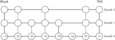
Figure 2: Skip list with $n=6$ nodes and $3$ levels.

Our dynamic distributed skip list data structure is architected using multiple “networks” (see Figure 3). Each peer node can participate in more than one network and in some cases more than one location within the same network. We use the following network structures.

The Spartan Network $\mathcal{S}$

is a wrapped butterfly network that contains all the current nodes. This network can handle heavy churn of up to $\mathcal{O}(n/\log n)$ nodes joining and leaving in every round [13]. However, this network is not capable of handling search queries.

Live Network $\mathcal{L}$

is the skip list network on which all queries are executed. Some of the nodes in this network may have left. We require such nodes to be temporarily represented by their replacement nodes (from their respective neighbors in $\mathcal{S}$).

Buffer Network $\mathcal{B}$

is a skip list network on which we maintain all new nodes that joined recently.

Clean Network $\mathcal{C}$

is a skip list network that seeks to maintain an updated version of the data structure that includes the nodes in the system.

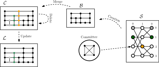
Figure 3: Schematic representation of the architecture and the Maintenance cycle described in Algorithm 1. Colored nodes in $\mathcal{L}$ and $\mathcal{C}$ are nodes that have been removed by the adversary and that are being covered by some committee of nodes (of the same color) in $\mathcal{S}$.

Moreover, in all skip lists, when a node exits the system, it is operated by a selected group of nodes. In the course of our algorithm description, if a node $u$ is required to perform some operation, but is no longer in the system, then its replacement node(s) will perform that operation on its behalf. Note further that some of the replacement nodes themselves may need to be replaced. Such replacement nodes will continue to represent $u$. The protocol assumes a short ($\Theta(\log n)$ round) initial “bootstrap” phase, where there is no churn and it initializes the underlying network. More precisely, the bootstrap is divided in two sub-phases in which we (i) build the underlying churn resilient network described in Section 2.1 in $\mathcal{O}(\log n)$ rounds and, (ii) we build the skip lists data structures $\mathcal{L}$ and $\mathcal{C}$ (initially $\mathcal{L}=\mathcal{C}$) using the $\mathcal{O}(\log n)$ rounds technique described in Section 2.4; after this, the adversary is free to exercise its power to add or delete nodes up to the churn limit and the network will undergo a continuous maintenance process. The overall maintenance of the dynamic distributed data structure goes through cycles. Each cycle $c\geq 1$ in Algorithm 1 is comprised of four phases. Without loss of generality assume that initially $\mathcal{L}$ and $\mathcal{C}$ are the same. We use the notation $\mathcal{L}^{(c)}$ (resp. $\mathcal{S}^{(c)},\mathcal{C}^{(c)},\mathcal{B}^{(c)}$) to indicate the network $\mathcal{L}$ (resp. $\mathcal{S},\mathcal{C},\mathcal{B}$) during the cycle $c\in\mathbb{N}$, when it is clear from the context we omit the superscript to maintain a cleaner exposition.

1

2Starting from a skip list $\mathcal{L}^{(1)}=\mathcal{C}^{(1)}$

3foreach Cycle $c\geq 1$ do

4      

5      Phase 1 (Deletion): All the replacement nodes in $\mathcal{C}^{(c)}$ are removed. Note that nodes that leave the system during the replacement process may remain in $\mathcal{C}^{(c)}$.

6      Phase 2 (Buffer Creation): All the new nodes that were churned into the system since Phase 2 of the previous cycle join together to form $\mathcal{B}^{(c)}$.

7      Phase 3 (Merge): The buffer $\mathcal{B}^{(c)}$ created in Phase $2$ is merged into $\mathcal{C}^{(c)}$, i.e., $\mathcal{C}^{(c+1)}\leftarrow\mathcal{C}^{(c)}\cup\mathcal{B}^{(c)}$.

8      Phase 4 (Update): Update the live network $\mathcal{L}^{(c)}$ with the clean network $\mathcal{C}^{(c)}$, i.e., $\mathcal{L}^{(c+1)}\leftarrow\mathcal{C}^{(c+1)}$.

9 end foreach

Algorithm 1 Overview of the distributed skip list maintenance process.

2.1 The Spartan network

A useful technique to build and maintain a stable overlay network that is resilient to a high amount of adversarial churn is to construct and maintain a network of (small-sized) committees [7, 9, 29, 13]. A committee is a clique of small ($\Theta(\log n)$) size composed of essentially “random” nodes. A committee can be efficiently constructed, and more importantly, maintained under large churn. Moreover, a committee can be used to “delegate” nodes to perform any kind of operation. In this work, to build and maintain our churn-resilient overlay network of committees we make use of the results in [13]. Our choice is motivated by two main advantages that the Spartan network in [13] has over the previous approach [29]: (a) it tolerates an abrupt adversarial churn rate of $\mathcal{O}(n/\log n)$, and (b) it can be built in $\mathcal{O}(\log n)$ rounds with high probability. Each committee is a dynamic random clique of size $\Theta(\log n)$ in which member nodes change continuously with the guarantee that the committee has $\Theta(\log n)$ nodes as its members at any given time. These committees are arranged into a wrapped butterfly network [53, 61]. The wrapped butterfly has $2^{k}$ rows and $k$ columns such that $k2^{k}\in\mathcal{O}(n/\log n)$ nodes and edges. The nodes correspond to committees and are represented by pairs $(r,\ell)$ where $\ell$ is the level or dimension of the committee ($0\leq\ell\leq k$) and $r$ is a $k$-bit binary number that denotes the row of the committee. Two committees $(r,\ell)$ and $(r^{\prime},\ell^{\prime})$ are linked by an edge that encodes a complete bipartite graph if and only if $\ell^{\prime}=\ell+1$ and either: (1) both committees are in the same row i.e., $r=r^{\prime}$, or (2) $r$ and $r^{\prime}$ differ in precisely the $(\ell+1(\text{mod }k))$th bit in their binary representation. Finally, the first and last levels of such network are merged into a single level. In particular, committee $(r,0)$ is merged into committee $(r,k)$. Figure 3 shows an example of Spartan network with $4$ rows and $2$ columns in which every node of the two-dimensional wrapped butterfly encodes a committee of $\Theta(\log n)$ random nodes and each edge between two committees encodes a complete bipartite graph connecting the vertices among committees. Notice that the first and last columns are the same set of committees since the butterfly is wrapped. The Spartan network is built during the bootstrap phase in which the adversary does not perform any move (having such phase is a common assumption in the DNC model [7, 8, 9, 10, 11, 13]). In [13], the authors showed how to efficiently build such wrapped butterfly of committees in $\mathcal{O}(\log n)$ rounds using $\mathcal{O}(\log n)$ messages per node at every round. For the sake of completeness, we provide a high-level description of how to build Spartan during the bootstrap phase. As a first step, a random node $v$ is elected as leader. Subsequently, a $\mathcal{O}(\log n)$ height binary tree rooted in $v$ is constructed. Next, the in-order traversal number for each node is computed and a cycle between the first $N=k2^{k}\in\mathcal{O}(n/\log n)$ nodes is created. Each node in such a cycle becomes a committee leader. The cycle is then transformed into a wrapped butterfly network with $k$ columns and $2^{k}$ rows. As a next step, the nodes that are not committee leaders randomly join one of the $N$ committees with the purpose to create committee of $\Theta(\log n)$ nodes. Once such committees are created, the nodes within each committee form a clique of size $\Theta(\log n)$. Finally, the committee leaders exchange the IDs of the nodes in their committee with their neighbors so that bipartite overlay edges can be formed between nodes in neighboring committees.

After the bootstrap phase, the nodes in Spartan run a continuous $\Theta(\log\log n)$ rounds maintenance cycle in which (1) all the nodes in the network move to another committee chosen uniformly at random among all the other committees and (2) the newly added nodes are assigned to random committees. This cycle prevents the powerful adversary to grasp sensitive information about the network structure and to replace all the nodes in the network. Augustine and Sivasubramaniam [13] showed that such a maintenance cycle makes the Spartan network robust with high probability against an adversarial churn rate of $\mathcal{O}(n/\log n)$, i.e., with high probability no committee is disrupted by the churn applied by oblivious adversary.

As a side contribution of our work, we generalize the Spartan protocol to handle an arbitrary number of nodes in the network, i.e., we relax the assumption that the size of the overlay network is fixed at each round to some number of nodes $n$. This makes the protocol adaptable to highly dynamic networks, in which the number of nodes might suddenly variate. We define a protocol that enlarges and reduces the dimensionality of $\mathcal{S}$ (i.e., reshapes $\mathcal{S}$) when the number of nodes in the Spartan network is such that the wrapped butterfly increases (resp. decreases) by one dimension. In Appendix C, we provide a reshaping protocol that reconfigures the Spartan network according to the number of peers present in the overlay network.

2.2 Replacing nodes that have been removed by the adversary

We describe how to maintain the live network $\mathcal{L}$ and the clean network $\mathcal{C}$ when churn occurs. Let us assume that a node $v\in V$ left the network. To preserve $\mathcal{C}$ and $\mathcal{L}$ structures, we require its committee in $\mathcal{S}$ “to cover” for the disappeared node. In other words, when a node $v$ leaves the network, its committee members in $\mathcal{S}$ will take care of all the operations involving $v$ in $\mathcal{L}$ and $\mathcal{C}$. Doing so, will temporarily preserve the structure of these networks, as if $v$ was still in the network. Moreover, we assume that at every round in the Spartan network, all the nodes within the same committee communicate their states (in $\mathcal{S},\mathcal{L}$, and $\mathcal{C}$) to all the other committee members, i.e., each node $u$ in a committee knows all its neighbors $N_{\mathcal{S}}(v)$, each neighbor in both skip list $\mathcal{L}$ and $\mathcal{C}$ for each $v\in N_{\mathcal{S}}(v)$, and all the committees of its neighbors in $\mathcal{L}$ and $\mathcal{C}$. Furthermore, when a node $v$ leaves the network, each node in its committee in $\mathcal{S}$ will connect to $v$’s neighbors in $\mathcal{L}$ and $\mathcal{C}$. This can be done in constant time and will increase the degree of the nodes in the data structures to $\mathcal{O}(\text{polylog}(n))$. Notice that each committee in $\mathcal{S}$ is guaranteed to be robust against a $\mathcal{O}(n/\log n)$ churn rate, i.e., the probability that there exists some committee of size $o(\log n)$ is at least $1/n^{d}$ for an arbitrarily large $d\geq 1$ (see Theorem 6 in [12]). This implies that every committee of nodes in $\mathcal{S}$ is able to cover for the removed nodes in $\mathcal{L}$ and $\mathcal{C}$ with high probability. Figure 4 shows an example of how the committees in the Spartan network cover for its members that were removed by the adversary. More precisely, in Figure 4(b) we show how the orange node’s committee is covering for it after being dropped by the adversary. An alternative way to see this is to assume that the committee creates a temporary virtual red node in place of the orange one (see Figure 4(c)).

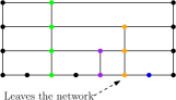
(a)

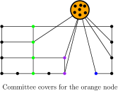
(b)

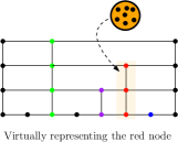
(c)

Figure 4: In Figure 4(a) the orange node gets removed by the adversary from the overlay network. Figure 4(b) shows how all its committee neighbors in the overlay cover for the orange node. Figure 4(c) is an equivalent visualization of Figure 4(b), the committee replaces the orange node with a “virtual” red node. This will temporarily preserve the skip list structure of Figure 4(a).

Lemma 2.1.

Replacing node(s) that have been removed by the adversary requires $\mathcal{O}(1)$ number of rounds and work proportional to the churn.

Proof 2.2.

When a node $v$ leaves the network, all its committee neighbors create an edge with $v$ neighbors in $\mathcal{L}$ and $\mathcal{C}$. This requires $\mathcal{O}(1)$ rounds and the amount of edge that are created by $v$’s committee is $\mathcal{O}(\log^{2}n)$ (at most $4\log n$ edges for each node in the $\mathcal{O}(\log n)$-sized committee). Observe that in one cycle of $\mathcal{O}(\log n)$ rounds we can experience a churn of $\mathcal{O}(n/\log n)$ at every time instant. Thus, the overall work is $\mathcal{O}(n\cdot\text{polylog}{(n)})$ and respects our dynamic resource competitiveness constraints.

2.3 Deletion

We describe how to safely clean the network $\mathcal{C}$ in $\mathcal{O}(\log n)$ rounds from the removed nodes for which committees in the Spartan network $\mathcal{S}$ are temporarily covering for. The elements in the clean network $\mathcal{C}$ before the cleaning procedure can be of two types: (1) not removed yet and (2) patched-up, i.e., nodes that have been removed by the adversary and for which another group of nodes in the network is covering for. A trivial approach to efficiently remove the patched-up nodes from $\mathcal{C}$, would be the one of destroying the clean network $\mathcal{C}$ by removing these nodes and then reconstructing the cleaned skip list from scratch. However, this approach does not satisfy our dynamic resource competitiveness constraint (see Definition 1.1 and Section 1.3); the effort we must pay to build the skip list from scratch may be much higher than the adversary’s total cost. Hence, we show an approach to clean $\mathcal{C}$ that guarantees dynamic resource competitiveness. For the sake of explanation, assume that the patched-up nodes are red and the one that should remain in $\mathcal{C}$ are black. The protocol is executed in all the levels of the skip list in parallel. The high-level idea of the protocol is to create a tree rooted in the skip list’s left-topmost sentinel by backtracking from some “special” leaves located on each level of the skip list. Once the rooted tree is constructed, another backtracking phase in which we build new edges connecting black nodes separated by a contiguous for its leaves is executed. Figure 5 shows an example of the delete routine (Algorithm 2) run on all the levels of the skip list in Figure 5(a). Moreover, Figure 5(b) and Figure 5(c) show the execution of the delete routine at level $0$. First, the tree rooted in the left-topmost sentinel is built by backtracking from the leaves (i.e., from the black nodes that have at least one red neighbor). Next, the tree is traversed again in a bottom-up fashion and green edges between black nodes separated by a list of red nodes are created (Figure 5(d)). Figure 5(e) depicts the skip list after after running Algorithm 2 in parallel on every level. Finally, Figure 5(f) shows the polished skip list.

1

Tree Formation Phase ($\mathcal{O}(\log n)$ rounds):

2Let $B$ be the set of black nodes at level $\ell$ with at least one red neighbor. In this step, we are required to form the shortest path tree $T$ rooted at the left-topmost sentinel with $B$ as its leaves. A simple bottom-up approach can be used to build this tree $T$ in $O(\log n)$ rounds.

 

Message Initialization ($(\mathcal{O}(1)$ rounds):

3Every $b\in B$ creates a message containing a pair of items as follows.

1.

$(\dot{b},\dot{b})$ if both its neighbors are red.

2.

$(\dot{b},b)$ if its left neighbor is red and its right neighbor is black

3.

$(b,\dot{b})$ if its left neighbor is black and its right neighbor is red

Each $b$ then sends its message to its parent in $T$.

 

Propagation Phase ($\mathcal{O}(\log n)$ rounds):

4This is executed by each node $u$ on the tree $T$. Node $u$ waits to hear messages from all its children. If it has only one child, it will propagate the message to its parent in the tree. Otherwise (i.e., it has two children) it receives two messages: $(w,x)$ from its child from below and $(y,z)$ from its child from its right. We will show later that either $x$ and $y$ are both dotted or neither of them are dotted.

5if both $x$ and $y$ are dotted then

6       Introduce $x$ to $y$ so that they can form an edge between them at level $\ell$.

7 end if

8Node $u$ then propagates the message $(w,z)$ to its parent on the tree.

Algorithm 2 Delete routine for level $\ell$. See Figure 5 for an illustration.

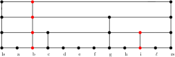
(a)

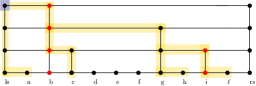
(b)

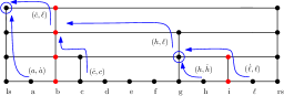
(c)

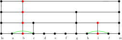
(d)

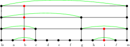
(e)

(f)

Figure 5: Example of the delete phase on a skip list. Red nodes are the one that must be deleted from the skip list, blue arrow indicates the path towards the left topmost sentinel in the skip list from the black nodes that wish wire-out its red neighbors. Figure 5(a) is the skip list before the deletion phase. Figure 5(b) shows the tree rooted in the left-topmost sentinel created by the Tree Formation Phase. Figure 5(c) shows the Message Initialization and the Propagation Phase executed at the bottom most level of the skip list where Blue circles indicate that an edge between two black nodes have been created. Figure 5(d) shows the skip list after the bottom most lever run Algorithm 2. Figure 5(e) is the skip list after running Algorithm 2 at all its levels. Finally, Figure 5(f) is the skip list after the deletion phase. The left and right sentinels are represented as ls and rs, respectively.

Lemma 2.3.

Algorithm 2 executed on a skip list at all levels $0\leq\ell\in\mathcal{O}(\log n)$ correctly creates an edge between every pair of black nodes that are separated by a set of red nodes at each level $\ell$ in $\mathcal{O}(\log n)$ rounds w.h.p.. Moreover, the total work performed by this procedure is within a $\text{polylog}(n)$ factor of the number of red nodes.

Proof 2.4.

We first establish a simple but useful invariant that holds for all nodes $u$ in $T$. Consider a pair $(x,y)$ propagated upwards by a node $u$ to its parent. We note that $x$ (resp., $y$) (in its un-dotted form) is the leftmost (resp., rightmost) leaf in the subtree rooted at $u$. This can be shown by induction. Clearly the statement is true if $u\in B$ as it creates the message to be of the form $(u,u)$ (either of them possibly dotted). The inductive step holds for $u$ at higher levels by the manner in which messages from children are combined at $u$.

Note that the procedure forms edges between pairs of nodes $(b,b^{\prime})$ at some level $\ell$ only if they are both in $B$ (corresponding to the execution pertaining to level $\ell$). Thus, for correctness, it suffices to show that the edge is formed if and only if all the nodes between $b$ and $b^{\prime}$ at level $\ell$ are red.

To establish the forward direction of the bidirectional statement, let us consider the formation of an edge $(b,b^{\prime})$ at some node $u$ that is at a level $\ell^{\prime}\geq\ell$. It coalesced two pairs of the form $(x,\dot{b})$ and $(\dot{b^{\prime}},y)$. The implication is that $b$ has a right neighbor at level $\ell$ that is red and $\dot{b}$ has a left neighbor at level $\ell$ that is red. Moreover, they are the rightmost leaf and left most leaf respectively of the subtrees rooted at $u$’s children. Thus, none of the nodes between $b$ and $b^{\prime}$ at level $\ell$ are in $T$. This implies that they must all be red nodes.

To establish the reverse direction, let us consider two nodes $b$ and $b^{\prime}$ at level $\ell$ that are both black with all nodes between them at level $\ell$ being red. Consider their lowest common ancestor $u$ in $T$. Clearly, $u$ must have two children, say, $v$ and $w$. From the invariant established earlier, the message sent by $v$ (resp., $w$) must be of the form $(\ast,\dot{b})$ (resp., $(\dot{b^{\prime}},\ast)$). Thus, $u$ must introduce $b$ and $b^{\prime}$, thereby forming the edge between them.

Since $T$ is the shortest path rooted at the left-topmost sentinel, its height is at most $\mathcal{O}(\log n)$ w.h.p. Both the tree formation and propagation phases are bottom-up procedures that take time proportional to the height of $T$. Thus, the total running time is $\mathcal{O}(\log n)$.

Finally, each node in $T$ sends at most $\mathcal{O}(1)$ messages up to its parent in $T$. This implies that the number of messages sent is proportional (within $\text{polylog}(n)$ factors) to the number of leaves in $T$. Also, all edges added in the tree are between pairs of nodes $(b,b^{\prime})$ in $B$ that are consecutive at level $\ell$ (i.e., no other node in $B$ lies between $b$ and $b^{\prime}$ at level $\ell$). Thus, work efficiency is established.

2.4 Buffer Creation

In this section, we outline the process of constructing the Buffer network $\mathcal{B}$, which comprises the nodes that have joined the network. Conceptually, to establish a skip list from an unsorted collection of distinct elements, the initial step involves creating the lowest level by organizing a sorted list. Subsequently, for each node in this list, a random experiment is conducted to construct the upper levels. In our context, we encounter an unsorted set of nodes $C$, which have been introduced into the Spartan network $\mathcal{S}$ through adversarial churn, and our objective is to construct a distributed skip list from it. Initially, our challenge lies in efficiently arranging these nodes to form the lowest level of the distributed data structure. The current best-known approach to sort $n$ elements using $\text{polylog}{(n)}$ incoming and outgoing messages for each node during each round requires $\mathcal{O}(\log^{3}n)$ time [6]. To improve on such result, we rely on sorting networks theory (e.g. [16, 1, 53]). A sorting network is a graph topology which is carefully manufactured for sorting. More precisely, it can be viewed as a circuit-looking DAG (directed acyclic graph) with $n$ inputs and $n$ outputs in which each node has exactly two inputs and two outputs (i.e., two incoming edges and two outgoing edges). A sorting network is such that for any input, the output is monotonically sorted. A sorting network is characterized by two parameters: the number of nodes resp. size and the depth. The space required to store a sorting network is determined by its size while the overall running time of the sorting algorithm is determined by its depth. Figure 6 shows an example of sorting network on $4$ elements.

(a)

(b)

(c)

(d)

Figure 6: Example of a sorting network [16] on $4$ numbers. Every crossing edge connecting two nodes in different levels is a node in the DAG representation. The upper output of a crossing edge connecting two nodes in different levels is the minimum between the two inputs, while the lower output is the maximum. Execution of the sorting network is left to right.

One notable construction for sorting $n$ elements is the $\mathcal{O}(\log n)$-depth (thus $\mathcal{O}(n\log n)$ size) AKS network, developed by Ajtai, Komlós, and Szemerédi [1] in the early $80$’s. However, a drawback of the AKS network is that the $\mathcal{O}(\cdot)$ notation hides large constant factors. Some progress has been made in simplifying the AKS network and improving the constant factors in its depth [66], but for practical values of $n$, the depth of Batcher’s bitonic sort [16] remains considerably smaller. Nevertheless, if we disregard the impracticability of the AKS network, we can improve the distributed sorting result in [6] by a $\mathcal{O}(\log^{2}n)$ factor. Moreover, it is well known that sorting networks can be simulated by a butterfly network and other hypercubic networks (see Chapter 3.5 in [53]). So, we first need to find a way to embed the AKS sorting network on a butterfly-like one. To this end, we use the result by Maggs and Vöcking [56] in which they show that an AKS network can be embedded on a multibutterfly [84]. A $k$-dimensional multibutterfly network consists of $k+1$ levels, each consisting of $2^{k}$ nodes. For $0\leq\ell\leq k$ and $0\leq i<2^{k}$, let $(\ell,i)$ be the label of the $\ell$th node on level $i$. The nodes on each level $\ell$ are partitioned into $2^{k}$ sets $A_{\ell,0},\dots,A_{\ell,2^{k}-1}$ where $A_{\ell,j}=\{(\ell,i):\lfloor i/2^{k-\ell}\rfloor=j\}$. The nodes in $A_{\ell,j}$ are connected to the nodes in $A_{\ell+1,2j}$ and $A_{\ell+1,2j+1}$. To embed the AKS network we need to consider a subclass of the multibutterfly networks that includes those multibutterfiles that can be constructed by superimposing butterfly networks. Furthermore, Maggs and Vöcking [56] showed how to embed the AKS network on what they called twinbutterfly, a multibutterfly obtained by superimposing two butterfly networks. On the twinbutterflty each leaf node has degree $4$ and each non-leaf node has degree $8$.

For completeness we state the result we are interested in.

Theorem 2.5 (Theorem 4.1 in [56]).

An AKS network $\mathcal{A}$ of size $N=\mathcal{O}(n\log n)$ can be embedded into a twinbutterfly $\mathcal{M}$ of size at most $\kappa\cdot N+o(N)$ with load $1$, dilation $2$, and congestion $1$, where $\kappa\leq 1.352$ is a small constant depending on the AKS parameters.

Here the load of an embedding is the maximum number of nodes of the AKS network mapped to any node of the twinbutterfly. The congestion is the maximum number of paths that use any edge in the twinbutterfly, and the dilation is the length of the longest path in the embedding. It follows that

Lemma 2.6.

There exists a distributed algorithm that builds a twinbutterfly network $\mathcal{M}$ in $\mathcal{O}(\log n)$ time.

Proof 2.7.

Let $n_{\mathcal{B}}=|C|$ be the number of nodes that must join together to form the Buffer network $\mathcal{B}$. The temporary twinbutterfly $\mathcal{M}$ can be built in $\mathcal{O}(\log n)$ rounds by adapting the distributed algorithm for building a butterfly network in [13] described in Section 2.1: (1) a leader $l$ is elected in $\mathcal{S}$; (2) a $\mathcal{O}(\log n)$ height binary tree rooted in $l$ is constructed; (3) a cycle using the first $n_{\mathcal{B}}(\log n_{\mathcal{B}}+1)$ nodes of the tree in-order traversal is built; and, (4) the cycle is then transformed into the desired twinbutterfly network with $\log n_{\mathcal{B}}+1$ columns and $n_{\mathcal{B}}$ rows in $\mathcal{O}(\log n)$ rounds.

The idea is to use such a butterfly construction algorithm to build a twinbutterfly $\mathcal{M}$ in $\mathcal{O}(\log n)$ rounds and simulate the AKS algorithm on it. Moreover, $\mathcal{M}$ being a data structure build on top of the Spartan network, it naturally enjoys a churn resiliency property. In fact, every time a node $v$ is churned out from $\mathcal{S}$, a committee will temporary cover for $v$ in $\mathcal{M}$ (see Section 2.2). Finally, we show that the $\mathcal{B}$ can be created in $\mathcal{O}(\log n)$ rounds.

Lemma 2.8.

The Creation phase can be computed in $\mathcal{O}(\log n)$ rounds w.h.p..

Proof 2.9.

$\mathcal{M}$ can be built in $\mathcal{O}(\log n)$ rounds (Lemma 2.6). Moreover, to handle cases in which $\kappa\cdot N+o(N)$ (see Theorem 2.5) is greater than the number of nodes in the Spartan network $\mathcal{S}$, we allow for nodes to represent a constant number of temporary “dummy” nodes for the sake of building the needed multibutterfly. Once $\mathcal{M}$ has been constructed, we run AKS on such network and after $\mathcal{O}(\log n_{\mathcal{B}})=\mathcal{O}(\log n)$ rounds we obtain the sorted list at the base of the new skip list we want to build. Next, each node $u$ in the buffer computes its maximum height $\ell_{\max}^{\mathcal{B}}(u)$ in the buffer skip list $\mathcal{B}$ and each level $0<\ell\leq\ell_{\max}(\mathcal{B})$ is created by copying the base level of the skip list. Moreover, each node $u$ at level $0<\ell\leq\ell_{\max}(\mathcal{B})$ can be of two types, effective or fill-in. We say that a node $u$ is effective at level $\ell$ if $\ell\leq\ell_{\max}^{\mathcal{B}}(u)$, and fill-in otherwise (see Figure 7(a)). Next, we use the same parallel $\mathcal{O}(\log n)$ rounds rewiring technique used in the Deletion phase (see Section 2.3) to exclude fill-in nodes from each level and obtain a skip list of effective nodes (see Figures 7(b)-7(c)). Wrapping up, to create the buffer network we need $\mathcal{O}(\log n)$ rounds to build the twibutterfly $\mathcal{M}$, $\mathcal{O}(\log n)$ rounds to run AKS on $\mathcal{M}$, $\mathcal{O}(\log n)$ rounds w.h.p. to duplicate the levels (see Lemma B.1 in Appendix B) and $\mathcal{O}(\log n)$ rounds to run the rewiring procedure. Thus, we need $\mathcal{O}(\log n)$ rounds w.h.p.

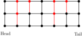
(a)

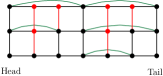
(b)

(c)

Figure 7: Example of create procedure. In Figure 7(a), freshly created Buffer network in which the black nodes are the effective nodes and red ones are the fill-in nodes. Figure 7(b) shows the buffer network after the parallel rewiring phase in which the green edges are the one created by the delete procedure. Finally, Figure 7(c) shows the buffer network after the Creation phase.

2.5 Merge

As a starting point, we analyze the process of inserting (in parallel) a sequence of sorted elements $X$ in a skip list $\mathcal{C}$. More precisely, each element $v\in X$ starts the insertion process in $\mathcal{C}$ at the same time and from the same spot. Intuitively, all these parallel insertions can be seen as a group of elements traveling all together in the skip list. We will use the term cohesive group to describe a group of elements traversing the skip list together. We define the leader of the cohesive group to be the element with the smallest ID/key among the group. In addition, the group is assumed to be small enough to ensure all nodes can exchange messages pairwise simultaneously in one round. While traversing the skip list, the leader is in charge of querying the newly encountered nodes and to communicate their ID/key to the cohesive group. Furthermore, it can happen that at some point a subset $X^{\prime}\subseteq X$ separates from $X$ and takes another route to level $0$. When such a split happens, say $X$ splits in two groups (see Proposition 2.10 below), the newly created cohesive group $X^{\prime}$ elects as a leader the element with the smallest ID/key in $X^{\prime}$. Note that such a split requires two rounds, one for the leader to inform all nodes in the new cohesive group who their leader is and one for the nodes in the new cohesive group to “introduce” themselves to their new leader.

Proposition 2.10.

Let $X=\{x_{0},x_{1},\dots,x_{k}\}$ where $x_{i-1}\leq x_{i}$ for $i\in[1,k]$ be a set of nodes that are traversing all together (i.e., a cohesive group) the skip list $\mathcal{C}$. And let $v\in X$ be a node that separates from $X$ at some time $t\geq 0$, then all $u\in X$ such that $u\geq v$ will separate from $X$ as well and will follow $v$.

Proof 2.11.

For the sake of contradiction, let $X=\{x_{0},x_{1},\dots,x_{k}\}$ where $x_{i-1}\leq x_{i}$ for $i\in[1,k]$ be a cohesive group that is traversing the skip list. Moreover, assume that $x_{j}$ separates from $X$ at some time $t$, and that there exists $x_{\ell}$ for $\ell\geq j$ that does not follow $x_{j}$, i.e., $x_{\ell}$ does not separate from $X$. This generates a contradiction on the assumption that the elements in $X$ are sorted in ascending order. Thus, it can not happen.

Finally, we show that the time to insert a cohesive group in a skip list is at most twice the time to insert a single element in the skip list.

Lemma 2.12.

Let $X=\{x_{0},x_{1},\dots,x_{k}\}$ where $x_{i-1}\leq x_{i}$ for $i\in[1,k]$ be a set of cohesive nodes that are inserted all together at the same time and from the top left sentinel node in a skip list $\mathcal{C}$. Then, the time to insert $x_{k}$ along with $x_{0},x_{1},\dots,x_{k-1},x_{k}$ is at most twice the time to insert just $x_{k}$.

Proof 2.13.

We prove this lemma by induction. The base case of the induction is the time needed to insert $x_{0}$ and the elements before $x_{0}$ in $X$, i.e., $\{\emptyset\}$. Observe that the time to insert $x_{0}$ is at most twice the time to insert $x_{0}$ because it is the first element in the set $X$ and its search path is $x_{0}$’s optimal search path in $\mathcal{C}$. The inductive hypothesis is that the time to insert $x_{k-1}$ along with $\{x_{0},x_{1},\dots,x_{k-1}\}$ is at most twice the time to insert $x_{k-1}$ and that $x_{k-1}$’s search path is the optimal search path when we insert only $x_{k-1}$ from the left top-most sentinel node. As inductive step, we consider the time needed to insert $x_{k}$ in $\mathcal{C}$. $x_{k}$’s search path can be divided in two regions: (i) a shared search path with $x_{k-1}$ and (ii) an independent path in which $x_{k}$ travels by itself until it reaches its destination. Moreover, observe that the shared region is a subset of the $x_{k}$’s optimal search path as well, otherwise (given that $x_{k-1}$ and $x_{k}$ perform the same moves) it would contradict the inductive hypothesis about $x_{k-1}$ search path optimality. As for the independent region, the correctness of the search/insert algorithm [68] implies that it must be a subset of the optimal search path as well. Finally, by combining the shared search path and the independent one we obtain that $x_{k}$’s overall search path must be the optimal one. Given that all the nodes move in parallel, we can conclude that the time to insert $x_{k}$ along $x_{0},x_{1},\dots,x_{k-1},x_{k}$ is at most twice the time to insert just $x_{k}$.

WAVE: An $\bm{\mathcal{O}(\log n)}$ merge procedure.

Here we show one of the main contributions of this paper. We provide a distributed protocol to merge two skip lists in $\mathcal{O}(\log n)$ rounds w.h.p. Intuitively, our merge procedure can be viewed as a top-down wave of parallel searches. The searches are performed on $\mathcal{C}$ by elements in $\mathcal{B}$. The wave is initiated by the top-most nodes in $\mathcal{B}$. At any point in time, the wave front represents all the nodes in $\mathcal{B}$ that are actively looking for the right position in $\mathcal{C}$. As nodes on the wave front find their respective appropriate location, they get inserted into $\mathcal{C}$. Thus, when the wave has swept through $\mathcal{C}$ in its entirety, we get the required merged skip list. Moreover, we notice that there must be only one cohesive group in the top level of the skip list $\mathcal{B}$, and that each couple of cohesive groups $X_{\ell},Y_{\ell}$ at the same level $\ell<\ell_{\max}(\mathcal{B})$ must be separated by one (or more) nodes $v$ that belongs to one (or more) cohesive group $Z_{\ell^{\prime}}$ such that $\ell^{\prime}>\ell$.

Proposition 2.14.

Given a skip list $\mathcal{B}$, there is only one cohesive group at $\ell_{\max}(\mathcal{B})$. Moreover, for each $0\leq\ell<\ell_{\max}(\mathcal{B})$, let $X_{\ell}=\{x_{0},x_{1},\dots,x_{k}\}$ be a cohesive group at level $\ell$. Then, $X_{\ell}$’s left neighbor (i.e. $x_{0}$’s left neighbor at level $\ell$) is a node $v$ such that $\ell_{\max}^{\mathcal{B}}(v)>\ell$.

Proof 2.15.

Let $\ell$ be the maximum height of the skip list $\mathcal{B}$ and assume to have two disjoint cohesive groups $X_{\ell}$ and $Y_{\ell}$. This implies that $X_{\ell}$ and $Y_{\ell}$ are separated by one (or more nodes) $v$ such that $\ell_{\max}^{\mathcal{B}}(v)>\ell$. Thus we have a contradiction on $\ell$ being $\mathcal{B}$’s maximum height. Next, let $0\leq\ell<\ell_{\max}(\mathcal{B})$, consider the cohesive group $X_{\ell}=\{x_{0},x_{1},\dots,x_{k}\}$ and its left neighbor $v$ at level $\ell$ (i.e., $v\in N_{\mathcal{B}}^{(L,\ell)}(x_{0})$). Then $v$ must be such that $\ell_{\max}^{\mathcal{B}}(v)>\ell$. That is because, if $\ell_{\max}^{\mathcal{B}}(v)=\ell$ then we would have $v\in X_{\ell}$ and if $\ell_{\max}^{\mathcal{B}}(v)<\ell$, we would have $v\notin N_{\mathcal{B}}^{(L,\ell)}(x_{0})$.

Before diving into the description of the WAVE protocol, we define the left and right children of a node $u$ at some level $\ell>0$ in a skip list. Informally, the right (resp. left) children of a node $u$ at level $\ell$ is defined by the set of contiguous nodes after (resp. before) $u$ at level $\ell$ in the skip list. Formally, given a node $u$ in the buffer network $\mathcal{B}$ at level $\ell>0$ we define $\Gamma_{\ell^{\prime}}^{L}(u)=\{v:v<u\land\ell_{\max}(v)=\ell^{\prime}\land\forall v<w<u,\ell_{\max}(w)\leq\ell^{\prime}\}$and $\Gamma_{\ell^{\prime}}^{R}(u)=\{v:v>u\land\ell_{\max}(v)=\ell^{\prime}\land\forall u<w<v,\ell_{\max}(w)\leq\ell^{\prime}\}$ as the left and right children of $u$ at level $\ell^{\prime}<\ell$ in $\mathcal{B}$. Moreover, we refer to $u$’s set of children at level $\ell^{\prime}$ as the union of its left and right ones at level $\ell^{\prime}$, i.e., $\Gamma_{\ell^{\prime}}{(u)}=\Gamma_{\ell^{\prime}}^{L}(u)\cup\Gamma_{\ell^{\prime}}^{R}(u)$ and to its overall set of children as the union of each $\Gamma_{\ell^{\prime}}{(u)}$ for all $\ell^{\prime}<\ell$ , i.e., $\Gamma{(u)}=\bigcup_{\ell^{\prime}=0}^{\ell-1}\Gamma_{\ell^{\prime}}{(u)}$. Furthermore, we notice that two neighboring nodes $u$ and $w$ at level $\ell$ share a subset of their children. In a similar way, we introduce the concept of parent of a node in a skip list. Given a node $u$ at some level $\ell<\ell_{\max}(\mathcal{B})$, we say that $z$ is a parent of $u$ if $u\in\Gamma{(z)}$. Observe that each node $u$ such that $\ell_{\max}(u)<\ell_{\max}(\mathcal{B})$ has exactly two parents. Figure 8 shows an example of the children-parent relationship defined above. The children set of a node $u$ can be seen as a depth $1$ tree rooted in $u$ where $u$’s children are its leaves (see Figure 8(b)).

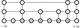
(a)

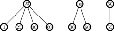
(b)

Figure 8: Example of the parent-children relationship defined above. Figure 8(a) is an example of a skip list. Figure 8(b) shows the children set $\Gamma$ of nodes $23$, $98$, and $60$, respectively.

The merge protocol is divided in two phases: (i) a preprocessing phase on the buffer network $\mathcal{B}$ and (ii) a merge phase on the clean network $\mathcal{C}$. The preprocessing phase takes care of creating the cohesive groups at each level that must be merged into $\mathcal{C}$ and to “shorten” the distance between every couple of nodes in such groups to guarantee fast communication time within the cohesive groups. More precisely, let $X_{\ell}=\{x_{0},x_{1},x_{2},\dots,x_{k}\}$ be a set of consecutive nodes such that $\ell_{\max}^{\mathcal{B}}(x)=\ell$ for each $x\in X_{\ell}$ and $0\leq\ell\leq\ell_{\max}(\mathcal{B})$. Then, each node $x_{i}\in X_{\ell}$ for $1\leq i\leq k$ sends its ID to $x_{0}$ through its left neighbor. Doing so will allow each $x_{i}$ to discover the ID of all the nodes $x_{j}\in X_{\ell}$ such that $x_{j}>x_{i}$ (see Figure 9). We observe that the preprocessing phase requires $\mathcal{O}(\log n)$ rounds w.h.p.

Lemma 2.16.

Given a skip list of $n$ nodes, the preprocessing phase requires $\mathcal{O}(\log n)$ rounds w.h.p.

(a)

(b)

(c)

Figure 9: Example of the preprocessing operation on a cohesive group of nodes. Figure 9(a), Figure 9(b) and Figure 9(c) show the cohesive group before, during, and after the preprocessing phase, respectively.

The proof of Lemma 2.16 follows from the fact that each $X_{\ell}$ for $0\leq\ell\leq\ell_{\max}(\mathcal{B})$ executes the protocol in parallel and that $|X_{\ell}|=\mathcal{O}(\log n)$ w.h.p. (see Lemma B.3 in Appendix B). Once the preprocessing phase is completed, the merge phase is executed. In such phase, each node in the buffer network $\mathcal{B}$ can be in one of the following three states $\{\texttt{idle, merge, done}\}$. Moreover, a node $u\in\mathcal{B}$ in idle state waits and keeps listening to its two parents in $\mathcal{B}$. A node in the merge state instead, is actively merging (as a leader or follower) itself in the clean network $\mathcal{C}$. Finally, a node that successfully merged in $\mathcal{C}$, enters the done state. Each node $u$ in the buffer network maintains a set of children $\Gamma(u)$, parents locations (initially set to $-\infty$), a starting point for its merge (initially set to $-\infty$), and the starting level for its own merge (initially set to be the topmost level in $\mathcal{C}$, i.e., $\ell_{\max}(\mathcal{C})$). Moreover, this concept nicely extends to a cohesive group of nodes that must travel together in the skip list $\mathcal{C}$. In the first round of the merge protocol, the unique cohesive group $X_{\ell_{\max}(\mathcal{B})}=\{x_{0},x_{1},\dots,x_{k}\}$ with $x_{0}=-\infty$ and $x_{k}=+\infty$ in $\mathcal{B}$’s topmost level changes its state to merge and starts its merging phase in $\mathcal{C}$ from the left-topmost sentry. For the sake of simplicity, we consider $\mathcal{B}$’s left and right sentries as nodes of the buffer network that must be merged with $\mathcal{C}$. We assume that such sentinels are contained in $\mathcal{C}$’s ones. Moreover, at each round, every cohesive group $X\subseteq\mathcal{B}$ on a node $v\in\mathcal{C}$ at level $\ell$ that is in the merge state performs the following steps:

1.

The leader $x_{0}$ checks node $v$’s ID/key in $\mathcal{C}$ on which $X$ is currently located;

2.

$x_{0}$ communicates $v$’s ID/key to its followers in $\mathcal{B}$, i.e., to the nodes in $X\setminus\{x_{0}\}$;

3.

$x_{0}$ computes the split $X^{\prime}=\{u\in V:u>z\}$ where $z$ is the right neighbor of $v$ at level $\ell$ and elects the element with smallest ID/key in $X^{\prime}$ as a leader of such new cohesive group;

4.

Each node $u\in\hat{X}$, where $\hat{X}=X\setminus X^{\prime}$, sends a message $m(u)=\langle v,z,\text{``down''},\ell\rangle$ to its children $\Gamma(u)$ in $\mathcal{B}$;

5.

Each node $w\in X^{\prime}$, sends a message $m(w)=\langle v,z,\text{``right''},\ell\rangle$ to its children $\Gamma(w)$ in $\mathcal{B}$;

6.

The new cohesive group $X^{\prime}$ separates from $X$ and continues its merge procedure on $z$ at level $\ell$;

7.

If the current level $\ell$ is at most $\ell_{\max}(x_{0})$, $\hat{X}$ must be merged between $v$ and $z$ in $\mathcal{C}$:

7.a.

$\hat{X}$ merges itself between $v$ and $z$;

7.b.

Each node $u\in\hat{X}$ sends a message $m(u)=\langle u,y,\text{``down''},\ell\rangle$ where $y$ is $u$’s right neighbor in the newly merged area that includes $v,\hat{X}$, and $z$ to $\Gamma(u)$;

7.c.

Each node in $u\in\hat{X}$ announces its successful merge at level $\ell$ to its children $\Gamma(u)$;

8.

If the next level $\ell-1\geq 0$, then $\hat{X}$ must proceed to the next level:

8.a.

If at least one of $\hat{X}$ neighbors at level $\ell$ is a node in $\mathcal{B}$, i.e., $\{v,z\}\cap\mathcal{B}\neq\emptyset$, then $\hat{X}$ waits for $\{v,z\}\cap\mathcal{B}$ to be merged at level $\ell-1$ and proceeds with its own merge at level $\ell-1$;

Furthermore, once a node is fully merged in level $0$ of $\mathcal{C}$, it enters the done state and terminates. Next, we describe the behavior of the nodes in $\mathcal{B}$ upon receiving messages from their parents. A node $v$, in the buffer network $\mathcal{B}$ in idle state is continuously listening to its parents. $v$’s behavior changes according to the type of message it is receiving. More precisely, let us assume that $v$ receives a message of the type $m(u)=\langle L,R,\texttt{move},\texttt{level}\rangle$ from its parent $u$:

If the message is sent by a node that is in the merge state at some level above $\ell_{\max}(v)$, then $v$ has to update its pointers:

1.

If $v<m(u).R$ and $v.\texttt{starting\_point}\leq m(u).L$ then $v$ updates its starting point and level for its own merge with the node $m(u).L$ and $m(u).\texttt{level}$, respectively;

2.

If $v>m(u).R$ and $v.\texttt{starting\_point}<m(u).R$ then $v$ updates its starting point and level for its own merge with the node $m(u).R$ and $m(u).\texttt{level}$, respectively;

3.

$v$ updates its parents locations according to the move their parents performed in $\mathcal{C}$, i.e., if $m(u).\texttt{move}=\text{``down''}$ then it updates the location of its parent $u$ with $m(u).L$, otherwise with $m(u).R$;

4.

Checks if it can enter in the merge state, this happens if $v$ becomes independent from its parents, i.e., if $v.\texttt{starting\_point}$ is different from the current location of both its parents in $\mathcal{C}$:

4.a.

$v$ looks at its left neighbor $z$ at level $\ell_{\max}(v)$ in $\mathcal{B}$. If $z$’s starting point is the same as $v$’s one, then $v$ sets itself as follower, otherwise $v$ becomes leader;

4.b.

If $v$ is leader, it enters in the merge state starting the merge procedure in $\mathcal{C}$ at $v.\texttt{starting\_point}$ and level $v.\texttt{level\_to\_start}$ along with its followers, i.e., the cohesive group $X=\{v\}\cup\{w:w\in N_{\mathcal{B}}^{(R,\ell_{\max}(v))}(v)\land v.\texttt{starting\_point}=w.\texttt{starting\_point}\}$ enters the merge state;

If $v$ is idle and discovers that both its parents successfully merged in $\mathcal{C}$ in level $\ell=\ell_{\max}(v)$, then it must change state to merge and proceed with its own merge phase in $\mathcal{C}$ starting from $v.\texttt{starting\_point}$ at level $v.\texttt{level\_to\_start}$. Moreover, as before, it:

1.

$v$ looks at its left neighbor $z$ at level $\ell_{\max}(v)$ in $\mathcal{B}$. If $z$’s starting point is the same as $v$’s one, then $v$ sets itself as follower, otherwise $v$ becomes leader;

2.

If $v$ is leader, it enters in the merge state starting the merge procedure in $\mathcal{C}$ at $v.\texttt{starting\_point}$ and level $v.\texttt{level\_to\_start}$ along with its followers, i.e., the cohesive group $X=\{v\}\cup\{w:w\in N_{\mathcal{B}}^{(R,\ell_{\max}(v))}(v)\land v.\texttt{starting\_point}=w.\texttt{starting\_point}\}$ enters the merge state;

First and foremost, we notice that all the idle nodes in $\mathcal{B}$ correctly update their starting points. More precisely, a node $v\in\mathcal{B}$ that updates its starting point, it can choose only another point laying in its optimal search path from the top-left sentry to $\mathcal{C}$’s bottom most level. This property follows by the fact that each node $v$ in $\mathcal{B}$ receives messages only by its (left and right) parents in $\mathcal{B}$, i.e., $v$ receives a list of nodes ID that lay on the optimal search paths of its parents in the skip list $\mathcal{C}^{\prime}=\mathcal{C}\cup\mathcal{B}_{>\ell}$ obtained by merging $\mathcal{C}$ and the elements of $\mathcal{B}$ situated in the level above $\ell$. Thus, $v$ updates its starting point with nodes that it would encounter had it performed a classic insertion in $\mathcal{C}^{\prime}$. Thus, $v$’s new starting point lays in its optimal search path. This property, allows the nodes in $\mathcal{B}$ to “virtually” travel in $\mathcal{C}$ using the information shared by their parents. Next, we notice that one critical part of our protocol is that a cohesive group $X$ that was successfully merged at some level $\ell$ and wants to proceed one level down to $\ell-1$ may have to wait for its parents $v$ and $z$ to be successfully merged in such target level. This happens if, at least one of $X$’s neighbors at level $\ell$ in $\mathcal{C}$ is an element in the buffer (i.e., it is one of its parents in $\mathcal{B}$) and it is still in its merging phase at level $\ell-1$. The next lemma provides a bound on the time a cohesive group $X$ needs to merge itself in the skip list provided that it may have to wait for its parents to be successfully merged beforehand at each level.

Lemma 2.17.

Let $X$ be a cohesive group at level $0\leq\ell\leq\ell_{\max}(\mathcal{B})$ in $\mathcal{B}$. The merge time of $X$ in $\mathcal{C}$ takes $\mathcal{O}(\log n+\ell_{\max}(\mathcal{B})-\ell)$ rounds w.h.p.

Proof 2.18.

Assume that the cohesive group $X$ was merged at level $\ell$ of the clean network and has to proceed with its own merge at level $\ell-1$. Let $v$ and $z$ be $X$’s left and right parents in $\mathcal{B}$. We have three cases to consider: (i) $X$ is independent from its parents; (ii) $X$ depends on at least one of its parents through all the levels $\ell^{\prime}<\ell$; and, (iii) $X$ may depend on one of its parents for some time and become independent at some point. In the first case, $X$ is merging itself in a sub-skip list that contains only elements in the clean network. Thus, $X$’s overall merging time requires $\mathcal{O}(\log n)$ w.h.p. To analyze the second case, we notice that as $X$ depends on its parents, also $X$’s parents may depend on their parents as well and so on. We can model the time a cohesive group $X$ at level $\ell$ has to wait in order to start its own merge procedure at level $\ell-1$ as the time it would have taken had it traveled in a pipelined fashion with its parents. Moreover, such pipelining effect can be extended to include, in a recursive fashion, the parents of $X$’s parents, the parents of the parents of $X$’s parents, and so on. Thus, $X$ can be modeled as the tail of such “parents-of-parents” chain (or pipeline), in which $X$ must wait for all the nodes in the pipeline to be merged at level $\ell-1$ before proceeding with its own merge in such level. Moreover, we observe that, by our assumption, $X$ is dependent on at least one of its parents throughout the merge phase. Without loss of generality, let us assume that $X$ depends on one parent, say $z$. In other words, $X$ is never splitting, and its placing itself right after/before $z$ at each level $\ell^{\prime}<\ell$. The time $X$ takes to merge in one level $\ell^{\prime}$ after $z$ is $\mathcal{O}(1)$ (see Lemma 2.12). Thus, $X$ merge itself in some level $\ell^{\prime}$ by time $T_{z}^{\ell^{\prime}}+\mathcal{O}(1)$ where $T_{z}^{\ell^{\prime}}$ is the time $z$ needs to merge itself in level $\ell^{\prime}$. Furthermore, $z$ may be dependent to one of its parents, say $w$. Thus the time to insert $z$ at level $\ell^{\prime}$ is $T_{z}^{\ell^{\prime}}=T_{w}^{\ell^{\prime}}+\mathcal{O}(1)$. If we repeat this argument for all the levels $\hat{\ell}>\ell^{\prime}$ we obtain that the time to merge the cohesive group $X$ at level $\ell^{\prime}$ can be defined as $T_{y}^{\ell^{\prime}}+\ell_{\max}(\mathcal{B})-\ell+1=T_{y}^{\ell^{\prime}}+\ell_{\max}(\mathcal{B})-\ell_{\max}^{\mathcal{B}}(X)+1$ where $y$ is the topmost parent in the pipeline of dependencies. Thus $X$’s overall merge time is $T_{X}^{0}=T_{y}^{0}+\ell_{\max}(\mathcal{B})-\ell_{\max}^{\mathcal{B}}(X)+1=\mathcal{O}(\log n+\ell_{\max}(\mathcal{B})-\ell_{\max}^{\mathcal{B}}(X)+1)$ w.h.p. In the last case, $X$ may depend on its parents for some time and then gain independency. Assume that $X$ depends its parent $z$ until level $\ell^{\prime}$ and than gains independency. $X$’s overall merge time is $T_{X}^{0}=\mathcal{O}(T_{z}^{\ell^{\prime}}+1+\log n)=\mathcal{O}(\log n)$ w.h.p.

Given Lemma 2.17, we can bound the overall running time of the WAVE protocol.

Lemma 2.19.

Let $\mathcal{C}$ and $\mathcal{B}$ be two skip lists of $n$ elements built using the same $p$-biased coin. Then, the WAVE protocol merges $\mathcal{C}$ and $\mathcal{B}$ in $\mathcal{O}(\log n)$ rounds w.h.p..

Proof 2.20.

The proof follows by noticing that a idle cohesive group $X$ in some level $\ell$ starts its merge procedure when the wave sweeps through it. This happens within $\mathcal{O}(\log n)$ rounds w.h.p. from the WAVE protocol initialization time instant. Moreover, a idle node/cohesive group, after entering the merge state needs $\mathcal{O}(\log n+\ell_{\max}(\mathcal{B})-\ell)$ rounds w.h.p. to be fully merged in $\mathcal{C}$ (Lemma 2.17). That is, the merge time is at most $\mathcal{O}(\log n+\log n+\ell_{\max}(\mathcal{B})-\ell)=\mathcal{O}(\log n)$ w.h.p.

Figure 10 shows an example of the WAVE protocol described above, each colored wave represent a round of the merging protocol.

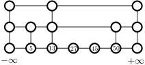
(a)

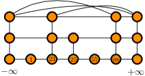
(b)

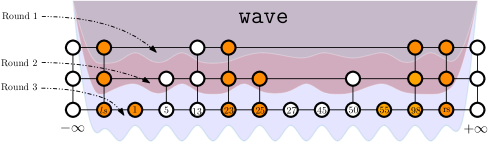
(c)

Figure 10: Example of the WAVE protocol. Figure 10(a) and Figure 10(b) show the clean network $\mathcal{C}$ (base skip list) and the preprocessed Buffer network $\mathcal{B}$, respectively. Figure 10(c) shows WAVE’s execution: light gray, light brown, and light blue waves are the first, second and third rounds of the protocol’s execution. After the last round, one step of rewiring is executed to remove the left and right sentries (ls, rs) from $\mathcal{C}$. In this example, the merging phase requires $\mathcal{O}(\log|\mathcal{B}|)$ rounds to merge the buffer network $\mathcal{B}$ with $\mathcal{C}$.

2.6 Update

After performing the previous phases, the live network $\mathcal{L}$ must be coupled with the newly updated clean network $\mathcal{C}$. A high level description on how to perform such update in constant time is the following: during the duplication phase a “snapshot” (e.g., a copy) of the clean network $\mathcal{C}$ is taken and used as the new $\mathcal{L}$. Intuitively, this procedure requires $\mathcal{O}(1)$ rounds because each node in $\mathcal{C}$ is taking care of the snapshot that can be considered as local computation. However, we must be careful with the notion of snapshot. To preserve dynamic resource-competitiveness we show how to avoid creating new edges while taking a snapshot of $\mathcal{C}$ during this phase. Assume that every edge in the clean network $\mathcal{C}$ has a length two local binary label $\lambda$ in which the first coordinate indicates its presence in $\mathcal{C}$ and the second one in $\mathcal{L}$. Moreover, each label $\lambda$ can be of three different types: (1) “$10$” the edge is in $\mathcal{C}$ not in $\mathcal{L}$; (2) “$01$” the edge is not in $\mathcal{C}$ but it is in $\mathcal{L}$; and, (3) “$11$” the edge is in both $\mathcal{C}$ and $\mathcal{L}$. Moreover, assume that each node $u$ in $\mathcal{C}$ has the label $\lambda(u,v)$ associated to its port encoding the connection with node $v$. Then, each node $u$ in $\mathcal{C}$ for each $0\leq\ell\leq\ell_{\max}(u)$ performs the following local computation:

1.

If $u$’s port-label associated to the edge connected to the left neighbor at level $\ell$ (i.e., $\lambda(u,v)$ such that $v\in N_{\mathcal{C}}^{(L,\ell)}(u)$) is “$10$” then set it to “$11$”;

2.

If $u$’s port-label associated to the edge connected to the right neighbor at level $\ell$ (i.e., $\lambda(u,w)$ such that $w\in N_{\mathcal{C}}^{(R,\ell)}(u)$) is “$10$” then set it to “$11$”;

Notice that during this phase no edge has the label “$01$” because $\mathcal{C}$ was “cleaned” during the deletion phase. All the nodes in $\mathcal{C}$ executed the labeling procedure, and the live network $\mathcal{L}$ is given by the edges with label “$11$”. It follows that this phase requires a constant number of rounds.

Lemma 2.21.

The update phase requires constant number of rounds.

Next, we show that all the phases in the maintenance cycle satisfy the dynamic resource competitiveness constraint defined in Section 1.3.

Lemma 2.22.

Each maintenance cycle is $(\alpha,\beta)$-dynamic resource competitive with $\alpha=\mathcal{O}(\log n)$ and $\beta=\mathcal{O}(\text{polylog}{(n)})$.

Proof 2.23.

In order to prove that our maintenance protocol is dynamic resource competitive we suffice to show that a generic iteration of our maintenance cycle respects this invariant.

Let $t_{s}$ be the time instant in which the deletion phase starts, and let $t_{e}=\mathcal{O}(t_{s}+\log n)$. The overall churn between the previous deletion phase and the current one is $C(t_{s}-\mathcal{O}(\log n),t_{s})=\mathcal{O}(n)$, that is because we have $\mathcal{O}(n/\log n)$ churn at each round for $\mathcal{O}(\log n)$ rounds. The total amount messages sent during the phase is $\tilde{\mathcal{O}}(C(t_{s}-\mathcal{O}(\log n),t_{s}))$ and the number of formed edges is $\tilde{\mathcal{O}}(C(t_{s}-\mathcal{O}(\log n),t_{s}))$. Thus the overall amount of work during the deletion phase is $\mathcal{W}(t_{s},t_{e})=\tilde{\mathcal{O}}(C(t_{s}-\mathcal{O}(\log n),t_{s}))$.

During the buffer creation phase, we create a twin-butterfly network $\mathcal{M}$ in $\mathcal{O}(\log n)$ rounds using $\mathcal{O}(\log n)$ messages for each node at every round. Moreover, the twinbutterfly has $\mathcal{O}(n\log n)$ nodes of which $2n$ nodes have degree $4$ while the rest have degree $8$. This implies that while building the twinbutterfly we create roughly $\mathcal{O}(n\log n)$ edges and we exchange $\mathcal{O}(n\log^{2}n)$ messages. Next, during each round of the AKS algorithm, each node $u$ in $\mathcal{M}$ sends and receives a constant number of messages. Then, we copy such a list $\mathcal{O}(\log n)$ times w.h.p., in this way we create $\mathcal{O}(n\log n)$ edges. Finally, in the last step of the buffer creation phase, we run the deletion algorithm used in the previous phase on a subset of the nodes in the sorted list. Putting all together, during this phase, we have an overall amount of work of $\mathcal{W}(t_{s},t_{e})=\mathcal{O}(C(t_{s}-\mathcal{O}(\log n),t_{s})\cdot\text{polylog}{(n)})=\tilde{\mathcal{O}}(C(t_{s}-\mathcal{O}(\log n),t_{s}))$.

During the merge phase, we merge the buffer network with the clean one. The preprocessing step creates $\mathcal{O}(n\log n)$ edges on the buffer network using at most $\text{polylog}{(n)}$ number of messages. During each step of the WAVE protocol sends $\mathcal{O}(n\cdot\text{polylog}{(n)})$ overall number of messages on the buffer network and creates $\mathcal{O}(n\log n)$ edges in the clean network. Putting all together, we have that the merge phase does not violate our dynamic work efficiency requirements. Indeed the overall work is bounded by $\mathcal{W}(t_{s},t_{e})=\mathcal{O}(C(t_{s}-\mathcal{O}(\log n),t_{s})\cdot\text{polylog}{(n)})=\tilde{\mathcal{O}}(C(t_{s}-\mathcal{O}(\log n),t_{s}))$.

Finally, during the duplication phase there is no exchange of messages and no edge is created.

We have that each phase of the maintenance cycle does not violate our resource competitiveness requirements in Definition 1.1.

We conclude by showing that the skip list is maintained with high probability for $n^{c}$ rounds, where $c\geq 1$ is an arbitrary big constant.

Lemma 2.24.

The maintenance protocol ensures that the resilient skip list is maintained effectively for at least $poly(n)$ rounds with high probability.

Proof 2.25.

Each phase of the maintenance protocol (i.e., Algorithm 1) succeeds with probability at least $1-\frac{1}{n^{c}}$, for some arbitrary big constant $c\geq 1$. Let $X$ be a geometric random variable of parameter $p=\frac{1}{n^{c}}$ that counts the number of cycle needed to have the first failure, then its expected value is $\mathbb{E}\left[X\right]=n^{c}$, for $c\geq 1$. Moreover, the probability of maintenance protocol succeeding in a round $n^{r}$ for some $r<c$ is $(1-\frac{1}{n^{c}})^{n^{r}}$, Without loss of generality assume $c>1$ and $r=c-1$, then $(1-\frac{1}{n^{c}})^{n^{c-1}}\leq e^{-n^{c-1}/n^{c}}\geq 1-\frac{1}{n}$.

Proof of the Main Theorem (Theorem 1.2).

To prove the main theorem it is sufficient to notice that the skip list will always be connected and will never loose its structure thanks to Lemma 2.1. Indeed, every time a group of nodes is removed from the network, there are committees that in $\mathcal{O}(1)$ rounds will take over and act on their behalf. This allows all the queries to go through without any slowdown. Thus all the queries will be executed in $\mathcal{O}(\log n)$ rounds with high probability even with a churn rate of $\mathcal{O}(n/\log n)$ per round. Next we can show that the distributed data structure can be efficiently maintained using maintenance cycles of $\mathcal{O}(\log n)$ rounds each. To do this, it is sufficient to show that each phase of our maintenance cycle (Algorithm 1) can be carried out in $\mathcal{O}(\log n)$ rounds (see Lemma 2.3, Lemma 2.8, Lemma 2.19, and Lemma 2.21). Moreover, from Lemma 2.22 we have that each phase is $(\alpha,\beta)$-dynamic resource competitive with $\alpha=\mathcal{O}(\log n)$ and $\beta=\mathcal{O}(\text{polylog}{(n)})$. Finally, the maintenance protocol ensures that the distributed data structure is maintained for at least $n^{c}$ rounds with high probability where $c\geq 1$ is an arbitrarily large constant.

2.7 Extending our approach to other data structures

The outlined maintenance protocol provides a convenient framework for constructing churn-resilient data structures. Furthermore, it can be easily adapted to maintain a more complex distributed pointer based data structure such as a skip graphs [44, 3, 39, 47]. Indeed, with minor adjustments to the phases outlined in Algorithm 1, a maintenance cycle capable of maintain such data structures against heavy churn rate can be devised. To this end, we briefly discuss how to adapt our results to skip graphs. A skip graph [3], can be viewed as an extension of skip lists. Indeed, both consists of a set of increasingly sparse doubly-linked lists ordered by levels starting at level $0$, where membership of a particular node $u$ in a list at level $\ell$ is determined by the first $\ell$ bits of an infinite sequence of random bits associated with $u$, referred to as the membership vector of $u$, and denoted by $m(u)$. Let the first $\ell$ bits of $m(u)$ as $m(u)|\ell$. In the case of skip lists, level $\ell$ has only one list, for each $\ell$, which contains all elements $u$ such that $m(u)|\ell=1^{\ell}$, i.e., all elements whose first $\ell$ coin flips all came up heads. Skip graphs, instead, have $2^{\ell}$ lists at level $\ell$, which we can index from $0$ to $2^{\ell}-1$. Node $u$ belongs to the $j$-th list of level $\ell$ if and only if $m(u)|\ell$ corresponds to the binary representation of $j$. Hence, each node is present in one list of every level until it eventually becomes the only member of a singleton list. Without loss of generality, assume that the skip graph has sentry nodes as classical skip lists. Thus, the skip graph can be maintained as follows:

Deletion.

We can use the same $\mathcal{O}(\log n)$ rounds approach described in Section 2.3 to remove from the clean skip graph the nodes that have left the network.

Buffer Creation.

To build the base level of the buffer skip graph we can use the same $\mathcal{O}(\log n)$ rounds approach described in Section 2.4. While, to construct the skip graph from level $0$, we build an “augmented” skip list in which each node $u$ in each level $\ell$ is identified by its ID/key and the list $j$ at level $\ell$ in which $u$ appears (there are $2^{\ell}$ lists at level $\ell$). Thus, each node $u$ at some level $\ell$ can be: (i) effective in the list $j$ and fill-in for the remaining $i\neq j$, for $j,i\in[1,2^{\ell}]$; or, (ii) fill-in in all the lists $j\in[1,2^{\ell}]$. Finally, such augmented skip list is transformed into a skip graph by running (in parallel) Algorithm 2 in Section 2.3 on each level $\ell$ for which there exists at least one fill-in node.

Merge.

We can use the same merge phase described in Section 2.5, with the only difference that a node $u$ in the merge state at some level $\ell$, must be merged in one of the $2^{\ell}$ list in such level.

Duplicate.

We can use the same approach described in Section 2.6.

Consequently, we can claim a similar result to Theorem 1.2 for skip graphs. In essence, with small changes in the delete, buffer creation, merge and update algorithms, our maintenance algorithm can be tailored to the specific data structure in question. Thus, making our approach ideal for building complex distributed data structures in highly dynamic networks.

2.8 Extending our approach to deal with multiple keys on each node

Throughout the paper we assumed that each node in the network posses exactly one element of the data structure. This assumption can be relaxed to deal with multiple keys on each node. Indeed, in the case in which in the network there are $t\cdot n$ keys, where $t>0$, all the techniques described above allow to maintain the data structure in the presence of the same adversarial churn rate.

Corollary 2.26.

Given a network with $n$ nodes in which each vertex $v$ possesses $t$ elements in the skip list for some $t>1$. Then maintenance protocol requires $\mathcal{O}(t\cdot\log n)$ rounds to build and maintain a resilient skip list that can withstand heavy adversarial churn at a churn rate of up to $\mathcal{O}(n/\log n)$ nodes joining/leaving per round.

3 Concluding remarks and discussion

In this work we proposed the first churn resilient skip list that can tolerate a heavy adversarial churn rate of $\mathcal{O}(n/\log n)$ nodes per round. The data structure can be seen as a four networks architecture in which each network plays a specific role in making the skip list resilient to churns and keeping it continuously updated. Moreover, we provided efficient $\mathcal{O}(\log n)$ rounds resource competitive algorithms to (i) delete a batch of elements from a skip list (ii) create a new skip list and, (iii) merge together two skip lists. This last result is the first algorithm that can merge two skip list (as well as a skip list and a batch of new nodes) in $\mathcal{O}(\log n)$ rounds w.h.p.. We point out that these algorithms can be easily adapted to work on skip graphs [3, 39, 47].

In a broader sense, our technique is general and can be used to maintain any kind of distributed data structure despite heavy churn rate. The only requirement is to devise efficient delete, buffer creation, merge, and update algorithms for the designated data structure.

An additional contribution of our work is the improvement on the $\mathcal{O}(\log^{3}n)$ rounds state-of-the-art technique for sorting in the $\text{NCC}_{0}$ model. We show how to sort $n$ elements (despite a high churn rate) in $\mathcal{O}(\log n)$ rounds using results for sorting network theory. However, given the impracticability of the AKS sorting network, our result is purely theoretical. In practice, it could be easily implemented using Batcher’s network instead of the AKS one. This change would slow down the bootstrap phase and the maintenance cycle to $\mathcal{O}(\log^{2}n)$ rounds.

Finally, given the simplicity of our approach, we believe that our algorithms could be used as building blocks for other non-trivial distributed computations in dynamic networks.

Appendix

Appendix A Useful Mathematical Tools

In Appendix C, we use the Chernoff bound for the Poisson trials

Theorem A.1 (Theorem 4.4 [61]).

Let $X$ be a sum of $n$ independent Poisson trials $X_{i}$ such that , for $i\in[n]$. Then,

$$\text{for }R\geq 6\mathbb{E}\left[X\right]$$ (1)

Moreover, to provide high confidence bounds for the properties of randomized skip list we use the following tools.

Theorem A.2 (Right tail).

Let $X$ be a sum of $n$ independent random variables $X_{i}$ such that $X_{i}\in[0,1]$. Let $\mathbb{E}\left[X\right]=\mu$. Then,

$$\text{for }k>\mu$$ (2)

$$\text{for }\varepsilon\geq 0$$ (3)

Theorem A.3 (Left tail).

Let $X$ be a sum of $n$ independent random variables $X_{i}$ such that $X_{i}\in[0,1]$. Let $\mathbb{E}\left[X\right]=\mu$. Then,

$$\text{for }k<\mu$$ (4)

$$\text{for }\varepsilon\in(0,1)$$ (5)

Furthermore, a useful result about the upper tail value of a negative binomial distribution to a lower tail value of a suitably defined binomial distribution that allows us to use all the results for lower tail estimates of the binomial distribution to derive upper tails estimate for negative binomial distribution. This a very nice result because finding bounds for the right tail of a negative binomial distribution directly from its definition is very difficult.

Theorem A.4 (See Chapter $4$ in [71]).

Let $X$ be a negative binomial random variable with parameters $r$ and $p$. Then, where $Y$ is a binomial random variable with parameters $n$ and $p$.

Appendix B Useful Skip list properties

Lemma B.1.

The height of a $n$-element skip list is $\mathcal{O}(\log n)$ w.h.p.

Proof B.2.

Let $Y_{i}$ for $i\in[n]$ be the random variable that counts the number of consecutive heads we obtain while tossing a p-biased coin before we get a tail. Moreover, define $h$ to be the maximum height of the skip list i.e., $h=1+\max\{Y_{i}:i\in[n]\}$. Observe that , and that by a straightforward application of the union bound we obtain the probability of having a skip list of height at least $k$, . Choosing $k=4\log_{1/p}n+1$, we obtain a high confidence bound for the number of levels in the distributed data structure Moreover, $h$’s expected values is

$$\mathbb{E}\left[h\right]=\sum_{i>0}$$ (7)

$$\leq 4\log n+np^{4\log n}\left(\sum_{i\geq 1}p^{i-1}\right)=4\log n+n\left(\frac{1}{n^{4}}\right)\left(\frac{1}{1-p}\right)\leq 4\log n+1=\mathcal{O}(\log n)$$ (8)

Where the last inequality holds if the $\log$ is in base $1/p$ and if $n$ is sufficiently large.

Next, we say that $X_{\ell}=\{x_{1},x_{2},\dots,x_{k}\}$ is a run/cohesive group of nodes in a skip list $\mathcal{L}$ at level $\ell$, if $X_{\ell}$ is a set of consecutive nodes such that $\ell_{\max}^{\mathcal{L}}(x_{i})=\ell$ for each $x_{i}\in X_{\ell}$. Moreover, we give a high confidence bound on the size of a run $X_{\ell}$.

Lemma B.3.

The size of a run of nodes $X_{\ell}$ for some level $\ell$, is at most $\mathcal{O}(\log n)$ w.h.p., and its expected value is $1/(1-p)$.

Proof B.4.

The size of a run of nodes $|X_{\ell}|$ is a geometric random variable with parameter $1-p$. Thus, Choosing $k=c\log_{1-p}n+1$ for $c\geq 1$, gives us a high confidence bound on the number of consecutive nodes in a run of node $X_{\ell}$ at some level $\ell$. Indeed, Moreover, its expected value is $\mathbb{E}\left[|X_{\ell}|\right]=1/(1-p)$, assuming $p=1/2$ (in other words, constant), we have that the expected length of a run of nodes at some level $\ell$ of the skip list is $\mathcal{O}(1)$.

Finally, we conclude with the analysis of the search/deletion/insertion of an element in a skip list (see Figure 11 for an example about one of these operations).

Lemma B.5.

The running time for an insertion, deletion and search of an element in a skip list takes $\mathcal{O}(\log n)$ rounds w.h.p.

Proof B.6.

Let $R_{i}$ be number of horizontal edges at level $0\leq i\leq h$ crossed by a search operation that starts on the left topmost node of the skip list. Define the random variable $W_{h}=|R_{0}|+|R_{1}|+\dots+|R_{h}|$ to be the amount of horizontal moves performed by the search algorithm. Observe that each $R_{i}$ is a geometric random variable of parameter $1-p$ and that $h$ is a random variable itself. From Lemma B.1 we know that $\mathbb{E}\left[h\right]=\mathcal{O}(\log n)$ and that . Since $h$ is a random variable, $W_{h}$ is a random sum of random variables thus we can not make a straightforward use of the properties of sum of geometric random variables, rather we can write:

$$\leq\sum_{h=0}^{4\log n}$$ (12)

We notice that $W_{4\log n}$ is a deterministic sum of geometric random variables. Hence we can use the relation between the upper tail value of a negative binomial distribution and the lower tail value of a suitably defined binomial distribution to derive upper tail estimates for the negative binomial distribution (see Appendix A). Thus, we rewrite as where $Y$ is a binomial random variable with parameter $n=16\log n$ and $p$. Now, we apply a Chernoff bound [61] and by setting $k=4\log n$, $p=1/2$ and $\mu=8\log n$ we obtain

$$=\left(\frac{16}{27}\right)^{4\log n}\leq\frac{1}{n^{3}}$$ (14)

Therefore, Now that we have derived a high confidence bound for $W_{h}$ we can obtain a bound for its expected value:

$$\mathbb{E}\left[W_{h}\right]=\sum_{i=1}^{16\log n}$$ (16)

Observe that the first sum is bounded above $16\log n$ because every probability is less than $1$ and the second one is dominated by $\sum_{i\geq 1}1/i^{2}$ which is a constant. Since the running time of a search operation is bounded by the number of horizontal moves performed at each level plus the number of vertical moves to reach the target node from the topmost level to the bottom most. We have that the overall running time of a search procedure starting at the left topmost node in the skip list is $T=h+W_{h}=\mathcal{O}(\log n)$ with probability at least $1-(1/n^{2})$, by applying the union bound we have that $T$ is $\mathcal{O}(\log n)$ with probability at least $1-(1/n)$ starting at any node in the skip list. To conclude, the expected running time is $\mathbb{E}\left[T\right]=\mathbb{E}\left[h\right]+\mathbb{E}\left[W_{h}\right]=\mathcal{O}(\log n)$.

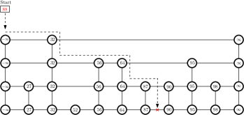
Figure 11: Example of the insertion of the element $88$ in the skip list. Dashed line is the search path.

Appendix C Spartan’s Reshaping protocol

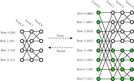
Figure 12: Example of the reshaping procedure. On the left, the Spartan structure as a one-dimensional wrapped butterfly of committees. The rows are represented with their binary representations. Every node in the figure is a random committee of $\Theta(\log n)$ nodes and every edge between two committees encodes a complete bipartite graph. On the right, $2$-dimensional butterfly is obtained by increasing the dimensionality of the left-wrapped butterfly by one. Green nodes are the ones that must be added to increase the dimensionality of the $1$-dimensional wrapped butterfly. Moreover, left-to-right execution increases the dimensionality by one, and right-to-left execution decreases the dimensionality by one.

In this section, we provide a detailed description of the reshaping protocol mentioned in Section 2.1. Let $\alpha,\beta\in\mathbb{R}_{\geq 0}$ such that $\alpha>1$ and $\beta\in(0,1)$ be two constants. We want the Spartan network $\mathcal{S}$ to be enlarged if all the committees have size at most $\alpha c\log n$, to shrink if all the committees have size at most $\beta c\log n$, or stay the same otherwise ($c>0$ is the constant hidden by the asymptotic notation). In other words, we want $\mathcal{S}$ to be enlarged or reduced when the wrapped butterfly network size increases or decreases by one dimension respectively. Moreover, a general technique to increase the dimensionality of a $k$-dimensional butterfly network $\mathcal{S}$ by one is to: (1) create a copy of $\mathcal{S}$ in which each row ID $(i,j)$ is “shifted” by $2^{k}$ i.e., $(2^{k}+i,j)$; (2) “shift” the index of the levels of the two disjoint butterflies by one; (3) add a new row of $2^{k+1}$ nodes to form the level $0$ of the $k+1$ dimensional butterfly; and, (5) connect the newly created level $0$ to the two disjoint butterflies using the “standard” butterfly edge-construction rule [53]. Furthermore, to reduce the dimensionality of a $k$-dimensional butterfly, we need to remove the level $0$, remove one of the two disjoint $k-1$-dimensional butterflies, and fix the row and levels IDs if needed. Figure 12 shows an example on how to perform such operations. We start with the description of the growing procedure. A new number of nodes $n^{\prime}=\alpha n$ is reached such that $2^{k}k\in\mathcal{O}(N)$ must be increased to $2^{k+1}(k+1)\in\mathcal{O}(N^{\prime})$ (the number of committees increases from $N=\mathcal{O}(n/\log n)$ to $N^{\prime}=\mathcal{O}(n^{\prime}/\log n^{\prime})$) and update the butterfly structure according to the new size of the network. Moreover, each step of Algorithm 3 requires at most $\mathcal{O}(\log n)$ rounds and no node will send or receive more than $\mathcal{O}(\log n)$ messages at any round. As a first step, the committee $C(0,0)$ is elected as a leader, and each committee routes a message in which it expresses its opinion (grow, shrink, stay the same) to the leader committee (lines 1-2). This can be done very efficiently on hypercubic networks [53, 61], indeed we have that the leader committee will receive all the opinions in $\mathcal{O}(\log N)$ rounds [54] where $N\in\mathcal{O}(n/\log n)$ is the number of committees in the wrapped butterfly. If the network agrees on growing, the protocol proceeds with increasing the dimensionality of the wrapped butterfly by one. Moreover, assume that the $k$-dimensional butterfly must be transformed into a $k+1$-dimensional one. To this end, the protocol executes the growing approach described before. Every committee shifts its level ID by one and promotes two random nodes in each committee to be the committee leaders of the copy of the butterfly and of the new level $0$. Next, all the newly elected committee leaders will start recruiting random nodes in the network until they reach a committee size of $\Theta(\log n^{\prime})$ where $n^{\prime}=\alpha n$. Finally, each new committee will create edges according to the wrapped butterfly construction algorithm [53, 13] and drop the old ones (if any). The next lemma shows that the growing phase requires $\mathcal{O}(\log n^{\prime})$ rounds w.h.p. where $n^{\prime}=\alpha n$.

Lemma C.1.

The network growth process ensures that every committee has $\Theta(\log n^{\prime})$ members after $\mathcal{O}(\log n^{\prime})$ rounds w.h.p.

Proof C.2.

Let $b=\frac{3n^{\prime}}{4N^{\prime}}=\frac{3}{4}\log n^{\prime}$ we show that after the first phase of the process, each new committee with gain $b$ nodes. During each round, there are at least $\frac{n^{\prime}}{4}-N^{\prime}\in\Omega(n^{\prime})$ nodes that did not receive any invitation from one of these new committee leaders. Moreover, define the event $E_{v}=\text{``The committee leader {v} recruits a node''}$ then setting $N^{\prime}=\frac{n^{\prime}}{c\log n^{\prime}}$ with $c\geq 1$ gives . To bound the expected time needed by a committee to recruit $b$ elements we define a pure-birth Markov Chain $\{X_{t}\}_{t\geq 0}$ with state space $\Omega=\{0,1,2,\dots,b\}$ and initial state $0$ that counts the number of recruited members. At each round, the Markov Chain at state $i<b$ can proceed one step forward to state $i+1$ with probability $p_{i,i+1}=$ or loop on $i$ with probability $r_{i,i}=1-p_{i,i+1}$. Observe that each state $0\leq i<b$ is a transient state, while $b$ is an absorbing state, and that the expected absorption time in state $b$ is $\mathcal{O}(b)=\mathcal{O}(\log n^{\prime})$. To give a tail bound on the absorption time, we study a more pessimistic random process in which we toss a p-biased coin with $p=3/16$ and count the number of rounds $Z_{i}$ before we get $b$ heads. In this experiment, the expected number of rounds needed to get $b$ heads is $\frac{16}{3}b\in\Theta(\log n^{\prime})$. By applying a Chernoff bound (Theorem A.1) we can show that for any value of $n^{\prime}$ and any fixed $R$, such that $R\geq 6\mathbb{E}\left[Z\right]$ the probability that we will need more than $R\log n^{\prime}$ rounds to get $b$ number of heads is at most $1/n^{\prime R}$. In other words, this means that the Markov Chain will take at most $\mathcal{O}(\log n^{\prime})$ rounds with probability $1-1/n^{\prime R}$ to reach state $b$. Finally, by applying the union bound we can show that every committee will need $\mathcal{O}(\log n^{\prime})$ rounds with probability $1-1/n^{\prime R-1}$ to recruit $b$ members.

Furthermore, in the case in which the network agreed on shrinking i.e., reducing the butterfly dimensionality from $k$ to $k-1$ a pool of vacated nodes $\mathcal{V}$ is created and all the nodes in the level $0$ and in the committees $C(i,j)$ such that $2^{k-1}\leq i<2^{k}$ and $1\leq j\leq k$ join such pool of nodes. Next, each committee in the remaining butterfly network will “recruit” $b=\frac{3}{4}\log n^{\prime}$ (here $n^{\prime}=\beta n$) random nodes from $\mathcal{V}$. After the recruitment phase, each remaining node $u$ in $\mathcal{V}$ (if any) will probe a random committee in the butterfly. If such a committee has not reached the target size yet it accepts the request, otherwise $u$ tries again with a different committee. It follows that the shrinking phase can be done in $\mathcal{O}(\log n^{\prime})$ rounds w.h.p. where $n^{\prime}=\beta n$.

Lemma C.3.

The network shrinking process ensures that every committee has $\Theta(\log n^{\prime})$ members after $\mathcal{O}(\log n^{\prime})$ rounds w.h.p.

Proof C.4.

Let $b=\frac{3n^{\prime}}{4N^{\prime}}=\frac{3}{4}\log n^{\prime}$ and observe that the analysis of the recruitment phase is identical to the one for the growing process. Moreover, after $\Theta(\log n)$ rounds, there can be $n^{\prime}/4$ nodes in $\mathcal{V}$ that are not part of any committee. Each node that joined a committee has one unit of budget that can use to induce a new member into its committee. Every remaining node $u\in\mathcal{V}$ probes a random node $v$ asking to join its committee, if $v$’s budget is greater than $0$ then $v$ accepts the request, otherwise $u$ tries again with a different node. Furthermore, observe that even if all the remaining nodes $\mathcal{V}$ found a spot in some committee, there will be $n^{\prime}/2$ nodes that would not have exhausted their budget and each remaining node can find a committee with probability at least $1/2$. Finally, by using similar arguments to the growing process we can show that each remaining node $u$ succeed in finding a committee with high probability in $\Theta(\log n^{\prime})$ rounds. And by using the union bound we can guarantee that each remaining node can find and become part of a committee in $\Theta(\log n^{\prime})$ w.h.p.

1

Agreement Phase.

2The committee $C(0,0)$ is elected as a leader $\ell$.

3Every committee in $\mathcal{S}$ routes its opinion to $\ell$.

4if Agreement on Growing then

5      

      Growing Phase.;

        // Here $n^{\prime}=\alpha n$

      

6      Each committee $C(i,j)$ for $0\leq i<2^{k}$ and $0\leq j<k$:

7      (a) Increases its committee ID from $C(i,j)$ to $C(i,j+1)$.

8      

9      (b) Promotes a random node $u$ among the available committee members to be the leader of the new committee $C(j\cdot 2^{k-1}+i,0)$.

10      

11      (c) Promotes a random node $v$ among the available committee members to be the leader of the new committee $C(2^{k-1}+i,j+1)$.

12      

13      Each newly generated committee leader actively recruits new nodes in their committee until it gets $\Theta(\log n^{\prime})$ committee members.

14      Each new committee creates complete bipartite edges according to the Wrapped Butterfly construction algorithm (see [53, 13]).

15else if Agreement on Shrinking then

       Shrinking Phase. ;

        // Here $n^{\prime}=\beta n$

      

16      Each member in the committees $C(i,0)$ for $0\leq i<2^{k}$ and $C(i,j)$ for $2^{k-1}\leq i<2^{k}$ $1\leq j\leq k$ “vacate” its committee and joins a pool of unassigned nodes.

17      Each node in the pool of unassigned nodes will randomly join one of the $N^{\prime}=\mathcal{O}(n^{\prime}/\log n^{\prime})$ new committees such that each committee has $\Theta(\log n^{\prime})$ nodes.

18else

19      

20      Do nothing.

21 end if

Algorithm 3 Reshape protocol.

References

- [1] Miklós Ajtai, János Komlós, and Endre Szemerédi. An o(n log n) sorting network. In Proceedings of the 15th Annual ACM Symposium on Theory of Computing, 25-27 April, 1983, Boston, Massachusetts, USA. ACM, 1983.
- [2] Dana Angluin, James Aspnes, Jiang Chen, Yinghua Wu, and Yitong Yin. Fast construction of overlay networks. In SPAA 2005: Proceedings of the 17th Annual ACM Symposium on Parallelism in Algorithms and Architectures, July 18-20, 2005, Las Vegas, Nevada, USA. ACM, 2005.
- [3] James Aspnes and Gauri Shah. Skip graphs. ACM Trans. Algorithms, 2007.
- [4] James Aspnes and Udi Wieder. The expansion and mixing time of skip graphs with applications. Distributed Comput., 2009.
- [5] Hagit Attiya, Sweta Kumari, Archit Somani, and Jennifer L. Welch. Store-collect in the presence of continuous churn with application to snapshots and lattice agreement. Inf. Comput., 2022.
- [6] John Augustine, Keerti Choudhary, Avi Cohen, David Peleg, Sumathi Sivasubramaniam, and Suman Sourav. Distributed graph realizations. IEEE Trans. Parallel Distributed Syst., 2022.
- [7] John Augustine, Anisur Rahaman Molla, Ehab Morsy, Gopal Pandurangan, Peter Robinson, and Eli Upfal. Storage and search in dynamic peer-to-peer networks. In 25th ACM Symposium on Parallelism in Algorithms and Architectures, SPAA ’13, Montreal, QC, Canada - July 23 - 25, 2013. ACM, 2013.
- [8] John Augustine, Gopal Pandurangan, and Peter Robinson. Fast byzantine agreement in dynamic networks. In ACM Symposium on Principles of Distributed Computing, PODC ’13, Montreal, QC, Canada, July 22-24, 2013. ACM, 2013.
- [9] John Augustine, Gopal Pandurangan, and Peter Robinson. Fast byzantine leader election in dynamic networks. In Distributed Computing - 29th International Symposium, DISC 2015, Tokyo, Japan, October 7-9, 2015, Proceedings. Springer, 2015.
- [10] John Augustine, Gopal Pandurangan, Peter Robinson, Scott T. Roche, and Eli Upfal. Enabling robust and efficient distributed computation in dynamic peer-to-peer networks. In IEEE 56th Annual Symposium on Foundations of Computer Science, FOCS 2015, Berkeley, CA, USA, 17-20 October, 2015. IEEE Computer Society, 2015.
- [11] John Augustine, Gopal Pandurangan, Peter Robinson, and Eli Upfal. Towards robust and efficient computation in dynamic peer-to-peer networks. In Proceedings of the Twenty-Third Annual ACM-SIAM Symposium on Discrete Algorithms, SODA 2012, Kyoto, Japan, January 17-19, 2012. SIAM, 2012.
- [12] John Augustine and Sumathi Sivasubramaniam. Spartan: A framework for sparse robust addressable networks. In 2018 IEEE International Parallel and Distributed Processing Symposium, IPDPS 2018, Vancouver, BC, Canada, May 21-25, 2018. IEEE Computer Society, 2018.
- [13] John Augustine and Sumathi Sivasubramaniam. Spartan: Sparse robust addressable networks. J. Parallel Distributed Comput., 2021.
- [14] Baruch Awerbuch and Christian Scheideler. The hyperring: a low-congestion deterministic data structure for distributed environments. In Proceedings of the Fifteenth Annual ACM-SIAM Symposium on Discrete Algorithms, SODA 2004, New Orleans, Louisiana, USA, January 11-14, 2004. SIAM, 2004.
- [15] Özalp Babaoglu, Moreno Marzolla, and Michele Tamburini. Design and implementation of a P2P cloud system. In Proceedings of the ACM Symposium on Applied Computing, SAC 2012, Riva, Trento, Italy, March 26-30, 2012. ACM, 2012.
- [16] Kenneth E. Batcher. Sorting networks and their applications. In American Federation of Information Processing Societies: AFIPS Conference Proceedings: 1968 Spring Joint Computer Conference, Atlantic City, NJ, USA, 30 April - 2 May 1968, AFIPS Conference Proceedings. Thomson Book Company, Washington D.C., 1968.
- [17] Luca Becchetti, Andrea Clementi, Emanuele Natale, Francesco Pasquale, and Luca Trevisan. Finding a bounded-degree expander inside a dense one. In Proceedings of the 2020 ACM-SIAM Symposium on Discrete Algorithms, SODA 2020, Salt Lake City, UT, USA, January 5-8, 2020. SIAM, 2020.
- [18] Luca Becchetti, Andrea E. F. Clementi, Francesco Pasquale, Luca Trevisan, and Isabella Ziccardi. Expansion and flooding in dynamic random networks with node churn. Random Struct. Algorithms, 2023.
- [19] Michael A. Bender, Jeremy T. Fineman, Mahnush Movahedi, Jared Saia, Varsha Dani, Seth Gilbert, Seth Pettie, and Maxwell Young. Resource-competitive algorithms. SIGACT News, 2015.
- [20] Ankur Bhargava, Kishore Kothapalli, Chris Riley, Christian Scheideler, and Mark Thober. Pagoda: a dynamic overlay network for routing, data management, and multicasting. In SPAA 2004: Proceedings of the Sixteenth Annual ACM Symposium on Parallelism in Algorithms and Architectures, June 27-30, 2004, Barcelona, Spain. ACM, 2004.
- [21] Inc BitTorrent. Website of bittorrent. https://www.bittorrent.com/, last checked on 14-February-2024.
- [22] John F. Canny. Collaborative filtering with privacy. In 2002 IEEE Symposium on Security and Privacy, Berkeley, California, USA, May 12-15, 2002. IEEE Computer Society, 2002.
- [23] Soumyottam Chatterjee, Gopal Pandurangan, and Nguyen Dinh Pham. Distributed MST: A smoothed analysis. In ICDCN 2020: 21st International Conference on Distributed Computing and Networking, Kolkata, India, January 4-7, 2020. ACM, 2020.
- [24] Inc Cloudmark. Website of cloudmark. https://cloudmark.com/, last checked on 14-February-2024.
- [25] Inc Crashplan. Website of crashplan. https://crashplan.com/, last checked on 14-February-2024.
- [26] Souptik Datta, Kanishka Bhaduri, Chris Giannella, Ran Wolff, and Hillol Kargupta. Distributed data mining in peer-to-peer networks. IEEE Internet Comput., 2006.
- [27] Luc Devroye. A limit theory for random skip lists. The Annals of Applied Probability, 1992.
- [28] Shlomi Dolev. Self stabilization. Journal of Aerospace Computing, Information, and Communication, 2004.
- [29] Maximilian Drees, Robert Gmyr, and Christian Scheideler. Churn- and dos-resistant overlay networks based on network reconfiguration. In Proceedings of the 28th ACM Symposium on Parallelism in Algorithms and Architectures, SPAA 2016, Asilomar State Beach/Pacific Grove, CA, USA, July 11-13, 2016. ACM, 2016.
- [30] Peter Druschel and Antony I. T. Rowstron. PAST: A large-scale, persistent peer-to-peer storage utility. In Proceedings of HotOS-VIII: 8th Workshop on Hot Topics in Operating Systems, May 20-23, 2001, Elmau/Oberbayern, Germany. IEEE Computer Society, 2001.
- [31] Jarret Falkner, Michael Piatek, John P. John, Arvind Krishnamurthy, and Thomas E. Anderson. Profiling a million user dht. In Proceedings of the 7th ACM SIGCOMM Internet Measurement Conference, IMC 2007, San Diego, California, USA, October 24-26, 2007. ACM, 2007.
- [32] Keir Fraser. Practical lock-freedom. Technical report, University of Cambridge, Computer Laboratory, 2004.
- [33] Joaquim Gabarró and Xavier Messeguer. A unified approach to concurrent and parallel algorithms on balanced data structures. In Proceedings 17th International Conference of the Chilean Computer Science Society. IEEE, 1997.
- [34] Joaquim Gabarró Vallès, Conrado Martínez Parra, and Xavier Messeguer Peypoch. A top-down design of a parallel dictionary using skip lists. Theoretical Computer Science, 1994.
- [35] Robert G. Gallager, Pierre A. Humblet, and Philip M. Spira. A distributed algorithm for minimum-weight spanning trees. ACM Trans. Program. Lang. Syst., 1983.
- [36] Prasanna Ganesan and Gurmeet Singh Manku. Optimal routing in chord. In Proceedings of the Fifteenth Annual ACM-SIAM Symposium on Discrete Algorithms, SODA 2004, New Orleans, Louisiana, USA, January 11-14, 2004. SIAM, 2004.
- [37] Roxana Geambasu, Tadayoshi Kohno, Amit A. Levy, and Henry M. Levy. Vanish: Increasing data privacy with self-destructing data. In 18th USENIX Security Symposium, Montreal, Canada, August 10-14, 2009, Proceedings. USENIX Association, 2009.
- [38] Robert Gmyr, Kristian Hinnenthal, Christian Scheideler, and Christian Sohler. Distributed monitoring of network properties: The power of hybrid networks. In 44th International Colloquium on Automata, Languages, and Programming, ICALP 2017, July 10-14, 2017, Warsaw, Poland, LIPIcs. Schloss Dagstuhl - Leibniz-Zentrum für Informatik, 2017.
- [39] Michael T. Goodrich, Michael J. Nelson, and Jonathan Z. Sun. The rainbow skip graph: a fault-tolerant constant-degree distributed data structure. In Proceedings of the Seventeenth Annual ACM-SIAM Symposium on Discrete Algorithms, SODA 2006, Miami, Florida, USA, January 22-26, 2006. ACM Press, 2006.
- [40] Thorsten Götte, Kristian Hinnenthal, and Christian Scheideler. Faster construction of overlay networks. In Structural Information and Communication Complexity - 26th International Colloquium, SIROCCO 2019, L’Aquila, Italy, July 1-4, 2019, Proceedings, Lecture Notes in Computer Science. Springer, 2019.
- [41] Thorsten Götte, Kristian Hinnenthal, Christian Scheideler, and Julian Werthmann. Time-optimal construction of overlay networks. In PODC ’21: ACM Symposium on Principles of Distributed Computing, Virtual Event, Italy, July 26-30, 2021. ACM, 2021.
- [42] P. Krishna Gummadi, Stefan Saroiu, and Steven D. Gribble. A measurement study of napster and gnutella as examples of peer-to-peer file sharing systems. Comput. Commun. Rev., 2002.
- [43] Kathrin Hanauer, Monika Henzinger, and Christian Schulz. Recent advances in fully dynamic graph algorithms - A quick reference guide. ACM J. Exp. Algorithmics, 2022.
- [44] Nicholas J. A. Harvey, Michael B. Jones, Stefan Saroiu, Marvin Theimer, and Alec Wolman. Skipnet: A scalable overlay network with practical locality properties. In 4th USENIX Symposium on Internet Technologies and Systems, USITS’03, Seattle, Washington, USA, March 26-28, 2003. USENIX, 2003.
- [45] Ragib Hasan, Zahid Anwar, William Yurcik, Larry Brumbaugh, and Roy H. Campbell. A survey of peer-to-peer storage techniques for distributed file systems. In International Symposium on Information Technology: Coding and Computing (ITCC 2005), Volume 2, 4-6 April 2005, Las Vegas, Nevada, USA. IEEE Computer Society, 2005.
- [46] Maurice Herlihy, Yossi Lev, Victor Luchangco, and Nir Shavit. A provably correct scalable concurrent skip list. In Conference On Principles of Distributed Systems (OPODIS). Citeseer, volume 103, 2006.
- [47] Riko Jacob, Andréa W. Richa, Christian Scheideler, Stefan Schmid, and Hanjo Täubig. Skip: A self-stabilizing skip graph. J. ACM, 2014.
- [48] Tim Jacobs and Gopal Pandurangan. Stochastic analysis of a churn-tolerant structured peer-to-peer scheme. Peer-to-Peer Netw. Appl., 2013.
- [49] M. Frans Kaashoek and David R. Karger. Koorde: A simple degree-optimal distributed hash table. In Peer-to-Peer Systems II, Second International Workshop, IPTPS 2003, Berkeley, CA, USA, February 21-22,2003, Revised Papers, Lecture Notes in Computer Science. Springer, 2003.
- [50] Peter Kirschenhofer, Conrado Martinez, and Helmut Prodinger. Analysis of an optimized search algorithm for skip lists. Theor. Comput. Sci., 1995.
- [51] Peter Kirschenhofer and Helmut Prodinger. The path length of random skip lists. Acta Informatica, 1994.
- [52] Fabian Kuhn, Stefan Schmid, and Roger Wattenhofer. Towards worst-case churn resistant peer-to-peer systems. Distributed Comput., 2010.
- [53] F Thomson Leighton. Introduction to parallel algorithms and architectures: Arrays· trees· hypercubes. Elsevier, 2014.
- [54] Frank Thomson Leighton, Bruce M. Maggs, Abhiram G. Ranade, and Satish Rao. Randomized routing and sorting on fixed-connection networks. J. Algorithms, 1994.
- [55] Eng Keong Lua, Jon Crowcroft, Marcelo Pias, Ravi Sharma, and Steven Lim. A survey and comparison of peer-to-peer overlay network schemes. IEEE Commun. Surv. Tutorials, 2005.
- [56] Bruce M. Maggs and Berthold Vöcking. Improved routing and sorting on multibutterflies. Algorithmica, 2000.
- [57] David J. Malan and Michael D. Smith. Host-based detection of worms through peer-to-peer cooperation. In Proceedings of the 2005 ACM Workshop on Rapid Malcode, WORM 2005, Fairfax, VA, USA, November 11, 2005. ACM Press, 2005.
- [58] Dahlia Malkhi, Moni Naor, and David Ratajczak. Viceroy: a scalable and dynamic emulation of the butterfly. In Proceedings of the Twenty-First Annual ACM Symposium on Principles of Distributed Computing, PODC 2002, Monterey, California, USA, July 21-24, 2002. ACM, 2002.
- [59] Gurmeet Singh Manku, Mayank Bawa, and Prabhakar Raghavan. Symphony: Distributed hashing in a small world. In 4th USENIX Symposium on Internet Technologies and Systems, USITS’03, Seattle, Washington, USA, March 26-28, 2003. USENIX, 2003.
- [60] Inc Microsoft. Website of skype. https://www.skype.com/, last checked on 14-February-2024.
- [61] Michael Mitzenmacher and Eli Upfal. Probability and computing: Randomization and probabilistic techniques in algorithms and data analysis. Cambridge university press, 2017.
- [62] Moni Naor and Udi Wieder. Novel architectures for P2P applications: The continuous-discrete approach. ACM Trans. Algorithms, 2007.
- [63] Gopal Pandurangan, Prabhakar Raghavan, and Eli Upfal. Building low-diameter P2P networks. In 42nd Annual Symposium on Foundations of Computer Science, FOCS 2001, 14-17 October 2001, Las Vegas, Nevada, USA. IEEE Computer Society, 2001.
- [64] Gopal Pandurangan, Peter Robinson, and Amitabh Trehan. DEX: self-healing expanders. Distributed Comput., 2016.
- [65] Thomas Papadakis, J. Ian Munro, and Patricio V. Poblete. Analysis of the expected search cost in skip lists. In SWAT 90, 2nd Scandinavian Workshop on Algorithm Theory, Bergen, Norway, July 11-14, 1990, Proceedings, Lecture Notes in Computer Science. Springer, 1990.
- [66] Mike Paterson. Improved sorting networks with o(log N) depth. Algorithmica, 1990.
- [67] Arjan Peddemors. Cloud storage and peer-to-peer storage-end-user considerations and product overview. GigaPort3 deliverable, 2010.
- [68] William Pugh. Skip lists: a probabilistic alternative to balanced trees. Communications of the ACM, 1990.
- [69] William Pugh. Concurrent maintenance of skip lists. In Technical Report, 1998.
- [70] Sylvia Ratnasamy, Paul Francis, Mark Handley, Richard Karp, and Scott Shenker. A scalable content-addressable network. In Proceedings of the 2001 conference on Applications, technologies, architectures, and protocols for computer communications, 2001.
- [71] Sheldon M Ross, Sheldon M Ross, Sheldon M Ross, and Sheldon M Ross. A first course in probability. Macmillan New York, 1976.
- [72] Antony I. T. Rowstron and Peter Druschel. Pastry: Scalable, decentralized object location, and routing for large-scale peer-to-peer systems. In Middleware 2001, IFIP/ACM International Conference on Distributed Systems Platforms Heidelberg, Germany, November 12-16, 2001, Proceedings, Lecture Notes in Computer Science. Springer, 2001.
- [73] Antony I. T. Rowstron and Peter Druschel. Storage management and caching in past, A large-scale, persistent peer-to-peer storage utility. In Proceedings of the 18th ACM Symposium on Operating System Principles, SOSP 2001, Chateau Lake Louise, Banff, Alberta, Canada, October 21-24, 2001. ACM, 2001.
- [74] Antony I. T. Rowstron, Anne-Marie Kermarrec, Miguel Castro, and Peter Druschel. SCRIBE: the design of a large-scale event notification infrastructure. In Networked Group Communication, Third International COST264 Workshop, NGC 2001, London, UK, November 7-9, 2001, Proceedings, Lecture Notes in Computer Science. Springer, 2001.
- [75] Subhabrata Sen and Jia Wang. Analyzing peer-to-peer traffic across large networks. IEEE/ACM Trans. Netw., 2004.
- [76] Nir Shavit and Itay Lotan. Skiplist-based concurrent priority queues. In Proceedings of the 14th International Parallel & Distributed Processing Symposium (IPDPS’00), Cancun, Mexico, May 1-5, 2000. IEEE Computer Society, 2000.
- [77] Inc Signal. Website of signal. https://signal.org/, last checked on 14-February-2024.
- [78] Ion Stoica, Robert Tappan Morris, David R. Karger, M. Frans Kaashoek, and Hari Balakrishnan. Chord: A scalable peer-to-peer lookup service for internet applications. In Proceedings of the ACM SIGCOMM 2001 Conference on Applications, Technologies, Architectures, and Protocols for Computer Communication, August 27-31, 2001, San Diego, CA, USA. ACM, 2001.
- [79] Ion Stoica, Robert Tappan Morris, David Liben-Nowell, David R. Karger, M. Frans Kaashoek, Frank Dabek, and Hari Balakrishnan. Chord: a scalable peer-to-peer lookup protocol for internet applications. IEEE/ACM Trans. Netw., 2003.
- [80] Daniel Stutzbach and Reza Rejaie. Understanding churn in peer-to-peer networks. In Proceedings of the 6th ACM SIGCOMM Internet Measurement Conference, IMC 2006, Rio de Janeriro, Brazil, October 25-27, 2006. ACM, 2006.
- [81] Håkan Sundell and Philippas Tsigas. Scalable and lock-free concurrent dictionaries. In Proceedings of the 2004 ACM Symposium on Applied Computing (SAC), Nicosia, Cyprus, March 14-17, 2004. ACM, 2004.
- [82] Inc Sysform. Website of sysform. https://symform.com/, last checked on 14-February-2024.
- [83] Thomas Tseng, Laxman Dhulipala, and Guy E. Blelloch. Batch-parallel euler tour trees. In Proceedings of the Twenty-First Workshop on Algorithm Engineering and Experiments, ALENEX 2019, San Diego, CA, USA, January 7-8, 2019. SIAM, 2019.
- [84] Eli Upfal. An o(log(n)) deterministic packet-routing scheme. J. ACM, 1992.
- [85] Leslie G. Valiant. A scheme for fast parallel communication. SIAM J. Comput., 1982.
- [86] Vasileios Vlachos, Stephanos Androutsellis-Theotokis, and Diomidis Spinellis. Security applications of peer-to-peer networks. Comput. Networks, 2004.
- [87] Inc Wikipedia. Wikipedia page about gnutella. https://en.wikipedia.org/wiki/Gnutella, last checked on 14-February-2024.
- [88] Ben Y. Zhao, John Kubiatowicz, and Anthony D. Joseph. Tapestry: a fault-tolerant wide-area application infrastructure. Comput. Commun. Rev., 2002.