Properties of a trapped multiple-species bosonic mixture at the infinite-particle-number limit: A solvable model

Abstract

Trapped mixtures of Bose-Einstein condensates have attracted much attention. The properties of such mixtures are rather difficult to compute and analyze. This statement applies the more, the more species are involved. We investigate a trapped mixture of Bose-Einstein condensates consisting of a multiple number of P species. To be able to do so, an exactly-solvable many-body model is called into play. This is the $P$-species harmonic-interaction model. After presenting the Hamiltonian, the ground-state energy and wavefunction are explicitly calculated. The solution is facilitated by utilizing a double set of Jacoby coordinates, the first is a set of relative-motion Jacoby coordinates for each of the species and the second is a set of Jacoby coordinates built from the center-of-mass coordinates of the $P$ species. All properties of the mixture’s ground state can in principle be obtained from the many-particle wavefunction. A scheme to integrate the all-particle density matrix is derived and implemented, leading to closed-form expressions for the reduced one-particle density matrices. Of particular interest is the infinite-particle-number limit, which is obtained when the numbers of bosons are taken to infinity while keeping the interaction parameters fixed. We first prove that at the infinite-particle-number limit all the species are $100\%$ condensed. The mean-field solution of the $P$-species mixture is also obtained analytically, and is used to show that the energy per particle and densities per particle computed at the many-body level of theory boil down to their mean-field counterparts. Despite these, correlations in the mixture exist at the infinite-particle-number limit. The availability of the solvable model allows one to enter an uncharted ground and explore how correlations of a bosonic mixture at the infinite-particle-number limit depend on the interactions and, in particular, on the number of species $P$ in the mixture. To this end, we obtain closed-form expressions for the correlation energy, namely, the difference between the mean-field and many-body energies, and the depletion of the species, i.e., the number of particles residing outside the condensed modes, at the infinite-particle-number limit. The depletion and the correlation energy per species are shown to critically depend on the number of species. Of separate interest is the entanglement between one species of bosons and the other $P-1$ species. This quantity is governed by the coupling of the center-of-mass coordinates of the species and is obtained by the respective Schmidt decomposition of the $P$-species wavefunction. Interestingly, there is an optimal number of species, here $P=3$, where the entanglement is maximal. Importantly, the manifestation of this interspecies entanglement in an observable is possible. It is the position-momentum uncertainty product of one species in the presence of the other $P-1$ species which is derived and demonstrated to correlate with the interspecies entanglement. All in all, we show and explain how correlations at the infinite-particle-number limit of a trapped multiple-species bosonic mixture depend on the interactions, and how they evolve with the number of species. Generalizations and implications are briefly discussed.

I Introduction

There has been a long interest in the properties of quantum systems made of different types of identical particles, see, e.g., book1 ; book2 ; book3 ; book4 . In the context of ultracold quantum gases RMP1 ; RMP2 ; RMP3 , mixtures of bosons with a multiple number of species are attracting nowadays increased attention, see, e.g., Refs. mmix1 ; mmix2 ; mmix3 ; mmix4 ; mmix5 ; mmix6 ; mmix7 ; mmix8 ; mmix9 ; mmix10 . It goes without saying that the increased complexity of a multiple-species quantum system enriches its properties. These are the kind of many-particle systems and research questions we are interested at in the present work.

The ability to describe the dynamics and even the ground state of multiple-species bosonic mixtures is obviously more challenging than for single-species bosons. Whereas mean-field theory retains its structure as a product state when increasing the number of particles and species in the mixture, a growing amount of approximations are generally a must at the many-body level, as the complexity of the many-body wavefunction increases with the number of particles and species. In this respect, the approach being pursued here is complementary. We present and discuss a solvable many-particle model for a trapped multiple-species mixture of Bose-Einstein condensate, where all particles interact by harmonic forces and trapped in an harmonic potential. The model is solved throughout at the many-body level of theory, and properties are computed from the many-particle wavefunction and its reduced one-particle density matrices. Also, for the sake of analysis, the model is solved analytically at the mean-field level of theory, see below. We mention that harmonic-interaction models for systems of identical particles – bosons, fermions, and mixtures – have drawn continuous attention, see, e.g., Refs. HM1 ; HM2 ; Robinson_1977 ; HM4 ; HM5 ; HIM_Cohen ; HIM_MIX_IJQC ; HM8 ; HM9 ; HM10 ; HM11 ; HM12 ; HM13 ; Schilling_2013 ; EPJD ; HM16 ; HM17 ; HM18 ; HIM_MIX_RDM ; HIM_BEC_CAVITY .

An intriguing facet in the theory of single-species trapped Bose-Einstein condensates is the so-called infinite-particle-number limit. In this limit, the product of the number of bosons and the strength of interaction between them is held fixed, while the number of bosons is increased to infinity. Then, it can be proved mathematically rigorously that certain many-body properties precisely boil down to their mean-field counterparts. These chiefly include the ground-state energy per particle, density per particle, and 100% condensate fraction, i.e., the leading eigenvalue of the reduced one-particle density matrix per particle INF1 ; INF2 , also see Castin ; INF_LENZ_2017 . On the other hand, there are many-body properties of single-species trapped Bose-Einstein condensates that do not coincide at the limit of an infinite number of particles with their mean-field counterparts. These include variances per particle of observables, like the many-particle position, momentum and angular-momentum operators, that depend on the number of depleted particles, which is non-zero, rather than on the depleted fraction, which, as said, vanishes at the infinite-particle-number limit INF3 ; INF4 . Ultimately, the many-body and mean-field wavefunctions are different from each other, their overlap can be much smaller than unity INF_LENZ_2017 ; INF_OVERLAP_2016 , and, consequently, properties derived from them can differ, even at the limit of an infinite number of particles.

For mixtures, there are relatively more recent studies on their properties at the infinite-particle-number limit. To start with, also for mixtures it has been shown under wide conditions that the ground-state energy per particle and density per particle of each species boil down to the predictions of mean-field theory for mixtures, and that each of the species is 100% condensate HIM_MIX_RDM ; BB1 ; BB2 ; BB3 ; BB4 . On the other hand, just as described above for single-species bosons, variances per particle of observables in a mixture computed at the many-body and mean-field levels of theory can deviate substantially from each other HIM_MIX_CP . Interestingly and beyond that, one may expect that there are properties for mixtures at the infinite-particle-number limit that cannot or do not occur for single-species bosons in this limit. For example, the entanglement between two species can remain finite at the infinite-particle-number limit, despite 100% condensation of the species Atoms_2021 . Furthermore, in a periodically-driven mixture, the quasienergy per particle computed at the many-body level of theory need not coincide with the respective mean-field quasienergy, despite 100% condensation of the driven species Floquet_HIM . This is unlike the above-mentioned property of the ground-state energy of mixtures. For sure, the number of species itself in the mixture is expected to be an interesting ‘parameter’ that, as we shall demonstrate and explore in the present work, can govern correlations at the infinite-particle-number limit of the mixture.

The contents of the paper is as follows. In Sec. II, we treat the triple-species mixture and start building the tools needed to treat multiple-species mixtures with a general number of $P$ species. In Sec. III, we generalize the derivation to multiple-species mixtures. In both sections, the derivations are made for a mixture with a finite number of particles, then the infinite-particle-limit is taken and closed-form expressions of properties in this limit are obtained. In Sec. IV, a detailed investigation of correlations in a $P$-species mixture at the infinite-particle-number limit is performed, and the dependence of these correlations on interactions and, in particular, on the number of species in the mixture is elucidated. Section V is devoted to a summary and outlook. Finally, the appendices present complimentary materials. Appendix A collects and augments literature results obtained using the harmonic-interaction model for two-species mixtures, as far as they are needed for comparisons with and analysis of the main text. Finally, appendix B proves by induction the folding of the center-of-mass coordinates in the $P$-species mixture.

II The smallest multiple-species mixture: Three trapped Bose-Einstein condensates

Let the many-particle Hamiltonian be

$$\hat{H}({\bf x}_{1},\ldots,{\bf x}_{N},{\bf y}_{1},\ldots,{\bf y}_{N},{\bf z}_{1},\ldots,{\bf z}_{N})=\sum_{j=1}^{N}\left(-\frac{1}{2}\frac{\partial^{2}}{\partial{\bf x}_{j}^{2}}+\frac{1}{2}\omega^{2}{\bf x}_{j}^{2}\right)+$$

$$+\sum_{j=1}^{N}\left(-\frac{1}{2}\frac{\partial^{2}}{\partial{\bf y}_{j}^{2}}+\frac{1}{2}\omega^{2}{\bf y}_{j}^{2}\right)+\sum_{j=1}^{N}\left(-\frac{1}{2}\frac{\partial^{2}}{\partial{\bf z}_{j}^{2}}+\frac{1}{2}\omega^{2}{\bf z}_{j}^{2}\right)+$$

$$+\lambda_{1}\sum_{1\leq j<k}^{N}({\bf x}_{j}-{\bf x}_{k})^{2}+\lambda_{1}\sum_{1\leq j<k}^{N}({\bf y}_{j}-{\bf y}_{k})^{2}+\lambda_{1}\sum_{1\leq j<k}^{N}({\bf z}_{j}-{\bf z}_{k})^{2}+$$

$$+\lambda_{12}\sum_{j=1}^{N}\sum_{k=1}^{N}({\bf x}_{j}-{\bf y}_{k})^{2}+\lambda_{12}\sum_{j=1}^{N}\sum_{k=1}^{N}({\bf x}_{j}-{\bf z}_{k})^{2}+\lambda_{12}\sum_{j=1}^{N}\sum_{k=1}^{N}({\bf y}_{j}-{\bf z}_{k})^{2}.\$$ (1)

It describes a balanced mixture of three Bose-Einstein condensates in a trap, i.e., there are $N$ bosons in each species and the mass of each boson is the same, taken to be one for convenience. All bosons interact by harmonic forces and trapped in an harmonic potential. Note, also, that in the balanced mixture the intraspecies interactions $\lambda_{1}$ are alike, and the interspecies interactions $\lambda_{12}$ are the same. It is useful to specify and express quantities using the interaction parameters $\Lambda_{1}=\lambda_{1}(N-1)$ and $\Lambda_{12}=\lambda_{12}N$. These will be used throughout when defining the limit of an infinite number of particles and analyzing quantities in this limit. Explicitly, $\Lambda_{1}$ and $\Lambda_{12}$ are held fixed while the number of bosons $N$ in each species is increased to infinity. The Hamiltonian (II) is a straightforward generalization of the two-species mixture’s Hamiltonian, see appendix A.

To diagonalize (II), we start with the Jacoby coordinates for species $1$, $2$, and $3$,

$${\bf X}_{s}=\frac{1}{\sqrt{s(s+1)}}\sum_{j=1}^{s}({\bf x}_{s+1}-{\bf x}_{j}),\ \ 1\leq s\leq N-1,\quad{\bf X}_{N}=\frac{1}{\sqrt{N}}\sum_{j=1}^{N}{\bf x}_{j},$$

$${\bf Y}_{s}=\frac{1}{\sqrt{s(s+1)}}\sum_{j=1}^{s}({\bf y}_{s+1}-{\bf y}_{j}),\ \ 1\leq s\leq N-1,\quad{\bf Y}_{N}=\frac{1}{\sqrt{N}}\sum_{j=1}^{N}{\bf y}_{j},$$

$${\bf Z}_{s}=\frac{1}{\sqrt{s(s+1)}}\sum_{j=1}^{s}({\bf z}_{s+1}-{\bf z}_{j}),\ \ 1\leq s\leq N-1,\quad{\bf Z}_{N}=\frac{1}{\sqrt{N}}\sum_{j=1}^{N}{\bf z}_{j},\$$ (2)

which consist of relative-motion and center-of-mass coordinates. Then, the Hamiltonian (II) may be written as a sum of two Hamiltonians,

$$\hat{H}=\hat{H}_{rels}+\hat{H}_{CMs}.\$$ (3)

The Hamiltonian of the relative motions is given by

$$\hat{H}_{rels}({\bf X}_{1},\ldots,{\bf X}_{N-1},{\bf Y}_{1},\ldots,{\bf Y}_{N-1},{\bf Z}_{1},\ldots,{\bf Z}_{N-1})=\sum_{j=1}^{N-1}\left(-\frac{1}{2}\frac{\partial^{2}}{\partial{\bf X}_{j}^{2}}+\frac{1}{2}\Omega_{1}^{2}{\bf X}_{j}^{2}\right)+$$

$$+\sum_{j=1}^{N-1}\left(-\frac{1}{2}\frac{\partial^{2}}{\partial{\bf Y}_{j}^{2}}+\frac{1}{2}\Omega_{1}^{2}{\bf Y}_{j}^{2}\right)+\sum_{j=1}^{N-1}\left(-\frac{1}{2}\frac{\partial^{2}}{\partial{\bf Z}_{j}^{2}}+\frac{1}{2}\Omega_{1}^{2}{\bf Z}_{j}^{2}\right),\$$ (4)

where the intraspecies relative-motion frequencies are equal to

$$\Omega_{1}=\sqrt{\omega^{2}+2\left[\left(1+\frac{1}{N-1}\right)\Lambda_{1}+2\Lambda_{12}\right]}.\$$ (5)

One may infer, despite the mixture being balanced, that the frequency $\Omega_{1}$ originates from and depends on the interactions of, say, species $1$ with species $2$ and $3$, but not on the interspecies interaction between the latter two.

The center-of-masses Hamiltonian can be written as follows,

$$\hat{H}_{CMs}({\bf X}_{N},{\bf Y}_{N},{\bf Z}_{N})=-\frac{1}{2}\left(\frac{\partial^{2}}{\partial{\bf X}_{N}^{2}}+\frac{\partial^{2}}{\partial{\bf Y}_{N}^{2}}+\frac{\partial^{2}}{\partial{\bf Z}_{N}^{2}}\right)+\frac{1}{2}\begin{pmatrix}{\bf X}_{N}&{\bf Y}_{N}&{\bf Z}_{N}\cr\end{pmatrix}\underline{\underline{\bf O}}\begin{pmatrix}{\bf X}_{N}\cr{\bf Y}_{N}\cr{\bf Z}_{N}\cr\end{pmatrix},$$

$$\underline{\underline{\bf O}}=\left(\omega^{2}+6\Lambda_{12}\right)\underline{\underline{\bf I}}-2\Lambda_{12}\underline{\underline{\bf 1}},\$$ (6)

where $\underline{\underline{\bf I}}$ is the unit matrix and $\underline{\underline{\bf 1}}$ is the matrix with all ones. Diagonalizing the frequencies’ matrix $\underline{\underline{\bf O}}$ one finds the eigenvalues and eigenvectors emerging from the center-of-mass degrees-of-freedom. In the three-species mixture there are two equal relative-coordinate frequencies in addition to the center-of-mass frequency,

$$\Omega_{123}=\sqrt{\omega^{2}+6\Lambda_{12}}\mathrm{\ \ (2\ roots)},\quad\omega,\$$ (7)

where the corresponding eigenvectors are

$${\bf Q}_{1}=\frac{1}{\sqrt{2}}\left(-{\bf X}_{N}+{\bf Y}_{N}\right),\quad{\bf Q}_{2}=\frac{1}{\sqrt{6}}\left(-{\bf X}_{N}-{\bf Y}_{N}+2{\bf Z}_{N}\right),\quad{\bf Q}_{3}=\frac{1}{\sqrt{3}}\left({\bf X}_{N}+{\bf Y}_{N}+{\bf Z}_{N}\right).$$

(8)

Clearly, in the balanced mixture, the components of the relative center-of-mass coordinates ${\bf Q}_{1}$ and ${\bf Q}_{2}$ do not depend on the interaction strengths, like the respective relative coordinate of the two-species mixture [Eq. (84)]. Of course, the center-of-mass of the whole mixture does not depend on the interaction strengths.

The ground-state wavefunction then takes on the separable form

$$\Psi({\bf X}_{1},\ldots,{\bf Y}_{1},\ldots,{\bf Z}_{1},\ldots,{\bf Q}_{1},{\bf Q}_{2},{\bf Q}_{3})=\left(\frac{\Omega_{1}}{\pi}\right)^{\frac{9(N-1)}{4}}\left(\frac{\Omega_{123}}{\pi}\right)^{\frac{3}{2}}\left(\frac{\omega}{\pi}\right)^{\frac{3}{4}}\times$$

$$\times e^{-\frac{1}{2}\left(\Omega_{1}\sum_{k=1}^{N-1}{\bf X}_{k}^{2}+\Omega_{1}\sum_{k=1}^{N-1}{\bf Y}_{k}^{2}+\Omega_{1}\sum_{k=1}^{N-1}{\bf Z}_{k}^{2}\right)}e^{-\frac{1}{2}\left(\Omega_{123}{\bf Q}_{1}^{2}+\Omega_{123}{\bf Q}_{2}^{2}+\omega{\bf Q}_{3}^{2}\right)}.\$$ (9)

Consequently, the ground-state energy is

$$E=\frac{3}{2}\left[3(N-1)\Omega_{1}+2\Omega_{123}+\omega\right]=$$

$$=\frac{3}{2}\left[3(N-1)\sqrt{\omega^{2}+2\left[\left(1+\frac{1}{N-1}\right)\Lambda_{1}+2\Lambda_{12}\right]}+2\sqrt{\omega^{2}+6\Lambda_{12}}+\omega\right].\$$ (10)

The energy is the sum of contributions of $3N$ oscillators, all degrees-of-freedom but the center-of-mass are dressed by the interparticle interactions. $E$ will be used to compute the correlation energy at the infinite-particle-number limit. Of course, all frequencies must be positive for the three-species mixture to be bound, hence

$$\Lambda_{12}>-\frac{\omega^{2}}{6},\qquad\Lambda_{1}>-\left(1-\frac{1}{N}\right)\left(\frac{\omega^{2}}{2}+2\Lambda_{12}\right).\$$ (11)

The meaning of (11) is that the interspecies interactions are bound from below only by the trapping frequency, whereas the intraspecies interactions are bound from below by the combination of the interspecies interactions and $\omega$. Correspondingly, the energy (II) is bound from below but not from above.

When only intraspecies quantities are required, unlike the generic treatment of the two-species mixture derived before HIM_MIX_RDM , we do not need to transform to the laboratory-frame coordinates beforehand. Instead, to integrate out the second and third species we express the wavefunction using the Jacoby coordinates of each of the species,

$$\Psi({\bf X}_{1},\ldots,{\bf X}_{N},{\bf Y}_{1},\ldots,{\bf Y}_{N},{\bf Z}_{1},\ldots,{\bf Z}_{N})=\left(\frac{\Omega_{1}}{\pi}\right)^{\frac{9(N-1)}{4}}\left(\frac{\Omega_{123}}{\pi}\right)^{\frac{3}{2}}\left(\frac{\omega}{\pi}\right)^{\frac{3}{4}}\times$$

$$\times e^{-\frac{1}{2}\Omega_{1}\sum_{k=1}^{N-1}{\bf X}_{k}^{2}}e^{-\frac{1}{2}\Omega_{1}\sum_{k=1}^{N-1}{\bf Y}_{k}^{2}}e^{-\frac{1}{2}\Omega_{1}\sum_{k=1}^{N-1}{\bf Z}_{k}^{2}}e^{-\frac{1}{2}a{\bf X}_{N}^{2}}e^{-\frac{1}{2}a{\bf Y}_{N}^{2}}e^{-\frac{1}{2}a{\bf Z}_{N}^{2}}\times$$

$$\times e^{-b{\bf X}_{N}{\bf Y}_{N}}e^{-b{\bf X}_{N}{\bf Z}_{N}}e^{-b{\bf Y}_{N}{\bf Z}_{N}},\$$ (12)

where the various coefficients of the center-of-masses part of the wavefunction are

$$a=\frac{1}{3}\left(2\Omega_{123}+\omega\right)=\Omega_{123}+b,\qquad b=\frac{1}{3}\left(\omega-\Omega_{123}\right).\$$ (13)

These coefficients are interrelated and satisfy $a+2b=\omega$. Furthermore, $a$ and $b$ scale properly and remain finite at the limit of an infinite number of particles, see below.

We continue with the all-particle density matrix expressed using the species’ Jacoby coordinates. As said, taking a different path to the solution in HIM_MIX_RDM opens up the possibility of a tractable integration scheme for the intraspecies reduced density matrices in the general multiple-species problem. It also shorten the integration of the two-species mixture, see appendix A. Thus, we have

$$\Psi({\bf X}_{1},\ldots,{\bf X}_{N},{\bf Y}_{1},\ldots,{\bf Y}_{N},{\bf Z}_{1},\ldots,{\bf Z}_{N})\Psi^{\ast}({\bf X}^{\prime}_{1},\ldots,{\bf X}^{\prime}_{N},{\bf Y}^{\prime}_{1},\ldots,{\bf Y}^{\prime}_{N},{\bf Z}^{\prime}_{1},\ldots,{\bf Z}^{\prime}_{N})=$$

$$=\left(\frac{\Omega_{1}}{\pi}\right)^{\frac{9(N-1)}{2}}\left(\frac{\Omega_{123}}{\pi}\right)^{3}\left(\frac{\omega}{\pi}\right)^{\frac{3}{2}}\times$$

$$\times e^{-\frac{1}{2}\Omega_{1}\sum_{k=1}^{N-1}\left({\bf X}_{k}^{2}+{{\bf X}^{\prime}}_{k}^{2}\right)}e^{-\frac{1}{2}\Omega_{1}\sum_{k=1}^{N-1}\left({\bf Y}_{k}^{2}+{{\bf Y}^{\prime}}_{k}^{2}\right)}e^{-\frac{1}{2}\Omega_{1}\sum_{k=1}^{N-1}\left({\bf Z}_{k}^{2}+{{\bf Z}^{\prime}}_{k}^{2}\right)}e^{-\frac{1}{2}a\left({\bf X}_{N}^{2}+{{\bf X}^{\prime}}_{N}^{2}\right)}\times$$

$$\times e^{-\frac{1}{2}a\left({\bf Y}_{N}^{2}+{{\bf Y}^{\prime}}_{N}^{2}\right)}e^{-\frac{1}{2}a\left({\bf Z}_{N}^{2}+{{\bf Z}^{\prime}}_{N}^{2}\right)}e^{-b\left({\bf X}_{N}{\bf Y}_{N}+{\bf X}^{\prime}_{N}{\bf Y}^{\prime}_{N}\right)}e^{-b\left({\bf X}_{N}{\bf Z}_{N}+{\bf X}^{\prime}_{N}{\bf Z}^{\prime}_{N}\right)}e^{-b\left({\bf Y}_{N}{\bf Z}_{N}+{\bf Y}^{\prime}_{N}{\bf Z}^{\prime}_{N}\right)},\$$ (14)

where the normalization here is taken to be one for simplicity.

To reduce the all-particle density matrix (II), the integration scheme in the three-species mixture begins with elimination of the relative-motion Jacoby coordinates of species $3$ and $2$, proceeds over the center-of-mass of species $3$, ${\bf Z}^{\prime}_{N}={\bf Z}_{N}$, and that of species $2$, ${\bf Y}^{\prime}_{N}={\bf Y}_{N}$, and gives

$$\!\!\!\!\!\!\!\!\int d{\bf Y}_{N}e^{-a{\bf Y}_{N}^{2}}e^{-b\left({\bf X}_{N}+{\bf X}^{\prime}_{N}\right){\bf Y}_{N}}\int d{\bf Z}_{N}e^{-a{\bf Z}_{N}^{2}}e^{-b\left[\left({\bf X}_{N}+{\bf X}^{\prime}_{N}\right)+2{\bf Y}_{N}\right]{\bf Z}_{N}}=$$

$$\!\!\!\!\!\!\!\!=\left(\frac{\pi}{a}\right)^{\frac{3}{2}}\left(\frac{\pi}{a-\frac{b^{2}}{a}}\right)^{\frac{3}{2}}e^{+\frac{1}{4}\left[\frac{b^{2}}{a}+\frac{\left(b-\frac{b^{2}}{a}\right)^{2}}{a-\frac{b^{2}}{a}}\right]\left({\bf X}_{N}+{\bf X}^{\prime}_{N}\right)^{2}}=\left(\frac{\pi^{2}}{a^{2}-b^{2}}\right)^{\frac{3}{2}}e^{+\frac{1}{4}\left(\frac{2b^{2}}{a+b}\right)\left({\bf X}_{N}+{\bf X}^{\prime}_{N}\right)^{2}}.\$$ (15)

Comparison of the elimination of the center-of-masses of species $3$ and $2$ in the three-species mixture [Eq. (II)] to the respective elimination of species $2$ in the two-species mixture [Eq. (91)] suggests a mechanism of how the center-of-mass of the remaining species $1$ gets dressed by the other species’ center-of-masses. We present the analysis and derive the explicit construction within the investigation of the multiple-species mixture in the next section.

After eliminating species $3$ and $2$ from the all-particle density matrix (II), the working expression for the reduced density matrix of the remaining species $1$ in the three-species mixture is

$$e^{-\frac{\alpha}{2}\sum_{j=1}^{N}\left({\bf x}_{j}^{2}+{{\bf x}^{\prime}}_{j}^{2}\right)-\beta\sum_{1\leq j<k}^{N}\left({\bf x}_{j}{\bf x}_{k}+{\bf x}^{\prime}_{j}{\bf x}^{\prime}_{k}\right)}e^{-\frac{1}{4}C_{N,0,0}\left\{\sum_{j=1}^{N}\left({\bf x}_{j}+{\bf x}^{\prime}_{j}\right)\right\}^{2}},\$$ (16)

with the three coefficients

$$\alpha=\Omega_{1}+\frac{1}{N}\left(a-\Omega_{1}\right)=\Omega_{1}\left\{1+\frac{1}{N}\left[\frac{1}{3}\left(\frac{\omega}{\Omega_{1}}+\frac{2\Omega_{123}}{\Omega_{1}}\right)-1\right]\right\},$$

$$\beta=\alpha-\Omega_{1}=\Omega_{1}\frac{1}{N}\left[\frac{1}{3}\left(\frac{\omega}{\Omega_{1}}+\frac{2\Omega_{123}}{\Omega_{1}}\right)-1\right],$$

$$C_{N,0,0}=-\frac{1}{N}\frac{2b^{2}}{a+b}=-\frac{1}{N}\frac{2}{3}\frac{\left(\omega-\Omega_{123}\right)^{2}}{\left(2\omega+\Omega_{123}\right)}.\$$ (17)

Built by construction, the three-species working expression (16) has the same functional form like its two-species ancestor (92), with analogous coefficients that fold down exactly the effects of species $3$ and $2$ onto species $1$.

Further folding of $N-1$ coordinates, the reduced one-particle density matrix and the one-particle density of species $1$ are given by

$$\rho^{(1)}_{1}({\bf x},{\bf x}^{\prime})=N\left(\frac{\alpha+C_{1,0,0}}{\pi}\right)^{\frac{3}{2}}e^{-\frac{\alpha}{2}\left({\bf x}^{2}+{{\bf x}^{\prime}}^{2}\right)}e^{-\frac{1}{4}C_{1,0,0}\left({\bf x}+{\bf x}^{\prime}\right)^{2}},$$

$$\rho^{(1)}_{1}({\bf x})=N\left(\frac{\alpha+C_{1,0,0}}{\pi}\right)^{\frac{3}{2}}e^{-\left(\alpha+C_{1,0,0}\right){\bf x}^{2}},\$$ (18)

where

$$\!\!\!\!\!\!\!\!\!\!\alpha+C_{1,0,0}=\left(\alpha-\beta\right)\frac{\left(\alpha-\beta\right)+N\left(C_{N,0,0}+\beta\right)}{\left(\alpha-\beta\right)+(N-1)\left(C_{N,0,0}+\beta\right)}=\Omega_{1}\frac{1}{1+\frac{1}{N}\left[\frac{1}{3}\left(\frac{\Omega_{1}}{\omega}+\frac{2\Omega_{1}}{\Omega_{123}}\right)-1\right]},\$$ (19)

with $C_{N,0,0}+\beta=\frac{1}{N}\left(\frac{3\omega\Omega_{123}}{2\omega+\Omega_{123}}-\Omega_{1}\right)=-\frac{3\omega\Omega_{123}}{2\omega+\Omega_{123}}\frac{1}{N}\left[\frac{1}{3}\left(\frac{\Omega_{1}}{\omega}+\frac{2\Omega_{1}}{\Omega_{123}}\right)-1\right]$, and where the auxiliary relation $C_{N,0,0}+\alpha=\Omega_{1}\left(1-\frac{1}{N}\right)+\frac{1}{N}\left[\frac{(a-b)(a+2b)}{a+b}\right]=\Omega_{1}\left(1-\frac{1}{N}\right)+\frac{1}{N}\left(\frac{3\omega\Omega_{123}}{2\omega+\Omega_{123}}\right)$ is used. We stress that expressions (II) with coefficient (19) are the exact and explicit reduced one-particle density matrix and density, where all the interactions with and impact of species $2$ and $3$ are precisely folded onto species $1$.

So far, we have derived the exact wavefunction, energy, and the reduced one-particle density matrix and density in the three-species mixture as a function of the numbers of particles and intraspecies and interspecies interactions. The explicit expressions are in principle ready for the investigation and analysis of finite systems, which is a topic to be pursued elsewhere. Since as an application we chose to construct the theory and investigate mixtures at the infinite-particle-number limit, we need additional ingredients to be obtained from the mean-field solution of the Hamiltonian (II).

The mean-field solution of the three-species mixture goes as follows. The ansatz for the wavefunction is the separable product state

$$\Phi^{GP}({\bf x}_{1},\ldots,{\bf x}_{N},{\bf y}_{1},\ldots,{\bf y}_{N},{\bf z}_{1},\ldots,{\bf z}_{N})=\prod_{j=1}^{N}\phi^{GP}_{1}({\bf x}_{j})\prod_{k=1}^{N}\phi^{GP}_{2}({\bf y}_{k})\prod_{l=1}^{N}\phi^{GP}_{3}({\bf z}_{l}).$$ (20)

No assumptions are made on the shapes of the three orbitals, aside their individual normalization to one. Sandwiching the Hamiltonian (II) with the ansatz (20) and minimizing the resulting energy functional with respect to the shapes of the orbitals $\phi^{GP}_{1}({\bf x})$, $\phi^{GP}_{2}({\bf y})$, and $\phi^{GP}_{3}({\bf z})$, the three coupled Gross-Pitaevskii equations of the mixture are derived,

$$\!\!\!\bigg{\{}-\frac{1}{2}\frac{\partial^{2}}{\partial{\bf x}^{2}}+\frac{1}{2}\omega^{2}{\bf x}^{2}+\int d{\bf x}^{\prime}\big{[}\Lambda_{1}|\phi_{1}({\bf x}^{\prime})|^{2}+\Lambda_{12}\left(|\phi_{2}({\bf x}^{\prime})|^{2}+|\phi_{3}({\bf x}^{\prime})|^{2}\right)\big{]}({\bf x}-{\bf x}^{\prime})^{2}\bigg{\}}\phi_{1}({\bf x})=\mu_{1}\phi_{1}({\bf x}),$$

$$\!\!\!\bigg{\{}-\frac{1}{2}\frac{\partial^{2}}{\partial{\bf y}^{2}}+\frac{1}{2}\omega^{2}{\bf y}^{2}+\int d{\bf y}^{\prime}\big{[}\Lambda_{1}|\phi_{2}({\bf y}^{\prime})|^{2}+\Lambda_{12}\left(|\phi_{1}({\bf y}^{\prime})|^{2}+|\phi_{3}({\bf y}^{\prime})|^{2}\right)\big{]}({\bf y}-{\bf y}^{\prime})^{2}\bigg{\}}\phi_{2}({\bf y})=\mu_{2}\phi_{2}({\bf y}),$$

$$\!\!\!\bigg{\{}-\frac{1}{2}\frac{\partial^{2}}{\partial{\bf z}^{2}}+\frac{1}{2}\omega^{2}{\bf z}^{2}+\int d{\bf z}^{\prime}\big{[}\Lambda_{1}|\phi_{3}({\bf z}^{\prime})|^{2}+\Lambda_{12}\left(|\phi_{1}({\bf z}^{\prime})|^{2}+|\phi_{3}({\bf z}^{\prime})|^{2}\right)\big{]}({\bf z}-{\bf z}^{\prime})^{2}\bigg{\}}\phi_{3}({\bf z})=\mu_{3}\phi_{3}({\bf z}).$$

(21)

The three coupled non-linear equations (II) are equivalent one to the others in the balanced mixture. Their solution is given by

$$\phi^{GP}_{1}({\bf x})=\left(\frac{\Omega_{1}^{GP}}{\pi}\right)^{\frac{3}{4}}e^{-\frac{1}{2}\Omega_{1}^{GP}{\bf x}^{2}},\quad\Omega_{1}^{GP}=\sqrt{\omega^{2}+2(\Lambda_{1}+2\Lambda_{12})},$$

$$\phi^{GP}_{2}({\bf y})=\left(\frac{\Omega_{1}^{GP}}{\pi}\right)^{\frac{3}{4}}e^{-\frac{1}{2}\Omega_{1}^{GP}{\bf y}^{2}},$$

$$\phi^{GP}_{3}({\bf z})=\left(\frac{\Omega_{1}^{GP}}{\pi}\right)^{\frac{3}{4}}e^{-\frac{1}{2}\Omega_{1}^{GP}{\bf z}^{2}},\$$ (22)

where $\mu_{1}=\mu_{2}=\mu_{3}=\frac{3}{2}\left(\Omega_{1}^{GP}+\frac{\Lambda_{1}+2\Lambda_{12}}{\Omega_{1}^{GP}}\right)$ are the chemical potentials of the species. Equivalently, $\mu_{1}$, $\mu_{2}$, and $\mu_{3}$ are the Lagrange multipliers ensuring the normalization of the orbitals $\phi^{GP}_{1}({\bf x})$, $\phi^{GP}_{2}({\bf y})$, and $\phi^{GP}_{3}({\bf z})$ to unity, respectively. It is seen from (II) that, in the balanced mixture, the orbitals of different species are the same. Each species is dressed by the interactions with the other two, but does not depend on the interaction between the other two species. Furthermore, the solution is symmetry preserving, and no demixing in the present model occurs, just as for the two-species mixture, see for further discussion appendix A.

The Gross-Pitaevskii energy per particle of the three-species mixture reads

$$\varepsilon^{GP}=\frac{E^{GP}}{3N}=\frac{3}{2}\Omega_{1}^{GP}=\frac{3}{2}\sqrt{\omega^{2}+2\left(\Lambda_{1}+2\Lambda_{12}\right)},$$ (23)

marking that all bosons in the balanced three-species mixture contribute the same amount to the energy at the mean-field level of theory.

The infinite-particle-number limit implies $100\%$ Bose-Einstein condensation and boiling down to some of the mean-field quantities, but this needs to be shown explicitly. We start from $\lim_{N\to\infty\atop J=1,2,3}\Omega_{1}=\Omega_{1}^{GP}$. Consequently, one finds for the energy of the mixture

$$\lim_{N\to\infty\atop J=1,2,3}\frac{E}{3N}=\varepsilon^{GP}.$$ (24)

Furthermore, since $\lim_{N\to\infty\atop J=1,2,3}\beta=0$ and $\lim_{N\to\infty\atop J=1,2,3}C_{N,0,0}=0$, and, consequently, $\lim_{N\to\infty\atop J=1,2,3}C_{1,0,0}=0$ hold, the reduced one-particle density matrix and the density of species $1$ satisfy

$$\!\!\!\!\!\!\!\!\!\!\!\!\lim_{N\to\infty\atop J=1,2,3}\frac{\rho^{(1)}_{1}({\bf x},{\bf x}^{\prime})}{N}=\phi^{GP}_{1}({\bf x})\left\{\phi^{GP}_{1}({\bf x}^{\prime})\right\}^{\ast},\qquad\lim_{N\to\infty\atop J=1,2,3}\frac{\rho^{(1)}_{1}({\bf x})}{N}=\left|\phi^{GP}_{1}({\bf x})\right|^{2},$$ (25)

thus generalizing literature results for single-species bosons INF1 ; INF2 ; INF_LENZ_2017 and two-species HIM_MIX_RDM ; BB1 ; BB2 ; BB3 and multiple-species bosonic mixtures BB4 , to a three-species bosonic mixture with an unbound infinite-range interparticle interaction. Note that since the assignment of the labeling $1$, $2$, and $3$ to the species is arbitrary and, in any case, the mixture is balanced, relations (25) equally hold for species $2$ and $3$ in the mixture.

Despite relation (24) for the energy per particle, there are nonetheless correlations in the mixture at the infinite-particle-number limit which are expressed by various quantities. Let us begin to quantify them. The correlation energy is defined as the (positive) difference between the mean-field and many-body energies and reads

$$E_{cor}=E^{GP}-E=\frac{3}{2}\Bigg{[}3N\sqrt{\omega^{2}+2\left(\Lambda_{1}+2\Lambda_{12}\right)}-$$

$$-3(N-1)\sqrt{\omega^{2}+2\left[\left(1+\frac{1}{N-1}\right)\Lambda_{1}+2\Lambda_{12}\right]}-2\sqrt{\omega^{2}+6\Lambda_{12}}-\omega\Bigg{]},\$$ (26)

compare to the correlation energy of the two-species mixture (A). Clearly, in the absence of interspecies interactions the correlation energy (II) boils down to three times the correlation energy of a single species, see INF_LENZ_2017 .

At the infinite-particle-number limit we obtain

$$\!\!\!\!\!\!\!\!\lim_{N\to\infty\atop J=1,2,3}E_{cor}=\frac{3}{2}\Bigg{[}3\sqrt{\omega^{2}+2\left(\Lambda_{1}+2\Lambda_{12}\right)}-\frac{3\Lambda_{1}}{\sqrt{\omega^{2}+2\left(\Lambda_{1}+2\Lambda_{12}\right)}}-2\sqrt{\omega^{2}+6\Lambda_{12}}-\omega\Bigg{]}=$$

$$=\frac{3}{2}\left[3\Omega_{1}^{GP}-\frac{3\Lambda_{1}}{\Omega_{1}^{GP}}-2\Omega_{123}-\omega\right],\$$ (27)

where the following relation is used between the many-body and mean-field frequencies of the three-species mixture, $\Omega_{1}=\sqrt{\omega^{2}+2\left[\left(1+\frac{1}{N-1}\right)\Lambda_{1}+2\Lambda_{12}\right]}=\Omega_{1}^{GP}\sqrt{1+\frac{2\Lambda_{1}}{(N-1)\{\Omega_{1}^{GP}\}^{2}}}$. Expression (II) tells us that, even at the infinite-particle-number limit when the three species are 100% condensed and the many-body and mean-field energies per particle coincide, there are correlations in the three-species mixture.

Despite relation (25) for $100\%$ condensation of the species, there are nevertheless particles residing outside the condensed modes in the mixture at the infinite-particle-number limit. To compute the depletion of species $1$, diagonalization of the reduced one-particle density matrix (II) with Mehler’s formula Robinson_1977 ; Schilling_2013 ; Atoms_2021 , in three spatial dimensions,

$$\left[\frac{(1-\rho)s}{(1+\rho)\pi}\right]^{\frac{3}{2}}e^{-\frac{1}{2}\frac{(1+\rho^{2})s}{1-\rho^{2}}\left({\bf x}^{2}+{{\bf x}^{\prime}}^{2}\right)}e^{+\frac{2\rho s}{1-\rho^{2}}{\bf x}{\bf x}^{\prime}}=$$

$$=\sum_{n_{1},n_{2},n_{3}=0}^{\infty}(1-\rho)^{3}\rho^{n_{1}+n_{2}+n_{3}}\Phi_{n_{1},n_{2},n_{3}}({\bf x};s)\Phi_{n_{1},n_{2},n_{3}}({\bf x}^{\prime};s),$$ (28)

$$\Phi_{n_{1},n_{2},n_{3}}({\bf x};s)=\frac{1}{\sqrt{2^{n_{1}+n_{2}+n_{3}}n_{1}!n_{2}!n_{3}!}}\left(\frac{s}{\pi}\right)^{\frac{3}{4}}H_{n_{1}}(\sqrt{s}x_{1})H_{n_{2}}(\sqrt{s}x_{2})H_{n_{3}}(\sqrt{s}x_{3})e^{-\frac{1}{2}s{\bf x}^{2}},\$$

is required. Here $s>0$ is the scaling, $1>\rho\geq 0$ is non-negative for the reduced one-particle density matrix (and for the Schmidt decomposition of the wavefunction below), $H_{n}(x)$ are the Hermite polynomials, and ${\bf x}=(x_{1},x_{2},x_{3})$ and likewise here and hereafter for the Cartesian components of three-dimensional operators. Note that the normalization in (II) is aligned with the normalization of the eigenvalues, i.e., $\sum_{n_{1},n_{2},n_{3}=0}^{\infty}(1-\rho)^{3}\rho^{n_{1}+n_{2}+n_{3}}=1$.

Comparing (II) and (II), the depletion of species $1$ is then given by

$$d^{(1)}_{1}=N\left[1-\left(1-\rho^{(1)}_{1}\right)^{3}\right]=N\rho^{(1)}_{1}\left(3-3\rho^{(1)}_{1}+\left\{\rho^{(1)}_{1}\right\}^{2}\right),$$

$$\rho^{(1)}_{1}=\frac{\mathcal{W}-1}{\mathcal{W}+1},\qquad\qquad\mathcal{W}=\sqrt{\frac{\alpha}{\alpha+C_{1,0,0}}}=$$ (29)

$$=\sqrt{\left\{1+\frac{1}{N}\left[\frac{1}{3}\left(\frac{\omega}{\Omega_{1}}+\frac{2\Omega_{123}}{\Omega_{1}}\right)-1\right]\right\}\left\{1+\frac{1}{N}\left[\frac{1}{3}\left(\frac{\Omega_{1}}{\omega}+\frac{2\Omega_{1}}{\Omega_{123}}\right)-1\right]\right\}}.\$$

For completeness, the scaling of the natural orbitals is

$$s^{(1)}_{1}=\sqrt{\alpha(\alpha+C_{1,0,0})}=\Omega_{1}\sqrt{\frac{1+\frac{1}{N}\left[\frac{1}{3}\left(\frac{\omega}{\Omega_{1}}+\frac{2\Omega_{123}}{\Omega_{1}}\right)-1\right]}{1+\frac{1}{N}\left[\frac{1}{3}\left(\frac{\Omega_{1}}{\omega}+\frac{2\Omega_{1}}{\Omega_{123}}\right)-1\right]}}.$$ (30)

It is clear from (II) and (30) that $\lim_{N\to\infty\atop J=1,2,3}\frac{d^{(1)}_{1}}{N}=0$ and $\lim_{N\to\infty\atop J=1,2,3}s^{(1)}_{1}=\Omega_{1}^{GP}$ hold, respectively, which state the equivalent to (25).

Yet, although the depleted fraction vanishes at the infinite-particle-number limit, the depletion does not. Indeed, at the limit of an infinite number of particles we obtain the depletion

$$\lim_{N\to\infty\atop J=1,2,3}d^{(1)}_{1}=\frac{3}{4}\left[\frac{1}{3}\frac{\left(\omega-\Omega_{1}^{GP}\right)^{2}}{\omega\Omega_{1}^{GP}}+\frac{2}{3}\frac{\left(\Omega_{123}-\Omega_{1}^{GP}\right)^{2}}{\Omega_{123}\Omega_{1}^{GP}}\right].\$$ (31)

Eq. (31) reduces to the single-species infinite-particle-number depletion INF_LENZ_2017 in the absence of interaction between the three species. Furthermore, comparison to the expression for the depletion in the two-species mixture (104), we observe the growing weight of the relative contribution to the depletion of the interspecies term, when increasing the number of species from $1$ to $2$ and to $3$ species. Later on, in Sec. III, we compare the depletions of mixtures with a different number of species $P$ to the depletion of the mixture with the smallest number of species, i.e., $P=2$, and plot the respective ratios of depletions for the purpose of analysis.

The mean-field wavefunction (20) is a product state of the coordinates of all particles in the mixture (as well as of all the species’ Jacoby coordinates). There is, hence, no coupling between the coordinates of different species and no entanglement, per definition, between the species within mean-field theory. This is not the case in many-body theory. The many-body wavefunction (II) exhibits that the center-of-mass coordinates ${\bf X}_{N}$, ${\bf Y}_{N}$, and ${\bf Z}_{N}$ are coupled, and only them. This implies, e.g., entanglement between species $1$ and species $2$ and $3$. Let us quantify it. It suffices to explore the center-of-masses wavefunction which takes on the form

$$\!\!\!\!\!\!\!\!\!\!\!\!\Psi_{CMs}({\bf X}_{N},{\bf Y}_{N},{\bf Z}_{N})=\left[\frac{(a-b)^{2}(a+2b)}{\pi^{3}}\right]^{\frac{3}{4}}e^{-\frac{1}{2}a\left({\bf X}^{2}_{N}+{\bf Y}^{2}_{N}+{\bf Z}^{2}_{N}\right)}e^{-b\left({\bf X}_{N}{\bf Y}_{N}+{\bf X}_{N}{\bf Z}_{N}+{\bf Y}_{N}{\bf Z}_{N}\right)}.\$$ (32)

We can already see that entanglement persists at the limit of an infinite number of particles, despite $100\%$ Bose-Einstein condensation of the three species. Quite generally, $a$ and $b$ are finite and different than zero at this limit,

$$\lim_{N\to\infty\atop J=1,2,3}b=b=\frac{1}{3}\left(\omega-\Omega_{123}\right),\qquad\lim_{N\to\infty\atop J=1,2,3}a=a=\frac{1}{3}\left(2\Omega_{123}+\omega\right),$$ (33)

implying that in (32) the three species are entangled while each of the species is $100\%$ condensed, see (25). Recall that $\Omega_{123}=\sqrt{\omega^{2}+6\Lambda_{12}}$ [Eq. (7)] is already expressed as a function of the interspecies interaction parameter $\Lambda_{12}$ which is held fixed at the infinite-particle-number limit.

To perform the Schmidt decomposition between the center-of-mass coordinate of species $1$ and species $2$ and $3$, one first needs to define auxiliary coordinates using the remaining $P-1$ center-of-mass coordinates (i.e., of species $2$ and $3$),

$$\bar{\bf Q}_{2}=\frac{1}{\sqrt{2}}\left(-{\bf Y}_{N}+{\bf Z}_{N}\right),\qquad\bar{\bf Q}_{3}=\frac{1}{\sqrt{2}}\left({\bf Y}_{N}+{\bf Z}_{N}\right),$$

$$\Longrightarrow\left(\frac{\Omega_{123}^{2}\omega}{\pi^{3}}\right)^{\frac{3}{4}}e^{-\frac{1}{2}a{\bf X}^{2}_{N}}e^{-\frac{1}{2}(a+b)\bar{\bf Q}^{2}_{3}}e^{-\sqrt{2}b{\bf X}_{N}\bar{\bf Q}_{3}}e^{-\frac{1}{2}(a-b)\bar{\bf Q}^{2}_{2}}.\$$ (34)

The form of the wavefunction in (II) is not yet amenable to applying Mehler’s transformation, because the coordinates ${\bf X}_{N}$ and $\bar{\bf Q}_{3}$ are not ‘equivalent’ (the pre-factors in front of them are different). Hence and additionally, the squeezed coordinates are defined which leads to

$$\widetilde{\bf X}_{N}=\left(\frac{a}{a+b}\right)^{\frac{1}{4}}{\bf X}_{N},\qquad\widetilde{\bf Q}_{3}=\left(\frac{a+b}{a}\right)^{\frac{1}{4}}\bar{\bf Q}_{3},$$

$$\Longrightarrow\left(\frac{\Omega_{123}^{2}\omega}{\pi^{3}}\right)^{\frac{3}{4}}e^{-\frac{1}{2}\sqrt{a(a+b)}\left(\widetilde{\bf X}^{2}_{N}+\widetilde{\bf Q}^{2}_{3}\right)}e^{-\sqrt{2}b\widetilde{\bf X}_{N}\widetilde{\bf Q}_{3}}e^{-\frac{1}{2}(a-b)\bar{\bf Q}^{2}_{2}}.\$$ (35)

Note that these two transformations, Eqs. (II) and (II), are not required for the mixture with $P=2$ species, and only start from $P=3$ species in the mixture.

Now, we can apply Mehler’s formula in three spatial dimensions, but taking care that the normalization is aligned with the normalization of the square of the eigenvalues, $\left(\frac{s}{\pi}\right)^{\frac{3}{2}}e^{-\frac{1}{2}\frac{(1+\rho^{2})s}{1-\rho^{2}}\left({\bf x}^{2}+{\bf y}^{2}\right)}e^{+\frac{2\rho s}{1-\rho^{2}}{\bf x}{\bf y}}=\sum_{n_{1},n_{2},n_{3}=0}^{\infty}\left(1-\rho^{2}\right)^{\frac{3}{2}}\rho^{n_{1}+n_{2}+n_{3}}\Phi_{n_{1},n_{2},n_{3}}({\bf x};s)\Phi_{n_{1},n_{2},n_{3}}({\bf y};s)$, for the Schmidt decomposition of (II). The final result is

$$\Psi_{CMs}(\widetilde{\bf X}_{N},\bar{\bf Q}_{2},\widetilde{\bf Q}_{3})=$$ (36)

$$=\left(\frac{\Omega_{123}}{\pi}\right)^{\frac{3}{4}}e^{-\frac{1}{2}\Omega_{123}\bar{\bf Q}^{2}_{2}}\!\!\sum_{n_{1},n_{2},n_{3}=0}^{\infty}\left(1-\rho^{2}\right)^{\frac{3}{2}}\rho^{n_{1}+n_{2}+n_{3}}\Phi_{n_{1},n_{2},n_{3}}(\widetilde{\bf X}_{N};s)\Phi_{n_{1},n_{2},n_{3}}(\widetilde{\bf Q}_{3};s),\$$

with the explicit parameters

$$s=\sqrt{(a-b)(a+2b)}=\sqrt{\Omega_{123}\omega},\qquad\rho=\frac{\mathcal{W}_{SD}-1}{\mathcal{W}_{SD}+1},$$

$$\mathcal{W}_{SD}=\left[\frac{\sqrt{a(a+b)}-\sqrt{2}b}{\sqrt{a(a+b)}+\sqrt{2}b}\right]^{\frac{1}{2}}=\left[\frac{\sqrt{1+\frac{2}{9}\frac{\left(\omega-\Omega_{123}\right)^{2}}{\omega\Omega_{123}}}-\frac{\sqrt{2}}{3}\frac{\left(\omega-\Omega_{123}\right)}{\sqrt{\omega\Omega_{123}}}}{\sqrt{1+\frac{2}{9}\frac{\left(\omega-\Omega_{123}\right)^{2}}{\omega\Omega_{123}}}+\frac{\sqrt{2}}{3}\frac{\left(\omega-\Omega_{123}\right)}{\sqrt{\omega\Omega_{123}}}}\right]^{\frac{1}{2}},\$$ (37)

which holds for attractive interspecies interactions, where $\Omega_{123}>\omega$ and hence $b=\frac{1}{3}\left(\omega-\Omega_{123}\right)$ is negative. For repulsive interspecies interactions, where $b$ is positive since $\Omega_{123}<\omega$, just take, say, $\widetilde{\bf Q}_{3}\to-\widetilde{\bf Q}_{3}$ in (II,36) and $\rho\to-\rho$ in (II). As explicitly seen from (II), the Schmidt parameter $\rho$ vanishes when the coupling $b$ between species $1$ and species $2$ and $3$ does, as it should be when species $1$ becomes disentangled from species $2$ and $3$. Comparison the three-species to the two-species [Eq. (106)] case shows a more intricate expression. We shall return to that when dealing with the general $P$-species mixture.

Manifestation of the entanglement between species $1$ and species $2$ and $3$ in an observable is, e.g., the position–momentum uncertainty product, i.e., deviations from the uncertainty product of the mean-field separable solution reflect the above-mentioned entanglement between the three species. Inverting relation (II) between the center-of-mass coordinates and their Jacoby coordinates, one has

$${\Delta^{2}}_{\hat{\bf X}_{N}}=\frac{1}{6}\left(\frac{1}{\omega}+\frac{2}{\Omega_{123}}\right)\!\mbox{\boldmath$1$},\qquad{\Delta^{2}}_{\hat{\bf P}_{{\bf X}_{N}}}=\frac{1}{6}\left(\omega+2\Omega_{123}\right)\!\mbox{\boldmath$1$},\$$ (38)

and therefore

$$\!\!\!\!\!\!\!\!{\Delta^{2}}_{\hat{\bf X}_{CM}}{\Delta^{2}}_{\hat{\bf P}_{{\bf X}_{CM}}}={\Delta^{2}}_{\hat{\bf X}_{N}}{\Delta^{2}}_{\hat{\bf P}_{{\bf X}_{N}}}=\left[1+\frac{2}{9}\frac{\left(\omega-\Omega_{12}\right)^{2}}{\omega\Omega_{12}}\right]\frac{1}{4}\mbox{\boldmath$1$},\$$ (39)

where $\hat{\bf X}_{CM}=\frac{\sum_{j=1}^{N}\hat{\bf x}_{j}}{N}$ and $\hat{\bf P}_{{\bf X}_{CM}}=\sum_{j=1}^{N}\hat{\bf p}_{{\bf x}_{j}}$, the commutation relations $\left[\hat{\bf X}_{N},\hat{\bf P}_{{\bf X}_{N}}\right]=\left[\hat{\bf X}_{CM},\hat{\bf P}_{{\bf X}_{CM}}\right]=\mbox{\boldmath$i$}$, and $1$ is a shorthand notation for $1$ in each of the three Cartesian coordinates and similarly $i$ is for $i$. Finally and for comparison,

$$\left\{{\Delta^{2}}_{\hat{\bf X}_{CM}}{\Delta^{2}}_{\hat{\bf P}_{{\bf X}_{CM}}}\right\}^{GP}=\frac{1}{4}\mbox{\boldmath$1$},$$ (40)

as is evident from the interaction-dressed Gaussian-shaped mean-field solution (II). The resemblance of expressions for the entanglement (36,II) and uncertainty product (39) suggests a deeper connection between them. We delve into that within the general solution of the $P$-species mixture in the next section.

So far, we discussed the properties of the balanced three-species mixture of trapped Bose-Einstein condensates. We built explicitly and analytically the reduced one-particle density matrices, and, among others, proved $100\%$ condensation at the limit of an infinite number of particles, and the nonetheless existence of entanglement between the species in this limit and its expression in the position–momentum uncertainty product. All of which generalizes results and properties of the two-species mixture. We also started to build the additional tools that are needed to treat more than two species in the mixture. We now turn to the generalization for the $P$-species mixture and, afterwards, the investigation of the dependence of properties at the infinite-particle-number limit on the number of species in the mixture.

III Generalization to a mixture of Bose-Einstein condensates with $P$ species

With the detailed derivation in the previous section, we may follow a more concise one below. Consider $P$ bosonic species and a balanced mixture. The relative Jacoby coordinates are denoted by ${\bf X}_{J,j},J=1,\ldots P,j=1,\ldots,N-1$, and the intraspecies center-of-mass coordinates by ${\bf X}_{J,N},J=1,\ldots P$.

The Hamiltonian in the species’ Jacoby coordinates can be expressed like in Sec. II as a sun of two terms, $\hat{H}=\hat{H}_{rels}+\hat{H}_{CMs}$. The Hamiltonian of the relative motions is

$$\!\!\!\!\!\!\!\!\!\!\hat{H}_{rels}({\bf X}_{1,1},\ldots,{\bf X}_{1,N-1},\ldots,{\bf X}_{P,1},\ldots,{\bf X}_{P,N-1})=\sum_{J=1}^{P}\sum_{j=1}^{N-1}\left(-\frac{1}{2}\frac{\partial^{2}}{\partial{\bf X}_{J,j}^{2}}+\frac{1}{2}\Omega_{1}^{2}{\bf X}_{J,j}^{2}\right),\$$ (41)

along with the dressed intraspecies frequencies which are all equal in the balanced mixture,

$$\Omega_{1}=\sqrt{\omega^{2}+2\left[\left(1+\frac{1}{N-1}\right)\Lambda_{1}+(P-1)\Lambda_{12}\right]}.\$$ (42)

The center-of-masses Hamiltonian is

$$\hat{H}_{CMs}({\bf X}_{1,N},\ldots,{\bf X}_{P,N})=-\frac{1}{2}\sum_{J=1}^{P}\frac{\partial^{2}}{\partial{\bf X}_{J,N}^{2}}+\frac{1}{2}\begin{pmatrix}{\bf X}_{1,N}&\cdots&{\bf X}_{P,N}\cr\end{pmatrix}\underline{\underline{\bf O}}\begin{pmatrix}{\bf X}_{1,N}\cr\vdots\cr{\bf X}_{P,N}\cr\end{pmatrix},$$

$$\underline{\underline{\bf O}}=\left(\omega^{2}+2P\Lambda_{12}\right)\underline{\underline{\bf I}}-2\Lambda_{12}\underline{\underline{\bf 1}}.\$$ (43)

Diagonalizing the frequencies’ matrix $\underline{\underline{\bf O}}$ one finds the eigenvalues and eigenvectors emanating from the center-of-mass degrees-of-freedom. There are now $P-1$ equal relative-coordinate frequencies in addition to the center-of-mass frequency,

$$\Omega_{12\ldots P}=\sqrt{\omega^{2}+2P\Lambda_{12}}\mathrm{\ \ [(P-1)\ roots]},\quad\omega,\$$ (44)

where the corresponding eigenvectors are nothing but the set of Jacoby coordinates constructed from the center-of-mass coordinates $\left\{{\bf X}_{J,N}\right\}$ of the $P$ species,

$$\!\!\!\!\!\!\!\!{\bf Q}_{K}=\frac{1}{\sqrt{K(K+1)}}\sum_{J=1}^{K}({\bf X}_{K+1,N}-{\bf X}_{J,N}),\ \ 1\leq K\leq P-1,\quad{\bf Q}_{P}=\frac{1}{\sqrt{P}}\sum_{J=1}^{P}{\bf X}_{J,N}.\$$ (45)

The ground-state energy of the $P$-species mixture is

$$E=\frac{3}{2}\left[P(N-1)\Omega_{1}+(P-1)\Omega_{12\ldots P}+\omega\right]=$$ (46)

$$=\frac{3}{2}\left[P(N-1)\sqrt{\omega^{2}+2\left[\left(1+\frac{1}{N-1}\right)\Lambda_{1}+(P-1)\Lambda_{12}\right]}+(P-1)\sqrt{\omega^{2}+2P\Lambda_{12}}+\omega\right],\$$

which generalizes Eq. (II) to the case of $P$ species. Of course, all frequencies must be positive for the $P$-species mixture to be bound, hence

$$\Lambda_{12}>-\frac{\omega^{2}}{2P},\qquad\Lambda_{1}>-\left(1-\frac{1}{N}\right)\left[\frac{\omega^{2}}{2}+(P-1)\Lambda_{12}\right].\$$ (47)

As a result, the energy (46) is bound from below but not from above. One can now investigate the dependence of the correlation energy on the number of species, see below and in the next section.

We proceed straightforwardly to the all-particle density matrix expressed using the Jacoby coordinates of the individual $P$ species,

$$\Psi({\bf X}_{1,1},\ldots,{\bf X}_{1,N},\ldots,{\bf X}_{1,P},\ldots,{\bf X}_{P,N})\Psi^{\ast}({\bf X}^{\prime}_{1,1},\ldots,{\bf X}^{\prime}_{1,N},\ldots,{\bf X}^{\prime}_{1,P},\ldots,{\bf X}^{\prime}_{P,N})=$$

$$=\left(\frac{\Omega_{1}}{\pi}\right)^{\frac{3P(N-1)}{2}}\left(\frac{\Omega_{12\ldots P}}{\pi}\right)^{\frac{3(P-1)}{2}}\left(\frac{\omega}{\pi}\right)^{\frac{3}{2}}\,e^{-\frac{1}{2}\Omega_{1}\sum_{J=1}^{P}\sum_{j=1}^{N-1}\left({\bf X}_{J,j}^{2}+{{\bf X}^{\prime}}_{J,j}^{2}\right)}\times$$

$$\times e^{-\frac{1}{2}a\sum_{J=1}^{P}\left({\bf X}_{J,N}^{2}+{{\bf X}^{\prime}}_{J,N}^{2}\right)}e^{-b\sum_{1=J<K}^{P}\left({\bf X}_{J,N}{\bf X}_{K,N}+{\bf X}^{\prime}_{J,N}{\bf X}^{\prime}_{K,N}\right)},\$$ (48)

where the coefficients are

$$a=\frac{1}{P}\left[(P-1)\Omega_{12\ldots P}+\omega\right]=\Omega_{12\ldots P}+b,\qquad b=\frac{1}{P}\left(\omega-\Omega_{12\ldots P}\right).\$$ (49)

These coefficients are interrelated and obey $a+(P-1)b=\omega$.

The reduced one-particle density matrix of species $1$ is therefore given by the following integration procedure. To this end, we need to integrate first over the relative coordinates of species $P$, $P-1$, and so on, down to species $2$. Then, we need to integrate over the corresponding center-of-mass coordinates ${\bf X}^{\prime}_{P,N}={\bf X}_{P,N}$, ${\bf X}^{\prime}_{P-1,N}={\bf X}_{P-1,N}$, and so on, down to ${\bf X}^{\prime}_{2,N}={\bf X}_{2,N}$. The first of these center-of-mass integrations, over ${\bf X}_{P,N}$ of species $P$, renormalizes the coefficients in the reduced center-of-masses density matrix of the $P-1$ species preceding species $P$. The second integration, over ${\bf X}_{P-1,N}$ of species $P-1$, renormalizes the coefficients in the reduced center-of-masses density matrix of the $P-2$ species preceding species $P-1$, and so on. This procedure defines a recurrence relation that can be solved using mathematical induction, see appendix B. All in all, after some algebra one arrives at the following, final and compact expression

$$C_{N,0,\ldots,0}=-\frac{1}{N}\frac{(P-1)b^{2}}{a+(P-2)b}=-\frac{1}{N}\frac{P-1}{P}\frac{\left(\omega-\Omega_{12\ldots P}\right)^{2}}{(P-1)\omega+\Omega_{12\ldots P}}.$$ (50)

It is quite appealing that folding down the effect of $P-1$ center-of-mass coordinates onto species $1$ can be performed analytically and moreover leads to the exact and compact expression (50). The results for the specific cases of $P=2,3$ species are readily recovered, as well as for the single-species case ($P=1$), where, in accordance with Ref. HIM_Cohen , $C_{N}=0$.

The working expression for the reduced all-particle density matrix of species $1$ in the $P$-species mixture is

$$e^{-\frac{\alpha}{2}\sum_{j=1}^{N}\left({\bf x}_{j}^{2}+{{\bf x}^{\prime}}_{j}^{2}\right)-\beta\sum_{1\leq j<k}^{N}\left({\bf x}_{j}{\bf x}_{k}+{\bf x}^{\prime}_{j}{\bf x}^{\prime}_{k}\right)}e^{-\frac{1}{4}C_{N,0,\ldots,0}\left\{\sum_{j=1}^{N}\left({\bf x}_{j}+{\bf x}^{\prime}_{j}\right)\right\}^{2}},\$$ (51)

with

$$\alpha=\Omega_{1}+\frac{1}{N}\left(a-\Omega_{1}\right)=\Omega_{1}\left(1+\frac{1}{N}\left\{\frac{1}{P}\left[\frac{\omega}{\Omega_{1}}+\frac{(P-1)\Omega_{12\ldots P}}{\Omega_{1}}\right]-1\right\}\right),$$

$$\beta=\alpha-\Omega_{1}=\Omega_{1}\frac{1}{N}\left\{\frac{1}{P}\left[\frac{\omega}{\Omega_{1}}+\frac{(P-1)\Omega_{12\ldots P}}{\Omega_{1}}\right]-1\right\},\$$ (52)

thus generalizing the $P=1,2,3$ results.

The reduced one-particle density matrix and the density of species $1$ are then given by

$$\rho^{(1)}_{1}({\bf x},{\bf x}^{\prime})=N\left(\frac{\alpha+C_{1,0,\ldots,0}}{\pi}\right)^{\frac{3}{2}}e^{-\frac{\alpha}{2}\left({\bf x}^{2}+{{\bf x}^{\prime}}^{2}\right)}e^{-\frac{1}{4}C_{1,0,\ldots,0}\left({\bf x}+{\bf x}^{\prime}\right)^{2}},$$

$$\rho^{(1)}_{1}({\bf x})=N\left(\frac{\alpha+C_{1,0,\ldots,0}}{\pi}\right)^{\frac{3}{2}}e^{-\left(\alpha+C_{1,0,\ldots,0}\right){\bf x}^{2}},\$$ (53)

where

$$\alpha+C_{1,0,\ldots,0}=\left(\alpha-\beta\right)\frac{\left(\alpha-\beta\right)+N\left(C_{N,0,\ldots,0}+\beta\right)}{\left(\alpha-\beta\right)+(N-1)\left(C_{N,0,\ldots,0}+\beta\right)}=\frac{1}{1+\frac{1}{N}\left\{\frac{1}{P}\left[\frac{\Omega_{1}}{\omega}+\frac{(P-1)\Omega_{1}}{\Omega_{12\ldots P}}\right]-1\right\}}.$$

(54)

Here, $C_{N,0,\ldots,0}+\beta=\frac{1}{N}\left[\frac{P\omega\Omega_{12\ldots P}}{(P-1)\omega+\Omega_{12\ldots P}}-\Omega_{1}\right]=-\frac{P\omega\Omega_{12\ldots P}}{(P-1)\omega+\Omega_{12\ldots P}}\frac{1}{N}\left\{\frac{1}{P}\left[\frac{\Omega_{1}}{\omega}+\frac{(P-1)\Omega_{1}}{\Omega_{12\ldots P}}\right]-1\right\}$ and the auxiliary relation $C_{N,0,\ldots,0}+\alpha=\Omega_{1}\left(1-\frac{1}{N}\right)+\frac{1}{N}\left[\frac{(a-b)[a+(P-1)b]}{a+(P-2)b}\right]=\Omega_{1}\left(1-\frac{1}{N}\right)+\frac{1}{N}\left[\frac{P\omega\Omega_{12\ldots P}}{(P-1)\omega+\Omega_{12\ldots P}}\right]$ are utilized. We emphasize that expressions (III,III) are exact and explicitly given quantities, where all the interactions with and impact of species $2,\ldots,P$ are exactly folded onto species $1$.

Diagonalizing the reduced one-particle density matrix (III,III) using Mehler’s formula Robinson_1977 ; Schilling_2013 ; Atoms_2021 , see (II), the depletion is given by

$$d^{(1)}_{1}=N\left[1-\left(1-\rho^{(1)}_{1}\right)^{3}\right]=N\rho^{(1)}_{1}\left(3-3\rho^{(1)}_{1}+\left\{\rho^{(1)}_{1}\right\}^{2}\right),$$

$$\rho^{(1)}_{1}=\frac{\mathcal{W}-1}{\mathcal{W}+1},\qquad\qquad\mathcal{W}=\sqrt{\frac{\alpha}{\alpha+C_{1,0,\ldots,0}}}=$$ (55)

$$=\sqrt{\left\{1+\frac{1}{N}\left[\frac{1}{P}\left(\frac{\omega}{\Omega_{1}}+\frac{(P-1)\Omega_{12\ldots P}}{\Omega_{1}}\right)-1\right]\right\}\left\{1+\frac{1}{N}\left[\frac{1}{P}\left(\frac{\Omega_{1}}{\omega}+\frac{(P-1)\Omega_{1}}{\Omega_{12\ldots P}}\right)-1\right]\right\}},\$$

and boils down to the specific cases for $P=1,2,3$ species discussed before, in INF_LENZ_2017 , appendix A, and in the previous section, respectively.

To characterize the entanglement between species $1$ and the remaining $P-1$ species, Schmidt decomposition of the $P$-species center-of-masses wavefunction is required. Thus, we write

$$\Psi_{CMs}({\bf X}_{1,N},\ldots,{\bf X}_{P,N})=\left[\frac{(a-b)^{P-1}\left[a+(P-1)b\right]}{\pi^{P}}\right]^{\frac{3}{4}}e^{-\frac{1}{2}a\sum_{J=1}^{P}{\bf X}_{J,N}^{2}}e^{-b\sum_{1=J<K}^{P}{\bf X}_{J,N}{\bf X}_{K,N}}=$$

$$=\left(\frac{\Omega_{12\ldots P}^{P-1}\omega}{\pi^{P}}\right)^{\frac{3}{4}}e^{-\frac{1}{2}a{\bf X}^{2}_{1,N}}e^{-\frac{1}{2}\left[a+(P-2)b\right]\bar{\bf Q}^{2}_{P}}e^{-\sqrt{(P-1)}b{\bf X}_{1,N}\bar{\bf Q}_{P}}e^{-\frac{1}{2}(a-b)\sum_{K=2}^{P-1}\bar{\bf Q}_{K}^{2}}=$$

$$=\left(\frac{\Omega_{12\ldots P}^{P-1}\omega}{\pi^{P}}\right)^{\frac{3}{4}}e^{-\frac{1}{2}\sqrt{a\left[a+(P-2)b\right]}\left(\widetilde{\bf X}^{2}_{1,N}+\widetilde{\bf Q}^{2}_{P}\right)}e^{-\sqrt{(P-1)}b\widetilde{\bf X}_{1,N}\widetilde{\bf Q}_{P}}e^{-\frac{1}{2}(a-b)\sum_{K=2}^{P-1}\bar{\bf Q}_{K}^{2}}=$$ (56)

$$=\left(\frac{\Omega_{12\ldots P}}{\pi}\right)^{\frac{3(P-2)}{4}}e^{-\frac{1}{2}\Omega_{12\ldots P}\sum_{K=2}^{P-1}\bar{\bf Q}_{K}^{2}}\times$$

$$\times\sum_{n_{1},n_{2},n_{3}=0}^{\infty}\left(1-\rho^{2}\right)^{\frac{3}{2}}\rho^{n_{1}+n_{2}+n_{3}}\Phi_{n_{1},n_{2},n_{3}}(\widetilde{\bf X}_{1,N};s)\Phi_{n_{1},n_{2},n_{3}}(\widetilde{\bf Q}_{P};s),\$$

where one needs to define auxiliary coordinates using the remaining $P-1$ center-of-mass coordinates (i.e., of species $2,\ldots,P$),

$$\!\!\!\!\bar{\bf Q}_{K}=\frac{1}{\sqrt{(K-1)K}}\sum_{J=2}^{K}({\bf X}_{K+1,N}-{\bf X}_{J,N}),\ \ 2\leq K\leq P-1,\ \quad\bar{\bf Q}_{P}=\frac{1}{\sqrt{P-1}}\sum_{J=2}^{P}{\bf X}_{J,N},$$

(57)

and, furthermore, the squeezed coordinates

$$\widetilde{\bf X}_{1,N}=\left[\frac{a}{a+(P-2)b}\right]^{\frac{1}{4}}{\bf X}_{1,N},\qquad\widetilde{\bf Q}_{P}=\left[\frac{a+(P-2)b}{a}\right]^{\frac{1}{4}}\bar{\bf Q}_{P}.\$$ (58)

Recall that these two transformations are not required for the mixture with $P=2$ species, as is evident from the ranges of the summations in (III) and by substituting $P=2$ in (58). In obtaining (III) we also made use of the relation $\sum_{2=J<K}^{P}{\bf X}_{J,N}{\bf X}_{K,N}=\frac{1}{2}\left[(P-2)\bar{\bf Q}_{P}^{2}-\sum_{K=2}^{P-1}\bar{\bf Q}_{K}^{2}\right]$ connecting a set of $P-1$ coordinates and the Jacoby coordinates constructed from them.

The solution for the Schmidt decomposition is then given by

$$s=\sqrt{(a-b)\left[a+(P-1)b\right]}=\sqrt{\Omega_{12\ldots P}\omega},\qquad\qquad\rho=\frac{\mathcal{W}_{SD}-1}{\mathcal{W}_{SD}+1},$$ (59)

$$\mathcal{W}_{SD}=\left[\frac{\sqrt{a\left[a+(P-2)b\right]}-\sqrt{(P-1)}b}{\sqrt{a\left[a+(P-2)b\right]}+\sqrt{(P-1)}b}\right]^{\frac{1}{2}}=\left[\frac{\sqrt{1+\frac{P-1}{P^{2}}\frac{\left(\omega-\Omega_{12\ldots P}\right)^{2}}{\omega\Omega_{12\ldots P}}}-\frac{\sqrt{P-1}}{P}\frac{\left(\omega-\Omega_{12\ldots P}\right)}{\sqrt{\omega\Omega_{12\ldots P}}}}{\sqrt{1+\frac{P-1}{P^{2}}\frac{\left(\omega-\Omega_{12\ldots P}\right)^{2}}{\omega\Omega_{12\ldots P}}}+\frac{\sqrt{P-1}}{P}\frac{\left(\omega-\Omega_{12\ldots P}\right)}{\sqrt{\omega\Omega_{12\ldots P}}}}\right]^{\frac{1}{2}},\$$

which holds for attractive interspecies interactions ($b<0$). For repulsive interspecies interactions ($b>0$), merely take, say, $\widetilde{\bf Q}_{P}\to-\widetilde{\bf Q}_{P}$ in (III,III) and $\rho\to-\rho$ in (59). The explicit results for $P=2$ discussed before Atoms_2021 , also see appendix A, and for $P=3$ presented in Sec. II emerge from the general expression for $P$ species (59).

Collecting the eigenvalues squares in the Schmidt decomposition (III), $\left(1-\rho^{2}\right)^{3}\rho^{2(n_{1}+n_{2}+n_{3})}$, $n_{1},n_{2},n_{3}=0,1,2,3,\ldots$, one gets for the von Neumann entanglement entropy

$${\mathcal{S}}=-\sum_{n_{1},n_{2},n_{3}=0}^{\infty}\left(1-\rho^{2}\right)^{3}\rho^{2(n_{1}+n_{2}+n_{3})}\ln\left[\left(1-\rho^{2}\right)^{3}\rho^{2(n_{1}+n_{2}+n_{3})}\right]=$$

$$=-3\left[\ln\left(1-\rho^{2}\right)+\frac{\rho^{2}\ln\left(\rho^{2}\right)}{1-\rho^{2}}\right]\$$ (60)

between speceis $1$ and the other $P-1$ species, which holds true also at the infinite-particle-number limit. The von Neumann entanglement entropy ${\mathcal{S}}$ is a monotonously increasing function of the Schmidt-decomposition parameter $\rho^{2}$, and we hence refer to either of the quantities interchangeably.

The mean-field solution of the $P$-species mixture goes as follows. The ansatz for the wavefunction is the separable product state

$$\Phi^{GP}({\bf x}_{1,1},\ldots,{\bf x}_{1,N},\ldots,{\bf x}_{P,1},\ldots,{\bf x}_{P,N})=\prod_{J=1}^{P}\prod_{j=1}^{N}\phi^{GP}_{J}({\bf x}_{J,j}).$$ (61)

We note that no prior assumption is made on the shapes of the orbitals of the different species. Sandwiching the Hamiltonian $\hat{H}=\hat{H}_{CMs}+\hat{H}_{rels}$ with the ansatz (61), minimizing the resulting energy functional with respect to the shapes of the orbitals $\phi^{GP}_{J}({\bf x}),J=1,\ldots,P$, the $P$-coupled Gross-Pitaevskii equations of the $P$-species mixture are derived,

$$\!\!\left\{-\frac{1}{2}\frac{\partial^{2}}{\partial{\bf x}^{2}}+\frac{1}{2}\omega^{2}{\bf x}^{2}+\int d{\bf x}^{\prime}\left[\Lambda_{1}|\phi_{J}({\bf x}^{\prime})|^{2}+\Lambda_{12}\sum_{K\neq J}^{P}|\phi_{K}({\bf x}^{\prime})|^{2}\right]\!({\bf x}-{\bf x}^{\prime})^{2}\right\}\phi_{J}({\bf x})=\mu_{J}\phi_{J}({\bf x}),$$

$$J=1,\ldots P,$$ (62)

where $\mu_{J},J=1,\ldots P$ are the chemical potentials of the species (or, equivalently, the respective Lagrange multipliers ensuring the normalization of the orbitals to unity). The solution for the balanced multiple-species mixture is simply

$$\phi^{GP}_{J}({\bf x})=\left(\frac{\Omega_{1}^{GP}}{\pi}\right)^{\frac{3}{4}}e^{-\frac{1}{2}\Omega_{1}^{GP}{\bf x}^{2}},\qquad J=1,\ldots,P,$$

$$\Omega_{1}^{GP}=\sqrt{\omega^{2}+2\left[\Lambda_{1}+(P-1)\Lambda_{12}\right]},\$$ (63)

where $\mu_{J}=\frac{3}{2}\left[\Omega_{1}^{GP}+\frac{\Lambda_{1}+(P-1)\Lambda_{12}}{\Omega_{1}^{GP}}\right]$.

The Gross-Pitaevskii energy per particle of the $P$-species mixture reads

$$\!\!\!\!\!\!\!\!\!\!\!\!\varepsilon^{GP}=\frac{E^{GP}}{PN}=\frac{3}{2}\Omega_{1}^{GP}=\frac{3}{2}\sqrt{\omega^{2}+2\left[\Lambda_{1}+(P-1)\Lambda_{12}\right]}.$$ (64)

We can now proceed to characterize correlations at the infinite-particle-number limit.

But first, the infinite-particle-number limit implies $100\%$ Bose-Einstein condensation and boiling down to some of the mean-field quantities, which needs to be proved. Consequently, one finds for the energy of the multiple-species mixture

$$\lim_{N\to\infty\atop J=1,\ldots,P}\frac{E}{PN}=\varepsilon^{GP}.$$ (65)

Furthermore, for the reduced one-particle density matrix and the density of species $1$ one gets

$$\!\!\!\!\!\!\!\!\!\!\!\!\lim_{N\to\infty\atop J=1,\ldots,P}\frac{\rho^{(1)}_{1}({\bf x},{\bf x}^{\prime})}{N}=\phi^{GP}_{1}({\bf x})\left\{\phi^{GP}_{1}({\bf x}^{\prime})\right\}^{\ast},\qquad\lim_{N\to\infty\atop J=1,\ldots,P}\frac{\rho^{(1)}_{1}({\bf x})}{N}=\left|\phi^{GP}_{1}({\bf x})\right|^{2},$$ (66)

thus generalizing literature results for single-species bosons INF1 ; INF2 ; INF_LENZ_2017 , two-species bosonic mixtures HIM_MIX_RDM ; BB1 ; BB2 ; BB3 , and multiple-species bosonic mixtures BB4 , for $P$-species bosonic mixtures with an unbound infinite-range interparticle interaction. Note that since the assignment of the labeling $1,\ldots,P$ to the species is arbitrary and, anyhow, the mixture is balanced, relations (66) equally hold for species $2,\ldots,P$ in the mixture. All in all, these are generalizing the results from the previous section for three-species bosonic mixtures to bosonic mixtures with an arbitrary number of $P$ species.

The correlation energy reads

$$E_{cor}=E^{GP}-E=\frac{3}{2}\Bigg{[}PN\sqrt{\omega^{2}+2\left[\Lambda_{1}+(P-1)\Lambda_{12}\right]}-$$ (67)

$$-P(N-1)\sqrt{\omega^{2}+2\left[\left(1+\frac{1}{N-1}\right)\Lambda_{1}+(P-1)\Lambda_{12}\right]}-(P-1)\sqrt{\omega^{2}+2P\Lambda_{12}}-\omega\Bigg{]},\$$

where (67) can be compared to the correlation energy of the three-species mixture (II). Clearly, in the absence of interspecies interactions the correlation energy (67) boils down to ($P$ times) the correlation energy of a single species.

At the infinite-particle-number limit we thus obtain

$$\lim_{N\to\infty\atop J=1,\ldots,P}E_{cor}=\frac{3}{2}\Bigg{[}P\sqrt{\omega^{2}+2\left[\Lambda_{1}+(P-1)\Lambda_{12}\right]}-\frac{P\Lambda_{1}}{\sqrt{\omega^{2}+2\left[\Lambda_{1}+(P-1)\Lambda_{12}\right]}}-$$

$$-(P-1)\sqrt{\omega^{2}+2P\Lambda_{12}}-\omega\Bigg{]}=\frac{3}{2}\left[P\Omega_{1}^{GP}-\frac{P\Lambda_{1}}{\Omega_{1}^{GP}}-(P-1)\Omega_{12\ldots P}-\omega\right],\$$ (68)

where $\Omega_{1}=\sqrt{\omega^{2}+2\left[\left(1+\frac{1}{N-1}\right)\Lambda_{1}+(P-1)\Lambda_{12}\right]}=\Omega_{1}^{GP}\sqrt{1+\frac{2\Lambda_{1}}{(N-1)\{\Omega_{1}^{GP}\}^{2}}}$ is used. Expression (III) asserts that, even at the limit of an infinite number of particles, when the $P$ species are 100% condensed and the many-body and mean-field energies per particle coincide, there are correlations in the $P$-species mixture.

Next, at the infinite-particle-number limit we obtain the depletion

$$\lim_{N\to\infty\atop J=1,2,\ldots,P}d^{(1)}_{1}=\frac{3}{4}\left[\frac{1}{P}\frac{\left(\omega-\Omega_{1}^{GP}\right)^{2}}{\omega\Omega_{1}^{GP}}+\frac{P-1}{P}\frac{\left(\Omega_{12\ldots P}-\Omega_{1}^{GP}\right)^{2}}{\Omega_{12\ldots P}\Omega_{1}^{GP}}\right].\$$ (69)

Eq. (69) reduces to the single-species infinite-particle-number depletion INF_LENZ_2017 in the absence of interaction between the $P$ species. Later on, we compare the depletions of mixtures with a different number of species $P$ to that of the ‘smallest’ mixture with $P=2$ species.

Furthermore, entanglement persists at the limit of an infinite number of particles, despite $100\%$ Bose-Einstein condensation of the $P$ species. This can be readily seen when examining the center-of-masses wavefunction (III). Explicitly, at the infinite-particle-number limit $a$ and $b$, see Eq. (49), remain finite and different than zero,

$$\lim_{N\to\infty\atop J=1,\ldots,P}b=b,\qquad\lim_{N\to\infty\atop J=1,\ldots,P}a=a,$$ (70)

where $\lim_{N\to\infty\atop J=1,\ldots,P}\Omega_{12\ldots P}=\Omega_{12\ldots P}$ is satisfied, of course. Consequently, species $1$ is entangled with the other $P-1$ species, Eq. (III), at the infinite-particle-number limit.

Manifestation of that in an observable is, for example, the position–momentum uncertainty product. In other words, deviations from the mean-field separable-solution uncertainty product reflects the entanglement between the $P$ species. Inverting (45) one obtains

$${\Delta^{2}}_{\hat{\bf X}_{1,N}}=\frac{1}{2P}\left[\frac{1}{\omega}+\frac{P-1}{\Omega_{12\ldots P}}\right]\!\mbox{\boldmath$1$},\qquad{\Delta^{2}}_{\hat{\bf P}_{{\bf X}_{1,N}}}=\frac{1}{2P}\left[\omega+\left(P-1\right)\Omega_{12\ldots P}\right]\!\mbox{\boldmath$1$},\$$ (71)

and hence

$$\!\!\!\!\!\!\!\!{\Delta^{2}}_{\hat{\bf X}_{1,CM}}{\Delta^{2}}_{\hat{\bf P}_{{\bf X}_{1,CM}}}={\Delta^{2}}_{\hat{\bf X}_{1,N}}{\Delta^{2}}_{\hat{\bf P}_{{\bf X}_{1,N}}}=\left[1+\frac{P-1}{P^{2}}\frac{\left(\omega-\Omega_{12\ldots P}\right)^{2}}{\omega\Omega_{12\ldots P}}\right]\frac{1}{4}\mbox{\boldmath$1$},\$$ (72)

where $\hat{\bf X}_{1,CM}=\frac{\sum_{j=1}^{N}\hat{\bf x}_{1,j}}{N}$ and $\hat{\bf P}_{{\bf X}_{1,CM}}=\sum_{j=1}^{N}\hat{\bf p}_{{\bf x}_{1,j}}$. Finally,

$$\left\{{\Delta^{2}}_{\hat{\bf X}_{1,CM}}{\Delta^{2}}_{\hat{\bf P}_{{\bf X}_{1,CM}}}\right\}^{GP}=\frac{1}{4}\mbox{\boldmath$1$},$$ (73)

as is evident from the interaction-dressed Gaussian-shaped mean-field solution (III).

Furthermore, it is possible to express the uncertainty product (72) as a function of the Schmidt-decomposition parameter $\rho^{2}$ and vice versa, see below. The connection between these two many-particle quantities is appealing. This can be done by calculating the uncertainty product directly from the left-hand-side of the Mehler’s-formula representation [see above (36)] of the center-of-masses wavefunction (III), where ${\Delta^{2}}_{\hat{\bf X}_{1,CM}}{\Delta^{2}}_{\hat{\bf P}_{{\bf X}_{1,CM}}}={\Delta^{2}}_{\widetilde{\bf X}_{1,N}}{\Delta^{2}}_{{\bf P}_{\widetilde{\bf X}_{1,N}}}$ is used. The final result is compact and intriguing,

$${\Delta^{2}}_{\hat{\bf X}_{1,CM}}{\Delta^{2}}_{\hat{\bf P}_{{\bf X}_{1,CM}}}=\left(\frac{1+\rho^{2}}{1-\rho^{2}}\right)^{2}\frac{1}{4}\mbox{\boldmath$1$},\$$ (74)

compare to (72).

Last but not least, inverting (74) we can express the exact relation between the Schmidt-decomposition parameter and the uncertainty product as

$$\rho=\left[\frac{{\Delta}_{\hat{X}_{1,CM}}{\Delta}_{\hat{P}_{1,X_{CM}}}-\frac{1}{2}}{{\Delta}_{\hat{X}_{1,CM}}{\Delta}_{\hat{P}_{X_{1,CM}}}+\frac{1}{2}}\right]^{\frac{1}{2}},$$ (75)

which holds for attractive as well as repulsive interspecies interactions. Here, ${\Delta^{2}}_{\hat{X}_{1,CM}}{\Delta^{2}}_{\hat{P}_{X_{1,CM}}}$ is the component of the uncertainty product (72) in any of the Cartesian directions. Alternatively, comparing (59) and (72) directly leads to another form,

$$\rho=\frac{\mathcal{W}_{SD}-1}{\mathcal{W}_{SD}+1},\qquad\mathcal{W}_{SD}=\left[\frac{{\Delta}_{\hat{X}_{1,CM}}{\Delta}_{\hat{P}_{X_{1,CM}}}+\sqrt{{\Delta^{2}}_{\hat{X}_{1,CM}}{\Delta^{2}}_{\hat{P}_{X_{1,CM}}}-\frac{1}{4}}}{{\Delta}_{\hat{X}_{1,CM}}{\Delta}_{\hat{P}_{X_{1,CM}}}-\sqrt{{\Delta^{2}}_{\hat{X}_{1,CM}}{\Delta^{2}}_{\hat{P}_{X_{1,CM}}}-\frac{1}{4}}}\right]^{\frac{1}{2}}.\$$ (76)

Of course, both approaches are equivalent and expressions (75) and (76) for the connection between the Schmidt-decomposition parameter and the uncertainty product are equal to each other.

Finally, one can express the von Neumann entanglement entropy (III) in terms of the uncertainty product,

$$\!\!\!\!{\mathcal{S}}=3\left[\ln\left({{\Delta}_{\hat{X}_{1,CM}}{\Delta}_{\hat{P}_{X_{1,CM}}}+\frac{1}{2}}\right)+\left({{\Delta}_{\hat{X}_{1,CM}}{\Delta}_{\hat{P}_{X_{1,CM}}}-\frac{1}{2}}\right)\ln\left(\frac{{\Delta}_{\hat{X}_{1,CM}}{\Delta}_{\hat{P}_{X_{1,CM}}}+\frac{1}{2}}{{\Delta}_{\hat{X}_{1,CM}}{\Delta}_{\hat{P}_{X_{1,CM}}}-\frac{1}{2}}\right)\right].$$

(77)

The connection (III) is simple and interesting. All in all, owing to (70), the above results hold at the infinite-particle-number limit of the $P$-species mixtures. We can proceed to investigate their properties.

IV Correlations at the infinite-particle-number limit and their dependence on the number of species $P$ in the mixture

We now move to apply the above-derived theory at the infinite-particle-number limit of a multiple-species bosonic mixture. We have shown that at this limit the species are 100% condensed, and that the many-body energy per particle and densities per particle coincide with their mean-field counterparts. The main questions to be addressed are which correlations do exist in a mixture, how they depend on the interactions, and, in particular, on the number of species in the mixture at the infinite-particle-number limit?

The results are collected in Figs. 1-5 and analyzed hereafter. In this section, we only discuss quantities at the infinite-particle-number limit of $P$-species mixtures. Hence, the write-up of the symbol $\lim_{N\to\infty\atop J=1,\ldots,P}$ can be suppressed for brevity in what follows, with no source of confusion.

Fig. 1a depicts the correlation energy $E_{cor}$ as a function of the interspecies interactions $\Lambda_{12}$ for mixtures with $P=2$, $3$, $4$, $5$, and $6$ species. For reference, the results of the single-species system, $P=1$, are given as well. The intraspecies interactions vanish, $\Lambda_{1}=0$. Two trends may be anticipated and indeed are immediately observed, that the correlation energy increases with $\Lambda_{12}$ and with the number of species in the mixture $P$. For the purpose of comparative analysis, the inset of Fig. 1a plots the correlation energy of a mixture with $P$ species divided by that of the smallest mixture with two species, which we term the relative correlation energy. Corresponding to the correlation energy, it is seen that the relative correlation energy decreases monotonously with the interspecies interactions and increases with the number of species.

To understand the behavior exhibited by the correlation energy, it is useful to analyze the expressions of $E_{cor}$ [Eq. (III)] for small and large interspecies interactions. It is also instrumental to define and discuss the correlation energy per species, $\frac{E_{cor}}{P}$. Thus, for $\Lambda_{12}\gg\omega^{2}$ we find that $E_{cor}\longrightarrow\frac{3}{\sqrt{2}}\sqrt{\Lambda_{12}}P\sqrt{P-1}\left(1-\sqrt{1-\frac{1}{P}}\right)$ and correspondingly $\frac{E_{cor}}{P}\longrightarrow\frac{3}{\sqrt{2}}\sqrt{\Lambda_{12}}\sqrt{P-1}\left(1-\sqrt{1-\frac{1}{P}}\right)$ for the correlation energy per species. On the other end, for $\Lambda_{12}\ll\omega^{2}$, we obtain that $E_{cor}\longrightarrow\frac{3}{4}P(P-1)\frac{\Lambda_{12}^{2}}{\omega^{3}}$ and likewise for the correlation energy per species $\frac{E_{cor}}{P}$. Indeed, $E_{cor}$ increases with the number of species $P$ for weak and strong interspecies interactions but $\frac{E_{cor}}{P}$ exhibits kind of a crossover, as it increases for weak but deceases for strong $\Lambda_{12}$ with the number of species $P$ in the mixture. These can be seen in Fig. 1 and its insets.

The picture changes when the intraspecies interactions are not zero. Fig. 2 depicts the results when $\Lambda_{1}=10$. Now, the correlation energy is nonzero from the start, and the effects of the interspecies interactions set in atop. The general trend is that the correlation energy first decreases with $\Lambda_{12}$ and than it increases unboundedly. Analysis of $E_{cor}$ [Eq. (III)] for small and large interspecies interactions is deductive. Hence, for $\Lambda_{12}\gg\omega^{2},\Lambda_{1}$ we find that the same limiting expressions as for $\Lambda_{1}=0$ before hold. On the other end, for $\Lambda_{12}\ll\omega^{2},\Lambda_{1}$ we get that $E_{cor}\longrightarrow\frac{3}{2}P\left[\left(\frac{\omega^{2}+\Lambda_{1}}{\sqrt{\omega^{2}+2\Lambda_{1}}}-\omega\right)+(P-1)\left(\frac{\omega^{2}+3\Lambda_{1}}{\left(\omega^{2}+2\Lambda_{1}\right)^{\frac{3}{2}}}-\frac{1}{\omega}\right)\Lambda_{12}\right]$ and correspondingly for $\frac{E_{cor}}{P}$. Indeed, the pre-factor in front of $\Lambda_{12}$ is negative, showcasing the initial decline of the correlation energy of the mixture with the interspecies interactions. Furthermore, analysis of the correlation energy per species for both weak and strong interspecies interactions shows that $\frac{E_{cor}}{P}$ decreases with $P$. Hence, no crossover behavior like for $\Lambda_{1}=0$ occurs. These features are all seen in Fig. 2 and its insets.

The correlation energy per species, $\frac{E_{cor}}{P}$, is not only a more logical quantity to comparatively analyze than the correlation energy of the $P$-species mixture, but, as we shall now see, is a predictor for the depletion of the species at the infinite-particle-number limit. To remind, in the balanced mixture the depletion of each species is the same. Indeed, comparing Fig. 3 to the respective panels in Figs. 1 and 2 depicts a resemblance between the correlations at the infinite-particle-number limit exhibited by these two properties. Again, analysis of the depletion for $\Lambda_{1}=0$ and $\Lambda_{1}=10$ in the limits of weak and strong interspecies interactions is useful here. Thus we find, for both $\Lambda_{12}\gg\omega^{2}$ and $\Lambda_{12}\gg\omega^{2},\Lambda_{1}$, that $d_{1}^{(1)}\longrightarrow\frac{3}{2\sqrt{2}}\frac{\sqrt{P-1}}{P}\frac{\sqrt{\Lambda_{12}}}{\omega}$. At the other end, for $\Lambda_{12}\ll\omega^{2}$ one obtains $d_{1}^{(1)}\longrightarrow\frac{3}{4}(P-1)\frac{\Lambda_{12}^{2}}{\omega^{4}}$ while for $\Lambda_{12}\ll\omega^{2},\Lambda_{1}$ one gets $d_{1}^{(1)}\longrightarrow\frac{3}{4}\left[\frac{\left(\omega-\sqrt{\omega^{2}+2\Lambda_{1}}\right)^{2}}{\omega\sqrt{\omega^{2}+2\Lambda_{1}}}-(P-1)\frac{4\Lambda_{1}^{2}}{\left[\omega^{2}\left(\omega^{2}+2\Lambda_{1}\right)\right]^{\frac{3}{2}}}\Lambda_{12}\right]$. Indeed, for $\Lambda_{1}=0$ the depletion increases and for $\Lambda_{1}=10$ it initially decreases with $\Lambda_{12}$. In particular, the depletion in the first case shows a crossover behavior, since it increases for weak yet deceases for strong $\Lambda_{12}$ with the number of species $P$ in the mixture, whereas in the second case no crossover behavior occurs. Thus, the properties of the depletion seen in Fig. 3 are readily explained in these limits.

We now shift to the entanglement between one species and the remaining $P-1$ species and its manifestation in an observable, the position–momentum uncertainty product. To recall, these properties are governed by the center-of-masses Hamiltonian (III) and, thus, do not depend on the intraspecies interactions $\Lambda_{1}$. Figs. 4 and 5, respectively, present the results. Since the Schmidt-decomposition parameter $\rho^{2}$ and the uncertainty product ${\Delta^{2}}_{\hat{X}_{1,CM}}{\Delta^{2}}_{\hat{P}_{X_{1,CM}}}$ are interconnected [Eqs. (74) and (75)], they follow the properties of each other. It is useful to analyze the limiting cases of weak and strong interspecies interactions $\Lambda_{12}$. Thus, we find for $\Lambda_{12}\gg\omega^{2}$ that $\rho^{2}\longrightarrow 1-\left(\frac{1}{2\sqrt{2}}\frac{P-1}{P^{\frac{3}{2}}}\frac{\sqrt{\Lambda_{12}}}{\omega}\right)^{-\frac{1}{2}}$ and ${\Delta^{2}}_{\hat{X}_{1,CM}}{\Delta^{2}}_{\hat{P}_{X_{1,CM}}}\longrightarrow\frac{1}{2\sqrt{2}}\frac{P-1}{P^{\frac{3}{2}}}\frac{\sqrt{\Lambda_{12}}}{\omega}$. On the other end, one has $\rho^{2}\longrightarrow\frac{1}{4}(P-1)\frac{\Lambda_{12}^{2}}{\omega^{4}}$ and ${\Delta^{2}}_{\hat{X}_{1,CM}}{\Delta^{2}}_{\hat{P}_{X_{1,CM}}}\longrightarrow\left[1+(P-1)\frac{\Lambda_{12}^{2}}{\omega^{4}}\right]\frac{1}{4}$. We can explicitly show now that a mixture with $P=3$ species exhibits, relative to the mixtures with different numbers of species, the maximal von Neumann entanglement entropy and uncertainty product for strong interspecies interactions, see Figs. 4 and 5 and their insets. The latter reflects the opposite effects of (i) increasing the number of ‘neighbors’ one species interacts with and (ii) decreasing the relative mass of one species when the number of ‘neighbors’ is increased.

In conclusion, correlations at the infinite-particle-number limit of a $P$-species mixture show rich and appealing properties in comparison with single-species bosons, when looking beyond the $100\%$ degree of condensation of each of its species.

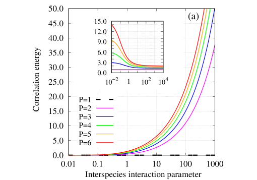
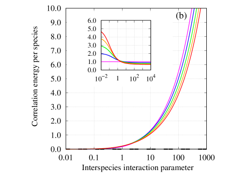
Figure 1: (a) Correlation energy, $E_{cor}$, at the infinite-particle-number limit of $P$ species of bosons as a function of the interspecies interaction parameter $\Lambda_{12}$. The intraspecies interactions are zero. The inset plots the correlation energy of a mixture with $P$ species divided by that of $P=2$ species, which we term the relative correlation energy. (b) Same as (a) but for the correlation energy per species, $\frac{E_{cor}}{P}$, at the infinite-particle-number limit. See the text for further discussion. The quantities shown are dimensionless.

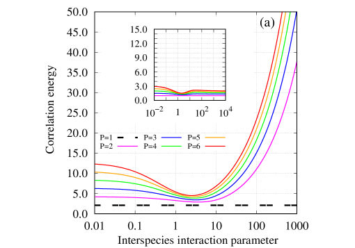
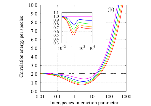
Figure 2: (a) Correlation energy, $E_{cor}$, and (b) correlation energy per particle, $\frac{E_{cor}}{P}$, at the infinite-particle-number limit of $P$ species of bosons as a function of the interspecies interaction parameter $\Lambda_{12}$. Same as Fig. 1 but when the intraspecies interactions are $\Lambda_{1}=10$. See the text for further discussion. The quantities shown are dimensionless.

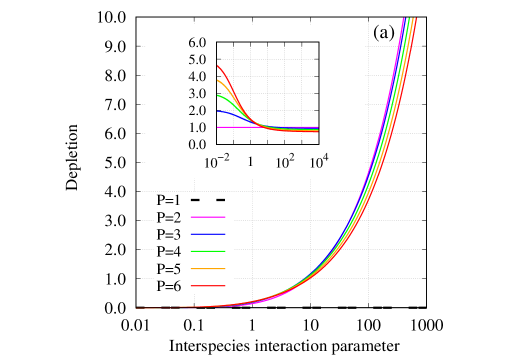
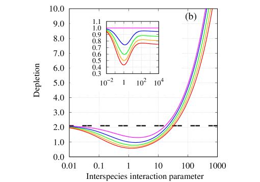
Figure 3: (a) Depletion, $d_{1}^{(1)}$, at the infinite-particle-number limit of species $1$ bosons in the $P$-species mixture as a function of the interspecies interaction parameter $\Lambda_{12}$. The inset depicts the depletion of a mixture with $P$ species divided by that of $P=2$ species, which we term the relative depletion. The intraspecies interactions are zero. (b) Same as panel (a) but when the intraspecies interactions are $\Lambda_{1}=10$. The depletion, $d_{1}^{(1)}$, and correlation energy per species, $\frac{E_{cor}}{P}$, behave similarly, compare Fig. 1b to panel (a) and Fig. 2b to panel (b), respectively. See the text for further discussion. The quantities shown are dimensionless.

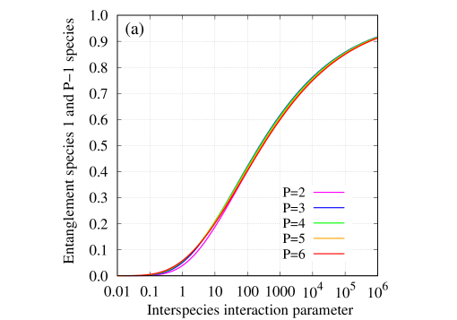
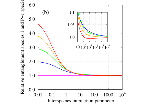
Figure 4: (a) Depicted is the Schmidt-decomposition parameter, $\rho^{2}$, defining the von Neumann entanglement entropy between one species of bosons and the other $P-1$ species at the infinite-particle-number limit as a function of the interspecies interaction parameter $\Lambda_{12}$. (b) $\rho^{2}$ in a mixture with $P$ species divided by that with $P=2$ species, which for brevity we term the relative Schmidt-decomposition parameter (relative entanglement). The inset zooms in on the results. The Schmidt-decomposition parameter, $\rho^{2}$, follows the trend of the uncertainty product, ${\Delta^{2}}_{\hat{X}_{1,CM}}{\Delta^{2}}_{\hat{P}_{X_{1,CM}}}$, compare Figs. 4 and 5. The respective functional dependence between the two quantities is given in Eq. (75). See the text for further discussion. The quantities shown are dimensionless.

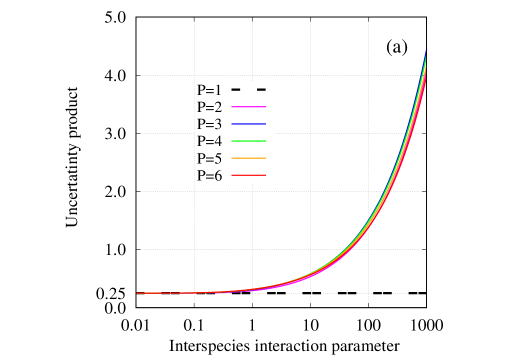
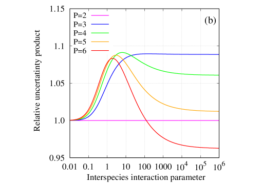
Figure 5: (a) Uncertainty product, ${\Delta^{2}}_{\hat{X}_{1,CM}}{\Delta^{2}}_{\hat{P}_{X_{1,CM}}}$, at the infinite-particle-number limit of species $1$ bosons in the $P$-species mixture as a function of the interspecies interaction parameter $\Lambda_{12}$. (b) Shown is the uncertainty product in a mixture with $P$ species divided by that with $P=2$ species, which we term the relative uncertainty product. The uncertainty product, ${\Delta^{2}}_{\hat{X}_{1,CM}}{\Delta^{2}}_{\hat{P}_{X_{1,CM}}}$, follows the trend of the Schmidt-decomposition parameter, $\rho^{2}$, compare Figs. 5 and 4. The respective functional dependence between the two quantities is given in Eq. (74). See the text for further discussion. The quantities shown are dimensionless.

V Summary and Outlook

We have presented in this work a solvable many-body model for a trapped multiple-species mixture of Bose-Einstein condensates, and, as an application, used it to construct a theory and analyze the correlation properties of $P$-species bosonic mixtures at the infinite-particle-number limit.

We first obtained closed-form expressions for various quantities as a function of the interactions and numbers of bosons. These expressions will be used in future work to investigate properties of multiple-species bosonic mixtures with a finite number of particles. The infinite-particle-number limit is then performed explicitly.

As a starter, the energy per particle, density per particle, and condensate fraction are proven to boil down in the $P$-species mixture to their mean-field counterparts. We then employ four properties to characterize correlations and investigate how they change as a function of interactions and, in particular, with the number of species in the mixture. The properties investigated are the correlation energy of the mixture, depletion of the species, the von Neumann entanglement entropy between one species and the remaining $P-1$ species, and the position–momentum uncertainty product of the species. As a general trend, correlations at the infinite-particle-number limit increase with interspecies interactions, although not monotonously if the intraspecies interactions are not zero.

The dependence of correlations at the infinite-particle-number limit on the number of species $P$ is found to be intricate. First, the behaviors of the correlation energy per species and of the depletion follow a similar trend, and, second, the entanglement entropy and uncertainty product are shown to be interconnected. Chiefly, the correlation energy per species and the depletion exhibit a crossover from weak to strong interspecies interactions with the number of species $P$ (for zero intraspecies interactions). For weak interactions, the larger is the number of species the more correlated is the mixture, whereas for strong interactions it is the other way around. Furthermore, the von Neumann entanglement entropy (Schmidt-decomposition parameter) and uncertainty product also show a crossover from weak to strong interspecies interactions. Again, for weak interactions, the larger is the number of species the more correlated is the mixture, but for strong interactions we find an optimal number of species, here $P=3$, which maximizes the correlations in the mixture. The latter represents the competition and balance between interspecies interactions and the intraspecies center-of-mass ‘weight’ as $P$ is increased.

As an outlook, we touch upon a couple of the many interesting possibilities that lie ahead. One would naturally begin with the investigation of multiple-species mixtures with finite numbers of particles. Going beyond the balanced mixture, generalizing the present treatment to the generic multiple-species mixture would be rewarding. Then, the different masses, intraspecies and interspecies interactions, and the numbers of particles of the different species is expected to enrich even more the properties of multiple-species mixtures with finite numbers of particles, as well as at the infinite-particle-number limit(s). In the latter case, e.g., some of the species could remain finite while the rest become infinite. A general question in a multiple-species mixture is how its connectivity, i.e., which species in the mixture interact with each other, dictates properties. We have seen above clues for partial insensitivity of the mean-field solution to the connectivity in the mixture, and the issue calls for further investigations. On the other end, at the many-body level of theory, the question of how entanglement between one group of non-interacting species is transfered to a second group of non-interacting species linked by a ‘bridge’ between them would be interesting to explore.

Finally, in the longer run, the present results and above prospected developments are expected to find applications in modeling Bose-Einstein condensates in cavities and benchmarking coupled-cluster theory for bosonic mixtures beyond the ‘two-species’ treatments in HIM_MIX_CC ; HIM_BEC_CAVITY , respectively. This is a good place to conclude the present work.

Appendix A Revisiting the two-species mixture and its properties at the infinite-particle-number limit

In this appendix, we revisit the two-species mixture at the infinite-particle-number limit, and collect results as far as they are needed for comparison with and exposition of the main text. To this end, we apply the elimination of the other species’ center-of-mass scheme to re-derive more concisely literature results, and to augment them with derivation of the correlation energy and the depletion.

The two-species balanced-mixture Hamiltonian is given by

$$\hat{H}({\bf x}_{1},\ldots,{\bf x}_{N},{\bf y}_{1},\ldots,{\bf y}_{N})=\sum_{j=1}^{N}\left(-\frac{1}{2}\frac{\partial^{2}}{\partial{\bf x}_{j}^{2}}+\frac{1}{2}\omega^{2}{\bf x}_{j}^{2}\right)+\sum_{j=1}^{N}\left(-\frac{1}{2}\frac{\partial^{2}}{\partial{\bf y}_{j}^{2}}+\frac{1}{2}\omega^{2}{\bf y}_{j}^{2}\right)+$$

$$+\lambda_{1}\sum_{1\leq j<k}^{N}({\bf x}_{j}-{\bf x}_{k})^{2}+\lambda_{1}\sum_{1\leq j<k}^{N}({\bf y}_{j}-{\bf y}_{k})^{2}+\lambda_{12}\sum_{j=1}^{N}\sum_{k=1}^{N}({\bf x}_{j}-{\bf y}_{k})^{2}.\$$ (78)

Introducing the Jacoby coordinates of each species

$${\bf X}_{s}=\frac{1}{\sqrt{s(s+1)}}\sum_{j=1}^{s}({\bf x}_{s+1}-{\bf x}_{j}),\ \ 1\leq s\leq N-1,\quad{\bf X}_{N}=\frac{1}{\sqrt{N}}\sum_{j=1}^{N}{\bf x}_{j},$$

$${\bf Y}_{s}=\frac{1}{\sqrt{s(s+1)}}\sum_{j=1}^{s}({\bf y}_{s+1}-{\bf y}_{j}),\ \ 1\leq s\leq N-1,\quad{\bf Y}_{N}=\frac{1}{\sqrt{N}}\sum_{j=1}^{N}{\bf y}_{j},\$$ (79)

the Hamiltonian (A) is written as a sum of two, $\hat{H}=\hat{H}_{rels}+\hat{H}_{CMs}$. The Hamiltonian of the relative motions is

$$\hat{H}_{rels}({\bf X}_{1},\ldots,{\bf X}_{N-1},{\bf Y}_{1},\ldots,{\bf Y}_{N-1})=\sum_{j=1}^{N-1}\left(-\frac{1}{2}\frac{\partial^{2}}{\partial{\bf X}_{j}^{2}}+\frac{1}{2}\Omega_{1}^{2}{\bf X}_{j}^{2}\right)+$$

$$+\sum_{j=1}^{N-1}\left(-\frac{1}{2}\frac{\partial^{2}}{\partial{\bf Y}_{j}^{2}}+\frac{1}{2}\Omega_{1}^{2}{\bf Y}_{j}^{2}\right),\$$ (80)

where

$$\Omega_{1}=\sqrt{\omega^{2}+2\left[\left(1+\frac{1}{N-1}\right)\Lambda_{1}+\Lambda_{12}\right]}.$$ (81)

The relative-motion frequency of each species, $\Omega_{1}$, is affected by the intraspecies interaction and, of course, by the interaction with the other species.

The Hamiltonian of the center-of-masses is

$$\hat{H}_{CMs}({\bf X}_{N},{\bf Y}_{N})=-\frac{1}{2}\left(\frac{\partial^{2}}{\partial{\bf X}_{N_{1}}^{2}}+\frac{\partial^{2}}{\partial{\bf Y}_{N_{2}}^{2}}\right)+\frac{1}{2}\begin{pmatrix}{\bf X}_{N}&{\bf Y}_{N}\cr\end{pmatrix}\underline{\underline{\bf O}}\begin{pmatrix}{\bf X}_{N}\cr{\bf Y}_{N}\cr\end{pmatrix},$$

$$\underline{\underline{\bf O}}=\left(\omega^{2}+4\Lambda_{12}\right)\underline{\underline{\bf I}}-2\Lambda_{12}\underline{\underline{\bf 1}}.\$$ (82)

Diagonalizing the frequencies’ matrix $\underline{\underline{\bf O}}$ one finds the two eigenvalues and eigenvectors associated with the mixture’s center-of-mass degrees-of-freedom,

$$\Omega_{12}=\sqrt{\omega^{2}+4\Lambda_{12}},\quad\omega,\$$ (83)

and

$${\bf Q}_{1}=\frac{1}{\sqrt{2}}\left(-{\bf X}_{N}+{\bf Y}_{N}\right),\qquad{\bf Q}_{2}=\frac{1}{\sqrt{2}}\left({\bf X}_{N}+{\bf Y}_{N}\right),\$$ (84)

respectively. The latter are the Jacoby coordinates built from the two center-of-mass Jacoby coordinates of the two species, ${\bf X}_{N}$ and ${\bf Y}_{N}$. Both vectors, the relative center-of-mass motion ${\bf Q}_{1}$ and the center-of-mass motion ${\bf Q}_{2}$ of the mixture do not depend on the strength of the interaction between the two species. The frequencies $\Omega_{12},\omega$ and eigenvectors ${\bf Q}_{1},{\bf Q}_{2}$ are fundamental quantities in the present appendix, and their properties for three-species and multiple-species mixtures are investigated and utilized in the main text.

The ground-state wavefunction is then a product of the relative motions and center-of-masses parts and takes on the separable form

$$\Psi({\bf X}_{1},\ldots,{\bf Y}_{1},\ldots,{\bf Q}_{1},{\bf Q}_{2})=\left(\frac{\Omega_{1}}{\pi}\right)^{\frac{3(N_{1}-1)}{2}}\left(\frac{\Omega_{12}}{\pi}\right)^{\frac{3}{4}}\left(\frac{\omega}{\pi}\right)^{\frac{3}{4}}\times$$

$$\times e^{-\frac{1}{2}\left(\Omega_{1}\sum_{k=1}^{N-1}{\bf X}_{k}^{2}+\Omega_{1}\sum_{k=1}^{N-1}{\bf Y}_{k}^{2}\right)}e^{-\frac{1}{2}\left(\Omega_{12}{\bf Q}_{1}^{2}+\omega{\bf Q}_{2}^{2}\right)}$$ (85)

along with the ground-state energy

$$\!\!\!\!\!\!\!\!\!\!\!\!E=\frac{3}{2}\left[2(N-1)\Omega_{1}+\Omega_{12}+\omega\right]=$$

$$\!\!\!\!\!\!\!\!\!\!\!\!=\frac{3}{2}\left[2(N-1)\sqrt{\omega^{2}+2\left[\left(1+\frac{1}{N-1}\right)\Lambda_{1}+\Lambda_{12}\right]}+\sqrt{\omega^{2}+4\Lambda_{12}}+\omega\right].\$$ (86)

Recall that the two frequencies must be positive for the mixture to be bound. Thus,

$$\Lambda_{12}>-\frac{\omega^{2}}{4},\qquad\Lambda_{1}>-\left(1-\frac{1}{N}\right)\left(\frac{\omega^{2}}{2}+\Lambda_{12}\right).\$$ (87)

Hence, the energy (A) is bound from below but not from above.

To proceed, we work in the representation of the wavefunction using explicitly the Jacoby coordinates of each species,

$$\Psi({\bf X}_{1},\ldots,{\bf X}_{N},{\bf Y}_{1},\ldots,{\bf Y}_{N})=\left(\frac{\Omega_{1}}{\pi}\right)^{\frac{3(N-1)}{2}}\left(\frac{\Omega_{12}}{\pi}\right)^{\frac{3}{4}}\left(\frac{\omega}{\pi}\right)^{\frac{3}{4}}\times$$

$$\times e^{-\frac{1}{2}\Omega_{1}\sum_{k=1}^{N-1}{\bf X}_{k}^{2}}e^{-\frac{1}{2}\Omega_{1}\sum_{k=1}^{N-1}{\bf Y}_{k}^{2}}e^{-\frac{1}{2}a{\bf X}_{N}^{2}}e^{-\frac{1}{2}a{\bf Y}_{N}^{2}}e^{-b{\bf X}_{N}{\bf Y}_{N}},\$$ (88)

where

$$a=\frac{1}{2}\left(\Omega_{12}+\omega\right)=\Omega_{12}+b,\qquad b=\frac{1}{2}\left(\omega-\Omega_{12}\right).\$$ (89)

The coefficients are interrelated and satisfy $a+b=\omega$. Their scaling properties at the limit of an infinite number of particles are discussed below, and their generalizations to more species have been presented in the main text.

Then, the all-particle density matrix expressed using the species’ Jacoby coordinates is

$$\Psi({\bf X}_{1},\ldots,{\bf X}_{N},{\bf Y}_{1},\ldots,{\bf Y}_{N})\Psi^{\ast}({\bf X}^{\prime}_{1},\ldots,{\bf X}^{\prime}_{N},{\bf Y}^{\prime}_{1},\ldots,{\bf Y}^{\prime}_{N})=$$

$$=\left(\frac{\Omega_{1}}{\pi}\right)^{3(N-1)}\left(\frac{\Omega_{12}}{\pi}\right)^{\frac{3}{2}}\left(\frac{\omega}{\pi}\right)^{\frac{3}{2}}e^{-\frac{1}{2}\Omega_{1}\sum_{k=1}^{N-1}\left({\bf X}_{k}^{2}+{{\bf X}^{\prime}}_{k}^{2}\right)}e^{-\frac{1}{2}\Omega_{1}\sum_{k=1}^{N-1}\left({\bf Y}_{k}^{2}+{{\bf Y}^{\prime}}_{k}^{2}\right)}\times$$

$$\times e^{-\frac{1}{2}a\left({\bf X}_{N}^{2}+{{\bf X}^{\prime}}_{N}^{2}\right)}e^{-\frac{1}{2}a\left({\bf Y}_{N}^{2}+{{\bf Y}^{\prime}}_{N}^{2}\right)}e^{-b\left({\bf X}_{N}{\bf Y}_{N}+{\bf X}^{\prime}_{N}{\bf Y}^{\prime}_{N}\right)}.\$$ (90)

Upon substitution of $a$ and $b$, and translating from Jacoby coordinates to the laboratory frame, the all-particle density matrix in HIM_MIX_RDM , when considering a balanced mixture Atoms_2021 , is recovered.

The integration of (A) to arrive at the intraspecies reduced density matrices of species $1$ bosons is performed in a few steps. The first is eliminating the relative coordinates of species $2$ $\{{\bf Y}^{\prime}_{k}={\bf Y}_{k},k=1,\ldots,N-1\}$. The second step is integrating over the center-of-mass coordinate of species $2$ ${\bf Y}^{\prime}_{N}={\bf Y}_{N}$, i.e.,

$$\int d{\bf Y}_{N}e^{-a{\bf Y}_{N}^{2}}e^{-b\left({\bf X}_{N}+{\bf X}^{\prime}_{N}\right){\bf Y}_{N}}=\left(\frac{\pi}{a}\right)^{\frac{3}{2}}e^{+\frac{1}{4}\frac{b^{2}}{a}\left({\bf X}_{N}+{\bf X}^{\prime}_{N}\right)^{2}}.\$$ (91)

With this, all dependencies on the coordinates of species $2$ have been integrated out. Translating the result from the Jacoby coordinates to the laboratory frame we arrive at the working expression

$$e^{-\frac{\alpha}{2}\sum_{j=1}^{N}\left({\bf x}_{j}^{2}+{{\bf x}^{\prime}}_{j}^{2}\right)-\beta\sum_{1\leq j<k}^{N}\left({\bf x}_{j}{\bf x}_{k}+{\bf x}^{\prime}_{j}{\bf x}^{\prime}_{k}\right)}e^{-\frac{1}{4}C_{N,0}\left\{\sum_{j=1}^{N}\left({\bf x}_{j}+{\bf x}^{\prime}_{j}\right)\right\}^{2}},\$$ (92)

in which all the information on the interaction with species $2$ is contained in the three coefficients,

$$\alpha=\Omega_{1}+\frac{1}{N}\left(a-\Omega_{1}\right)=\Omega_{1}\left\{1+\frac{1}{N}\left[\frac{1}{2}\left(\frac{\omega}{\Omega_{1}}+\frac{\Omega_{12}}{\Omega_{1}}\right)-1\right]\right\},$$

$$\beta=\alpha-\Omega_{1}=\Omega_{1}\frac{1}{N}\left[\frac{1}{2}\left(\frac{\omega}{\Omega_{1}}+\frac{\Omega_{12}}{\Omega_{1}}\right)-1\right],$$

$$C_{N,0}=-\frac{1}{N}\frac{b^{2}}{a}=-\frac{1}{N}\frac{1}{2}\frac{\left(\omega-\Omega_{12}\right)^{2}}{\left(\omega+\Omega_{12}\right)},$$ (93)

where the following relation has been used $\sum_{s=1}^{N-1}{\bf X}_{s}^{2}=\left(1-\frac{1}{N}\right)\sum_{j=1}^{N}{\bf x}_{j}^{2}-\frac{2}{N}\sum_{1\leq j<k}^{N}{\bf x}_{j}{\bf x}_{k}$. $C_{N,0}$, as should be expected, is precisely the expression obtained in HIM_MIX_RDM , when taking the balanced mixture, which now allows one for intraspecies integration of (92) following HIM_Cohen .

The reduced one-particle density matrix then reads

$$\rho^{(1)}_{1}({\bf x},{\bf x}^{\prime})=N\left(\frac{\alpha+C_{1,0}}{\pi}\right)^{\frac{3}{2}}e^{-\frac{\alpha}{2}\left({\bf x}^{2}+{{\bf x}^{\prime}}^{2}\right)}e^{-\frac{1}{4}C_{1,0}\left({\bf x}+{\bf x}^{\prime}\right)^{2}},$$ (94)

$$\rho^{(1)}_{1}({\bf x})=N\left(\frac{\alpha+C_{1,0}}{\pi}\right)^{\frac{3}{2}}e^{-\left(\alpha+C_{1,0}\right){\bf x}^{2}},\$$

with

$$\!\!\!\!\!\!\!\!\!\!\!\!\!\!\!\!\alpha+C_{1,0}=\left(\alpha-\beta\right)\frac{\left(\alpha-\beta\right)+N\left(C_{N,0}+\beta\right)}{\left(\alpha-\beta\right)+(N-1)\left(C_{N,0}+\beta\right)}=\Omega_{1}\frac{1}{1+\frac{1}{N}\left[\frac{1}{2}\left(\frac{\Omega_{1}}{\omega}+\frac{\Omega_{1}}{\Omega_{12}}\right)-1\right]},\$$ (95)

where $C_{N,0}+\beta=C_{N,0}+\alpha-\Omega_{1}=\frac{1}{N}\left(\frac{2\omega\Omega_{12}}{\omega+\Omega_{12}}-\Omega_{1}\right)=-\frac{2\omega\Omega_{12}}{\omega+\Omega_{12}}\frac{1}{N}\left[\frac{1}{2}\left(\frac{\Omega_{1}}{\omega}+\frac{\Omega_{1}}{\Omega_{12}}\right)-1\right]$ and $C_{N,0}+\alpha=\Omega_{1}\left(1-\frac{1}{N}\right)+\frac{1}{N}\left(\frac{a^{2}-b^{2}}{a}\right)=\Omega_{1}\left(1-\frac{1}{N}\right)+\frac{1}{N}\left(\frac{2\omega\Omega_{12}}{\omega+\Omega_{12}}\right)$ are used.

The essence of the mean-field solution goes as follows. The detailed derivation is given in HIM_MIX_RDM . The ansatz for the wavefunction is the separable product state

$$\Phi^{GP}({\bf x}_{1},\ldots,{\bf x}_{N},{\bf y}_{1},\ldots,{\bf y}_{N})=\prod_{j=1}^{N}\phi^{GP}_{1}({\bf x}_{j})\prod_{k=1}^{N}\phi^{GP}_{2}({\bf y}_{k}).$$ (96)

Sandwiching the many-body Hamiltonian and using the variational principle, the coupled Gross-Pitaevskii equations are obtained, and their solution is given by

$$\phi^{GP}_{1}({\bf x})=\left(\frac{\Omega_{1}^{GP}}{\pi}\right)^{\frac{3}{4}}e^{-\frac{1}{2}\Omega_{1}^{GP}{\bf x}^{2}},\quad\Omega_{1}^{GP}=\sqrt{\omega^{2}+2\left(\Lambda_{1}+\Lambda_{12}\right)},$$

$$\phi^{GP}_{2}({\bf y})=\left(\frac{\Omega_{1}^{GP}}{\pi}\right)^{\frac{3}{4}}e^{-\frac{1}{2}\Omega_{1}^{GP}{\bf y}^{2}}.\$$ (97)

The two orbitals are the same in the balanced system. There is no demixing in this model, also see HIM_MIX_RDM . We mention in this context that a modification of the harmonic-interaction model to emulate demixing of two Bose-Einstein condensates is introduced and used in HIM_JPCS_2022 . The chemical potentials are $\mu_{1}=\mu_{2}=\frac{3}{2}\left(\Omega_{1}^{GP}+\frac{\Lambda_{1}+\Lambda_{12}}{\Omega_{1}^{GP}}\right)$. The Gross-Pitaevskii energy per particle can be written as

$$\varepsilon^{GP}=\frac{E^{GP}}{2N}=\frac{3}{2}\Omega_{1}^{GP}=\frac{3}{2}\sqrt{\omega^{2}+2\left(\Lambda_{1}+\Lambda_{12}\right)}.$$ (98)

That the infinite-particle-number limit implies $100\%$ Bose-Einstein condensation and boiling down to the mean-field quantities is shown now.

Thus, one finds for the energy of the mixture at the infinite-particle-number limit

$$\lim_{N\to\infty\atop J=1,2}\frac{E}{2N}=\varepsilon^{GP},$$ (99)

and for the reduced one-particle density matrix of species $1$

$$\!\!\!\!\!\!\!\!\!\!\!\!\lim_{N\to\infty\atop J=1,2}\frac{\rho^{(1)}_{1}({\bf x},{\bf x}^{\prime})}{N}=\phi^{GP}_{1}({\bf x})\left\{\phi^{GP}_{1}({\bf x}^{\prime})\right\}^{\ast}.$$ (100)

Clearly from (100), also the density per particle, which is the diagonal of the reduced one-particle density matrix, $\rho^{(1)}_{1}({\bf x})\equiv\rho^{(1)}_{1}({\bf x},{\bf x}^{\prime}={\bf x})$, per particle, boils down to the respective mean-field density. Finally, since the mixture is balanced per consideration, or, alternatively, the assignment of the labeling $1$ and $2$ to the species is arbitrary, relation (100) holds for species $2$ in the mixture as well.

Next, the correlation energy reads

$$\!\!\!\!\!\!\!\!\!\!\!\!\!\!\!\!\!\!\!\!E_{cor}=E^{GP}-E=\frac{3}{2}\Bigg{[}2N\sqrt{\omega^{2}+2\left(\Lambda_{1}+\Lambda_{12}\right)}-$$

$$\!\!\!\!\!\!\!\!\!\!\!\!\!\!\!\!\!\!\!\!-2(N-1)\sqrt{\omega^{2}+2\left[\left(1+\frac{1}{N-1}\right)\Lambda_{1}+\Lambda_{12}\right]}-\sqrt{\omega^{2}+4\Lambda_{12}}-\omega\Bigg{]}.\$$ (101)

Using $\Omega_{1}=\sqrt{\omega^{2}+2\left[\left(1+\frac{1}{N-1}\right)\Lambda_{1}+\Lambda_{12}\right]}=\Omega_{1}^{GP}\sqrt{1+\frac{2\Lambda_{1}}{(N-1)\{\Omega_{1}^{GP}\}^{2}}}$ one obtains at the infinite-particle-number limit

$$\!\!\!\!\!\!\!\!\lim_{N\to\infty\atop J=1,2}E_{cor}=\frac{3}{2}\Bigg{[}2\sqrt{\omega^{2}+2\left(\Lambda_{1}+\Lambda_{12}\right)}-\frac{2\Lambda_{1}}{\sqrt{\omega^{2}+2\left(\Lambda_{1}+\Lambda_{12}\right)}}-\sqrt{\omega^{2}+4\Lambda_{12}}-\omega\Bigg{]}=$$

$$=\frac{3}{2}\left[2\Omega_{1}^{GP}-\frac{2\Lambda_{1}}{\Omega_{1}^{GP}}-\Omega_{123}-\omega\right].\$$ (102)

Expression (A) tells us that, even at the limit of an infinite number of particles when the two species are 100% condensed and the many-body and mean-field energies per particle coincide, there are correlations in the mixture.

The reduced one-particle density matrix (94,95) is diagonalized using Meheler’s formula Robinson_1977 ; Schilling_2013 ; Atoms_2021 . From which, the final result for the depletion of species $1$ reads

$$d^{(1)}_{1}=N\left[1-\left(1-\rho^{(1)}_{1}\right)^{3}\right]=N\rho^{(1)}_{1}\left(3-3\rho^{(1)}_{1}+\left\{\rho^{(1)}_{1}\right\}^{2}\right),$$

$$\rho^{(1)}_{1}=\frac{\mathcal{W}-1}{\mathcal{W}+1},\qquad\qquad\mathcal{W}=\sqrt{\frac{\alpha}{\alpha+C_{1,0}}}=$$ (103)

$$=\sqrt{\left\{1+\frac{1}{N}\left[\frac{1}{2}\left(\frac{\omega}{\Omega_{1}}+\frac{\Omega_{12}}{\Omega_{1}}\right)-1\right]\right\}\left\{1+\frac{1}{N}\left[\frac{1}{2}\left(\frac{\Omega_{1}}{\omega}+\frac{\Omega_{1}}{\Omega_{12}}\right)-1\right]\right\}}.\$$

At the infinite-particle-number limit we obtain the depletion

$$\lim_{N\to\infty\atop J=1,2}d^{(1)}_{1}=\frac{3}{4}\left[\frac{1}{2}\frac{\left(\omega-\Omega_{1}^{GP}\right)^{2}}{\omega\Omega_{1}^{GP}}+\frac{1}{2}\frac{\left(\Omega_{12}-\Omega_{1}^{GP}\right)^{2}}{\Omega_{12}\Omega_{1}^{GP}}\right].\$$ (104)

In the absence of interaction between the two species, (104) reduces to the single-species infinite-particle-number depletion, see INF_LENZ_2017 .

The Schmidt decomposition of the wavefunction (A) goes as follows, also see Atoms_2021 . Since the Jacoby relative coordinates’ parts of the wavefunction are separable, we only need to Schmidt decompose the parts with the coupled intraspecies center-of-mass Jacoby coordinates. We dub these parts of the wavefunction as the mixture’s normalized center-of-masses wavefunction. It is given along with the final result of the decomposition by

$$\Psi_{CMs}({\bf X}_{N},{\bf Y}_{N})=\left(\frac{a^{2}-b^{2}}{\pi^{2}}\right)^{\frac{3}{4}}e^{-\frac{1}{2}a\left({\bf X}^{2}_{N}+{\bf Y}^{2}_{N}\right)}e^{-b{\bf X}_{N}{\bf Y}_{N}}=$$

$$=\sum_{n_{1},n_{2},n_{3}=0}^{\infty}\left(1-\rho^{2}\right)^{\frac{3}{2}}\rho^{n_{1}+n_{2}+n_{3}}\Phi_{n_{1},n_{2},n_{3}}({\bf X}_{N};s)\Phi_{n_{1},n_{2},n_{3}}({\bf Y}_{N};s),\$$ (105)

where

$$\!\!\!\!\!\!\!\!\!\!\!\!\!\!\!\!\!\!\!\!s=\sqrt{a^{2}-b^{2}}=\sqrt{\Omega_{12}\omega},\qquad\rho=\frac{\mathcal{W}_{SD}-1}{\mathcal{W}_{SD}+1},\qquad\mathcal{W}_{SD}=\sqrt{\frac{a-b}{a+b}}=\sqrt{\frac{\Omega_{12}}{\omega}},\$$ (106)

which holds for attractive interspecies interaction ($b<0$). For repulsive interspecies interaction ($b>0$), just take, say, ${\bf Y}_{N}\to-{\bf Y}_{N}$ in (A) and $\rho\to-\rho$ in (106).

Manifestation of that in an observable is, for instance, the position–momentum uncertainty product, i.e., deviations from the mean-field separable-solution result reflect the entanglement between the two species. Inverting (84) one computes ${\Delta^{2}}_{\hat{\bf X}_{N}}=\frac{1}{4}\left(\frac{1}{\Omega_{12}}+\frac{1}{\omega}\right)\!\mbox{\boldmath$1$}$ and ${\Delta^{2}}_{\hat{\bf P}_{{\bf X}_{N}}}=\frac{1}{4}\left(\Omega_{12}+\omega\right)\!\mbox{\boldmath$1$}$ and consequently HIM_MIX_CP

$${\Delta^{2}}_{\hat{\bf X}_{CM}}{\Delta^{2}}_{\hat{\bf P}_{{\bf X}_{CM}}}={\Delta^{2}}_{\hat{\bf X}_{N}}{\Delta^{2}}_{\hat{\bf P}_{{\bf X}_{N}}}=\left[1+\frac{1}{4}\frac{\left(\omega-\Omega_{12}\right)^{2}}{\omega\Omega_{12}}\right]\frac{1}{4}\mbox{\boldmath$1$}.$$ (107)

Indeed, the many-body result for the uncertainty product (107) reflects the entanglement between the two species, see (106). Both are a consequence of the coupling between the species center-of-masses, see (A), which survives the infinite-particle-number limit. Inversely, the coupling between the center-of-masses does not exist at the Gross-Pitaevskii level, there is no entanglement between the two species, and, consequently, $\left\{{\Delta^{2}}_{\hat{\bf X}_{CM}}{\Delta^{2}}_{\hat{\bf P}_{{\bf X}_{CM}}}\right\}^{GP}=\frac{1}{4}\mbox{\boldmath$1$}$. Further discussion is provided in Sec. III of the main text.

Appendix B Folding $P-1$ center-of-mass coordinates in the $P$-species mixture

For $P=1$ species, there are obviously no other species to fold down. Consequently,

$$C_{N}=0,\$$ (108)

which appears in the single-species treatment HIM_Cohen . For $P=2$ species one gets

$$C_{N,0}=-\frac{1}{N}\frac{b^{2}}{a},$$ (109)

see HIM_MIX_RDM and (A) in the previous appendix. For $P=3$ species we found

$$C_{N,0,0}=-\frac{1}{N}\left[\frac{b^{2}}{a}+\frac{\left(b-\frac{b^{2}}{a}\right)^{2}}{a-\frac{b^{2}}{a}}\right]=-\frac{1}{N}\frac{2b^{2}}{a+b},$$ (110)

see (II). For $P=4$ species, a concrete calculation gives

$$\!\!\!\!\!\!\!\!\!\!\!\!C_{N,0,0,0}=-\frac{1}{N}\left\{\frac{b^{2}}{a}+\frac{\left(b-\frac{b^{2}}{a}\right)^{2}}{a-\frac{b^{2}}{a}}+\frac{\left[\left(b-\frac{b^{2}}{a}\right)-\frac{\left(b-\frac{b^{2}}{a}\right)^{2}}{a-\frac{b^{2}}{a}}\right]^{2}}{\left(a-\frac{b^{2}}{a}\right)-\frac{\left(b-\frac{b^{2}}{a}\right)^{2}}{a-\frac{b^{2}}{a}}}\right\}=-\frac{1}{N}\frac{3b^{2}}{a+2b},$$ (111)

and so on. We can prove the general expression (50) using mathematical induction.

For this, we write

$$\!\!\!\!\!\!\!\!\!\!\!\!C_{N,0,\ldots,0}=-\frac{1}{N}D_{P}(a,b),\qquad D_{P}(a,b)=\sum_{p=1}^{P}d_{p}(a,b),\qquad P\geq 1,$$

$$\!\!\!\!\!\!\!\!\!\!\!\!d_{1}(a,b)=0,\quad d_{2}(a,b)=\frac{b^{2}}{a},\quad d_{p+1}(a,b)=d_{p}\left(a-\frac{b^{2}}{a},b-\frac{b^{2}}{a}\right),\ p\geq 2.\$$ (112)

Following (108,109,110,111) assume that

$$D_{P}(a,b)=\frac{(P-1)b^{2}}{a+(P-2)b}.$$ (113)

Then, one must prove using (B,113) that the succeeding relation holds

$$\!\!\!\!\!\!\!\!\!\!\!\!\!\!\!\!\!\!\!\!D_{P+1}(a,b)=D_{P}(a,b)+d_{P+1}(a,b)=D_{P}(a,b)+d_{P}\left(a-\frac{b^{2}}{a},b-\frac{b^{2}}{a}\right)=$$

$$\!\!\!\!\!\!\!\!\!\!\!\!\!\!\!\!\!\!\!\!=D_{P}(a,b)+D_{P}\left(a-\frac{b^{2}}{a},b-\frac{b^{2}}{a}\right)-D_{P-1}\left(a-\frac{b^{2}}{a},b-\frac{b^{2}}{a}\right)=\frac{Pb^{2}}{a+(P-1)b}.$$ (114)

Indeed, after some straightforward and not too lengthy algebra, Eq. (B) is readily proved for $P\geq 2$. For $P=1$ we have a single species, not a mixture, yet the general expression (113) holds as well, i.e., it reduces to (108).

References

(1)
(2) W. E. Keller, Helium-3 and Helium-4 (Springer, New York, 1969).
(3) B. H. Wiik and G. Wolf, Electron-Positron Interactions (Springer, Heidelberg, 1979).
(4) P. Ring and P. Schuck, The Nuclear many-body problem (Springer, Berlin, 1980).
(5) M. S. Dresselhaus, G. Dresselhaus, and P. Avouris (Eds.), Carbon nanotubes (Springer, Heidelberg, 2001).
(6) F. Dalfovo, S. Giorgini, L. P. Pitaevskii, and S. Stringari,
Theory of Bose-Einstein condensation in trapped gases,
Rev. Mod. Phys. 71, 463 (1999).
(7) A. J. Leggett,
Bose-Einstein condensation in the alkali gases: Some fundamental concepts,
Rev. Mod. Phys. 73, 307 (2001).
(8) I. Bloch, J. Dalibard, and W. Zwerger,
Many-body physics with ultracold gases,
Rev. Mod. Phys. 80, 885 (2008).
(9) D. C. Roberts and M. Ueda,
Stability analysis for -component Bose-Einstein condensate,
Phys. Rev. A 73, 053611 (2006).
(10) P. Mason and S. A. Gardiner,
Number-conserving approaches to -component Bose-Einstein condensates,
Phys. Rev. A 89, 043617 (2014).
(11) A. Barman and S. Basu,
Phase diagram of multi-component bosonic mixtures: emergence of mixed superfluid and insulating phases,
J. Phys. B 48, 055301 (2015).
(12) Y. Eto, M. Takahashi, K. Nabeta, R. Okada, M. Kunimi, H. Saito, and T. Hirano,
Bouncing motion and penetration dynamics in multicomponent Bose-Einstein condensates,
Phys. Rev. A 93, 033615 (2016).
(13) Y. Z. He, Y. M. Liu, and C. G. Bao,
Spin-structures of the Bose-Einstein condensates with three kinds of spin-1 atoms,
Sci. Rep. 10, 2727 (2020).
(14) K. Jimbo and H. Saito,
Surfactant behavior in three-component Bose-Einstein condensates,
Phys. Rev. A 103, 063323 (2021).
(15) Y. Ma, C. Peng, and X. Cui,
Borromean Droplet in Three-Component Ultracold Bose Gases,
Phys. Rev. Lett. 127, 043002 (2021).
(16) C. Liu, P. Chen, L. He, and F. Xu,
Ground-state properties of multicomponent bosonic mixtures: A Gutzwiller mean-field study,
Phys. Rev. A 108, 013309 (2023).
(17) A. Saboo, S. Halder, S. Das, and S. Majumder,
Rayleigh-Taylor instability in a phase-separated three-component Bose-Einstein condensate,
Phys. Rev. A 108, 013320 (2023).
(18) Y. Ma, T.-L. Ho, and X. Cui,
Shell-shaped quantum droplet in a three-component ultracold Bose gas,
arXiv:2312.15846v1 [cond-mat.quant-gas].
(19) S. Pruski, J. Maćkowiak, and O. Missuno,
Reduced density matrices of a system of coupled oscillators. 2.
Eigenstructure of the -particle matrix for the canonical ensemble,
Rep. Math. Phys. 3, 227 (1972).
(20) S. Pruski, J. Maćkowiak, and O. Missuno,
Reduced density matrices of a system of coupled oscillators. 3.
The eigenstructure of the -particle matrix for the ground state,
Rep. Math. Phys. 3, 241 (1972).
(21) P. D. Robinson,
Coupled oscillator natural orbitals,
J. Chem. Phys. 66, 3307 (1977).
(22) R. L. Hall,
Some exact solutions to the translation-invariant -body problem,
J. Phys. A 11, 1227 (1978).
(23) R. L. Hall,
Exact solutions of Schrödinger’s equation for translation-invariant harmonic matter,
J. Phys. A 11, 1235 (1978).
(24) L. Cohen and C. Lee,
Exact reduced density matrices for a model problem,
J. Math. Phys. 26, 3105 (1985).
(25) M. S. Osadchii and V. V. Muraktanov,
The System of Harmonically Interacting Particles:
An Exact Solution of the Quantum-Mechanical Problem,
Int. J. Quant. Chem. 39, 173 (1991).
(26) M. A. Załuska-Kotur, M. Gajda, A. Orłowski, and J. Mostowski,
Soluble model of many interacting quantum particles in a trap,
Phys. Rev. A 61, 033613 (2000).
(27) J. Yan,
Harmonic Interaction Model and Its Applications in Bose-Einstein Condensation,
J. Stat. Phys. 113, 623 (2003).
(28) M. Gajda,
Criterion for Bose-Einstein condensation in a harmonic
trap in the case with attractive interactions,
Phys. Rev. A 73, 023603 (2006).
(29) J. R. Armstrong, N. T. Zinner, D. V. Fedorov, and A. S. Jensen,
Analytic harmonic approach to the -body problem,
J. Phys. B 44 055303, (2011).
(30) J. R. Armstrong, N. T. Zinner, D. V. Fedorov, and A. S. Jensen,
Virial expansion coefficients in the harmonic approximation,
Phys. Rev. E 86, 021115 (2012).
(31) P. Kościk and A. Okopińska,
Correlation effects in the Moshinsky model,
Few-Body Syst. 54, 1637 (2013).
(32) C. Schilling,
Natural orbitals and occupation numbers for harmonium: Fermions versus bosons,
Phys. Rev. A 88, 042105 (2013).
(33) P. A. Bouvrie, A. P. Majtey, M. C. Tichy, J. S. Dehesa, and A. R. Plastino,
Entanglement and the Born-Oppenheimer approximation
in an exactly solvable quantum many-body system,
Eur. Phys. J. D 68, 346 (2014).
(34) C. L. Benavides-Riveros, I. V. Toranzo, and J. S. Dehesa,
Entanglement in N-harmonium: bosons and fermions,
J. Phys. B 47, 195503 (2014).
(35) J. R. Armstrong, A. G. Volosniev, D. V. Fedorov, A. S. Jensen, and N. T. Zinner,
Analytic solutions of topologically disjoint systems,
J. Phys. A 48, 085301 (2015).
(36) C. Schilling and R. Schilling,
Number-parity effect for confined fermions in one dimension,
Phys. Rev. A 93, 021601(R) (2016).
(37) O. E. Alon,
Solvable model of a generic trapped mixture of interacting bosons:
reduced density matrices and proof of Bose-Einstein condensation,
J. Phys. A 50, 295002 (2017).
(38) O. E. Alon and L. S. Cederbaum,
Entanglement and correlations in an exactly-solvable model of a Bose-Einstein condensate in a cavity,
J. Phys. A 57, 295305 (2024).
(39) E. H. Lieb, R. Seiringer, and J. Yngvason,
Bosons in a trap: A rigorous derivation of the Gross-Pitaevskii energy functional,
Phys. Rev. A 61, 043602 (2000).
(40) E. H. Lieb and R. Seiringer,
Proof of Bose-Einstein Condensation for Dilute Trapped Gases,
Phys. Rev. Lett. 88, 170409 (2002).
(41) Y. Castin and R. Dum,
Low-temperature Bose-Einstein condensates in time-dependent traps: Beyond the symmetry-breaking approach,
Phys. Rev. A 57, 3008 (1998).
(42) L. S. Cederbaum,
Exact many-body wave function and properties
of trapped bosons in the infinite-particle limit,
Phys. Rev. A 96, 013615 (2017).
(43) S. Klaiman and O. E. Alon,
Variance as a sensitive probe of correlations,
Phys. Rev. A 91, 063613 (2015).
(44) K. Sakmann and J. Schmiedmayer,
Conserving symmetries in Bose-Einstein condensate dynamics requires many-body theory,
arXiv:1802.03746v2 [cond-mat.quant-gas].
(45) S Klaiman and L. S. Cederbaum,
Overlap of exact and Gross-Pitaevskii wave functions in Bose-Einstein condensates of dilute gases,
Phys. Rev. A 94, 063648 (2016).
(46) I. Anapolitanos, M. Hott, and D. Hundertmark,
Derivation of the Hartree equation for compound Bose gases in the mean field limit,
Rev. Math. Phys. 29, 1750022 (2017).
(47) A. Michelangeli and A. Olgiati,
Mean-field quantum dynamics for a mixture of Bose-Einstein condensates,
Anal. Math. Phys. 7, 377 (2017).
(48) A. Michelangeli, P. T. Nam, and A. Olgiati,
Ground state energy of mixture of Bose gases,
Rev. Math. Phys. 31, 1950005 (2019).
(49) J. Lee,
Rate of convergence toward Hartree type equations for mixture condensates with factorized initial data,
J. Math. Phys. 62, 091901 (2021).
(50) S. Klaiman, A. I. Streltsov, and O. E. Alon,
Solvable model of a trapped mixture of Bose-Einstein condensates,
Chem. Phys. 482, 362 (2017).
(51) O. E. Alon,
Fragmentation of Identical and Distinguishable Bosons’ Pairs and Natural Geminals of a Trapped Bosonic Mixture,
Atoms 9, 92 (2021).
(52) O. E. Alon,
Solvable Model of a Generic Driven Mixture of Trapped Bose-Einstein Condensates and
Properties of a Many-Boson Floquet State at the Limit of an Infinite Number of Particles,
Entropy 22, 1342 (2020).
(53) O. E. Alon and L. S. Cederbaum,
Effects Beyond Center-of-Mass Separability in a Trapped Bosonic Mixture: Exact Results,
J. Phys.: Conf. Ser. 2249, 012011 (2022).
(54) A. Bhowmik and O. E. Alon,
Coupled-cluster theory for trapped bosonic mixtures,
J. Chem. Phys. 160, 044105 (2024).