Information criteria for the number of
directions of extremes in high-dimensional data

Abstract

In multivariate extreme value analysis, the estimation of the dependence structure in extremes is a challenging task, especially in the context of high-dimensional data. Therefore, a common approach is to reduce the model dimension by considering only the directions in which extreme values occur. In this paper, we use the concept of sparse regular variation recently introduced by meyer_sparse to derive information criteria for the number of directions in which extreme events occur, such as a Bayesian information criterion (BIC), a mean-squared error-based information criterion (MSEIC), and a quasi-Akaike information criterion (QAIC) based on the Gaussian likelihood function. As is typical in extreme value analysis, a challenging task is the choice of the number $k_{n}$ of observations used for the estimation. Therefore, for all information criteria, we present a two-step procedure to estimate both the number of directions of extremes and an optimal choice of $k_{n}$. We prove that the AIC of meyer_muscle23 and the MSEIC are inconsistent information criteria for the number of extreme directions whereas the BIC and the QAIC are consistent information criteria. Finally, the performance of the different information criteria is compared in a simulation study and applied on wind speed data.

and

1 Introduction

Multivariate extreme value statistics analyses the probabilities of joint extreme events in multivariate data with a wide range of applications, such as finance, insurance, meteorology, hydrology and, more generally, environmental risks due to the influence of climate change. This is a challenging task, especially for high-dimensional data, where modern research combines knowledge from extreme value theory with multivariate statistics and machine learning.

Multivariate regular variation is a classical concept for modeling multivariate extremes (resnick1987, resnick2007, Falk:Buch). Suppose $\boldsymbol{X}\in\mathbb{R}^{d}_{+}$ is a $d$-dimensional random vector and there exists an index $\alpha>0$ (tail index) and a measure $S$ on the unit sphere $\mathbb{S}^{d-1}_{+}\coloneqq\{\boldsymbol{x}\in\mathbb{R}^{d}_{+}:\ \|\boldsymbol{x}\|=1\}$ (spectral measure) such that

$$\mathbb{P}\left(\frac{\lVert\boldsymbol{X}\rVert}{t}>r,\frac{\boldsymbol{X}}{\lVert\boldsymbol{X}\rVert}\in A\Big{|}\,\lVert\boldsymbol{X}\rVert>t\right)\longrightarrow r^{-\alpha}S(A),\quad t\rightarrow\infty,$$ (1.1)

for all $r>0$ and all Borel sets $A\subset\mathbb{S}^{d-1}_{+}$ with $S(\partial A)=0$, then $\boldsymbol{X}$ is called multivariate regularly varying of index $\alpha$. The spectral measure $S$ contains the information about the dependence structure in the extremes of $\boldsymbol{X}$ and therefore a particular goal is the determination of $S$. However, in high-dimensional data sets where $d$ is large, this can be challenging and computationally intensive because the dependence structure in the extremes is usually complex. In the case of high dimensions, the spectral measure is often sparse and has support in a lower-dimensional subspace. Therefore, a standard approach from multivariate statistics is to first apply a dimension reduction method to find the support of $S$ and then to estimate $S$, which drastically reduces the computational time and the quality of the estimation.

The literature on dimension reduction methods for multivariate extremes using statistical learning methods has grown rapidly in recent years. Starting with chautru who first applies a principal component analysis (PCA) and then a cluster analysis with spherical $k$-means to the spectral measure of a multivariate regularly varying random vector to find a group of variables that are jointly extreme. The reconstruction error of PCA is then analyzed in DS:21 and recently, Sabourin_et_al_2024 extend the PCA approach to Hibert-valued regularly varying random objects, whereas AMDS:22 use with kernel PCA a nonlinear generalization of PCA. In addition, CT:19, MR4582715 apply a PCA to the tail pairwise dependence matrix. The unsupervised learning approach of using spherical $k$-means, a variant of $k$-means, for cluster analysis in extreme observations was taken up in AMDS:24, Bernard_2013, JW:20, Fomichov:Ivanovs. The topic of this paper is support identification of the spectral measure, related literature on support identification is damex, tawn, meyer_muscle23, pmlr-v139-jalalzai21a. A completely different line of research to represent the sparsity structure in multivariate models are graphical models as, e.g., Engelke:Hitz, Engelke:Volgushev, engelke2024, Gissibl_et_al, Gissibl_et_al:2018, to name only a few. A very nice overview of recent advances in probabilistic and statistical aspects of sparse structures in extremes is given in Engelke:Ivanovs.

The support of $S$ can be identified by the disjoint partition of the unit sphere $\mathbb{S}^{d-1}_{+}$ into sets of the form

$$C_{\beta}\coloneqq\{\boldsymbol{x}\in\mathbb{S}^{d-1}_{+}:x_{i}>0\,\text{ for }\,i\in\beta,x_{i}=0\,\text{ for }\,i\notin\beta\}\subseteq\mathbb{S}^{d-1}_{+},\quad\beta\subset\{1,\ldots,d\}.$$ (1.2)

Knowing $S(C_{\beta})$ for all $\beta\subseteq\{1,\ldots,d\}$ allows us to draw conclusions about the support of $S$ and the directions of the extremes. Of course, $S(C_{\beta})>0$ implies that the components in the set $\beta$ are jointly extreme, we have an extreme event in the direction $\beta$. However, the disjoint partition of $\mathbb{S}^{d-1}_{+}$ consists of $2^{d}-1$ sets so it is huge for large values of $d$, and estimating $S(C_{\beta})$ is non-trivial. On the one hand, $C_{\beta}=\partial C_{\beta}$ and therefore the interior of $C_{\beta}$ is the empty set. As a consequence, if $S(C_{\beta})>0$ then the convergence in (1.1) for $A=C_{\beta}$ does not necessarily hold. On the other hand, if $\boldsymbol{X}$ has a continuous distribution there are empirically no observations in the set $C_{\beta}$. Therefore, the empirical estimator for $S(C_{\beta})$ based on 1.1 is not consistent and useful anymore. To avoid this problem, the support detection algorithm DAMEX (Detecting Anomalies among Multivariate EXtremes) of damex works with truncated $\varepsilon$-cones to generate continuity sets that approximate the sets in (1.2), and tawn use the concept of hidden regular variation on a collection of nonstandard subcones of $[0,\infty]^{d}\backslash{\{0\}}$.

A completely different approach to mitigate this problem is proposed in meyer_sparse, meyer_muscle23 by introducing the concept of sparse regular variation, which is equivalent to regular variation under some mild assumptions (see Section 2 for a definition). The main difference between regular variation and sparse regular variation is that the self-normalization  $\boldsymbol{X}/\lVert\boldsymbol{X}\rVert$ in (1.1) is replaced by the Euclidean projection $\pi(\boldsymbol{X}/t)$ of $\boldsymbol{X}/t$ for large $t>0$, where the Euclidean projection $\pi:\,\mathbb{R}^{d}_{+}\rightarrow\mathbb{S}^{d-1}_{+}$ is defined as in duchi as $\pi(\boldsymbol{v})=\operatorname*{arg\,min}_{\boldsymbol{w}\in\mathbb{R}_{+}^{d}:\|w\|_{1}=1}\lVert\boldsymbol{w}-\boldsymbol{v}\rVert_{2}^{2}$. The advantage of this approach is that $\pi(\boldsymbol{X}/t)$ usually has more zero entries than  $\boldsymbol{X}/\lVert\boldsymbol{X}\rVert$ and therefore, is more sparsely populated and advantageous when only a few components are extreme together, as in a high-dimensional setting. Since their empirical estimator for the number of extreme directions in the sparse regularly varying model is biased, indeed overestimates the true number of directions, they develop an Akaike Information Criterion (AIC) consisting of two steps. In the first step, they estimate the number of extreme directions by the AIC for bias selection, but as usual, in extreme value theory, the estimation depends on the chosen threshold that goes into the estimation; the observations above this threshold determine the extreme observations. Therefore, they extend the AIC for bias selection to an AIC for threshold selection, where the threshold is also estimated. What is really special is that they were able to develop a method to estimate the number of extreme directions and the threshold at the same time, both of which are very challenging tasks on their own. But as we prove in Section 3, the AIC for bias selection is not a weakly consistent information criterion, as is often the case for Akaike’s information criteria, and so we develop alternatives. Consistency is examined only for bias selection and not for threshold selection, because there is no ”true” threshold. On the one hand, the threshold must be chosen high enough to ensure that the asymptotic results hold. On the other hand, if the threshold is set too high, non-extreme observations may be included, biasing the results.

In this paper we use the approach of meyer_muscle23 of sparse regular variation and propose three different information criteria to estimate the number of extreme directions and the choice of the threshold, the BIC, QAIC and MSEIC for bias selection and threshold selection, which are particularly suitable for high dimensional data with a sparsity structure in the extreme behavior. Thus, we develop procedures to estimate the number of extreme directions and the optimal choice of the threshold at the same time. The application of these information criteria is very simple in practice and not computationally intensive. Besides the AIC, the Bayesian Information Criterion (BIC), which goes back to schwarz, is the most popular in practice and tries to select the model with the highest posterior probability. The statistical model behind our BIC is the same as that of the AIC in [meyer_muscle23], where we fit a multinomial model to the relative number of extreme observations in the subspaces $C_{\beta}$ and derive an asymptotic upper bound on the posterior likelihood, which then defines the BIC. In contrast, the QAIC for Quasi-Akaike Information Criterion approximates the Kullback-Leibler divergence of the true model and a Gaussian model, rather than a multinomial model as used in the AIC and BIC, respectively. The advantage of BIC and QAIC over AIC is that they are consistent information criteria for bias selection. Finally, the third method, MSEIC, stands for mean-squared error information criteria, because we approximate the mean-squared error (MSE) of the relative number of extreme observations and the true probabilities of extremes in the different subspaces $C_{\beta}$. Although MSEIC is not consistent for bias selection, it performs extremely well in all simulations.

Structure of the paper

The paper is organized as follows. In Section 2 we properly define extreme directions based on the concept of sparse regular variation and introduce consistent and asymptotically normally distributed estimators for the probabilities of the extreme directions as in meyer_muscle23. We also present statistical models for some of our information criteria. The main results of the paper are derived in Sections 3, 4, 5 and 6. In Section 3 we examine the AIC for the bias selection of meyer_muscle23 and conclude that it is not a consistent information criterion. This is in contrast to the popular BIC and QAIC for bias selection. In Section 4-6 we first develop the BIC, then the QAIC and finally the MSEIC for bias selection and threshold selection, and prove that the BIC for bias selection is a consistent information criterion. Furthermore, in Section 5 we introduce the QAIC for bias and threshold selection and in Section 6 similarly the MSEIC. In addition, we derive in these sections that BIC and QAIC are consistent information criteria for bias selection, while MSEIC is not consistent. Finally, we compare all information criteria in a simulation study in Section 7 and apply them to extreme wind data from the Republic of Ireland in Section 8. Finally, we draw some conclusions in Section 9. The main proofs of the paper are moved to the appendix, while the proofs of some auxiliary results can be found in the supplementary material.

Notation

In this paper, we use the following notation. For a vector $\boldsymbol{x}=(x_{1},\ldots,x_{d})^{\top}\in\mathbb{R}^{d}$ and a set $I\subset\{1,\ldots,d\}$ we write $\boldsymbol{x}_{I}\in\mathbb{R}^{|I|}$ for $(x_{i})_{i\in I}$ and $\mathrm{diag}(\boldsymbol{x})\in\mathbb{R}^{d\times d}$ for a diagonal matrix with the components of $\boldsymbol{x}$ on the diagonal. Furthermore, $\boldsymbol{I}_{d}\in\mathbb{R}^{d\times d}$ is the identity matrix, $\mathbf{0}_{d}\coloneqq(0,\ldots,0)^{\top}\in\mathbb{R}^{d}$ is the zero vector and $\mathbf{1}_{d}:=(1,\ldots,1)^{\top}\in\mathbb{R}^{d}$ is the vector containing only $1$. Moreover, $\|\boldsymbol{x}\|\coloneqq\|\boldsymbol{x}\|_{1}$ is the $L_{1}$-norm and $\|\boldsymbol{x}\|_{2}$ is the Euclidean norm for $\boldsymbol{x}\in\mathbb{R}^{d}$. The unit sphere $\mathbb{S}^{d-1}_{+}=\{\boldsymbol{x}\in\left[0,\infty\right)^{d}:\,x_{1}+\cdots+x_{d}=1\}$ is defined with respect to the $L_{1}$-norm. For $a\in\mathbb{R}$, $\boldsymbol{x},\boldsymbol{y}\in\mathbb{R}^{d}$ operations as $\boldsymbol{x}^{a},\sqrt{\boldsymbol{x}}$ and $\boldsymbol{x}\cdot\boldsymbol{y}$ are meant component-wise. The gradient of a function $f:\mathbb{R}^{d}\mapsto\mathbb{R}^{k}$ is written as $\nabla f(\boldsymbol{x})\in\mathbb{R}^{k\times d}$ for $\boldsymbol{x}\in\mathbb{R}^{d}$ and the partial derivative with respect to the $i$-the component $x_{i}$ of $\boldsymbol{x}=(x_{1},\ldots,x_{d})^{\top}$ is $\frac{\partial}{\partial x_{i}}f(\boldsymbol{x})$. By $|a|$ we denote the absolute value of a real number $a$ and by $|A|$ the cardinality of a set $A$, but the meaning should be clear from the context. In addition, $\mathcal{P}_{d}$ is the power set of the set $\{1,\ldots,d\}$ and $\mathcal{P}_{d}^{*}\coloneqq\mathcal{P}_{d}\setminus\emptyset$. Finally, $\overset{\mathcal{D}}{\longrightarrow}$ is the notation for convergence in distribution and $\overset{\mathbb{P}}{\longrightarrow}$ is the notation for convergence in probability.

2 Preliminaries

This section addresses the main concepts of the paper which are based on meyer_sparse, meyer_muscle23. We start with an introduction into sparse regular variation and then derive a proper definition of extreme direction in Section 2.1. The challenging task in the statistical inference of extreme directions is the detection of the bias directions which are rigorously defined and motivated in Section 2.2. Then, in Section 2.3, we give an overview on the statistical inference of the empirical estimator of the probabilities of extreme directions and the assumptions of the present paper. Finally, in Section 2.4, we present statistical models on which the information criteria are based.

2.1 Sparse regular variation and extreme directions

First, we introduce the concept of sparse regular variation with the Euclidean projection $\pi:\,\mathbb{R}^{d}_{+}\rightarrow\mathbb{S}^{d-1}_{+}$ defined as $\pi(\boldsymbol{v})=\operatorname*{arg\,min}_{\boldsymbol{w}\in\mathbb{R}_{+}^{d}:\|w\|_{1}=1}\lVert\boldsymbol{w}-\boldsymbol{v}\rVert_{2}^{2}$.

Definition 2.1.

An $\mathbb{R}_{+}^{d}$-valued random vector $\boldsymbol{X}$ is called sparse regular varying, if a $\mathbb{S}_{+}^{d-1}$-valued random vector $\boldsymbol{Z}$ and a non degenerate random variable $R$ exist such that

$$\mathbb{P}\left(\frac{\lVert\boldsymbol{X}\rVert}{t}>r,\pi\left(\frac{\boldsymbol{X}}{t}\right)\in A\;\middle|\;\lVert\boldsymbol{X}\rVert>t\right)\rightarrow\mathbb{P}(R>r,\boldsymbol{Z}\in A),\quad t\rightarrow\infty,$$

for all $r>0$ and all Borel sets $A\subset\mathbb{S}^{d-1}_{+}$ with $\mathbb{P}(\boldsymbol{Z}\in\partial A)=0$.

Remark 2.2.

Note that $R$ is Pareto$(\alpha)$-distributed for an $\alpha>0$ and models the radial part, whereas the $\mathbb{S}^{d-1}_{+}$-valued random vector $\boldsymbol{Z}$ corresponds to the angular part. Therefore, we write briefly $\boldsymbol{X}\in\text{SRV}(\alpha,\boldsymbol{Z})$.

A proper definition of extreme directions is now the following using that $\mathcal{P}_{d}$ is the power set of the set $\{1,\ldots,d\}$ and $\mathcal{P}_{d}^{*}\coloneqq\mathcal{P}_{d}\setminus\emptyset$.

Definition 2.3.

A direction $\beta\in\mathcal{P}_{d}^{*}$ is an extreme direction, if $\mathbb{P}(\boldsymbol{Z}\in C_{\beta})>0.$ The set of all extreme directions is denoted as

$$\mathcal{S}(\boldsymbol{Z})\coloneqq\{\beta\in\mathcal{P}_{d}^{*}:\mathbb{P}(\boldsymbol{Z}\in C_{\beta})>0\}\quad\mathrm{with}\quad s^{*}\coloneqq|\mathcal{S}(\boldsymbol{Z})|.$$

Remark 2.4.

1. The use of the $L_{1}$-projection leads to a sparse representation, in the sense that under $\pi$ more components are projected to zero compared to the normalization $\boldsymbol{v}\mapsto\boldsymbol{v}/\|\boldsymbol{v}\|$. Therefore, it is not surprising that according to meyer_sparse, $S(C_{\beta})>0$ implies $\mathbb{P}(\boldsymbol{Z}\in C_{\beta})>0$ for $\beta\in\mathcal{P}^{*}_{d}$. Thus, an extreme direction under regular variation is as well an extreme direction under sparse regular variation but the opposite does not necessarily hold. However, the maximal directions under regular variation and sparse regular variation are equivalent such that we do not lose much information on the support of $S$ under sparse regular variation.

2. Since the preimages $\pi^{-1}(C_{\beta})$ are sets with positive Lebesgue measure, the sets $C_{\beta}$ are continuity sets of $\mathbb{P}(\boldsymbol{Z}\in\cdot)$. Finally, from meyer_sparse we know that

   $$\mathbb{P}(\pi(\boldsymbol{X}/t)\in C_{\beta}\,|\,\lVert\boldsymbol{X}\rVert>t)\stackrel{{\scriptstyle t\to\infty}}{{\longrightarrow}}\mathbb{P}(\boldsymbol{Z}\in C_{\beta}),$$

   so that $\mathbb{P}(\boldsymbol{Z}\in C_{\beta})$ can be estimated empirically in contrast to $S(C_{\beta})$.

The aim of the paper is to estimate $s^{*}$, the number of extreme directions under sparse regular variation, through the use of information criteria.

2.2 Bias directions

A major challenge for the estimation of the extreme directions is that the empirical estimators of the probabilities $\mathbb{P}(\boldsymbol{Z}\in C_{\beta})$, $\beta\in\mathcal{P}^{*}_{d}$, detect more extremal directions than there are true extremal directions, which we call bias directions. To understand the idea of bias directions better we require some further notation. Suppose $\|\boldsymbol{X}_{(1,n)}\|\geq\cdots\geq\|\boldsymbol{X}_{(n,n)}\|$ is the order statistic of $\|\boldsymbol{X}_{1}\|,\ldots,\|\boldsymbol{X}_{n}\|$ and the number of extreme observations used for the estimations is denoted by $k_{n}\in\mathbb{N}$, whereas we assume that $k_{n}\to\infty$ as $n\to\infty$. Suppose that there exists a sequence of high thresholds $u_{n}>0$ for $n\in\mathbb{N}$ such that $k_{n}/n\sim\mathbb{P}(\lVert\boldsymbol{X}\rVert>u_{n})$ and $u_{n}\rightarrow\infty$ as $n\rightarrow\infty$. Due to meyer_muscle23 the empirical estimator

$$\frac{T_{n}(C_{\beta},k_{n})}{k_{n}}\coloneqq\frac{1}{k_{n}}\sum_{j=1}^{n}\mathbbm{1}\left\{\pi(\boldsymbol{X}_{j}/\|\boldsymbol{X}_{(k_{n}+1,n)}\|)\in C_{\beta},\lVert\boldsymbol{X}_{j}\rVert>\|\boldsymbol{X}_{(k_{n}+1,n)}\|\right\},$$

of the probability

$$p(C_{\beta})\coloneqq\mathbb{P}(\boldsymbol{Z}\in C_{\beta})=\lim_{n\rightarrow\infty}\mathbb{P}(\pi(\boldsymbol{X}/u_{n})\in C_{\beta}\,|\,\,\lVert\boldsymbol{X}\rVert>u_{n})$$ (2.1)

is a consistent estimator, so that the empirical observed set of extreme directions is

$$\widehat{\mathcal{S}}_{n}(\boldsymbol{Z})\coloneqq\{\beta\in\mathcal{P}_{d}^{*}:T_{n}(C_{\beta},k_{n})>0\}.$$

To be able to relate the true set of extreme directions $\mathcal{S}(\boldsymbol{Z})$ with the empirically estimated set of extreme directions, we define the set

$$\mathcal{R}(k_{n}) \coloneqq \{\beta\in\mathcal{P}_{d}^{*}:k_{n}p_{n}(C_{\beta})\rightarrow\infty\text{ for }n\rightarrow\infty\}\qquad\text{ and }\qquad r\coloneqq|\mathcal{R}(k_{n})|,$$

where

$$p_{n}(C_{\beta}) \coloneqq \mathbb{P}(\pi(\boldsymbol{X}/u_{n})\in C_{\beta}\,|\,\,\lVert\boldsymbol{X}\rVert>u_{n}).$$

Of course, $\beta\in\mathcal{S}(\boldsymbol{Z})$ implies $k_{n}p_{n}(C_{\beta})\to\infty$ such that trivially, $\mathcal{S}(\boldsymbol{Z})\subseteq\mathcal{R}(k_{n})$ and $s^{*}\leq r$. Under the Assumption HRV, a shorthand for hidden regular variation, we can say more.

Assumption HRV.

For every $\beta\in\mathcal{P}_{d}^{*}$ we define the cone

$$\mathbb{C}_{\beta}\coloneqq\left\{\boldsymbol{x}=(x_{1},\ldots,x_{d})^{\top}\in\mathbb{R}_{+}^{d}:\sum_{j\in\beta}(x_{j}-\max_{i\in\beta^{c}}x_{i})\geq 0\right\}\subseteq\mathbb{R}_{+}^{d}$$

and suppose that the random vector $\boldsymbol{X}$ is multivariate regular varying on $\mathbb{R}^{d}_{+}\setminus\mathbb{C}_{\beta}$ with tail index $\alpha(\beta)$ and exponent measure $\mu_{\beta}$ satisfying

$$\mu_{\beta}\left(\left\{\boldsymbol{x}=(x_{1},\ldots,x_{d})^{\top}\in\mathbb{R}^{d}_{+}:\max_{i\in\beta}x_{i}<1,\min_{i\in\beta^{c}}x_{i}\geq 1\right\}\right)>0.$$

A conclusion from meyer_muscle23 is then that under Assumption HRV even

$$\lim_{n\rightarrow\infty}\mathbb{P}(\mathcal{S}(\boldsymbol{Z})\subseteq\mathcal{R}(k_{n})\subseteq\widehat{\mathcal{S}}_{n}(\boldsymbol{Z}))=1$$

holds. Thus, the empirical estimator tends to overestimate the set of extreme directions (but does not underestimate it). On the one hand, for $n$ large and $\beta\in\mathcal{P}_{d}^{*}$ with $T_{n}(C_{\beta},k_{n})=0$ this means that $\beta$ is not an extreme direction. But on the other hand, for $n$ large there might be a $\beta\in\mathcal{P}_{d}^{*}$ with $T_{n}(C_{\beta},k_{n})>0$ which is not an extreme direction; a mathematical more rigorous interpretation is given in meyer_muscle23. Such a direction is referred to as a bias direction. The main challenge is to identify these bias directions.

2.3 Statistical inference for the probabilities of extreme directions

The general assumptions of the present paper are motivated by the statistical inference of the probabilities of extreme directions as derived in meyer_muscle23. To understand the statistical inference and hence, the assumptions, we have to enumerate the $\beta\in\mathcal{P}_{d}^{*}$ in the following way with $p(C_{\beta})$ as defined in (2.1):

$$\beta_{1}\coloneqq{} \operatorname*{arg\,max}_{\beta\in\mathcal{P}^{*}_{d}}p(C_{\beta}),$$

$$\beta_{2}\coloneqq{} \operatorname*{arg\,max}_{\beta\in\mathcal{P}^{*}_{d}\setminus\{\beta_{1}\}}p(C_{\beta}),$$

$$\vdots\,\,$$

$$\beta_{s^{*}}\coloneqq{} \operatorname*{arg\,max}_{\beta\in\mathcal{P}^{*}_{d}\setminus\{\beta_{1},\ldots,\beta_{s^{*}-1}\}}p(C_{\beta}),$$

where the remaining $\beta_{s^{*}+1},\ldots,\beta_{2^{d}-1}$ with $p(C_{\beta_{j}})=0,\,j=s^{*}+1,\ldots,2^{d}-1$, are ordered in an arbitrary but fixed order such that $\beta_{j}\in\mathcal{R}(k_{n})$ for $j=s^{*}+1,\ldots,r$. We write briefly for $j=1,\ldots,2^{d}-1$,

$$p_{j}\coloneqq{} p(C_{\beta_{j}}), p_{n,j}\coloneqq{} p_{n}(C_{\beta_{j}})\coloneqq\mathbb{P}(\pi(\boldsymbol{X}/u_{n})\in C_{\beta_{j}}\,|\,\,\lVert\boldsymbol{X}\rVert>u_{n}),$$

$$\mathcal{T}_{n,j}\coloneqq{} \mathcal{T}_{n}(C_{\beta_{j}}), T_{n,j}(k_{n})\coloneqq{} T_{n}(C_{\beta_{j}},k_{n}),$$

where

$$\frac{\mathcal{T}_{n}(C_{\beta})}{k_{n}}\coloneqq\frac{1}{k_{n}}\sum_{j=1}^{n}\mathbbm{1}\{\pi(\boldsymbol{X}_{j}/u_{n})\in C_{\beta},\lVert\boldsymbol{X}_{j}\rVert>u_{n}\}.$$

Finally, we define the associated vectors

$$\boldsymbol{p}\coloneqq{} (p_{1},\ldots,p_{r})^{\top}, \boldsymbol{p}_{n} \coloneqq(p_{n,1},\ldots,p_{n,r})^{\top},$$

$$\boldsymbol{\mathcal{T}}_{n}\coloneqq{} (\mathcal{T}_{n,1},\ldots,\mathcal{T}_{n,r})^{\top}, \boldsymbol{T}_{n}(k_{n}) \coloneqq(T_{n,1}(k_{n}),\ldots,T_{n,r}(k_{n}))^{\top}.$$

In the next theorem, we summarize the asymptotic behavior of these estimators as derived in meyer_muscle23.

Proposition 2.5.

Suppose Assumption HRV holds and the sequence $(k_{n})_{n\in\mathbb{N}}$ in $\mathbb{N}$ with $k_{n}\to\infty$ and $k_{n}/n\to 0$ satisfies $\mathcal{R}(k_{n})=\widehat{\mathcal{S}}_{n}(\boldsymbol{Z})$ almost surely for all $n$ large enough. Furthermore, assume that for some $\tau>0$ and any $j=1,\ldots,r$ as $n\rightarrow\infty$,

$$\sup_{r\in[\frac{1}{1+\tau},1+\tau]}\sqrt{\frac{k_{n}}{p_{n,j}}}\Bigl{|}\frac{n}{k_{n}}\mathbb{P}(\boldsymbol{X}/u_{n}\in\{\boldsymbol{x}\in\mathbb{R}^{d}_{+}:r\|\boldsymbol{x}\|>1,\pi(r\boldsymbol{x})\in C_{\beta_{j}}\})-r^{\alpha(\beta_{j})}p_{n,j}\Bigr{|}\rightarrow 0.$$

1. Then, as $n\rightarrow\infty$,

   $$\sqrt{k_{n}}\mathrm{diag}(\boldsymbol{p}_{n})^{-1/2}\Big{(}\frac{{\boldsymbol{\mathcal{T}}}_{n}}{k_{n}}-\boldsymbol{p}_{n}\Big{)}\overset{\mathcal{D}}{\longrightarrow}\mathcal{N}_{{r}}(\mathbf{0}_{r},\boldsymbol{I}_{r}).$$

2. If additionally $\sqrt{k_{n}}(p_{n,j}-p_{j})\rightarrow 0$ as $n\rightarrow\infty$ and $j=1,\ldots,{r}$, then as $n\rightarrow\infty$,

   $$\sqrt{k_{n}}\mathrm{diag}( \boldsymbol{p}_{n})^{-1/2}\left(\frac{\boldsymbol{T}_{n}(k_{n})}{k_{n}}-\boldsymbol{p}_{n}\right)\overset{\mathcal{D}}{\longrightarrow}\Big{(}\boldsymbol{I}_{r}-\sqrt{\boldsymbol{p}}\cdot\sqrt{\boldsymbol{p}}^{\top}\Big{)}\mathcal{N}_{{r}}(\mathbf{0}_{r},\boldsymbol{I}_{r}).$$

Motivated by this result we define for any $n\in\mathbb{N}$

$$\boldsymbol{p}_{n}^{*}:=(p_{n,1},\ldots,p_{n,s^{*}},\rho_{n},\ldots,\rho_{n})^{\top}\in\mathbb{R}^{r}\quad\text{ with }\quad\rho_{n}\coloneqq\frac{1}{r-s^{*}}\sum_{j=s^{*}+1}^{r}p_{n,j}$$

and suppose the following assumption throughout the paper.

Assumption A.

1. Suppose $(k_{n})_{n\in\mathbb{N}}$ is a sequence in $\mathbb{N}$ with $k_{n}\to\infty$ and $k_{n}/n\to 0$. Furthermore $\mathcal{R}(k_{n})=\widehat{\mathcal{S}}_{n}(\boldsymbol{Z})$ almost surely for all $n$ large enough, which implies $r=|\mathcal{R}(k_{n})|=|\widehat{\mathcal{S}}_{n}(\boldsymbol{Z})|\geq s^{*}$ almost surely for all $n$ large enough.

2. $T_{n,1}(k_{n})\geq T_{n,2}(k_{n})\geq\cdots\geq T_{n,r}(k_{n})$ almost surely for all $n$ large enough.

3. Suppose that as $n\to\infty$,

   $$\sqrt{k_{n}}\mathrm{diag}( \boldsymbol{p}_{n}^{*})^{-1/2}\left(\frac{\boldsymbol{T}_{n}(k_{n})}{k_{n}}-\boldsymbol{p}_{n}^{*}\right)\overset{\mathcal{D}}{\longrightarrow}\Big{(}\boldsymbol{I}_{r}-\sqrt{\boldsymbol{p}}\cdot\sqrt{\boldsymbol{p}}^{\top}\Big{)}\mathcal{N}_{{r}}(\mathbf{0}_{r},\boldsymbol{I}_{r}).$$

4. Suppose that as $n\to\infty$,

   $$\sqrt{k_{n}}\mathrm{diag}( \boldsymbol{p}_{n}^{*})^{-1/2}\left(\frac{\boldsymbol{\mathcal{T}}_{n}}{k_{n}}-\boldsymbol{p}_{n}^{*}\right)\overset{\mathcal{D}}{\longrightarrow}\mathcal{N}_{{r}}(\mathbf{0}_{r},\boldsymbol{I}_{r}).$$

Remark 2.6.

The assumption is not strong, in the case $p_{n,s^{*}+1}=\ldots=p_{n,r}=\rho_{n}$, Proposition 2.5 gives a sufficient criteria for (A3) or (A4) to hold. Further, (A2) is motivated by the fact that we have $\boldsymbol{T}_{n}(k_{n})/k_{n}\overset{\mathbb{P}}{\longrightarrow}\boldsymbol{p}$ and thus, for $n$ sufficiently large $\boldsymbol{T}_{n}(k_{n})$ is ordered by size with probability close to $1$ because $\boldsymbol{p}$ is ordered by size.

The following lemma is a direct consequence of Assumption A.

Lemma 2.7.

Suppose Assumption A and A holds. Then the following statements are valid.

• $\rho_{n}\to 0$ and $\rho_{n}k_{n}\to\infty$ as $n\to\infty$.

• For $j=1,\ldots,s^{*}$ and $n\to\infty$,

  $$\frac{T_{n,j}(k_{n})}{k_{n}p_{n,j}}\overset{\mathbb{P}}{\longrightarrow}1\quad\text{ and }\quad\frac{\mathcal{T}_{n,j}}{k_{n}p_{n,j}}\overset{\mathbb{P}}{\longrightarrow}1.$$

• For $j=s^{*}+1,\ldots,r$ and $n\to\infty$,

  $$\frac{T_{n,j}(k_{n})}{k_{n}\rho_{n}}\overset{\mathbb{P}}{\longrightarrow}1\quad\text{ and }\quad\frac{T_{n,j}(k_{n})}{k_{n}}\overset{\mathbb{P}}{\longrightarrow}0,$$

  and similarly,

  $$\frac{\mathcal{T}_{n,j}}{k_{n}\rho_{n}}\overset{\mathbb{P}}{\longrightarrow}1\quad\text{ and }\quad\frac{\mathcal{T}_{n,j}}{k_{n}}\overset{\mathbb{P}}{\longrightarrow}0.$$

2.4 Statistical models

A challenging task in extreme value theory is the optimal choice of $k_{n}$, the number of extreme observations used for the estimation procedure. Therefore, we follow a two-step procedure as motivated in meyer_muscle23. In the first step, we fix $k_{n}$ and estimate the relevant extreme directions $\beta\in\mathcal{S}(\boldsymbol{Z})$ and separate them from the so-called bias directions $\beta\in\mathcal{\widehat{S}}_{n}(\boldsymbol{Z})\setminus\mathcal{S}(\boldsymbol{Z})$ using some information criteria. Therefore this step is called bias selection. In the second step, we estimate the threshold $k_{n}$, this step is therefore named threshold selection. In the following subsections, we present some statistical models for the bias selection in Section 2.4.1 and the statistical models for the threshold selection in Section 2.4.2.

2.4.1 The local model for the bias selection

The random vector $\boldsymbol{T}_{n}(k_{n})$ is multinomial distributed with $k_{n}$ repetitions and unknown $r$-dimensional probability vector $\boldsymbol{p}_{n,k_{n}}$ which converges for $n\to\infty$ to $\boldsymbol{p}$. To detect the bias directions and hence, to estimate $s^{*}$, the idea is now to fit for any $s\in\{1,\ldots,r\}$ a multinomial distribution from the class $\{\operatorname{Mult}(k_{n},\boldsymbol{A}_{s}(\widetilde{\boldsymbol{p}}^{s})):\,\widetilde{\boldsymbol{p}}^{s}\in\Theta_{s}\}$ where $\boldsymbol{A}_{s}:\mathbb{R}^{s}\to\mathbb{R}^{r}$ is defined as

$$\boldsymbol{A}_{s}(\widetilde{\boldsymbol{p}}^{s})=\left(\widetilde{p}_{1}^{s},\ldots,\widetilde{p}_{s}^{s},\frac{1-\sum_{j=1}^{s}\widetilde{p}_{j}^{s}}{r-s},\ldots,\frac{1-\sum_{j=1}^{s}\widetilde{p}_{j}^{s}}{r-s}\right)^{\top}$$

and the parameter space $\Theta_{s}$ is defined as

$$\Theta_{s}\coloneqq\left\{\widetilde{\boldsymbol{p}}^{s}=(\widetilde{p}_{1}^{s},\ldots,\widetilde{p}_{s}^{s})\in(0,1)^{s}:\,\widetilde{p}_{1}^{s}\geq\cdots\geq\widetilde{p}_{s}^{s},\,\sum_{j=1}^{s}\widetilde{p}_{j}^{s}<1\right\},$$

which reflects that there are $r-s$ bias directions. Finally, we define

$$\widetilde{\rho}^{s}\coloneqq\frac{1-\sum_{j=1}^{s}\widetilde{p}_{j}^{s}}{r-s}\in(0,1)\quad\text{ for }\,\widetilde{\boldsymbol{p}}^{s}\in\Theta_{s}.$$

We summarize this in the following model.

MODEL $M^{s}_{k_{n}}$:    The family of multinomial distributions $\{\operatorname{Mult}(k_{n},\boldsymbol{A}_{s}(\widetilde{\boldsymbol{p}}^{s})):\,\widetilde{\boldsymbol{p}}^{s}\in\Theta_{s}\}$ with likelihood function

$$L_{M^{s}_{k_{n}}}(\widetilde{\boldsymbol{p}}^{s}\,|\,\boldsymbol{T}_{n}(k_{n})) =\frac{k_{n}!}{\prod_{j=1}^{r}T_{n,j}(k_{n})!}\prod_{j=1}^{s}(\widetilde{p}^{s}_{j})^{T_{n,j}(k_{n})}\prod_{j=s+1}^{r}(\widetilde{\rho}^{s})^{T_{n,j}(k_{n})}$$

and log-likelihood function

$$\log L_{M^{s}_{k_{n}}}(\widetilde{\boldsymbol{p}}^{s}\,|\,\boldsymbol{T}_{n}(k_{n})) =\log(k_{n}!)-\sum_{j=1}^{r}\log(T_{n,j}(k_{n})!)+\sum_{j=1}^{s}T_{n,j}(k_{n})\log(\widetilde{p}^{s}_{j})$$

$$\quad+\log(\widetilde{\rho}^{s})\sum_{j=s+1}^{r}T_{n,j}(k_{n})$$ (2.2)

is called Model $M^{s}_{k_{n}}$.

Now, an information criterion aims to find the Model $M_{k_{n}}^{s}$ from $s\in\{1,\ldots,r\}$ which best fits the distribution of $\boldsymbol{T}_{n}(k_{n})$ and results in an estimator $\widehat{s}_{n}$ for $s^{*}$. Then, for a given estimator $\widehat{s}_{n}$ of $s^{*}$ we estimate the probability vector $\boldsymbol{p}$ by

$$\widehat{\boldsymbol{p}}_{n,*}^{\,\widehat{s}_{n}}\coloneqq\bigg{(}\frac{\widehat{p}_{n,1}^{\,\widehat{s}_{n}}}{\sum_{j=1}^{\widehat{s}_{n}}\widehat{p}_{n,j}^{\,\widehat{s}_{n}}},\ldots,\frac{\widehat{p}_{n,{\widehat{s}_{n}}}^{\,\widehat{s}_{n}}}{\sum_{j=1}^{\widehat{s}_{n}}\widehat{p}_{n,j}^{\,\widehat{s}_{n}}},0,\ldots,0\bigg{)}^{\top},$$ (2.3)

where

$$\widehat{\boldsymbol{p}}_{n}^{s}\coloneqq(\widehat{p}_{n,1}^{s},\ldots,\widehat{p}_{n,s}^{s})^{\top}\coloneqq\Big{(}\frac{T_{n,1}(k_{n})}{k_{n}},\ldots,\frac{T_{n,s}(k_{n})}{k_{n}}\Big{)}^{\top}$$ (2.4)

is the maximum likelihood estimator (MLE) of the multinomial model $M_{k_{n}}^{s}$ (see meyer_muscle23, Section 4.1). Finally, we define

$$\widehat{\rho}_{n}^{s}\coloneqq\frac{1}{r-s}\Big{(}1-\sum_{j=1}^{s}\widehat{p}_{n,j}^{s}\Big{)}=\frac{\sum_{j=s+1}^{r}T_{n,j}(k_{n})}{(r-s)k_{n}}$$

as estimator for $\widetilde{\rho}^{s}$.

2.4.2 The global model for the threshold $k$_$n$

Next, we extend the previous model and assume that $k_{n}\in\mathbb{N}$ is not fixed anymore, it has additionally to be estimated. For this task, we use all observations $\boldsymbol{X}_{1},\ldots,\boldsymbol{X}_{n}$ and not only the $k_{n}$ largest observations. We consider an artificial random vector $\boldsymbol{T}_{n}^{\prime}=(T_{n,1}^{\prime},\ldots,T_{n,2^{d}}^{\prime})^{\top}$ in $\mathbb{R}^{2^{d}}$ which includes extreme and non-extreme observations, where the $2^{d}-1$ components $T_{n,1}^{\prime},\ldots,T_{n,2^{d-1}}^{\prime}$ count the number of extreme observations in the subsets $C_{\beta_{1}},\ldots,C_{\beta_{2^{d}-1}}$. The $2^{d}$-th component $T_{n,2^{d}}^{\prime}$ counts the number of non-extreme values and is $\operatorname{Bin}(n,1-q_{n})$-distributed for some $q_{n}\in(0,1)$. To be more precise we assume that $\boldsymbol{T}_{n}^{\prime}\sim\operatorname{Mult}(n,\boldsymbol{p}_{n}^{\prime})$ with

$$\boldsymbol{p}_{n}^{\prime}=(q_{n}p_{n,1}^{\prime},\ldots,q_{n}p_{n,2^{d-1}}^{\prime},1-q_{n})$$

and the conditional distribution given $T_{n,2^{d}}^{\prime}=n-k_{n}$ satisfies

$$\mathbb{P}_{(T_{n,1}^{\prime},\ldots,T_{n,2^{d}-1}^{\prime})|T_{n,2^{d}}^{\prime}=n-k_{n}}=\mathbb{P}_{(T_{n,1}(k_{n}),\ldots,T_{n,2^{d}-1}(k_{n}))}.$$ (2.5)

The idea of this assumption is that if we have $k_{n}$ extreme observations (and hence, $n-k_{n}$ non-extreme observations), then the distribution of the extreme directions $(T_{n,1}^{\prime},\ldots,T_{n,2^{d}-1}^{\prime})$ in the global model is the same as that of the local model $(T_{n,1}(k_{n}),\ldots,T_{n,2^{d}-1}(k_{n}))$ with threshold $k_{n}$.

Now, the approach to detect the bias directions and the threshold $k_{n}$ is similar to the previous section. We fit a multinomial distribution from the class $\{\operatorname{Mult}(k_{n},\boldsymbol{A}_{s}^{\prime}(\widetilde{\boldsymbol{p}}^{{}^{\prime}s})):\,\widetilde{\boldsymbol{p}}^{{}^{\prime}s}\in\Theta_{s}^{\prime}\}$ to the artificial random vector $\boldsymbol{T}_{n}^{\prime}$ where $\boldsymbol{A}_{s}^{\prime}:\mathbb{R}^{s+1}\to\mathbb{R}^{2^{d}}$ is defined as

$$\boldsymbol{A}_{s}^{\prime}(\widetilde{\boldsymbol{p}}^{{}^{\prime}s})=(q^{\prime s}\widetilde{p}^{{}^{\prime}s}_{1},\ldots,q^{\prime s}\widetilde{p}^{{}^{\prime}s}_{s},\underbrace{q^{\prime s}\frac{1-\sum_{j=1}^{s}\widetilde{p}^{{}^{\prime}s}_{j}}{r-s},\ldots,q^{\prime s}\frac{1-\sum_{j=1}^{s}\widetilde{p}^{{}^{\prime}s}_{j}}{r-s}}_{r-s},\underbrace{0,\ldots,0}_{2^{d}-r-1},1-q^{\prime s})^{\!\top}$$

and the parameter space $\Theta_{s}^{\prime}$ is

$$\Theta_{s}^{\prime} \coloneqq\left\{\widetilde{\boldsymbol{p}}^{\prime s}=(\widetilde{p}_{1}^{\prime s},\ldots,\widetilde{p}_{s}^{\prime s},q^{\prime s})\in(0,1)^{s+1}:\,\widetilde{p}_{1}^{\prime s}\geq\cdots\geq\widetilde{p}_{s}^{{}^{\prime}s},\,\sum_{j=1}^{s}\widetilde{p}_{j}^{\prime s}<1\right\}=\Theta_{s}\times(0,1).$$

Finally, we define

$$\widetilde{\rho}^{\prime s}\coloneqq\frac{1-\sum_{j=1}^{s}\widetilde{p}_{j}^{\prime s}}{r-s}\quad\text{ for }\widetilde{\boldsymbol{p}}^{\prime s}\in\Theta_{s}^{\prime}.$$

This ends in the following model.

MODEL $M^{\prime s}_{n}$:    The family of multinomial distributions $\{\operatorname{Mult}(n,\boldsymbol{A}_{s}^{\prime}(\widetilde{\boldsymbol{p}}^{\prime s})):\,\widetilde{\boldsymbol{p}}^{\prime s}\in\Theta_{s}^{\prime}\}$ with log-likelihood function

$$\log L_{M_{n}^{\prime s}}(\widetilde{\boldsymbol{p}}^{\prime s}\,|\,\boldsymbol{T}_{n}^{\prime})= \log(n!)-\sum_{j=1}^{2^{d}}\log(T_{n,j}^{\prime}!)+\sum_{j=1}^{s}T_{n,j}\log({\widetilde{q}}{\widetilde{p}^{s}_{j}})$$

$$+\left(\sum_{j=s+1}^{2^{d}-1}T_{n,j}^{\prime}\right)\log({\widetilde{q}}{\widetilde{\rho}^{s}})+T_{n,2^{d}}^{\prime}\log(1-{\widetilde{q}})$$ (2.6)

is called Model $M^{\prime s}_{n}$.

To link the global model with the local model we require further assumptions.

Assumption B.

1. Suppose $T_{n,2^{d}}^{\prime}$ and $\boldsymbol{T}_{n}$ are independent, and for $j=1,\ldots,r$ we have as $n\to\infty$,

   $$\mathbb{E}\left[\frac{1}{n-T_{n,2^{d}}^{\prime}}T_{n,j}^{\prime}|T_{n,2^{d}}^{\prime}\right]=\mathbb{E}\left[\frac{1}{k_{n}}T_{n,j}(k_{n})\right]+o_{\mathbb{P}}(1).$$

2. Suppose for $j=1,\ldots,r$ we have as $n\to\infty$,

   $$\mathbb{E}\left[\frac{1}{(n-T_{n,2^{d}}^{\prime})^{2}}(T_{n,j}^{\prime})^{2}|T_{n,2^{d}}^{\prime}\right] =\mathbb{E}\left[\frac{1}{k_{n}^{2}}(T_{n,j}(k_{n}))^{2}\right]+o_{\mathbb{P}}(1).$$

3. There exist constants $K_{1},K_{2}\in(0,\infty)$ such that

   $$K_{1}<\liminf\limits_{n\rightarrow\infty}\frac{nq_{n}}{k_{n}}\leq\limsup\limits_{n\rightarrow\infty}\frac{nq_{n}}{k_{n}}<K_{2}.$$

Due to the Assumptions (B1) and (B2) the first and second moment of the relative number of extreme observations in the global model and the local model behave similarly. The last Assumption (B3) gives a connection between the asymptotic behavior of $q_{n}$ and $k_{n}$. In particular, it implies $k_{n}=O(nq_{n})$ as $n\to\infty$.

3 Akaike information criterion

We start to investigate the Akaike information criterion ($\operatorname{AIC}$) of meyer_muscle23 for the number of extreme directions defined as

$$\operatorname{AIC}_{k_{n}}(s)\coloneqq-\log L_{M^{s}_{k_{n}}}(\widehat{\boldsymbol{p}}_{n}^{s}\,|\,\boldsymbol{T}_{n}(k_{n}))+s,\quad s=1,\ldots,r,$$

for fixed $k_{n}$, which is motivated by minimizing the expected Kullback-Leibler (KL) divergence between the true distribution of $\boldsymbol{T}_{n}(k_{n})$ and the multinomial distribution $\operatorname{Mult}(k_{n},\widehat{\boldsymbol{p}}_{n}^{s})$ where $\widehat{\boldsymbol{p}}_{n}^{s}$ is the MLE given in (2.4). The number $s^{*}$ of extreme directions is then estimated via

$$\widehat{s}_{n}=\operatorname*{arg\,min}_{s=1,\ldots,r}\operatorname{AIC}_{k_{n}}(s).$$

Theorem 3.1.

Suppose Assumption A and A holds. Then

$$\lim_{n\rightarrow\infty}\mathbb{P}(\operatorname{AIC}_{k_{n}}(s)>\operatorname{AIC}_{k_{n}}(s^{*}))\begin{cases}<1\quad\text{ for }s>{s^{*}},\\ =1\quad\text{ for }s<{s^{*}}.\end{cases}$$

The proof is given in Section A.1. This statement concludes that the $\operatorname{AIC}$ is not a weakly consistent information criterion because asymptotically there exists a positive probability of overestimating $s^{*}$. In the high sample size and fixed dimension setting with $n\rightarrow\infty$ and $d\in\mathbb{N}$ this is a typical property of the $\operatorname{AIC}$ (see ModelSelection, C:16).

4 Bayesian information criterion

In addition to the $\operatorname{AIC}$, the Bayesian information criterion (BIC) introduced in schwarz is the most popular one. The basic idea of the BIC is to find the model with the highest posterior probability given the data. First, we derive a BIC for $s$ in Section 4.1 and then for $k_{n}$ in Section 4.2. The proofs of this section can be found in Section A.2.

4.1 Bayesian information criterion for the number of extreme directions $s$

In the following, we derive a BIC for $s$ by bounding the posterior probability as in bicgeneralisation. Therefore, we assume throughout this section Model $M^{s}_{k_{n}}$ and use the following notation. Let $\mathbb{Q}$ be a discrete prior distribution over the set of models $\{M^{s}_{k_{n}}:\,s=1,\ldots,r\}$, $g(\,\cdot\,|\,M^{s}_{k_{n}})$ be the prior density over the parameter space $\Theta_{s}$ given Model $M^{s}_{k_{n}}$, $L_{M^{s}_{k_{n}}}(\,\cdot\,|\,\boldsymbol{T}_{n}(k_{n}))$ be the likelihood function of Model $M^{s}_{k_{n}}$ if we observe $\boldsymbol{T}_{n}(k_{n})$ and $f$ be the (unknown) marginal probability of $\boldsymbol{T}_{n}(k_{n})$. Given the data $\boldsymbol{T}_{n}(k_{n})$ the goal is to determine the Model $M^{s}_{k_{n}}$ with the highest posterior probability $\mathbb{P}(M^{s}_{k_{n}}|\boldsymbol{T}_{n}(k_{n}))$ for $s=1,\ldots,r$. Therefore, note that Bayes Theorem yields for the posterior density for $M^{s}_{k_{n}}$ and $\widetilde{\boldsymbol{p}}^{s}$

$$h((M^{s}_{k_{n}},\widetilde{\boldsymbol{p}}^{s})\,|\,\boldsymbol{T}_{n}(k_{n}))=\frac{L_{M^{s}_{k_{n}}}(\widetilde{\boldsymbol{p}}^{s}\,|\,\boldsymbol{T}_{n}(k_{n}))g(\widetilde{\boldsymbol{p}}^{s}|\,M^{s}_{k_{n}})\,\mathbb{Q}(M^{s}_{k_{n}})}{f(\boldsymbol{T}_{n}(k_{n}))}.$$

Hence, the posterior probability for $M^{s}_{k_{n}}$ is

$$\mathbb{P}(M^{s}_{k_{n}}|\boldsymbol{T}_{n}(k_{n}))=\frac{\mathbb{Q}(M^{s}_{k_{n}})\int_{\Theta_{s}}L_{M^{s}_{k_{n}}}(\widetilde{\boldsymbol{p}}^{s}\,|\,\boldsymbol{T}_{n}(k_{n}))g(\widetilde{\boldsymbol{p}}^{s}\,|\,M^{s}_{k_{n}})\,\mathrm{d}\widetilde{\boldsymbol{p}}^{s}}{f(\boldsymbol{T}_{n}(k_{n}))}.$$

Consequently maximizing the posterior probability is equivalent to minimizing

$$-2\log\mathbb{P}(M^{s}_{k_{n}}|\boldsymbol{T}_{n}(k_{n}))=2 \log f(\boldsymbol{T}_{n}(k_{n}))-2\log\mathbb{Q}(M^{s}_{k_{n}})$$

$$-2\log\Bigl{(}\int_{\Theta_{s}}L_{M^{s}_{k_{n}}}(\widetilde{\boldsymbol{p}}^{s}\,|\,\boldsymbol{T}_{n}(k_{n}))g(\widetilde{\boldsymbol{p}}^{s}\,|\,M^{s}_{k_{n}})\,\mathrm{d}\widetilde{\boldsymbol{p}}^{s}\Bigr{)}.$$ (4.1)

For the derivation of the BIC, we require further assumptions.

Assumption C.

For any $s\in\{1,\ldots,r\}$ we assume the following:

1. There exist constants $0<b\leq B<\infty$ such that the prior density $g(\,\cdot\,\,|\,M^{s}_{k_{n}})$ on $\Theta_{s}$ satisfies

   $$b\leq g(\widetilde{\boldsymbol{p}}^{s}\,|\,M^{s}_{k_{n}})\leq B\quad\text{for all }\widetilde{\boldsymbol{p}}^{s}\in\Theta_{s}.$$

2. The prior distribution $\mathbb{Q}$ is a uniform distribution on $\{M^{s}_{k_{n}}:\,s=1,\ldots,r\}$, i.e.  $\mathbb{Q}(M^{s}_{k_{n}})=\frac{1}{r}$ for $s=1,\ldots,r$.

3. $k_{n}\rho_{n}^{5/3}\rightarrow\infty$ and $k_{n}\rho_{n}^{2}\rightarrow 0$.

Remark 4.1.

Assumption $k_{n}\rho_{n}^{5/3}\rightarrow\infty$ in (C3) ensures that $\rho_{n}$ does not converge to zero too quickly. Assumptions (C1) and (C2) concern the prior distribution and they result from the fact, that we have no information about possible prior distributions. The lower bound of Assumption (C1) can be relaxed since it is only necessary in a neighborhood of $\widehat{p}_{n}^{s}$. However, it has been omitted in this paper for the sake of brevity.

The next theorem gives an upper bound for

$$-2\log\mathbb{E}_{g_{s}}[L_{M^{s}_{k_{n}}}(\widetilde{\boldsymbol{p}}^{s}\,|\,\boldsymbol{T}_{n}(k_{n}))]\coloneqq-2\log\int_{\Theta_{s}}L_{M^{s}_{k_{n}}}(\widetilde{\boldsymbol{p}}^{s}\,|\,\boldsymbol{T}_{n}(k_{n}))g(\widetilde{\boldsymbol{p}}^{s}\,|\,M^{s}_{k_{n}})\,\mathrm{d}\widetilde{\boldsymbol{p}}^{s},$$

whereby $\mathbb{E}_{g_{s}}$ denotes the conditional expectation regarding the prior density $g(\cdot\,|\,M^{s}_{k_{n}})$ on $\Theta_{s}$. This results then in an upper bound for the negative log posterior probability of the $s$-th Model $M^{s}_{k_{n}}$ given $\boldsymbol{T}_{n}(k_{n})$.

Theorem 4.2.

Suppose Assumptions A, (C3) and (C1) hold. Then the inequality

$$-2\log \,\mathbb{E}_{g_{s}}[L_{M^{s}_{k_{n}}}(\widetilde{\boldsymbol{p}}^{s}\,|\,\boldsymbol{T}_{n}(k_{n}))]$$

$$\leq -2\log L_{M^{s}_{k_{n}}}(\widehat{\boldsymbol{p}}_{n}^{s}\,|\,\boldsymbol{T}_{n}(k_{n}))-s\log(2\pi)+2s\log\left(k_{n}\sqrt{\frac{r}{r-s}}\right)-2\log b+o_{\mathbb{P}}(1)$$

as $n\rightarrow\infty$ holds.

Plugging in Assumption (C2) and the upper bound in Theorem 4.2 in section 4.1 results in

$$-2 \log\mathbb{P}(M^{s}_{k_{n}}(k_{n})|\boldsymbol{T}_{n}(k_{n}))$$

$$=2\log f(\boldsymbol{T}_{n}(k_{n}))+2\log r-2\log\mathbb{E}_{g_{s}}[L_{M^{s}_{k_{n}}}(\widetilde{\boldsymbol{p}}^{s}\,|\,\boldsymbol{T}_{n}(k_{n}))]$$

$$\leq-2\log L_{M^{s}_{k_{n}}}(\widehat{\boldsymbol{p}}_{n}^{s}\,|\,\boldsymbol{T}_{n}(k_{n}))-s\log(2\pi)+2s\log\left(k_{n}\sqrt{\frac{r}{r-s}}\right)$$

$$\qquad+2\log f(\boldsymbol{T}_{n}(k_{n}))-2\log b+2\log r+o_{\mathbb{P}}(1).$$

This motivates the definition of the following information criterion, where the terms $2\log f(\boldsymbol{T}_{n}(k_{n}))-2\log b+2\log r$ are neglected as they are not influenced by $s$.

Definition 4.3.

For the number of extreme directions $s$ with fixed $k_{n}$ the Bayesian information criterion concerning the upper bound ($\operatorname{BICU}$) is defined as

$$\operatorname{BICU}_{k_{n}}(s)\coloneqq-2\log L_{M^{s}_{k_{n}}}(\widehat{\boldsymbol{p}}_{n}^{s}\,|\,\boldsymbol{T}_{n}(k_{n}))+2s\log\left(k_{n}\right)+s\log\left(\frac{r}{2\pi(r-s)}\right),\;s=1,\ldots,r,$$

and an estimator for $s^{*}$ is $\widehat{s}_{n}\coloneqq\operatorname*{arg\,min}_{1\leq s\leq r}\operatorname{BICU}_{k_{n}}(s)$.

Motivated by the $\operatorname{BICU}$, which is based on the largest eigenvalue $\lambda_{n,1}$ from Lemma A.2, we define a BIC based on a lower bound for the posterior distribution by using the smallest eigenvalue $\lambda_{n,2}=k_{n}/T_{n,1}(k_{n})$ from Lemma A.2.

Definition 4.4.

For the number of extreme directions $s$ with fixed $k_{n}$ the Bayesian information criterion concerning the lower bound ($\operatorname{BICL}$) for Model $M_{k_{n}}^{s}$ is defined as

$$\operatorname{BICL}_{k_{n}}(s) \coloneqq-2\log L_{M^{s}_{k_{n}}}(\widehat{\boldsymbol{p}}_{n}^{s}\,|\,\boldsymbol{T}_{n}(k_{n}))+s\log\left(k_{n}\right)+s\log\left(\frac{k_{n}}{2\pi T_{n,1}(k_{n})}\right),\;s=1,\ldots,r,$$

and an estimator for $s^{*}$ is $\widehat{s}_{n}\coloneqq\operatorname*{arg\,min}_{1\leq s\leq r}\operatorname{BICL}_{k_{n}}(s)$.

Theorem 4.5.

Suppose Assumption A and A holds. Then

1. ${\displaystyle\lim_{n\rightarrow\infty}\mathbb{P}(\operatorname{BICU}_{k_{n}}(s)>\operatorname{BICU}_{k_{n}}(s^{*}))=1\quad\text{ for }s\neq{s^{*}},}$

2. ${\displaystyle\lim_{n\rightarrow\infty}\mathbb{P}(\operatorname{BICL}_{k_{n}}(s)>\operatorname{BICL}_{k_{n}}(s^{*}))=1\quad\text{ for }s\neq{s^{*}}.}$

Thus, in contrast to the $\operatorname{AIC}$ criterion, both information criteria are weakly consistent and select asymptotically with probability $1$ the true Model $M_{k_{n}}^{s^{*}}$. Analog to the $\operatorname{AIC}$, this is also a typical property of Bayesian information criteria (see ModelSelection, C:16).

4.2 Bayesian information criterion for the threshold $k$_$n$

In the following, we determine an upper bound for the posterior probability of the global Model $M_{n}^{\prime s}$ analog to the previous Section 4.1 using the following assumptions.

Assumption D.

Suppose the following statements hold.

1. There exist constants $0<b^{\prime}\leq B^{\prime}<\infty$ such that the prior density $g^{\prime}(\,\cdot\,\,|\,M^{\prime s}_{n})$ on $\Theta_{s}^{\prime}$ satisfies

   $$b^{\prime}\leq g^{\prime}(\widetilde{\boldsymbol{p}}^{\prime s}|M^{\prime s}_{n})\leq B^{\prime}\quad\text{for all }\widetilde{\boldsymbol{p}}^{\prime s}\in\Theta_{s}^{\prime}.$$

2. The prior distribution $\mathbb{Q}^{\prime}$ is a uniform distribution on $\{M^{\prime s}_{n}:\,s=1,\ldots,r\}$, i.e. $\mathbb{Q}^{\prime}(M^{\prime s}_{n})=\frac{1}{r}$ for $s=1,\ldots,r$.

3. $\lim\limits_{n\to\infty}nq_{n}^{5/3}=\infty$ and $\lim\limits_{n\to\infty}nq_{n}^{2}=0$.

4. For $\mathbb{E}_{\lambda}[L_{M^{s}_{n-T_{n,2^{d}}^{\prime}}}(\widetilde{\boldsymbol{p}}^{s}\,|\,\boldsymbol{T}_{n,\{1,\ldots,r\}}^{\prime})]\coloneqq\int_{\Theta_{s}}L_{M^{s}_{n-T_{n,2^{d}}^{\prime}}}(\widetilde{\boldsymbol{p}}^{s}\,|\,\boldsymbol{T}_{n,\{1,\ldots,r\}}^{\prime})\,\mathrm{d}\widetilde{\boldsymbol{p}}^{s}$ the following upper bound

   $$\mathbb{E}\Bigl{[}-2\log \mathbb{E}_{\lambda}[L_{M^{s}_{n-T_{n,2^{d}}^{\prime}}}(\widetilde{\boldsymbol{p}}^{s}\,|\,\boldsymbol{T}_{n,\{1,\ldots,r\}}^{\prime})]\Bigr{]}$$

   $$\leq\, \,\mathbb{E}\Big{[}\mathbb{E}\Big{[}-2\log L_{M^{s}_{n-T_{n,2^{d}}^{\prime}}}(\widehat{\boldsymbol{p}}_{n}^{s}(\boldsymbol{T}_{n,\{1,\ldots,r\}}^{\prime})\,|\,\boldsymbol{T}_{n,\{1,\ldots,r\}}^{\prime})\Big{|}T_{n,2^{d}}^{\prime}\Big{]}\Big{]}$$

   $$\,+2s\mathbb{E}\Big{[}\log\left((n-T_{n,2^{d}}^{\prime})\sqrt{\frac{r}{r-s}}\right)\Big{]}-s\log(2\pi)+o(1)$$

   holds.

Remark 4.6.

• Assumptions (D1) - (D3) in the global model correspond to the Assumptions (C1) - (C3) in the local model.

• Assumption (D3) ensures a suitable convergence rate of $q_{n}$ and implies $nq_{n}\rightarrow\infty$. For example $q_{n}\coloneqq n^{-11/20}$ fulfills the conditions of Assumption (D3).

• Assumption (D4) is motivated from Theorem 4.2 and (2.5). Because we obtain directly from these statements

  $$\mathbb{E}\Bigl{[}-2\log \mathbb{E}_{\lambda}[L_{M^{s}_{n-T_{n,2^{d}}^{\prime}}}(\widetilde{\boldsymbol{p}}^{s}\,|\,\boldsymbol{T}_{n,\{1,\ldots,r\}}^{\prime})]|T_{n,2^{d}}^{\prime}=k_{n}\Bigr{]}$$

  $$\leq\, \,\mathbb{E}\Big{[}-2\log L_{M^{s}_{n-T_{n,2^{d}}^{\prime}}}(\widehat{\boldsymbol{p}}_{n}^{s}(\boldsymbol{T}_{n,\{1,\ldots,r\}}^{\prime})\,|\,\boldsymbol{T}_{n,\{1,\ldots,r\}}^{\prime})\Big{|}T_{n,2^{d}}^{\prime}=k_{n}\Big{]}$$

  $$\,+2s\mathbb{E}\Big{[}\log\left((n-T_{n,2^{d}}^{\prime})\sqrt{\frac{r}{r-s}}\right)|T_{n,2^{d}}^{\prime}=k_{n}\Big{]}-s\log(2\pi)+o(1)$$

  for $k_{n}$ satisfying the assumptions of the previous section and $T_{n,1}^{\prime}\geq T_{n,2}^{\prime}\geq\ldots\geq T_{n,r}^{\prime}$. Assumption (D4) is only a slightly stronger assumption.

In analogy to Section 4.1, the goal is to derive asymptotic bounds for $-2\log\mathbb{P}(M^{\prime s}_{n}|\boldsymbol{T}_{n}^{\prime})$ which we obtain through upper bounds for

$$-2\log\mathbb{E}_{g_{s}^{\prime}}[L_{M^{\prime s}_{n}}(\widetilde{\boldsymbol{p}}^{\prime s}|\boldsymbol{T}_{n}^{\prime})]\coloneqq-2\log\left\{\int_{\Theta_{s}^{\prime}}L_{M^{\prime s}_{n}}(\widetilde{\boldsymbol{p}}^{\prime s}\,|\,\boldsymbol{T}_{n}^{\prime})\cdot g^{\prime}(\widetilde{\boldsymbol{p}}^{\prime s}|M^{\prime s}_{n})\,\mathrm{d}\widetilde{\boldsymbol{p}}^{\prime s}\right\},$$ (4.2)

where $\mathbb{E}_{g_{s}^{\prime}}$ denotes the conditional expectation with respect to the prior density $g^{\prime}(\,\cdot\,|M^{\prime s}_{n})$ on $\Theta_{s}^{\prime}$ given Model $M_{n}^{\prime s}$.

Theorem 4.7.

Under Assumptions (B1), (B3) and D the asymptotic upper bound as $n\to\infty$,

$$-2 \mathbb{E}\big{[}\log\mathbb{E}_{g_{s}^{\prime}}[L_{M^{\prime s}_{n}}(\widetilde{\boldsymbol{p}}^{\prime s}\,|\,\boldsymbol{T}_{n}^{\prime})]\big{]}$$

$$\leq nq_{n}\Biggl{(}-2\frac{\mathbb{E}[\log L_{M^{s}_{k_{n}}}(\widehat{\boldsymbol{p}}_{n}^{s}\,|\,\boldsymbol{T}_{n}(k_{n}))]}{k_{n}}+2\frac{s}{nq_{n}}\log\left(k_{n}\sqrt{\frac{r}{2\pi(r-s)}}\right)+\frac{2\log(n)}{nq_{n}}+C\Biggl{)}$$

holds, where $C>0$ is a constant independent of $s$ and $n$.

Compared to Theorem 4.2 in the previous section, we take additionally the expectation in Theorem 4.7 to achieve a connection between the global model and the local model.

Theorem 4.7 motivates the definition of the following information criterion, where the expectation is omitted, the inequality is divided by $nq_{n}$ and the term $2\log(b^{\prime})/(nq_{n})$ as well as $C$ are neglected as they are either constant concerning $s$ or converge to zero uniformly.

Definition 4.8.

For the number of exceedances $k_{n}$ the Bayesian information criterion concerning the upper bound ($\operatorname{BICU}$) for the threshold $k_{n}$ for Model $M^{\prime s}_{n}$ is defined as

$$\operatorname{BICU}_{n,s}(k_{n}) \coloneqq\frac{-2\log L_{M^{s}_{k_{n}}}(\widehat{\boldsymbol{p}}_{n}^{s}\,|\,\boldsymbol{T}_{n}(k_{n}))+2s\log\left(k_{n}\right)+s\log\left(\frac{r}{2\pi(r-s)}\right)}{k_{n}}+\frac{\log(n^{2})}{k_{n}}$$

$$\;=\frac{\operatorname{BICU}_{k_{n}}(s)}{k_{n}}+\frac{\log(n^{2})}{k_{n}},\quad$$

for $k_{n}=1,\ldots,n$, with estimator $\widehat{k}_{n}\coloneqq\operatorname*{arg\,min}_{k_{n}\in K}\bigl{\{}\min_{1\leq s\leq r}\operatorname{BICU}_{n,s}(k_{n})\bigr{\}}$ for $K\subset\{1,\ldots,n\}$ for $k_{n}$.

Similarly to Definition 4.4 we also define the Bayesian information criterion based on the lower bound for the threshold $k_{n}$.

Definition 4.9.

For the number of exceedances $k_{n}$ the Bayesian information criterion concerning the lower bound ($\operatorname{BICL}$) for the threshold $k_{n}$ for Model $M^{\prime s}_{n}$ is defined as

$$\operatorname{BICL}_{n,s}(k_{n}) \coloneqq \frac{\operatorname{BICL}_{k_{n}}(s)}{k_{n}}+\frac{\log(n^{2})}{k_{n}},\quad k_{n}=1,\ldots,n,$$

with estimator $\widehat{k}_{n}\coloneqq\operatorname*{arg\,min}_{k_{n}\in K}\bigl{\{}\min_{1\leq s\leq r}\operatorname{BICL}_{n,s}(k_{n})\bigr{\}}$ for $K\subset\{1,\ldots,n\}$.

5 Quasi-Akaike information criterion

Next, we propose an information criterion that is motivated by the Akaike information criterion and therefore it is called quasi-Akaike information criterion ($\operatorname{QAIC}$), but instead of working with the likelihood function of a multinomial distribution as in meyer_muscle23 (cf. Section 3) we use the likelihood function of a Gaussian distribution. The advantage of this information criterion, in contrast to the $\operatorname{AIC}$, is that it is consistent. The proofs of this section are given in Section A.3.

5.1 Quasi Akaike information criterion for the number of directions $s$

The reason behind employing the likelihood function of a Gaussian distribution for the $\operatorname{QAIC}$ is that due to Assumption A the asymptotic behavior as $n\rightarrow\infty$,

$$\sqrt{k_{n}}\mathrm{diag}(\boldsymbol{p}_{n}^{*})^{-1/2}\left(\frac{\boldsymbol{\mathcal{T}}_{n}}{k_{n}}-\boldsymbol{p}_{n}^{*}\right)\overset{\mathcal{D}}{\longrightarrow}\mathcal{N}_{r}(\mathbf{0}_{r},\boldsymbol{I}_{r})$$

holds, i.e. the asymptotic distribution of $\boldsymbol{\mathcal{T}}_{n}$ is similar to the distribution of a $r$-variate normal distribution with mean $k_{n}\boldsymbol{p}_{n}^{*}$ and covariance matrix $k_{n}\mathrm{diag}(\boldsymbol{p}_{n}^{*})$. Therefore, the idea is to calculate the expected Kullback-Leibler divergence of the true distribution $\mathbb{P}_{\boldsymbol{\mathcal{T}}_{n}}$ of $\boldsymbol{\mathcal{T}}_{n}$ with density $f_{*}$ and the normal distribution $\mathcal{N}_{r}(k_{n}\underline{\boldsymbol{A}}_{s}({\mkern 1.5mu\underline{\mkern-1.5mu\widetilde{\boldsymbol{p}}\mkern-1.5mu}\mkern 1.5mu}^{s}),k_{n}\mathrm{diag}(\underline{\boldsymbol{A}}_{s}({\mkern 1.5mu\underline{\mkern-1.5mu\widetilde{\boldsymbol{p}}\mkern-1.5mu}\mkern 1.5mu}^{s}))),{\mkern 1.5mu\underline{\mkern-1.5mu\widetilde{\boldsymbol{p}}\mkern-1.5mu}\mkern 1.5mu}^{s}=(\mkern 1.5mu\underline{\mkern-1.5mu\widetilde{p}\mkern-1.5mu}\mkern 1.5mu^{s}_{1},\ldots,\mkern 1.5mu\underline{\mkern-1.5mu\widetilde{p}\mkern-1.5mu}\mkern 1.5mu^{s}_{s},\mkern 1.5mu\underline{\mkern-1.5mu\widetilde{\rho}\mkern-1.5mu}\mkern 1.5mu^{s})\in\mathbb{R}_{+}^{s+1}$, where $\underline{\boldsymbol{A}}_{s}:\mathbb{R}_{+}^{s+1}\to\mathbb{R}_{+}^{r}$ is defined as

$$\underline{\boldsymbol{A}}_{s}(\boldsymbol{z})=\Big{(}z_{1},\ldots,z_{s},z_{s+1},\ldots,z_{s+1}\Big{)}^{\top}.$$

The likelihood function of $\mathcal{N}_{r}(k_{n}\underline{\boldsymbol{A}}_{s}({\mkern 1.5mu\underline{\mkern-1.5mu\widetilde{\boldsymbol{p}}\mkern-1.5mu}\mkern 1.5mu}^{s}),k_{n}\mathrm{diag}(\underline{\boldsymbol{A}}_{s}({\mkern 1.5mu\underline{\mkern-1.5mu\widetilde{\boldsymbol{p}}\mkern-1.5mu}\mkern 1.5mu}^{s})))$ is denoted by $L_{\mathcal{N}_{r}}({\mkern 1.5mu\underline{\mkern-1.5mu\widetilde{\boldsymbol{p}}\mkern-1.5mu}\mkern 1.5mu}^{s}|\boldsymbol{\mathcal{T}}_{n})$. For ${\mkern 1.5mu\underline{\mkern-1.5mu\widetilde{\boldsymbol{p}}\mkern-1.5mu}\mkern 1.5mu}^{s}$ we use the estimator

$$\begin{array}[]{rl}{\mkern 1.5mu\underline{\mkern-1.5mu\widehat{\boldsymbol{p}}\mkern-1.5mu}\mkern 1.5mu}_{n}^{s}(\widetilde{\boldsymbol{\mathcal{T}}}_{n})&\coloneqq(\mkern 1.5mu\underline{\mkern-1.5mu\widehat{p}\mkern-1.5mu}\mkern 1.5mu_{n,1}^{s}(\widetilde{\boldsymbol{\mathcal{T}}}_{n}),\ldots,\mkern 1.5mu\underline{\mkern-1.5mu\widehat{p}\mkern-1.5mu}\mkern 1.5mu_{n,s}^{s}(\widetilde{\boldsymbol{\mathcal{T}}}_{n}),\mkern 1.5mu\underline{\mkern-1.5mu\widehat{\rho}\mkern-1.5mu}\mkern 1.5mu_{n}^{s}(\widetilde{\boldsymbol{\mathcal{T}}}_{n}))^{\top}\in\mathbb{R}_{+}^{s+1}\quad\quad\text{ with }\\ \mkern 1.5mu\underline{\mkern-1.5mu\widehat{p}\mkern-1.5mu}\mkern 1.5mu_{n,j}^{s}(\widetilde{\boldsymbol{\mathcal{T}}}_{n})&\coloneqq{\displaystyle\frac{\widetilde{\mathcal{T}}_{n,j}}{k_{n}},}\quad j=1,\ldots,s,\qquad\mkern 1.5mu\underline{\mkern-1.5mu\widehat{\rho}\mkern-1.5mu}\mkern 1.5mu_{n}^{s}(\widetilde{\boldsymbol{\mathcal{T}}}_{n}){\displaystyle\coloneqq\frac{1}{r-s}\sum\limits_{j={s+1}}^{r}\frac{\widetilde{\mathcal{T}}_{n,j}}{k_{n}}}\end{array}$$ (5.3)

where $\widetilde{\boldsymbol{\mathcal{T}}}_{n}$ is an i.i.d. copy of $\boldsymbol{\mathcal{T}}_{n}$.

Remark 5.1.

It might happen that $\sum_{j=1}^{s}\mkern 1.5mu\underline{\mkern-1.5mu\widehat{p}\mkern-1.5mu}\mkern 1.5mu_{n,j}^{s}(\widetilde{\boldsymbol{\mathcal{T}}}_{n})+(r-s)\mkern 1.5mu\underline{\mkern-1.5mu\widehat{\rho}\mkern-1.5mu}\mkern 1.5mu^{s}_{n}(\widetilde{\boldsymbol{\mathcal{T}}}_{n})\neq 1$. In this case, $\underline{\boldsymbol{A}}_{s}({\mkern 1.5mu\underline{\mkern-1.5mu\widehat{\boldsymbol{p}}\mkern-1.5mu}\mkern 1.5mu}_{n}^{s}(\widetilde{\boldsymbol{\mathcal{T}}}_{n}))$ is in general not a probability vector and $(\mkern 1.5mu\underline{\mkern-1.5mu\widehat{p}\mkern-1.5mu}\mkern 1.5mu_{n,1}^{s}(\widetilde{\boldsymbol{\mathcal{T}}}_{n}),\ldots,\mkern 1.5mu\underline{\mkern-1.5mu\widehat{p}\mkern-1.5mu}\mkern 1.5mu_{n,s}^{s}(\widetilde{\boldsymbol{\mathcal{T}}}_{n}))\notin\Theta_{s}$. But due to Assumption (A4) we have as $n\to\infty$,

$$\frac{\mkern 1.5mu\underline{\mkern-1.5mu\widehat{p}\mkern-1.5mu}\mkern 1.5mu_{n,j}^{s}(\widetilde{\boldsymbol{\mathcal{T}}}_{n})}{p_{n,j}}\stackrel{{\scriptstyle\mathbb{P}}}{{\longrightarrow}}1\quad\text{ and }\quad\frac{\mkern 1.5mu\underline{\mkern-1.5mu\widehat{\rho}\mkern-1.5mu}\mkern 1.5mu_{n}^{s}(\widetilde{\boldsymbol{\mathcal{T}}}_{n})}{\frac{1}{r-s}\sum_{j=s+1}^{r}p_{n,j}}\stackrel{{\scriptstyle\mathbb{P}}}{{\longrightarrow}}1,$$

such that $\lim_{n\to\infty}\mathbb{P}((\mkern 1.5mu\underline{\mkern-1.5mu\widehat{p}\mkern-1.5mu}\mkern 1.5mu_{n,1}^{s}(\widetilde{\boldsymbol{\mathcal{T}}}_{n}),\ldots,\mkern 1.5mu\underline{\mkern-1.5mu\widehat{p}\mkern-1.5mu}\mkern 1.5mu_{n,s}^{s}(\widetilde{\boldsymbol{\mathcal{T}}}_{n}))\in\Theta_{s})=1.$

In summary, we calculate

$$\mathbb{E}\left[\operatorname{KL}(\mathbb{P}_{\boldsymbol{\mathcal{T}}_{n}},\mathcal{N}_{r}(k_{n}\underline{\boldsymbol{A}}_{s}({\mkern 1.5mu\underline{\mkern-1.5mu\widetilde{\boldsymbol{p}}\mkern-1.5mu}\mkern 1.5mu}^{s}),k_{n}\mathrm{diag}({\mkern 1.5mu\underline{\mkern-1.5mu\widetilde{\boldsymbol{p}}\mkern-1.5mu}\mkern 1.5mu}^{s})))|_{{\mkern 1.5mu\underline{\mkern-1.5mu\widetilde{\boldsymbol{p}}\mkern-1.5mu}\mkern 1.5mu}^{s}={\mkern 1.5mu\underline{\mkern-1.5mu\widehat{\boldsymbol{p}}\mkern-1.5mu}\mkern 1.5mu}^{s}_{n}(\widetilde{\boldsymbol{\mathcal{T}}}_{n})}\right]$$

$$\qquad=\mathbb{E}\left[\log f_{*}(\boldsymbol{\mathcal{T}}_{n})\right]-\mathbb{E}\left[\log\left(L_{\mathcal{N}_{r}}({\mkern 1.5mu\underline{\mkern-1.5mu\widehat{\boldsymbol{p}}\mkern-1.5mu}\mkern 1.5mu}^{s}_{n}(\widetilde{\boldsymbol{\mathcal{T}}}_{n})|\boldsymbol{\mathcal{T}}_{n})\right)\right].$$ (5.4)

Remark 5.2.

The $\operatorname{AIC}$ is based on the multinomial distribution whereas the $\operatorname{QAIC}$ is based on the multivariate normal distribution. Although it seems at first view that both approaches are different they are related due to local limit theorems for the multinomial distribution as given in multinomial_local_limit.

Next, we derive an auxiliary result that helps to approximate the second term in (5.4) for $s\geq s^{*}$.

Proposition 5.3.

Suppose Assumption A holds and $s\geq s^{*}$. Furthermore, let $\widetilde{\boldsymbol{\mathcal{T}}}_{n}$ be an independent and identical distributed copy of $\boldsymbol{\mathcal{T}}_{n}$, and let ${\mkern 1.5mu\underline{\mkern-1.5mu\widehat{\boldsymbol{p}}\mkern-1.5mu}\mkern 1.5mu}^{s}_{n}(\widetilde{\boldsymbol{\mathcal{T}}}_{n})$ be the estimator in (5.3) and similarly we define ${\mkern 1.5mu\underline{\mkern-1.5mu\widehat{\boldsymbol{p}}\mkern-1.5mu}\mkern 1.5mu}^{s}_{n}({\boldsymbol{\mathcal{T}}}_{n})$. Then there exists a random variable $Y$ with $\mathbb{E}[Y]=0$ such that as $n\rightarrow\infty$,

$$\log L_{\mathcal{N}_{r}} ({\mkern 1.5mu\underline{\mkern-1.5mu\widehat{\boldsymbol{p}}\mkern-1.5mu}\mkern 1.5mu}^{s}_{n}(\widetilde{\boldsymbol{\mathcal{T}}}_{n})\,|\,\boldsymbol{\mathcal{T}}_{n})+\frac{1}{2}r\log(2\pi)+\frac{1}{2}r\log(k_{n})$$

$$+\frac{1}{2}\sum_{j=1}^{s}\log(\mkern 1.5mu\underline{\mkern-1.5mu\widehat{p}\mkern-1.5mu}\mkern 1.5mu^{s}_{n,j}(\boldsymbol{\mathcal{T}}_{n}))+\frac{1}{2}(r-s)\log(\mkern 1.5mu\underline{\mkern-1.5mu\widehat{\rho}\mkern-1.5mu}\mkern 1.5mu^{s}_{n}(\boldsymbol{\mathcal{T}}_{n}))+\frac{r+s+1}{2}\overset{\mathcal{D}}{\longrightarrow}Y.$$

Therefore, for $s\geq s^{*}$ we approximate the second term in 5.4 by

$$-\mathbb{E}\left[\log L_{\mathcal{N}_{r}}({\mkern 1.5mu\underline{\mkern-1.5mu\widehat{\boldsymbol{p}}\mkern-1.5mu}\mkern 1.5mu}^{s}_{n}(\widetilde{\boldsymbol{\mathcal{T}}}_{n})\,|\,\boldsymbol{\mathcal{T}}_{n})\right]$$

$$\approx\, \,\frac{1}{2}\mathbb{E}\Bigg{[}r\log(2\pi)+r\log(k_{n})+\sum_{j=1}^{s}\log(\mkern 1.5mu\underline{\mkern-1.5mu\widehat{p}\mkern-1.5mu}\mkern 1.5mu^{s}_{n,j}(\boldsymbol{\mathcal{T}}_{n}))+(r-s)\log(\mkern 1.5mu\underline{\mkern-1.5mu\widehat{\rho}\mkern-1.5mu}\mkern 1.5mu^{s}_{n}(\boldsymbol{\mathcal{T}}_{n}))+r+s+1\Bigg{]}$$

and neglect the expectation. The first term $\mathbb{E}\left[\log f_{*}(\boldsymbol{\mathcal{T}}_{n})\right]$ in 5.4 and the $+1$ do not influence the choice of the model, therefore we skip them. This leads to the following definition of the theoretic quasi-information criterion for $s\geq s^{*}$,

$$\operatorname{QAIC}^{\prime}_{k_{n}}(s) \coloneqq r\log(2\pi)+r\log(k_{n})+\sum_{j=1}^{s}\log(\mkern 1.5mu\underline{\mkern-1.5mu\widehat{p}\mkern-1.5mu}\mkern 1.5mu^{s}_{n,j}(\boldsymbol{\mathcal{T}}_{n}))+(r-s)\log(\mkern 1.5mu\underline{\mkern-1.5mu\widehat{\rho}\mkern-1.5mu}\mkern 1.5mu^{s}_{n}(\boldsymbol{\mathcal{T}}_{n}))+r+s.$$

If $s<s^{*}$ this information criterion works as well since

$$\sum_{j=1}^{s}\log (\mkern 1.5mu\underline{\mkern-1.5mu\widehat{p}\mkern-1.5mu}\mkern 1.5mu^{s}_{n,j}(\boldsymbol{\mathcal{T}}_{n}))+(r-s)\log(\mkern 1.5mu\underline{\mkern-1.5mu\widehat{\rho}\mkern-1.5mu}\mkern 1.5mu^{s}_{n}(\boldsymbol{\mathcal{T}}_{n}))$$

$$\stackrel{{\scriptstyle\mathbb{P}}}{{\longrightarrow}}\sum_{j=1}^{s}\log(p_{j})+(r-s)\log\left(\frac{\sum_{j=s+1}^{s^{*}}p_{j}}{r-s}\right)>-\infty$$

and for $$s>s^{*}$$ we have

$$\sum_{j=1}^{s}\log (\mkern 1.5mu\underline{\mkern-1.5mu\widehat{p}\mkern-1.5mu}\mkern 1.5mu^{s}_{n,j}(\boldsymbol{\mathcal{T}}_{n}))+(r-s)\log(\mkern 1.5mu\underline{\mkern-1.5mu\widehat{\rho}\mkern-1.5mu}\mkern 1.5mu^{s}_{n}(\boldsymbol{\mathcal{T}}_{n}))\stackrel{{\scriptstyle\mathbb{P}}}{{\longrightarrow}}-\infty.$$

Therefore, the information criterion does not select $s<s^{*}$.

Moreover, since

$$\sum_{j=1}^{s} \log(\mkern 1.5mu\underline{\mkern-1.5mu\widehat{p}\mkern-1.5mu}\mkern 1.5mu^{s}_{n,j}(\boldsymbol{\mathcal{T}}_{n}))+(r-s)\log(\mkern 1.5mu\underline{\mkern-1.5mu\widehat{\rho}\mkern-1.5mu}\mkern 1.5mu^{s}_{n}(\boldsymbol{\mathcal{T}}_{n}))$$

$$-\sum_{j=1}^{s}\log(\widehat{p}^{s}_{n,j}(\boldsymbol{T}_{n}(k_{n})))+{\color[rgb]{0,0,1}-}(r-s)\log(\widehat{\rho}^{s}_{n}(\boldsymbol{T}_{n}(k_{n})))\stackrel{{\scriptstyle\mathbb{P}}}{{\longrightarrow}}0$$

it does not matter if we use the estimator ${\mkern 1.5mu\underline{\mkern-1.5mu\widehat{\boldsymbol{p}}\mkern-1.5mu}\mkern 1.5mu}^{s}_{n}(\boldsymbol{\mathcal{T}}_{n})$ or $\widehat{\boldsymbol{p}}^{s}_{n}=\widehat{\boldsymbol{p}}^{s}_{n}(\boldsymbol{T}_{n}(k_{n})\in\Theta_{s}$ with $\widehat{\rho}^{s}_{n}=\widehat{\rho}^{s}_{n}(\boldsymbol{T}_{n}(k_{n}))$. Therefore, we finally define the following quasi-information criterion based on the estimators $\widehat{\boldsymbol{p}}^{s}_{n}$ and $\widehat{\rho}^{s}_{n}$ since in applications $u_{n}$ and hence, ${\mkern 1.5mu\underline{\mkern-1.5mu\widehat{\boldsymbol{p}}\mkern-1.5mu}\mkern 1.5mu}^{s}_{n}(\boldsymbol{\mathcal{T}}_{n})$ is unknown.

Definition 5.4.

For the number of extreme directions $s$ with fixed $k_{n}$ the quasi Akaike information criterion ($\operatorname{QAIC}$) is defined as

$$\operatorname{QAIC}_{k_{n}}(s) \coloneqq r\log(2\pi)+r\log(k_{n})+\sum_{j=1}^{s}\log(\widehat{p}^{s}_{n,j})+(r-s)\log(\widehat{\rho}^{s}_{n})+r+s$$

for $s=1,\ldots,r$ and an estimator for $s^{*}$ is $\widehat{s}_{n}\coloneqq\operatorname*{arg\,min}_{1\leq s\leq r}\operatorname{QAIC}_{k_{n}}(s)$.

Remark 5.5.

1. During the derivation of the $\operatorname{QAIC}$ we assumed that $r$ is constant and hence, it should not influence the optimal value of the $\operatorname{QAIC}$. However, the simulation study shows that in applications $r$ has a significant impact on the performance of the $\operatorname{QAIC}$ because in practice $r$ depends on $k_{n}$.

2. The derivation of a $\operatorname{QAIC}$ with an estimator based on the likelihood function of the normal distribution $L_{\mathcal{N}_{r}}$ is possible with similar results but leads to a more elaborate and longer calculation. In this case, the estimator is given by

   $${\widehat{p}^{\,G}}_{n,j} =\frac{-1}{2k_{n}}+\sqrt{\frac{1}{4k_{n}^{2}}+\frac{T_{n,j}(k_{n})^{2}}{k_{n}^{2}}},\quad j=1,\ldots,s,$$

   $${\widehat{\rho}^{\,G}}_{n} =\frac{-1}{2k_{n}}+\sqrt{\frac{1}{4k_{n}^{2}}+\frac{1}{r-s}\sum_{j=s+1}^{r}\frac{T_{n,j}(k_{n})^{2}}{k_{n}^{2}}}.$$

   The performance of both approaches is similar and therefore only $\operatorname{QAIC}$ is included in the simulation study.

Theorem 5.6.

Suppose Assumption A and A holds. Then

$$\lim_{n\rightarrow\infty}\mathbb{P}(\operatorname{QAIC}_{k_{n}}(s)-\operatorname{QAIC}_{k_{n}}(s^{*})>0)=1\,\quad\text{ for }s\neq s^{*}.$$

Compared to the $\operatorname{AIC}$, the $\operatorname{QAIC}$ has the advantage that it is weakly consistent for fixed $k_{n}$ in contrast to the $\operatorname{AIC}$.

5.2 Quasi Akaike information criterion for the threshold $k$_$n$

For the $\operatorname{QAIC}$ for the threshold $k_{n}$ we follow the definition of the global model for the $\operatorname{AIC}$ in meyer_muscle23 which is defined as

$$\operatorname{AIC}_{n,s}(k_{n}) \coloneqq\frac{\operatorname{AIC}_{k_{n}}(s)}{k_{n}}+\frac{k_{n}}{n}$$

with $\operatorname{AIC}_{k_{n}}(s)$ as in Section 3. However, since we consider two times the negative likelihood instead of just the negative likelihood we include additionally the factor $1/2$ and obtain the following information criterion.

Definition 5.7.

For the number of exceedances $k_{n}$ the quasi-Akaike information criterion ($\operatorname{QAIC}$) for the threshold $k_{n}$ for the Model $M^{\prime s}_{n}$ is defined as

$$\operatorname{QAIC}_{n,s}(k_{n})\coloneqq{} \frac{\operatorname{QAIC}_{k_{n}}(s)}{2k_{n}}+\frac{k_{n}}{n}$$

$$={} \frac{r\log(2\pi)+r\log(k_{n})+\sum_{j=1}^{s}\log(\widehat{p}^{s}_{n,j})+(r-s)\log(\widehat{\rho}^{s}_{n,j})+r+s}{2k_{n}}+\frac{k_{n}}{n}$$

for $k_{n}=1,\ldots,n$ with estimator $\widehat{k}_{n}\coloneqq\operatorname*{arg\,min}_{k_{n}\in K}\bigl{\{}\min_{1\leq s\leq r}\operatorname{QAIC}_{n,s}(k_{n})\bigr{\}}$ for $K\subset\{1,\ldots,n\}$.

Remark 5.8.

An interpretation of this information criterion is as follows. The division by $k_{n}$ can be seen as a weight, which is assigned to a pair $(s,k_{n})$. Therefore, when $k_{n}$ is large, the weight of the corresponding model gets smaller. Also, $k_{n}/n$ corresponds to the relative proportion of extreme observations and acts as a penalty for increasing $k_{n}$.

6 Mean squared error information criterion

Finally, we propose an information criterion based on the mean squared error (MSE) for both the number of directions $s$ in Section 6.1 as well as for the threshold $k_{n}$ in Section 6.2. The proofs of this section are moved to Section A.4.

6.1 Mean squared error information criterion for the number of extreme directions $s$

The basic idea of the AIC is to minimize the Kullback-Leibler distance of the true distribution and a parametric family of distributions. This minimum is approximated by the expected Kullback-Leibler distance of the true distribution and the estimated distribution as is done in 5.4. In the following, we use the same ideas but instead of using the Kullback Leibler distance we use the normalized mean-squared error (MSE) of the parameter estimator and find an approximation of

$$\operatorname{MSE}_{k_{n}}(s)\coloneqq\mathbb{E}\left[\ell^{2}\big{(}{\mkern 1.5mu\underline{\mkern-1.5mu\widehat{\boldsymbol{p}}\mkern-1.5mu}\mkern 1.5mu}^{s}_{n}(\widetilde{\boldsymbol{T}}_{n}(k_{n}))|\boldsymbol{T}_{n}\big{)}\right]$$ (6.1)

instead of $\mathbb{E}\left[\log L_{\mathcal{N}_{r}}({\mkern 1.5mu\underline{\mkern-1.5mu\widehat{\boldsymbol{p}}\mkern-1.5mu}\mkern 1.5mu}^{s}_{n}(\widetilde{\boldsymbol{\mathcal{T}}}_{n})\,|\,\boldsymbol{T}_{n}(k_{n}))\right]$ as is done in 5.4, where

$$\ell^{2}\big{(}{\mkern 1.5mu\underline{\mkern-1.5mu\widetilde{\boldsymbol{p}}\mkern-1.5mu}\mkern 1.5mu}^{s}|\boldsymbol{T}_{n}(k_{n})\big{)}\coloneqq{} \left\|\sqrt{k_{n}}\mathrm{diag}(\underline{\boldsymbol{A}}_{s}({\mkern 1.5mu\underline{\mkern-1.5mu\widetilde{\boldsymbol{p}}\mkern-1.5mu}\mkern 1.5mu}^{s}))^{-1/2}\left(\frac{\boldsymbol{T}_{n}(k_{n})}{k_{n}}-\underline{\boldsymbol{A}}_{s}({\mkern 1.5mu\underline{\mkern-1.5mu\widetilde{\boldsymbol{p}}\mkern-1.5mu}\mkern 1.5mu}^{s})\right)\right\|_{2}^{2}$$

$$={} \sum_{j=1}^{s}\frac{k_{n}}{\mkern 1.5mu\underline{\mkern-1.5mu\widetilde{p}\mkern-1.5mu}\mkern 1.5mu^{s}_{j}}\left(\frac{T_{n,j(k_{n})}}{k_{n}}-\mkern 1.5mu\underline{\mkern-1.5mu\widetilde{p}\mkern-1.5mu}\mkern 1.5mu^{s}_{j}\right)^{2}+\frac{k_{n}}{\mkern 1.5mu\underline{\mkern-1.5mu\widetilde{\rho}\mkern-1.5mu}\mkern 1.5mu^{s}}\sum_{j=s+1}^{r}\left(\frac{T_{n,j}(k_{n})}{k_{n}}-\mkern 1.5mu\underline{\mkern-1.5mu\widetilde{\rho}\mkern-1.5mu}\mkern 1.5mu^{s}\right)^{2}$$

for ${\mkern 1.5mu\underline{\mkern-1.5mu\widetilde{\boldsymbol{p}}\mkern-1.5mu}\mkern 1.5mu}^{s}=(\mkern 1.5mu\underline{\mkern-1.5mu\widetilde{p}\mkern-1.5mu}\mkern 1.5mu^{s}_{1},\ldots,\mkern 1.5mu\underline{\mkern-1.5mu\widetilde{p}\mkern-1.5mu}\mkern 1.5mu^{s}_{s},\mkern 1.5mu\underline{\mkern-1.5mu\widetilde{\rho}\mkern-1.5mu}\mkern 1.5mu^{s})\in\mathbb{R}_{+}^{s+1}$. The reason for this normalization is that, due to Assumption A, $\lim_{n\to\infty}\mathbb{E}\left[\ell^{2}\big{(}(p_{n,1},\ldots,p_{n,s^{*}},\rho_{n})|\boldsymbol{T}_{n}(k_{n})\big{)}\right]=r-1$. First, we derive an auxiliary result that helps to approximate $\ell^{2}\big{(}{\mkern 1.5mu\underline{\mkern-1.5mu\widehat{\boldsymbol{p}}\mkern-1.5mu}\mkern 1.5mu}^{s}_{n}(\widetilde{\boldsymbol{T}}_{n}(k_{n}))|\boldsymbol{T}_{n}(k_{n})\big{)}$.

Theorem 6.1.

Suppose Assumption A holds and $s\geq s^{*}$. Furthermore, let $\widetilde{\boldsymbol{T}}_{n}(k_{n})$ be an independent and identical distributed copy of $\boldsymbol{T}_{n}(k_{n})$, and let ${\mkern 1.5mu\underline{\mkern-1.5mu\widehat{\boldsymbol{p}}\mkern-1.5mu}\mkern 1.5mu}^{s}_{n}(\widetilde{\boldsymbol{T}}_{n}(k_{n}))$ be the estimator in (5.3). Similarly, we define ${\mkern 1.5mu\underline{\mkern-1.5mu\widehat{\boldsymbol{p}}\mkern-1.5mu}\mkern 1.5mu}^{s}_{n}({\boldsymbol{T}}_{n}(k_{n}))$. Then there exists a random variable $Y$ with $\mathbb{E}[Y]=0$ such that as $n\rightarrow\infty$,

$$\ell^{2}\big{(}{\mkern 1.5mu\underline{\mkern-1.5mu\widehat{\boldsymbol{p}}\mkern-1.5mu}\mkern 1.5mu}^{s}_{n}(\widetilde{\boldsymbol{T}}_{n}(k_{n})) |\boldsymbol{T}_{n}(k_{n})\big{)}-\frac{k_{n}}{\mkern 1.5mu\underline{\mkern-1.5mu\widehat{\rho}\mkern-1.5mu}\mkern 1.5mu_{n}^{s}(\boldsymbol{T}_{n}(k_{n}))}\sum_{j=s+1}^{r}\left(\frac{T_{n,j}(k_{n})}{k_{n}}-\mkern 1.5mu\underline{\mkern-1.5mu\widehat{\rho}\mkern-1.5mu}\mkern 1.5mu_{n}^{s}(\boldsymbol{T}_{n}(k_{n}))\right)^{2}-2s\overset{\mathcal{D}}{\longrightarrow}Y.$$

Therefore, for $s\geq s^{*}$ we approximate (6.1) by

$$\operatorname{MSE}_{k_{n}}(s)\approx\,\mathbb{E}\Bigg{[}\frac{k_{n}}{\mkern 1.5mu\underline{\mkern-1.5mu\widehat{\rho}\mkern-1.5mu}\mkern 1.5mu_{n}^{s}(\boldsymbol{T}_{n}(k_{n}))}\sum_{j=s+1}^{r}\left(\frac{T_{n,j}(k_{n})}{k_{n}}-\mkern 1.5mu\underline{\mkern-1.5mu\widehat{\rho}\mkern-1.5mu}\mkern 1.5mu_{n}^{s}(\boldsymbol{T}_{n}(k_{n}))\right)^{2}+2s\Bigg{]}.$$

Analogously to Section 5 we neglect the expectation, which leads to the following information criterion.

Definition 6.2.

For the number of extreme directions $s$ with fixed $k_{n}$ the mean squared error information criterion ($\operatorname{MSEIC}$) is defined as

$$\operatorname{MSEIC}_{k_{n}}(s) \coloneqq \frac{k_{n}}{\sum_{l=s+1}^{r}\frac{T_{n,l}(k_{n})}{k_{n}(r-s)}}\sum_{j=s+1}^{r}\left(\frac{T_{n,j}(k_{n})}{k_{n}}-\sum_{i=s+1}^{r}\frac{T_{n,i}(k_{n})}{k_{n}(r-s)}\right)^{2}+2s,$$

for $s=1,\ldots,r-1$ with $\operatorname{MSEIC}_{k_{n}}(r):=2r$. An estimator for $s^{*}$ is defined by $\widehat{s}_{n}\coloneqq\operatorname*{arg\,min}_{1\leq s\leq r}\operatorname{MSEIC}_{k_{n}}(s)$.

Theorem 6.3.

Suppose Assumption A and A holds. Then

$$\lim_{n\rightarrow\infty}\mathbb{P}(\operatorname{MSEIC}_{k_{n}}(s)>\operatorname{MSEIC}_{k_{n}}(s^{*}))\begin{cases}<1\quad\text{ for }s>s^{*},\\ =1\quad\text{ for }s<s^{*}.\end{cases}$$

In particular, for $s<s^{*}$ this information criterion is consistent, but unfortunately not for $s>s^{*}$. However, this is not surprising because the basic ideas are related to the AIC which is also not a consistent information criterion. However, the simulation study in Section 7 shows that MSEIC performs extremely good in practice.

6.2 Mean squared error information criterion for the threshold $k$_$n$

Next, we extend the information criterion $\operatorname{MSEIC}$ to choose the optimal threshold $k_{n}$. Therefore, we use not only our knowledge about the extreme observations but also our knowledge of the non-extreme observations, similarly as in the global model $M_{n}^{\prime s}$ only that we do not have a distributional assumption. As before we assume here that $\boldsymbol{T}_{n,\{1,\ldots,r\}}^{\prime}$ pertains the information about the observed extreme directions and $T_{n,2^{d}}^{\prime}$ the non-extreme observations, where $T_{n,2^{d}}^{\prime}$ is assumed to be binomially distributed. The MSE information criterion for the threshold $k_{n}$ is then defined as weighted MSE

$$\operatorname{MSE}_{n}^{\prime s}\coloneqq \mathbb{E}\left[q^{\prime}\mathbb{E}\left[\left\|\sqrt{n-T_{n,2^{d}}^{\prime}}\mathrm{diag}(\boldsymbol{p}^{\prime})^{-1/2}\left(\frac{\boldsymbol{T}_{n,\{1,\ldots,r\}}^{\prime}}{n-T_{n,2^{d}}^{\prime}}-\boldsymbol{p}^{\prime}\right)\right\|^{2}_{2}\right]\bigg{|}_{\boldsymbol{p}^{\prime}=\widehat{\boldsymbol{p}}_{n}(\frac{\widetilde{\boldsymbol{T}}_{n}(k_{n})}{k_{n}}),q^{\prime}=\frac{k_{n}}{n}}\right]$$

$$+\mathbb{E}\left[(1-q^{\prime})\mathbb{E}\left[\left\|\sqrt{n}(q^{\prime}(1-q^{\prime}))^{-1/2}\left(\frac{T_{n,2^{d}}^{\prime}}{n}-(1-q^{\prime})\right)\right\|^{2}_{2}\right]\bigg{|}_{q^{\prime}=\frac{k_{n}}{n}}\right]$$ (6.2)

with weight $q^{\prime}$ for the estimation of the probabilities of extreme directions and weight $(1-q^{\prime})$ for the estimation of the probability of non-extremes. Since we want to make statements about the optimal choice of $k_{n}$ which models the number of extreme directions, the weight in the estimation of the probabilities of the extreme directions is chosen higher. A connection between the MSE information criterion for the threshold $k_{n}$ and the MSE information criterion for the number of extreme directions $s$ exists through the following theorem.

Theorem 6.4.

Suppose Assumptions (B1), (B2) and $k_{n}(1-\frac{nq_{n}}{k_{n}})^{2}\to 0$ as $n\to\infty$. Then

$$\operatorname{MSE}_{n}^{\prime s} =q_{n}\left(\operatorname{MSE}_{k_{n}}(s)+\frac{n}{k_{n}}+no\left(\frac{1}{nq_{n}}\right)\right).$$

Since $q_{n}$ is not influenced by $k_{n}$ and $o((nq_{n})^{-1})$ is of a smaller order than $1/k_{n}$ by Assumption (B3), we neglect $q_{n}$ and the last term. Consequently, we define the following information criterion.

Definition 6.5.

For the number of exceedances $k_{n}$ the mean squared error information criterion ($\operatorname{MSEIC}$) for the threshold $k_{n}$ for the Model $M^{\prime s}_{n}$ is defined as

$$\operatorname{MSEIC}_{n,s}(k_{n}) \coloneqq \operatorname{MSEIC}_{k_{n}}(s)+\frac{n}{k_{n}},\quad k_{n}=1,\ldots,n,$$

with estimator $\widehat{k}_{n}\coloneqq\operatorname*{arg\,min}_{k_{n}\in K}\bigl{\{}\min_{1\leq s\leq r}\operatorname{MSEIC}_{n,s}(k_{n})\bigr{\}}$ for $K\subset\{1,\ldots,n\}$.

Remark 6.6.

The general structure of this threshold information criterion differs from the other derived information criteria for the threshold selection as

$$\operatorname{AIC}_{n,s}(k_{n})=\frac{\operatorname{AIC}_{k_{n}}(s)}{k_{n}}+\frac{k_{n}}{n}\quad\text{ and }\quad\operatorname{QAIC}_{n,s}(k_{n})=\frac{\operatorname{QAIC}_{k_{n}}(s)}{2k_{n}}+\frac{k_{n}}{n}.$$

Therefore, we performed a simulation study with the criterion $\operatorname{MSEIC}_{k_{n}}(s)/k_{n}+k_{n}/n$, defined analog to $\operatorname{AIC}_{n,s}(k_{n})$. The simulation study confirms that this choice of information criteria is not the suitable choice. The result is not surprising, since $\operatorname{MSEIC}$ is not based on a likelihood-based approach.

7 Simulation study

In this section, we compare the performance of the different information criteria by a simulation study. Throughout these examples, $k_{n}/n$ is between $1\%$ and $15\%$ of the data. Therefore, we simulate $n$ times a multivariate regularly varying random vector $\boldsymbol{X}$ of dimension $d$. For the distribution of $\boldsymbol{X}$ we distinguish two cases. Either $\boldsymbol{X}$ exhibits asymptotic independence (Section 7.2) or $\boldsymbol{X}$ has a max mixture distribution (Section 7.3). These examples can be found in meyer_muscle23 and tawn as well. In both examples, we estimate the parameters $s^{*}$ and $k_{n}$ by $\widehat{s}_{n}$ and $\widehat{k}_{n}$, respectively, based on $n$ observations with the different information criteria: $\operatorname{AIC},\operatorname{BICU},\operatorname{BICL},\operatorname{MSEIC}$ and $\operatorname{QAIC}$. Then we estimate the probability vector $\boldsymbol{p}=(p_{1},\ldots,p_{s^{*}},0,\ldots,0)^{\top}$ by $\widehat{\boldsymbol{p}}_{n,*}^{\,\widehat{s}_{n}}$ given in 2.3. The code for the following simulations is available at https://gitlab.kit.edu/projects/164856.

7.1 Error measures

To quantify the discrepancy between the true distribution $p$ and the estimated distribution $\widehat{\boldsymbol{p}}_{n,*}^{\,\widehat{s}_{n}}$ in 2.3 we use different measures. We start with the Hellinger distance, which is for discrete probability measures $\mathbb{P}$ and $\mathbb{Q}$ with probabilities $p_{1},\ldots,p_{m}$ and $q_{1},\ldots,q_{m}$ for $m\in\mathbb{N}$ given by $H(P,Q)\coloneqq\frac{1}{\sqrt{2}}\lVert\boldsymbol{p}-\boldsymbol{q}\rVert_{2}$ where $\boldsymbol{p}=(p_{1},\ldots,p_{m})^{\top}$ and $\boldsymbol{q}=(q_{1},\ldots,q_{m})^{\top}$. Since our primary goal is the identification of the relevant directions $s^{*}$, we employ alternative measures. These measures evaluate the validity of a detected direction, without considering the weight assigned to it.

To be more precise, the confusion matrix visualizes the performance of an information criterion. Suppose an information criterion gives $\widehat{s}$ as an estimator for the number $s^{*}$ of true directions of $2^{d}-1$ possible directions. Then we define the confusion matrix for the different information criteria (IC)

	Theoretic direction	No theoretic direction	#Directions
IC detects direction	True positive (TP)	False positive (FP)	$\widehat{s}$
IC detects no direction	False negative (FN)	True negative (TN)	$2^{d}-1-\widehat{s}$
#Directions	$s^{*}$	$2^{d}-1-s^{*}$	$2^{d}-1$

and as error measures

Accuracy Error $$\coloneqq 1-\frac{\text{TP}+\text{TN}}{\text{TP}+\text{TN}+\text{FP}+\text{FN}}=\frac{\text{FP}+\text{FN}}{2^{d}-1},$$

$$F_{1} \coloneqq 1-\frac{2\text{TP}}{2\text{TP}+\text{FP}+\text{FN}}=1-\frac{2\text{TP}}{s^{*}+\widehat{s}},$$ Error

which reflects the errors. If we take $1-\text{Accuracy Error}$ and $1-\text{$F_{1}$ Error}$, respectively, we obtain the original definition in confusion_matrix such that our error measures are negatively oriented and a lower value is better. The Accuracy Error measures the relative number of false classified directions, whereas the $F_{1}$ Error is the harmonic mean based on the precision and the recall. Note, that the precision error is the relative amount of actual theoretical directions to the number of detected directions whereas the recall gives the proportion of theoretical directions.

7.2 Asymptotic tail independent model

In the first example, we consider $d$-dimensional i.i.d. random vectors whose spectral measure only concentrates on the axis. To define their distribution, we assume that $\boldsymbol{H}=(h_{ij})_{1\leq i,j\leq d}\in\mathbb{R}^{d\times d}$ with $h_{ij}\overset{\text{\tiny i.i.d.}}{\sim}\mathcal{U}((0,1))$ and

$$\boldsymbol{\Sigma}\coloneqq\mathrm{diag}(h_{11}^{-1/2},\ldots,h_{dd}^{-1/2})\cdot\boldsymbol{H}^{\top}\cdot\boldsymbol{H}\cdot\mathrm{diag}(h_{11}^{-1/2},\ldots,h_{dd}^{-1/2}).$$

Note that $\boldsymbol{\Sigma}_{ii}=1,\,i=1,\ldots,d$ and $\boldsymbol{\Sigma}_{ij}<1,\,i\neq j$. Suppose now $\boldsymbol{Y}=(Y_{1},\ldots,Y_{d})\sim\mathcal{N}_{d}(\mathbf{0}_{d},\boldsymbol{\Sigma})$ under the condition of $\boldsymbol{\Sigma}$ and $\boldsymbol{Y},\boldsymbol{Y}^{1},\ldots,\boldsymbol{Y}^{n}$ are i.i.d. with empirical cumulative marginal distribution function $\widehat{F}_{j}(y)=\frac{1}{n}\sum_{i=1}^{n}\mathbbm{1}_{\{Y^{i}_{j}\leq y\}}$ of $Y_{j}$. Then define the random vectors $\boldsymbol{X}^{i}=(X^{i}_{1},\ldots,X^{i}_{d})^{\top}\in\mathbb{R}^{d}_{+}$, $i=1,\ldots,n$, as

$$X^{i}_{j}\coloneqq\frac{1}{1-\widehat{F}_{j}(Y^{i}_{j})},\quad 1\leq j\leq d,$$

which are regularly varying with tail index $\alpha=-1$ and exhibit pairwise asymptotic independence (resnick1987, Corollary 5.28 and resnick2007, Proposition 9.4) such that the extreme directions are the $s^{*}=d$ axes.

For the comparison, we run simulations with 500 repetitions and sample sizes $n=1000,10000,50000$, respectively and calculate the different error measures.

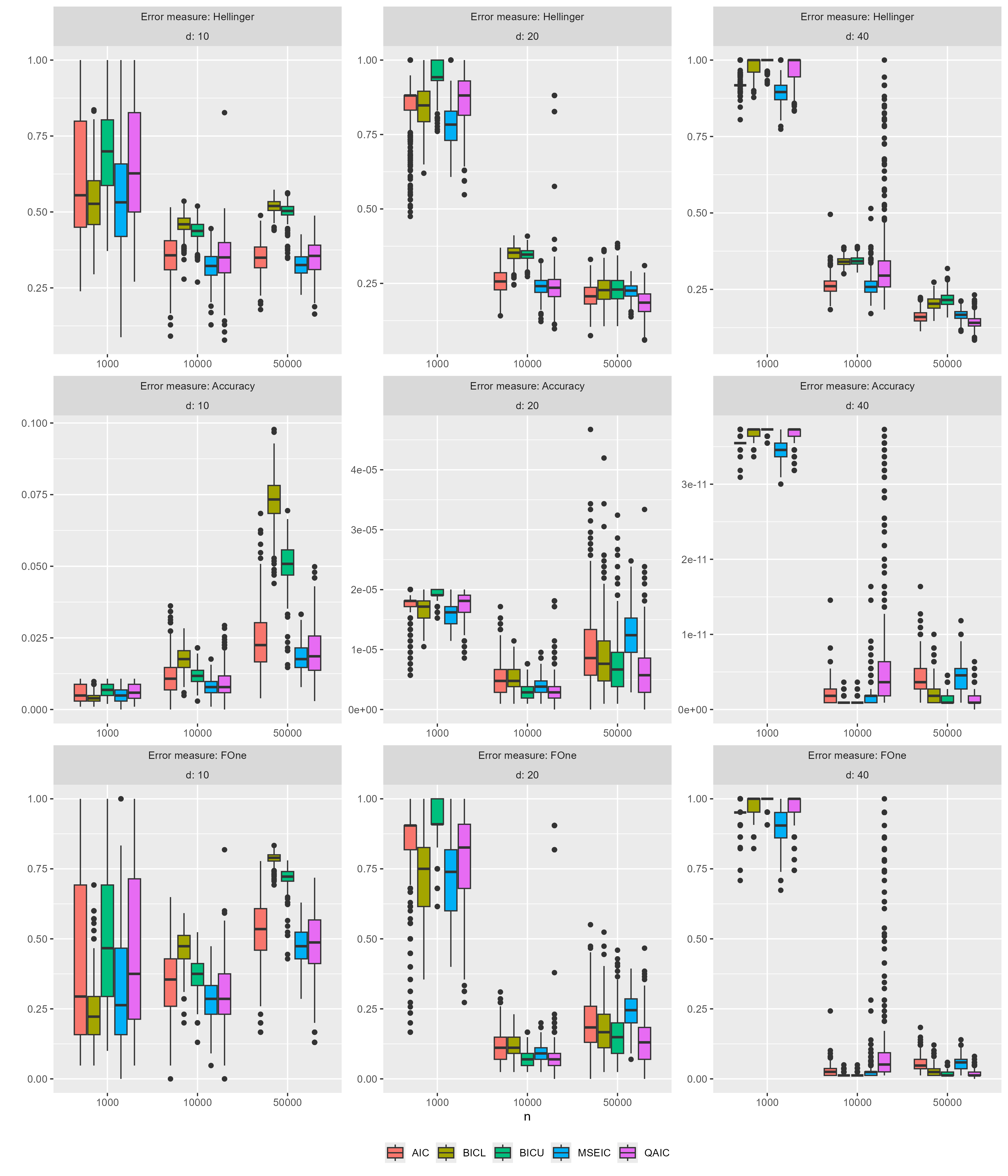
Figure 1: Simulations for asymptotically independent data with $s^{*}=d$ directions of extremes: From left to the right the dimension increases from $d=10$, $d=20$ to $d=40$. In the top row we use as error measure the Hellinger distance, in the middle row the Accuracy Error and in the bottom row the $F_{1}$ Error, which are plotted against the sample size $n$ on the $x$-axis.

The results are presented in Figure 1, where we can see that the error measures behave similarly. For the Hellinger distance, we have an increase in the performance of all information criteria as $n$ grows, except for $d=10$ where the Hellinger distance of the $\operatorname{BICL}$ and $\operatorname{BICU}$ slightly increases from $n=10000$ to $n=50000$. For $d=10$ the Accuracy Error increases if $n$ increases across all information criteria. However, for $d=20$ and $d=40$ the Accuracy and the $F_{1}$ Error appear to be the lowest for data of size $n=10000$ over all information criteria except for $\operatorname{QAIC}$.

7.3 Max-mixture model

Next, we use the max-mixture model of tawn which exhibits asymptotic dependence. Here the spectral measure is not discrete and we need to estimate the support of $\boldsymbol{Z}$ via a Monte-Carlo simulation, where we use the implementation of meyer_muscle23.

For $\beta\in\mathcal{P}_{d}^{*}$ suppose $\boldsymbol{F}_{\beta}=(F_{\beta,j})_{j\in\beta}$ is a $|\beta|$-dimensional random vector with Fréchet(1) distributed margins and the following dependence structure. First, $\boldsymbol{F}_{\{1,2\}},\boldsymbol{F}_{\{4,5\}}$ have a bivariate Gaussian copula with correlation parameter $\rho=0.25$. On the other hand, $\boldsymbol{F}_{\{1,2,3\}},\boldsymbol{F}_{\{3,4,5\}}$ and $\boldsymbol{F}_{\{1,2,3,4,5\}}$ have a three-dimensional and five-dimensional extreme value logistic copula, respectively, with dependence parameter $\vartheta$. Then the regular varying vector $\boldsymbol{X}\in\mathbb{R}^{5}$ of index $-1$ is defined as

$$\boldsymbol{X}\coloneqq(X_{1},\ldots,X_{5})^{\top}\coloneqq\begin{pmatrix}\max\Big{\{}\frac{5}{7}F_{\{1,2\},1},\,\frac{1}{7}F_{\{1,2,3\},1},\,\frac{1}{7}F_{\{1,2,3,4,5\},1}\Big{\}}\\ \max\Big{\{}\frac{5}{7}F_{\{1,2\},2},\,\frac{1}{7}F_{\{1,2,3\},2},\,\frac{1}{7}F_{\{1,2,3,4,5\},2}\Big{\}}\\ \max\Big{\{}\frac{3}{7}F_{\{1,2,3\},3},\,\frac{3}{7}F_{\{3,4,5\},3},\,\frac{1}{7}F_{\{1,2,3,4,5\},3}\Big{\}}\\ \max\Big{\{}\frac{5}{7}F_{\{4,5\},4},\,\frac{1}{7}F_{\{3,4,5\},4},\,\frac{1}{7}F_{\{1,2,3,4,5\},4}\Big{\}}\\ \max\Big{\{}\frac{5}{7}F_{\{4,5\},5},\,\frac{1}{7}F_{\{3,4,5\},5},\,\frac{1}{7}F_{\{1,2,3,4,5\},5}\Big{\}}\\ \end{pmatrix}.$$

Since the Gaussian copula exhibits pairwise asymptotic independence, the random vector $\boldsymbol{Z}$ puts mass on the cones $C_{\{1\}},\,C_{\{2\}},\,C_{\{4\}},\,C_{\{5\}},\,C_{\{1,2,3\}},\,C_{\{3,4,5\}},\,C_{\{1,2,3,4,5\}}$ and by the choice of the scaling factors, each cone has the same probability.

The simulation results of $500$ repetitions and sample sizes $n=1000,10000,50000$ are given in Figure 2.

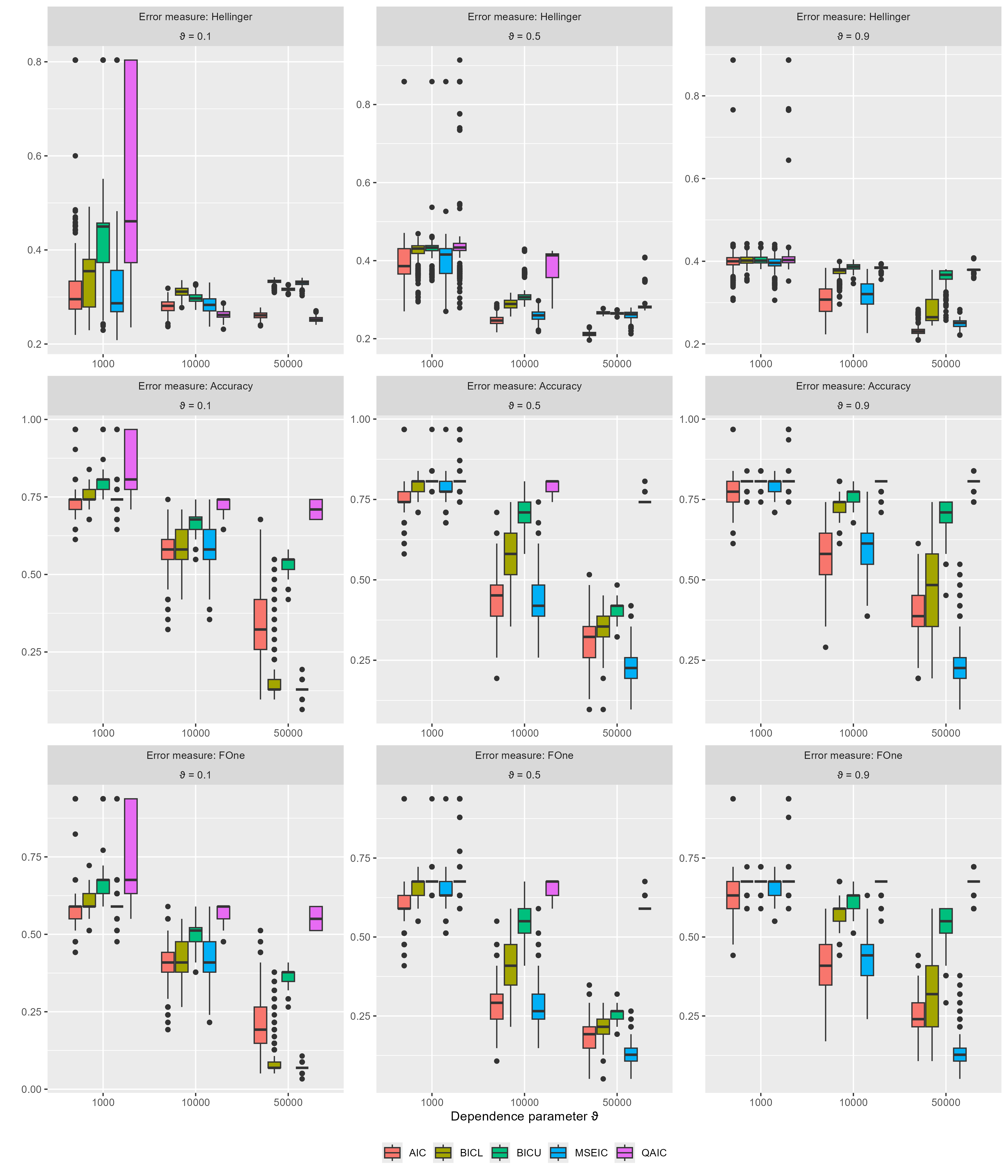
Figure 2: Simulations for max-mixture data: From left to the right the dependence parameter increases from $\vartheta=0.1$, $\vartheta=0.5$ to $\vartheta=0.9$. The number of directions of extremes $s^{*}$ is estimated by a Monte-Carlo simulation. In the top row we use as error measure the Hellinger distance, in the middle row the Accuracy Error and in the bottom row the $F_{1}$ Error, which are plotted against the sample size $n$ on the $x$-axis.

The figure shows similar patterns of all information criteria and in particular, that the overall performance of the information criteria decreases when the dependence parameter $\vartheta$ increases, except for the $\operatorname{QAIC}$ when $n=1000$. Thus, an increase in dependency hurts the quality of the estimation. In this example, a higher sample size $n$ results in an improvement of the accuracy and the $F_{1}$ Error, particularly for $\operatorname{AIC}$ and $\operatorname{MSEIC}$ which have for $\vartheta=0.5$ and $\vartheta=0.9$ the lowest Accuracy Error and $F_{1}$ Error over all information criteria. In general, the behavior of the $F_{1}$ Error is similar to the Accuracy Error in all situations. One noteworthy aspect is that we do not know the true distribution of $\boldsymbol{Z}$, we estimated it via a Monte Carlo simulation. As a result, there occurred a few directions in $\boldsymbol{Z}$ with very small probability mass, which can influence the Error measures.

8 Application to real-world data

In this section, we examine the dependence structure of extreme wind speeds using the same example as meyer_muscle23. For this purpose, the daily average wind speed at $12$ synoptic meteorological stations in the Republic of Ireland from 1961 until 1978 with $n=6574$ observations are considered. The data was subject to HR89 and taken from StatLibData. To what extent dependencies exist, that are not due to the geographical proximity, will be analyzed in the following. The locations of the stations are shown in Figure 4 and consist of: Belmullet (BEL), Birr (BIR), Claremorris (CLA), Clones (CLO), Dublin (DUB), Kilkenny (KIL), Malin Head (MAL), Mullingar (MUL), Roche’s Pt. (RPT), Rosslare (ROS), Shannon (SHA) and Valentia (VAL). For the preprocessing, we use the same Hill estimator $\widehat{\alpha}=10.7$ as meyer_muscle23. We considered values of $k_{n}$ between $33$ and $1183$.

The values of the estimators for $k_{n},k_{n}/n$, and $s^{*}$ are presented in Table 1.

IC	$\widehat{k}$	$\widehat{k}/n$	$\widehat{s}$
$\operatorname{AIC}$	460	0.07	11
$\operatorname{BICU}$	1118	0.17	12
$\operatorname{BICL}$	1118	0.17	13
$\operatorname{MSEIC}$	230	0.03	9
$\operatorname{QAIC}$	592	0.09	11

Table 1: Estimators for the wind speed data set based on the different information criteria.

The number of extreme observations $k_{n}$ varies between $230$ and $1118$, which corresponds to $3\%$ to $17\%$ of the data. However, the information criteria reported between $9$ and $13$ number of extreme directions, which is not a large range compared to the choice of $k_{n}$. On the left-hand side of Figure 3, the values of the information criteria are plotted against the threshold $k_{n}$, while on the right-hand side, the number of estimated directions is mapped as well against $k_{n}$. The vertical lines indicate the minimum of the information criteria. It appears that for the number $s$ of extremal directions, there is a more distinct plateau around the optimal value $\widehat{k}_{n}$ for $\operatorname{BICU},\operatorname{MSEIC}$ and $\operatorname{QAIC}$ compared to $\operatorname{AIC}$ and $\operatorname{BICL}$.

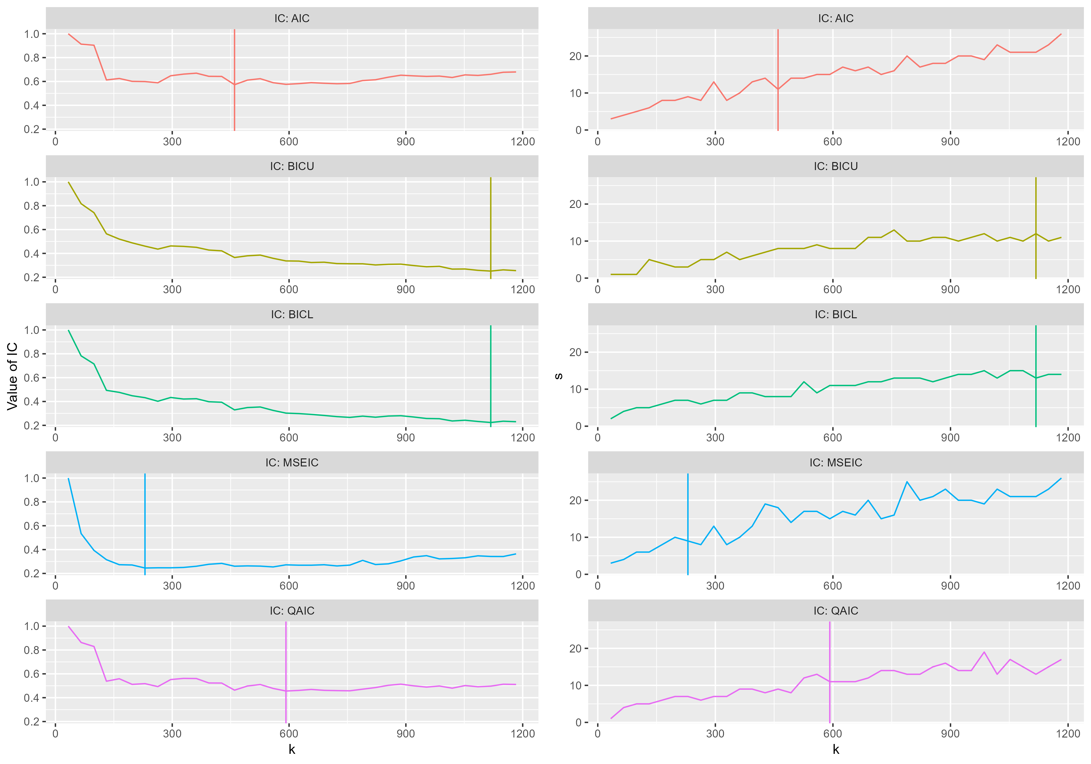
Figure 3: On the left-hand side in the figure the value of the information criteria (IC) and on the right-hand side, the number $s$ of extremal directions is plotted against $k_{n}$. The values of the IC are scaled, such that they start at $1$. The vertical lines indicate the minimum value of the information criteria.

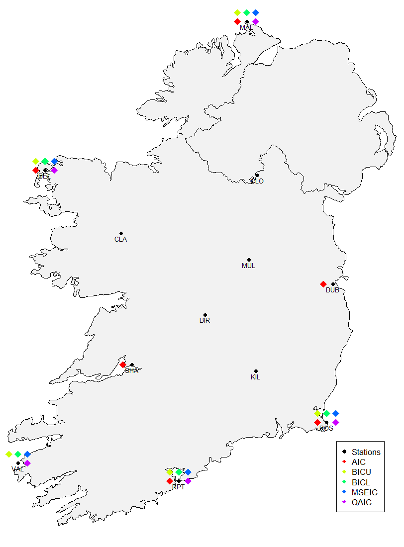
Figure 4: Maximal subsets recovered by the information criteria of the daily average wind speed.

A graphic of the Republic of Ireland is given in Figure 4, where the black dots highlight the different locations of the stations. Colored diamonds close to a station are markers for estimated extreme wind speeds at that station based on an information criterion. All information criteria only identify stations on the coast as extreme, all inland stations have non-extreme wind speeds. $\operatorname{AIC}$ missed one station on the coast, which is Valentia located more than $130$ km away from the other stations. $\operatorname{MSEIC},\operatorname{QAIC},\operatorname{BICU}$ and $\operatorname{BICL}$ recovered the same maximal clusters and missed the coastal stations Shannon and Dublin. The first station, Shannon, is connected to the ocean but nearly $40$ kilometers away from the open sea. The second station, Dublin, is oriented towards the Irish Sea, rather than the Atlantic Ocean. All information criteria identified Belmullet, Mullingar, Rosslare and Roche’s Pt., and four out of five information criteria also recognized Valentia.

9 Conclusion

In this paper, we developed three different information criteria for both the number of extreme directions $s^{*}$ as well as for the choice of the optimal threshold $k_{n}$. Where the BIC is based on a Bayesian approach for a multinomial model in analogy to the $\operatorname{AIC}$ of meyer_muscle23, the $\operatorname{QAIC}$ uses the ideas of an Akaike information criteria but it is based on a Gaussian likelihood function in comparison to the AIC. In contrast, for $\operatorname{MSEIC}$ no likelihood assumption is necessary, it uses the MSE. The advantage of $\operatorname{BICU}$, $\operatorname{BICL}$ and $\operatorname{QAIC}$ is that they are weakly consistent information criteria for the extreme direction $s^{*}$, where AIC and $\operatorname{MSEIC}$ tend to overestimate $s^{*}$ for large sample sizes, although we do not see this phenomenon in the simulations. In particular, $\operatorname{MSEIC}$ performs extraordinarily well in all simulations but all information criteria performed quite well, none is particularly superior in all situations. Finally, the information criteria were successfully applied to a real-world data set, where $\operatorname{MSEIC}$, $\operatorname{QAIC}$, $\operatorname{BICU}$ and $\operatorname{BICL}$ detected the same extreme clusters.

Appendix A Proofs

A.1 Proofs of Section 3

Proof of Theorem 3.1.

Step 1: Suppose $s>{s^{*}}$. By the definition of the $\operatorname{AIC}$ and the log-likelihood function in section 2.4.1 it follows that

$$\operatorname{AIC}_{k_{n}}(s) -\operatorname{AIC}_{k_{n}}(s^{*})$$

$$= -\log L_{M^{s}_{k_{n}}}(\widehat{\boldsymbol{p}}_{n}^{s}\,|\,\boldsymbol{T}_{n}(k_{n}))+s+\log L_{M^{s^{*}}_{k_{n}}}(\widehat{\boldsymbol{p}}_{n}^{s^{*}}\,|\,\boldsymbol{T}_{n}(k_{n}))-{s^{*}}$$

$$= -\sum_{j=s^{*}+1}^{s}T_{n,j}(k_{n})\log\left(\frac{T_{n,j}(k_{n})}{k_{n}}\right)-\log\left(\frac{1}{r-s}\sum_{j=s+1}^{r}\frac{T_{n,j}(k_{n})}{k_{n}}\right)\sum_{i=s+1}^{r}T_{n,i}(k_{n})$$

$$+\log\left(\frac{1}{r-{s^{*}}}\sum_{j={s^{*}}+1}^{r}\frac{T_{n,j}(k_{n})}{k_{n}}\right)\sum_{i={s^{*}}+1}^{r}T_{n,i}(k_{n})+(s-{s^{*}}),$$ (A.1)

where we used that $s>s^{*}$. Inserting the alternative representation

$$T_{n,j}(k_{n})=k_{n}\rho_{n}+\sqrt{k_{n}\rho_{n}}Y_{n,j}$$

where

$$Y_{n,j}\coloneqq\sqrt{k_{n}\rho_{n}}\left(\frac{T_{n,j}(k_{n})}{\rho_{n}k_{n}}-1\right),\quad j=s^{*}+1,\ldots,r,$$

gives that

$$\operatorname{AIC}_{k_{n}}(s) -\operatorname{AIC}_{k_{n}}({s^{*}})$$

$$= -\sum_{j={s^{*}}+1}^{s}(k_{n}\rho_{n}+\sqrt{k_{n}\rho_{n}}Y_{n,j})\log\left(1+\frac{1}{\sqrt{k_{n}\rho_{n}}}Y_{n,j}\right)$$

$$-\log\left(1+\frac{1}{r-s}\sum_{j=s+1}^{r}\frac{1}{\sqrt{k_{n}\rho_{n}}}Y_{n,j}\right)\sum_{i=s+1}^{r}(k_{n}\rho_{n}+\sqrt{k_{n}\rho_{n}}Y_{n,i})$$

$$+\log\left(1+\frac{1}{r-{s^{*}}}\sum_{j={s^{*}}+1}^{r}\frac{1}{\sqrt{k_{n}\rho_{n}}}Y_{n,j}\right)\sum_{i={s^{*}}+1}^{r}(k_{n}\rho_{n}+\sqrt{k_{n}\rho_{n}}Y_{n,i})$$

$$+(s-{s^{*}}).$$ (A.2)

For the asymptotic behavior we apply Assumption (A3) which results in

$$(Y_{n,s^{*}+1},\ldots,Y_{n,r})\overset{\mathcal{D}}{\longrightarrow}(Y_{s^{*}+1},\ldots,Y_{r})\eqqcolon\boldsymbol{Y}\sim\mathcal{N}_{r-s^{*}}(\textbf{0}_{r-s},\boldsymbol{I}_{r-s^{*}}),\quad n\rightarrow\infty,$$ (A.3)

and thus,

$$Y_{n,i}=O_{\mathbb{P}}(1)\quad\text{ for }\quad i=s^{*}+1,\ldots,r.$$

This and the Taylor expansion of the logarithm

$$\log(1+x)=x-\frac{1}{2}x^{2}+O(x^{3}),\quad x\rightarrow 0,$$

we insert in A.2 such that

$$\operatorname{AIC}_{k_{n}}(s) -\operatorname{AIC}_{k_{n}}({s^{*}})$$

$$= -\sum_{j={s^{*}}+1}^{s}(k_{n}\rho_{n}+\sqrt{k_{n}\rho_{n}}Y_{n,j})\left(\frac{1}{\sqrt{k_{n}\rho_{n}}}Y_{n,j}-\frac{1}{2}\frac{1}{k_{n}\rho_{n}}Y_{n,j}^{2}\right)$$

$$-\bigg{(}\frac{1}{r-s}\sum_{j=s+1}^{r}\frac{1}{\sqrt{k_{n}\rho_{n}}}Y_{n,j}-\frac{1}{2}\Big{(}\frac{1}{r-s}\sum_{j=s+1}^{r}\frac{1}{\sqrt{k_{n}\rho_{n}}}Y_{n,j}\Big{)}^{2}\bigg{)}$$

$$\hskip 199.16928pt\cdot\sum_{i=s+1}^{r}(k_{n}\rho_{n}+\sqrt{k_{n}\rho_{n}}Y_{n,i})$$

$$+\bigg{(}\frac{1}{r-{s^{*}}}\sum_{j={s^{*}}+1}^{r}\frac{1}{\sqrt{k_{n}\rho_{n}}}Y_{n,j}-\frac{1}{2}\Big{(}\frac{1}{r-{s^{*}}}\sum_{j={s^{*}}+1}^{r}\frac{1}{\sqrt{k_{n}\rho_{n}}}Y_{n,j}\Big{)}^{2}\bigg{)}$$

$$\hskip 199.16928pt\cdot\sum_{i={s^{*}}+1}^{r}(k_{n}\rho_{n}+\sqrt{k_{n}\rho_{n}}Y_{n,i})$$

$$+(s-{s^{*}})+O_{\mathbb{P}}((k_{n}\rho_{n})^{-1/2}).$$

Since $k_{n}\rho_{n}\rightarrow\infty$ (Lemma 2.7(a)) we receive

$$\operatorname{AIC}_{k_{n}}(s)-\operatorname{AIC}_{k_{n}}({s^{*}})= -\frac{1}{2}\sum_{j={s^{*}}+1}^{s}Y_{n,j}^{2}-\frac{1}{2(r-s)}\left(\sum_{j=s+1}^{r}Y_{n,j}\right)^{2}$$

$$+\frac{1}{2(r-{s^{*}})}\left(\sum_{j={s^{*}}+1}^{r}Y_{n,j}\right)^{2}+(s-{s^{*}})+o_{\mathbb{P}}(1).$$

Due to A.3 and the continuous mapping theorem we finally obtain as $n\rightarrow\infty$,

$$\operatorname{AIC}_{k_{n}}(s)-\operatorname{AIC}_{k_{n}}({s^{*}})\overset{\mathcal{D}}{\longrightarrow} -\frac{1}{2}\sum_{j={s^{*}}+1}^{s}Y_{j}^{2}-\frac{1}{2(r-s)}\bigg{(}\sum_{j=s+1}^{r}Y_{j}\bigg{)}^{\!2}$$

$$+\frac{1}{2(r-{s^{*}})}\bigg{(}\sum_{j={s^{*}}+1}^{r}Y_{j}\bigg{)}^{\!2}+(s-{s^{*}}).$$ (A.4)

Obviously,

$$\mathbb{P} \Biggl{(}-\frac{1}{2}\sum_{j={s^{*}}+1}^{s}Y_{j}^{2}-\frac{\left(\sum_{j=s+1}^{r}Y_{j}\right)^{2}}{2(r-s)}+\frac{\left(\sum_{j={s^{*}}+1}^{r}Y_{j}\right)^{2}}{2(r-{s^{*}})}+s-{s^{*}}<0\Biggr{)}>0.$$

Step 2: Suppose $s<{s^{*}}$. We obtain analog to A.1 that

$$\operatorname{AIC}_{k_{n}}(s) -\operatorname{AIC}_{k_{n}}({s^{*}})$$

$$=\sum_{j=s+1}^{{s^{*}}}T_{n,j}\log\left(\frac{T_{n,j}(k_{n})}{k_{n}}\right)-\log\left(\frac{1}{r-s}\sum_{j=s+1}^{r}\frac{T_{n,j}(k_{n})}{k_{n}}\right)\sum_{i=s+1}^{r}T_{n,i}$$

$$\qquad+\log\left(\frac{1}{r-{s^{*}}}\sum_{j={s^{*}}+1}^{r}\frac{T_{n,j}(k_{n})}{k_{n}}\right)\sum_{i={s^{*}}+1}^{r}T_{n,i}+(s-{s^{*}}).$$ (A.5)

A direct consequence of $T_{n,j}(k_{n})/k_{n}\overset{\mathbb{P}}{\longrightarrow}0$ for $j={s^{*}}+1,\ldots,r$ (Lemma 2.7(c)) and $\lim_{x\rightarrow 0}x\log(x)=0$ is that

$$\log\left(\frac{1}{r-{s^{*}}}\sum_{j={s^{*}}+1}^{r}\frac{T_{n,j}(k_{n})}{k_{n}}\right)\sum_{i={s^{*}}+1}^{r}\frac{T_{n,i}(k_{n})}{k_{n}}\overset{\mathbb{P}}{\longrightarrow}0.$$

Furthermore, Lemma 2.7(b) yields $T_{n,j}(k_{n})/k_{n}\overset{\mathbb{P}}{\longrightarrow}p_{j}>0$ for $j=1,\ldots,{s^{*}}$ and thus, as $n\rightarrow\infty$,

$$\sum_{i=s+1}^{{s^{*}}} \frac{T_{n,i}(k_{n})}{k_{n}}\log\left(\frac{T_{n,i}(k_{n})}{k_{n}}\right)-\log\left(\frac{1}{r-s}\sum_{j=s+1}^{r}\frac{T_{n,j}(k_{n})}{k_{n}}\right)\sum_{i=s+1}^{r}\frac{T_{n,i}(k_{n})}{k_{n}}$$

$$\overset{\mathcal{D}}{\longrightarrow}\sum_{i=s+1}^{{s^{*}}}p_{i}\left(\log\left(p_{i}\right)-\log\left(\frac{1}{r-s}\sum_{j=s+1}^{s^{*}}p_{j}\right)\right),$$ (A.6)

while we used $p_{i}=0$ for $s^{*}\leq i\leq r$. Next, we apply the log sum inequality (Log_Sum_ineq, Theorem 2.7.1) to the limit of A.6 and receive

$$\sum_{i=s+1}^{{s^{*}}} p_{i}\left(\log\left(p_{i}\right)-\log\left(\frac{1}{r-s}\sum_{j=s+1}^{s^{*}}p_{j}\right)\right)=\sum_{i=s+1}^{{s^{*}}}p_{i}\log\left(\frac{p_{i}}{\frac{1}{r-s}\sum_{j=s+1}^{s^{*}}p_{j}}\right)$$

$$\geq\left(\sum_{i=s+1}^{{s^{*}}}p_{i}\right)\log\left(\frac{\sum_{i=s+1}^{{s^{*}}}p_{i}}{\frac{s^{*}-s}{r-s}\sum_{j=s+1}^{s^{*}}p_{j}}\right)=\left(\sum_{i=s+1}^{{s^{*}}}p_{i}\right)\log\left(\frac{r-s}{s^{*}-s}\right)>0,$$ (A.7)

since $r>s^{*}$. Dividing A.5 by $k_{n}$ and using A.6 and A.7 gives

$$\frac{1}{k_{n}}(\operatorname{AIC}_{k_{n}}(s) -\operatorname{AIC}_{k_{n}}({s^{*}}))\overset{\mathcal{D}}{\longrightarrow}\sum_{i=s+1}^{{s^{*}}}p_{i}\left(\log\left(p_{i}\right)-\log\left(\frac{1}{r-s}\sum_{j=s+1}^{s^{*}}p_{j}\right)\right)>0,$$

and thus, the assertion follows. ∎

A.2 Proofs of Section 4

A.2.1 Proof of Theorem 4.2

In the next two lemmata, we derive auxiliary results used for the derivation of an upper bound of the posterior probability $\mathbb{P}(M^{s}_{k_{n}}|\boldsymbol{T}_{n}(k_{n}))$. First, in Lemma A.1, we give a Taylor approximation of the log-likelihood function $\log(L_{M^{s}_{k_{n}}}(\,\cdot\,|\boldsymbol{T}_{n}(k_{n})))$ of Model $M^{s}_{k_{n}}$, and second, in Lemma A.2, we present boundaries for the eigenvalues of the Hessian of the log-likelihood function; the proofs of these auxiliary results are included in Section B.1 of the Supplementary Material. Finally, for the proof of the upper bound of the log-posterior distribution in Theorem 4.2 we combine these two results.

Lemma A.1.

Let the assumptions of Theorem 4.2 hold. Define the ball

$$U_{\varepsilon_{n,\gamma}}(\widehat{\boldsymbol{p}}_{n}^{s})\coloneqq\{\widetilde{\boldsymbol{p}}^{s}\in\Theta_{s}:\|\widetilde{\boldsymbol{p}}^{s}-\widehat{\boldsymbol{p}}_{n}^{s}\|_{2}<\varepsilon_{n,\gamma}\}$$

with radius $\varepsilon_{n,\gamma}\coloneqq{(\rho_{n})^{\gamma}}/{2}$ for $\gamma\geq 4/3$ around $\widehat{\boldsymbol{p}}_{n}^{s}$. Then the following statement holds $\begin{aligned} \sup_{\widetilde{\boldsymbol{p}}^{s}\in U_{\varepsilon_{n,\gamma}}(\widehat{\boldsymbol{p}}_{n}^{s})}\bigg{|}&\log L_{M^{s}_{k_{n}}}(\widetilde{\boldsymbol{p}}^{s}\,|\,\boldsymbol{T}_{n}(k_{n}))-\log L_{M^{s}_{k_{n}}}(\widehat{\boldsymbol{p}}_{n}^{s}\,|\,\boldsymbol{T}_{n}(k_{n}))\\ &-\frac{1}{2}(\widetilde{\boldsymbol{p}}^{s}-\widehat{\boldsymbol{p}}_{n}^{s})^{\top}\nabla^{2}\log L_{M^{s}_{k_{n}}}(\widehat{\boldsymbol{p}}^{s}_{n}\,|\,\boldsymbol{T}_{n}(k_{n}))(\widetilde{\boldsymbol{p}}^{s}-\widehat{\boldsymbol{p}}_{n}^{s})\bigg{|}=o_{\mathbb{P}}(1).\end{aligned}$

Lemma A.2.

Let the assumptions of Theorem 4.2 hold. Define $\lambda_{n,2}\coloneqq{k_{n}}/{T_{n,1}(k_{n})}$ and $\lambda_{n,1}\coloneqq{k_{n}}/{T_{n,s}(k_{n})}+{sk_{n}}/\sum_{j=s+1}^{r}T_{n,j}$. For $\widetilde{\boldsymbol{p}}^{s}\in\Theta_{s}$ we have on the one hand,

$$\lambda_{n,2} (\widetilde{\boldsymbol{p}}^{s}-\widehat{\boldsymbol{p}}_{n}^{s})^{\top}(\widetilde{\boldsymbol{p}}^{s}-\widehat{\boldsymbol{p}}_{n}^{s})\leq(\widetilde{\boldsymbol{p}}^{s}-\widehat{\boldsymbol{p}}_{n}^{s})^{\top}\frac{-1}{k_{n}}\nabla^{2}\log L_{M^{s}_{k_{n}}}(\widehat{\boldsymbol{p}}_{n}^{s}\,|\,\boldsymbol{T}_{n}(k_{n}))(\widetilde{\boldsymbol{p}}^{s}-\widehat{\boldsymbol{p}}_{n}^{s})\quad\mathbb{P}\text{-a.s.}$$

and on the other hand,

$$\lambda_{n,1}(\widetilde{\boldsymbol{p}}^{s}-\widehat{\boldsymbol{p}}_{n}^{s})^{\top}(\widetilde{\boldsymbol{p}}^{s}-\widehat{\boldsymbol{p}}_{n}^{s})\geq(\widetilde{\boldsymbol{p}}^{s}-\widehat{\boldsymbol{p}}_{n}^{s})^{\top}\frac{-1}{k_{n}}\nabla^{2}\log L_{M^{s}_{k_{n}}}(\widehat{\boldsymbol{p}}_{n}^{s}\,|\,\boldsymbol{T}_{n}(k_{n}))(\widetilde{\boldsymbol{p}}^{s}-\widehat{\boldsymbol{p}}_{n}^{s})\quad\mathbb{P}\text{-a.s.}$$

Proof of Theorem 4.2..

In the following let $\gamma=4/3$ and $\varepsilon_{n}\coloneqq\varepsilon_{n,4/3}=(\rho_{n})^{\,4/3}/{2}$. An application of Lemma A.1, Lemma A.2 and Assumption (C1) give

$$-2\log \mathbb{E}_{g_{s}}[L_{M^{s}_{k_{n}}}(\widetilde{\boldsymbol{p}}^{s}\,|\,\boldsymbol{T}_{n}(k_{n}))]$$

$$\leq -2\log\int_{U_{\varepsilon_{n}}(\widehat{\boldsymbol{p}}_{n}^{s})}L_{M^{s}_{k_{n}}}(\widetilde{\boldsymbol{p}}^{s}\,|\,\boldsymbol{T}_{n}(k_{n}))\,\mathrm{d}\widetilde{\boldsymbol{p}}^{s}-2\log b$$

$$\leq -2\log L_{M^{s}_{k_{n}}}(\widehat{\boldsymbol{p}}_{n}^{s}\,|\,\boldsymbol{T}_{n}(k_{n}))$$

$$-2\log\int_{U_{\varepsilon_{n}}(\widehat{\boldsymbol{p}}_{n}^{s})}\!\exp\Big{\{}\frac{-k_{n}}{2}(\widetilde{\boldsymbol{p}}^{s}-\widehat{\boldsymbol{p}}_{n}^{s})^{\top}\frac{-1}{k_{n}}\nabla^{2}\log L_{M^{s}_{k_{n}}}(\widehat{\boldsymbol{p}}_{n}^{s}\,|\,\boldsymbol{T}_{n}(k_{n}))(\widetilde{\boldsymbol{p}}^{s}-\widehat{\boldsymbol{p}}_{n}^{s})\Big{\}}\!\,\mathrm{d}\widetilde{\boldsymbol{p}}^{s}$$

$$-2\log b+o_{\mathbb{P}}(1)$$

$$\leq -2\log L_{M^{s}_{k_{n}}}(\widehat{\boldsymbol{p}}_{n}^{s}\,|\,\boldsymbol{T}_{n}(k_{n}))-s\log(2\pi)+s\log(k_{n}\lambda_{n,1})-2\log b$$

$$-2\log\int_{U_{\varepsilon_{n}}(\widehat{\boldsymbol{p}}_{n}^{s})}\left(\frac{k_{n}\lambda_{n,1}}{2\pi}\right)^{s/2}\exp\left\{\frac{-1}{2}\frac{(\widetilde{\boldsymbol{p}}^{s}-\widehat{\boldsymbol{p}}_{n}^{s})^{\top}(\widetilde{\boldsymbol{p}}^{s}-\widehat{\boldsymbol{p}}_{n}^{s})}{1/(k_{n}\lambda_{n,1})}\right\}\,\mathrm{d}\widetilde{\boldsymbol{p}}^{s}+o_{\mathbb{P}}(1).$$ (A.8)

The integrand is a $s$-dimensional Gaussian density with expectation vector $\widehat{\boldsymbol{p}}_{n}^{s}$ and covariance matrix $(k_{n}\lambda_{n,1})^{-1}\boldsymbol{I}_{s}$. Furthermore, due to the definition of $\lambda_{n,1}$, Assumption (C3) and Lemma 2.7, the asymptotic behavior

$$0\leq k_{n}\lambda_{n,1}\varepsilon_{n}^{2} =\underbrace{\frac{k_{n}(\rho_{n})^{5/3}}{4}}_{\rightarrow\infty}\underbrace{\left(\frac{k_{n}\rho_{n}}{T_{n,s}(k_{n})}+\frac{sk_{n}\rho_{n}}{\sum_{j=s+1}^{r}T_{n,j}}\right)}_{\overset{\text{\lx@cref{creftypecap~refnum}{cor:Theorem1_MW}}}{\rightarrow}\mathds{1}_{\{s\geq s^{*}\}}+\frac{s}{r-\max(s,s^{*})}}\overset{\mathbb{P}}{\longrightarrow}\infty$$ (A.9)

holds in probability. Let $\boldsymbol{N}\sim\mathcal{N}_{s}(\mathbf{0}_{s},\boldsymbol{I}_{s})$. Since $\left\|\boldsymbol{N}\right\|_{2}^{2}\sim\chi^{2}_{s}$ the Markov inequality yields

$$\int_{U_{\varepsilon_{n}}(\widehat{\boldsymbol{p}}_{n}^{s})} \left(\frac{k_{n}\lambda_{n,1}}{2\pi}\right)^{s/2}\exp\left\{\frac{-1}{2}\frac{(\widetilde{\boldsymbol{p}}^{s}-\widehat{\boldsymbol{p}}_{n}^{s})^{\top}(\widetilde{\boldsymbol{p}}^{s}-\widehat{\boldsymbol{p}}_{n}^{s})}{1/(k_{n}\lambda_{n,1})}\right\}\,\mathrm{d}\widetilde{\boldsymbol{p}}^{s}$$

$$=\mathbb{P}\left(\left.\widehat{\boldsymbol{p}}_{n}^{s}+\frac{1}{\sqrt{(k_{n}\lambda_{n,1})}}\boldsymbol{N}\in U_{\varepsilon_{n}}(\widehat{\boldsymbol{p}}_{n}^{s})\right|\boldsymbol{T}_{n}(k_{n})\right)$$

$$=1-\mathbb{P}\left(\left.\left\|\boldsymbol{N}\right\|_{2}^{2}\geq k_{n}\lambda_{n,1}\varepsilon_{n}^{2}\right|\boldsymbol{T}_{n}(k_{n})\right)$$

$$\geq 1-\frac{s}{k_{n}\lambda_{n,1}\varepsilon_{n}^{2}}\to 1,$$

as $n\to\infty$ almost surely, where we used in the last step A.9. Thus,

$$-2\log\int_{U_{\varepsilon_{n}}(\widehat{\boldsymbol{p}}_{n}^{s})}\left(\frac{k_{n}\lambda_{n,1}}{2\pi}\right)^{s/2}\exp\left\{\frac{-1}{2}\frac{(\widetilde{\boldsymbol{p}}^{s}-\widehat{\boldsymbol{p}}_{n}^{s})^{\top}(\widetilde{\boldsymbol{p}}^{s}-\widehat{\boldsymbol{p}}_{n}^{s})}{1/(k_{n}\lambda_{n,1})}\right\}\,\mathrm{d}\widetilde{\boldsymbol{p}}^{s}=o_{\mathbb{P}}(1).$$ (A.10)

Inserting A.10 into A.8 gives then

$$-2\log \mathbb{E}_{g_{s}}[L_{M^{s}_{k_{n}}}(\widetilde{\boldsymbol{p}}^{s}\,|\,\boldsymbol{T}_{n}(k_{n}))]$$

$$\leq-2\log L_{M^{s}_{k_{n}}}(\widehat{\boldsymbol{p}}_{n}^{s}\,|\,\boldsymbol{T}_{n}(k_{n}))-s\log(2\pi)+s\log(k_{n}\lambda_{n,1})-2\log b+o_{\mathbb{P}}(1).$$

Since $T_{n,j}(k_{n})\geq 1$ for $j=1,\ldots,s$, we receive the upper bound

$$\lambda_{n,1}=\left(\frac{k_{n}}{T_{n,s}(k_{n})}+\frac{sk_{n}}{\sum_{j=s+1}^{r}T_{n,j}}\right)\leq k_{n}\left(1+\frac{s}{r-s}\right)=k_{n}\frac{r}{r-s},$$

and finally,

$$-2\log \mathbb{E}_{g_{s}}[L_{M^{s}_{k_{n}}}(\widetilde{\boldsymbol{p}}^{s}\,|\,\boldsymbol{T}_{n}(k_{n}))]$$

$$\leq-2\log L_{M^{s}_{k_{n}}}(\widehat{\boldsymbol{p}}_{n}^{s}\,|\,\boldsymbol{T}_{n}(k_{n}))-s\log(2\pi)+2s\log\left(k_{n}\sqrt{\frac{r}{r-s}}\right)-2\log b+o_{\mathbb{P}}(1),$$

which is the statement. ∎

A.2.2 Proof of Theorem 4.5

Proof of Theorem 4.5.

(a) Note that

$$\operatorname{BICU}_{k_{n}}(s)=2\operatorname{AIC}_{k_{n}}(s)-2s+2s\log\left(k_{n}\right)+s\log\left(\frac{r}{2\pi(r-s)}\right).$$

We consider now the different cases $s>s^{*}$ and $s<s^{*}$ separately.
Step 1: Suppose $s>s^{*}$. We receive with A.4 that

$$\operatorname{BICU}_{k_{n}}(s )-\operatorname{BICU}_{k_{n}}(s^{*})$$

$$= 2\operatorname{AIC}_{k_{n}}(s)-2s+2s\log\left(k_{n}\right)+s\log\left(\frac{r}{2\pi(r-s)}\right)$$

$$-2\operatorname{AIC}_{k_{n}}(s^{*})+2{s^{*}}-2{s^{*}}\log\left(k_{n}\right)-{s^{*}}\log\left(\frac{r}{2\pi(r-{s^{*}})}\right)$$

$$= 2(s-{s^{*}})\log(k_{n})+O_{\mathbb{P}}\left(1\right).$$

Dividing the last equation by $\log(k_{n})$ results in

$$\frac{\operatorname{BICU}_{k_{n}}(s)-\operatorname{BICU}_{k_{n}}(s^{*})}{\log(k_{n})}\overset{\mathbb{P}}{\longrightarrow}2(s-{s^{*}})>0,$$

where we used $\log(k_{n})\rightarrow\infty$.
Step 2: Suppose $s<s^{*}$. Here we have as in the proof of Theorem 3.1 and due to $\log(k_{n})/k_{n}\to 0$ that

$$\frac{\operatorname{BICU}_{k_{n}}(s)-\operatorname{BICU}_{k_{n}}(s^{*})}{k_{n}}$$

$$\quad=2\frac{\operatorname{AIC}_{k_{n}}(s)-\operatorname{AIC}_{k_{n}}(s^{*})}{k_{n}}+\frac{-2s+2s\log\left(k_{n}\right)+s\log\left(\frac{r}{2\pi(r-s)}\right)}{k_{n}}$$

$$\qquad+\frac{2{s^{*}}-2{s^{*}}\log\left(k_{n}\right)-{s^{*}}\log\left(\frac{r}{2\pi(r-{s^{*}})}\right)}{k_{n}}$$

$$\quad\overset{\mathcal{D}}{\longrightarrow}2\sum_{i=s+1}^{{s^{*}}}p_{i}\Bigg{(}\log\left(p_{i}\right)-\log\Bigg{(}\frac{1}{r-s}\sum_{j=s+1}^{s^{*}}p_{j}\Bigg{)}\Bigg{)}>0,$$

and thus, the assertion follows.

(b)   Again, note that

$$\operatorname{BICL}_{k_{n}}(s)=2\operatorname{AIC}_{k_{n}}(s)-2s+s\log\left(k_{n}\right)+s\log\left(\frac{k_{n}}{2\pi T_{n,1}(k_{n})}\right).$$

By a calculation analog to part (a), the $\operatorname{BICL}$ is also consistent since $s\log\left(\frac{k_{n}}{2\pi T_{n,1}(k_{n})}\right)\overset{\mathbb{P}}{\longrightarrow}s\log\left(\frac{1}{2\pi p_{1}}\right)>0$ as $n\to\infty$. ∎

A.2.3 Proof of Theorem 4.7

First, we derive some auxiliary results before we prove Theorem 4.7. Therefore, note that due (2.6) (cf. Equation (1.23) in the Supplementary Material of meyer_muscle23) and $\sum_{j=1}^{2^{d}-1}T_{n,j}^{\prime}=n-T_{n,2^{d}}^{\prime}$, the likelihood function of Model $M^{\prime s}_{n}$ can be written as

$$L_{M^{\prime s}_{n}}(\widetilde{\boldsymbol{p}}^{\prime s}\,|\,\boldsymbol{T}_{n}^{\prime})=L_{M^{s}_{n-T_{n,2^{d}}^{\prime}}}(\widetilde{\boldsymbol{p}}^{s}\,|\,\boldsymbol{T}_{n,\{1,\ldots,r\}}^{\prime})\cdot L_{\operatorname{Bin}_{n}}(1-\widetilde{q}\,|\,T_{n,2^{d}}^{\prime}),$$ (A.11)

for $\widetilde{\boldsymbol{p}}^{\prime s}=(\widetilde{\boldsymbol{p}}^{s},\widetilde{q})\in\Theta_{s}^{\prime}=\Theta_{s}\times(0,1)$, where

$$L_{\operatorname{Bin}_{n}}(1-\widetilde{q}\,|\,T_{n,2^{d}}^{\prime}):=\left(\binom{n}{T_{n,2^{d}}^{\prime}}\right)(1-\widetilde{q})^{T_{n,2^{d}}^{\prime}}\widetilde{q}^{n-T_{n,2^{d}}^{\prime}}$$ (A.12)

is the likelihood function of the binomial model. Next, we define the following expectations with respect to the Lebesgue measure $\lambda$. Let

$$\begin{array}[]{rl}\mathbb{E}_{\lambda}[L_{M^{s}_{n-T_{n,2^{d}}^{\prime}}}(\widetilde{\boldsymbol{p}}^{s}\,|\,\boldsymbol{T}_{n,\{1,\ldots,r\}}^{\prime})]&\coloneqq\int_{\Theta_{s}}L_{M^{s}_{n-T_{n,2^{d}}^{\prime}}}(\widetilde{\boldsymbol{p}}^{s}\,|\,\boldsymbol{T}_{n,\{1,\ldots,r\}}^{\prime})\,\mathrm{d}\widetilde{\boldsymbol{p}}^{s},\\ \mathbb{E}_{\lambda}[L_{\operatorname{Bin}_{n}}(1-\widetilde{q}\,|\,T_{n,2^{d}}^{\prime})]&\coloneqq\int_{(0,1)}L_{\operatorname{Bin}_{n}}(1-\widetilde{q}\,|\,T_{n,2^{d}}^{\prime})\,\mathrm{d}\widetilde{q}.\end{array}$$ (A.15)

Then taking the expectation and logarithm in A.11 results under Assumption (D1) in

$$-2 \log\mathbb{E}_{g_{s}^{\prime}}[L_{M^{\prime s}_{n}}(\widetilde{\boldsymbol{p}}^{\prime s}\,|\,\boldsymbol{T}_{n}^{\prime})]$$

$$\leq-2\log b^{\prime}-2\log\Big{\{}\int_{\Theta_{s}\times(0,1)}\!L_{M^{s}_{n-T_{n,2^{d}}^{\prime}}}\!(\widetilde{\boldsymbol{p}}^{s}\,|\,\boldsymbol{T}_{n,\{1,\ldots,r\}}^{\prime})\cdot L_{\operatorname{Bin}_{n}}(1-\widetilde{q}\,|\,T_{n,2^{d}}^{\prime})\,\mathrm{d}(\widetilde{\boldsymbol{p}}^{s},\widetilde{q})\Big{\}}$$

$$=-2\log b^{\prime}-2\log\Big{\{}\int_{\Theta_{s}}L_{M^{s}_{n-T_{n,2^{d}}^{\prime}}}(\widetilde{\boldsymbol{p}}^{s}\,|\,\boldsymbol{T}_{n,\{1,\ldots,r\}}^{\prime})\,\mathrm{d}\widetilde{\boldsymbol{p}}^{s}\cdot\int_{(0,1)}L_{\operatorname{Bin}_{n}}(1-\widetilde{q}\,|\,T_{n,2^{d}}^{\prime})\,\mathrm{d}\widetilde{q}\Big{\}}$$

$$=-2\log b^{\prime}-2\log\mathbb{E}_{\lambda}[L_{M^{s}_{n-T_{n,2^{d}}^{\prime}}}(\widetilde{\boldsymbol{p}}^{s}\,|\,\boldsymbol{T}_{n,\{1,\ldots,r\}}^{\prime})]-2\log\mathbb{E}_{\lambda}[L_{\operatorname{Bin}_{n}}(1-\widetilde{q}\,|\,T_{n,2^{d}}^{\prime})].$$ (A.16)

In the following two auxiliary lemmata, we determine upper bounds for the expectation of both summands.

Proposition A.3.

Under Assumptions (B1), (B3) and (D4) the asymptotic upper bound as $n\to\infty$,

$$- 2\mathbb{E}\big{[}\log\mathbb{E}_{\lambda}[L_{M^{s}_{n-T_{n,2^{d}}^{\prime}}}(\widetilde{\boldsymbol{p}}^{s}\,|\,\boldsymbol{T}_{n,\{1,\ldots,r\}}^{\prime})]\big{]}$$

$$\leq-2\mathbb{E}\bigl{[}\log\big{(}(n-T_{n,2^{d}}^{\prime})!\big{)}-(n-T_{n,2^{d}}^{\prime})\left(\log(n-T_{n,2^{d}}^{\prime})-1\right)\bigl{]}$$

$$\quad-2\frac{nq_{n}}{k_{n}}\mathbb{E}[\log L_{M^{s}_{k_{n}}}(\widehat{\boldsymbol{p}}_{n}^{s}(\boldsymbol{T}_{n}(k_{n}))\,|\,\boldsymbol{T}_{n}(k_{n}))]+2s\log\Big{(}k_{n}\sqrt{\frac{r}{2\pi(r-s)}}\Big{)}+C\log(nq_{n}),$$

for a constant $C>0$ independent of $s$ and $n$, holds.

Proposition A.4.

Suppose Assumptions (D3) and (B3) hold. The expectation of the binomial likelihood satisfies as $n\to\infty$ the inequality

$$-2\mathbb{E}[\log\mathbb{E}_{\lambda}[L_{\operatorname{Bin}_{n}}(1-\widetilde{q}\,|\,T_{n,2^{d}}^{\prime})]]\leq -2\log(n!)+2\mathbb{E}[\log((n-T_{n,2^{d}}^{\prime})!)]+2\mathbb{E}[\log(T_{n,2^{d}}^{\prime}!)]$$

$$-2nq_{n}\log(k_{n}/n)+2\log(n)+Cnq_{n},$$

for a constant $C>0$ independent of $s$ and $n$.

Proof of Theorem 4.7..

For the ease of notation we define $x\log x$ as zero if $x=0$. Inserting the bounds derived in Proposition A.3 with constant $C_{1}$ and Proposition A.4 with constant $C_{2}$ into A.16 gives for sufficiently large $n$ that

$$-2\mathbb{E}[ \log\mathbb{E}_{g_{s}^{\prime}}[L_{M^{\prime s}_{n}}(\widetilde{\boldsymbol{p}}^{\prime s}\,|\,\boldsymbol{T}_{n}^{\prime})]]+2\log b^{\prime}$$

$$\leq-2\mathbb{E}[\log\mathbb{E}_{\lambda}[L_{M^{s}_{n-T_{n,2^{d}}^{\prime}}}(\widetilde{\boldsymbol{p}}^{s}\,|\,\boldsymbol{T}_{n,\{1,\ldots,r\}}^{\prime})]]-2\mathbb{E}[\log\mathbb{E}_{\lambda}[L_{\operatorname{Bin}_{n}}(1-\widetilde{q}\,|\,T_{n,2^{d}}^{\prime})]]$$

$$\leq-2\mathbb{E}\bigl{[}\log\big{(}(n-T_{n,2^{d}}^{\prime})!\big{)}-(n-T_{n,2^{d}}^{\prime})\left(\log(n-T_{n,2^{d}}^{\prime})-1\right)\bigr{]}$$

$$\quad-2\frac{nq_{n}}{k_{n}}\mathbb{E}[\log L_{M^{s}_{k_{n}}}(\widehat{\boldsymbol{p}}_{n}^{s}\,|\,\boldsymbol{T}_{n}(k_{n}))]+2s\log\Big{(}k_{n}\sqrt{\frac{r}{2\pi(r-s)}}\Big{)}$$

$$\quad-2\log(n!)+2\mathbb{E}[\log((n-T_{n,2^{d}}^{\prime})!)]+2\mathbb{E}[\log(T_{n,2^{d}}^{\prime}!)]$$

$$\quad-2nq_{n}\log(k_{n}/n)+2\log(n)+(C_{1}+C_{2})nq_{n}$$

$$=\Bigl{\{}-2\log(n!)+2\mathbb{E}\bigl{[}(n-T_{n,2^{d}}^{\prime})\left(\log(n-T_{n,2^{d}}^{\prime})-1\right)\bigl{]}+2\mathbb{E}[\log(T_{n,2^{d}}^{\prime}!)]\Bigr{\}}$$

$$\quad+\Big{\{}-2\frac{nq_{n}}{k_{n}}\mathbb{E}[\log L_{M^{s}_{k_{n}}}(\widehat{\boldsymbol{p}}_{n}^{s}\,|\,\boldsymbol{T}_{n}(k_{n}))]+2s\log\Big{(}k_{n}\sqrt{\frac{r}{2\pi(r-s)}}\Big{)}$$

$$\quad\quad-2nq_{n}\log(k_{n}/n)+2\log(n)\Big{\}}+(C_{1}+C_{2})nq_{n}$$

$$\eqqcolon I_{n,1}+I_{n,2}+(C_{1}+C_{2})nq_{n}.$$ (A.17)

Next, we simplify $I_{n,1}$. Therefore, we use the following calculation. Let $B$ be a positive random variable with finite positive variance. For $u>0$ and $x>0$ we the inequality $\log(x/u)\leq x/u-1$ holds, which is equivalent to $x\log(x)\leq x^{2}/u+x\log(u)-x$. Then we have

$$\mathbb{E}[B\log(B)]\leq\frac{\mathbb{E}[B^{2}]}{u}+\mathbb{E}[B]\log(u)-\mathbb{E}[B],$$

and in particular for $u=\mathbb{E}[B^{2}]/\mathbb{E}[B]$ we receive

$$\mathbb{E}[B\log(B)]\leq\mathbb{E}[B]\log(\mathbb{E}[B^{2}]/\mathbb{E}[B]).$$

Since $\mathbb{E}[T_{n,2^{d}}^{\prime}\mathbbm{1}\{T_{n,2^{d}}^{\prime}>0\}]=\mathbb{E}[T_{n,2^{d}}^{\prime}]=n(1-q_{n})$ and $\mathbb{E}[T_{n,2^{d}}^{\prime 2}\mathbbm{1}\{T_{n,2^{d}}^{\prime}>0\}]=\mathbb{E}[T_{n,2^{d}}^{\prime 2}]=nq_{n}(1-q_{n})$ the previous inequality gives

$$\mathbb{E}[T_{n,2^{d}}^{\prime}\log(T_{n,2^{d}}^{\prime}) \mathbbm{1}\{T_{n,2^{d}}^{\prime}>0\}]$$

$$\leq n(1-q_{n})\log\left(\frac{n^{2}(1-q_{n})^{2}+nq_{n}(1-q_{n})}{n(1-q_{n})}\right)$$

$$=n(1-q_{n})\log\left(n(1-q_{n})+q_{n}\right)$$

$$=n(1-q_{n})\log\left(n(1-q_{n})\right)+n(1-q_{n})\log\left(\frac{n(1-q_{n})+q_{n}}{n(1-q_{n})}\right)$$

$$\leq n(1-q_{n})\log\left(n(1-q_{n})\right)+C_{3}$$ (A.18)

for a constant $C_{3}>0$ independent of $s$ and $n$. Furthermore, we use the inequality

$$n\log n-n<\log(n!)<n\log n-n+\log n+1\,$$ (A.19)

to derive a bound for $\mathbb{E}[\log(T_{n,2^{d}}^{\prime}!)]$. Hence, using the upper bound A.19, A.18 and applying Jensen inequality we receive that

$$\mathbb{E}[ \log(T_{n,2^{d}}^{\prime}!)]$$

$$=\mathbb{E}[\log(T_{n,2^{d}}^{\prime}!)\mathbbm{1}\{T_{n,2^{d}}^{\prime}>0\}]$$

$$\leq\mathbb{E}[T_{n,2^{d}}^{\prime}\log(T_{n,2^{d}}^{\prime})\mathbbm{1}\{T_{n,2^{d}}^{\prime}>0\}]-\mathbb{E}[T_{n,2^{d}}^{\prime}\mathbbm{1}\{T_{n,2^{d}}^{\prime}>0\}]+\mathbb{E}[\log(T_{n,2^{d}}^{\prime}\mathbbm{1}\{T_{n,2^{d}}^{\prime}>0\})]$$

$$\leq n(1-q_{n})\log\left(n(1-q_{n})\right)-n(1-q_{n})+\log\left(n(1-q_{n})\right)+C_{4}$$

for a constant $C_{4}>0$ independent of $s$ and $n$. Additionally to the last inequality, we obtain by A.19 and A.18 (for $n-T_{n,2^{d}}^{\prime}$ instead of $T_{n,2^{d}}^{\prime}$ and $q_{n}$ instead of $1-q_{n}$, respectively) that

$$I_{n,1} =-2\log(n!)+2\mathbb{E}\bigl{[}(n-T_{n,2^{d}}^{\prime})\left(\log(n-T_{n,2^{d}}^{\prime})-1\right)\bigl{]}+2\mathbb{E}[\log(T_{n,2^{d}}^{\prime}!)]$$

$$<-2n\log(n)+2n+2nq_{n}\log(nq_{n})-2nq_{n}+2n(1-q_{n})\log(n(1-q_{n}))$$

$$\qquad-2n(1-q_{n})+2\log(n(1-q_{n}))+C_{5}$$

$$=[-2n\log(n)+2nq_{n}\log(n)+2n(1-q_{n})\log(n(1-q_{n}))]$$

$$\qquad+[2nq_{n}\log(q_{n})+2\log(n(1-q_{n}))+C_{5}]$$

$$\leq 2nq_{n}\log(q_{n})+2\log(n)+C_{5}$$ (A.20)

for some constant $C_{5}>0$ independent of $s$ and $n$ holds, where we used that the bracket in the second last equation is negative.

Combining A.17 and A.20 ends up with

$$-2 \mathbb{E}[\log\mathbb{E}_{g_{s}^{\prime}}[L_{M^{\prime s}_{n}}(\widetilde{\boldsymbol{p}}^{\prime s}\,|\,\boldsymbol{T}_{n}^{\prime})]]$$

$$\leq I_{n,1}+I_{n,2}-2\log b^{\prime}+C_{2}nq_{n}$$

$$\leq -2\frac{nq_{n}}{k_{n}}\mathbb{E}[\log L_{M^{s}_{k_{n}}}(\widehat{\boldsymbol{p}}_{n}^{s}\,|\,\boldsymbol{T}_{n}(k_{n}))]+2s\log\left(k_{n}\sqrt{\frac{r}{2\pi(r-s)}}\right)$$

$$\qquad+nq_{n}\Big{(}2\log\left(\frac{nq_{n}}{k_{n}}\right)+\frac{2\log(n)}{nq_{n}}\Big{)}+nq_{n}\;\max_{i=1,\ldots,5}C_{i}\,$$

$$= 2nq_{n}\left[-\frac{\mathbb{E}[\log L_{M^{s}_{k_{n}}}(\widehat{\boldsymbol{p}}_{n}^{s}\,|\,\boldsymbol{T}_{n}(k_{n}))]}{k_{n}}+\frac{s}{nq_{n}}\log\Bigl{(}k_{n}\sqrt{\frac{r}{2\pi(r-s)}}\Bigr{)}+\frac{\log(n)}{nq_{n}}\right]+Cnq_{n},$$

for a constant $C>0$ independent of $s$ and $n$. ∎

A.3 Proofs of Section 5

A.3.1 Proof of Proposition 5.3

Before we are able to present the proof of Proposition 5.3 we require some auxiliary lemmata whose proofs are moved to Appendix C of the Supplementary Material. In the following, we work with the $r$-dimensional multivariate normal distribution $\mathcal{N}_{r}(k_{n}\underline{\boldsymbol{A}}_{s}({\mkern 1.5mu\underline{\mkern-1.5mu\widetilde{\boldsymbol{p}}\mkern-1.5mu}\mkern 1.5mu}^{s}),k_{n}\mathrm{diag}(\underline{\boldsymbol{A}}_{s}({\mkern 1.5mu\underline{\mkern-1.5mu\widetilde{\boldsymbol{p}}\mkern-1.5mu}\mkern 1.5mu}^{s}))),\;{\mkern 1.5mu\underline{\mkern-1.5mu\widetilde{\boldsymbol{p}}\mkern-1.5mu}\mkern 1.5mu}^{s}\in\mathbb{R}_{+}^{s+1},$ which has a negative log-likelihood function

$$-2\log L_{\mathcal{N}_{r}}({\mkern 1.5mu\underline{\mkern-1.5mu\widetilde{\boldsymbol{p}}\mkern-1.5mu}\mkern 1.5mu}^{s}\,|\,\boldsymbol{\mathcal{T}}_{n})= r\log(2\pi)+r\log(k_{n})+\sum_{j=1}^{s}\log(\mkern 1.5mu\underline{\mkern-1.5mu\widetilde{p}\mkern-1.5mu}\mkern 1.5mu^{s}_{j})+(r-s)\log({\mkern 1.5mu\underline{\mkern-1.5mu\widetilde{\rho}\mkern-1.5mu}\mkern 1.5mu^{s}})$$

$$+k_{n}\bigg{(}\sum_{j=1}^{s}\frac{1}{\mkern 1.5mu\underline{\mkern-1.5mu\widetilde{p}\mkern-1.5mu}\mkern 1.5mu^{s}_{j}}\Big{(}\frac{\mathcal{T}_{n,j}}{k_{n}}-\mkern 1.5mu\underline{\mkern-1.5mu\widetilde{p}\mkern-1.5mu}\mkern 1.5mu^{s}_{j}\Big{)}^{2}+\sum_{j=s+1}^{r}\frac{1}{{\mkern 1.5mu\underline{\mkern-1.5mu\widetilde{\rho}\mkern-1.5mu}\mkern 1.5mu^{s}}}\Big{(}\frac{\mathcal{T}_{n,j}}{k_{n}}-{\mkern 1.5mu\underline{\mkern-1.5mu\widetilde{\rho}\mkern-1.5mu}\mkern 1.5mu^{s}}\Big{)}^{2}\bigg{)}.$$

Lemma A.5.

Suppose the assumptions of Proposition 5.3 hold and ${\mkern 1.5mu\underline{\mkern-1.5mu\widehat{\boldsymbol{p}}\mkern-1.5mu}\mkern 1.5mu}^{s}_{n}(\boldsymbol{\mathcal{T}}_{n})$ is defined analog to ${\mkern 1.5mu\underline{\mkern-1.5mu\widehat{\boldsymbol{p}}\mkern-1.5mu}\mkern 1.5mu}^{s}_{n}(\widetilde{\boldsymbol{\mathcal{T}}}_{n})$ in (5.3). Then as $n\rightarrow\infty$,

$$\boldsymbol{Y}_{n}:= \sqrt{k_{n}}\mathrm{diag}(p_{n,1},\ldots,p_{n,s},\frac{\rho_{n}}{(r-s)},\rho_{n},\ldots,\rho_{n})^{-1/2}\begin{pmatrix}\left({\mkern 1.5mu\underline{\mkern-1.5mu\widehat{\boldsymbol{p}}\mkern-1.5mu}\mkern 1.5mu}^{s}_{n}(\widetilde{\boldsymbol{\mathcal{T}}}_{n})-{\mkern 1.5mu\underline{\mkern-1.5mu\widehat{\boldsymbol{p}}\mkern-1.5mu}\mkern 1.5mu}^{s}_{n}(\boldsymbol{\mathcal{T}}_{n})\right)\\ \left(\frac{\mathcal{T}_{n,s+1}}{k_{n}}-\mkern 1.5mu\underline{\mkern-1.5mu\widehat{\rho}\mkern-1.5mu}\mkern 1.5mu^{s}_{n}(\boldsymbol{\mathcal{T}}_{n})\right)\\ \vdots\\ \left(\frac{\mathcal{T}_{n,r}}{k_{n}}-\mkern 1.5mu\underline{\mkern-1.5mu\widehat{\rho}\mkern-1.5mu}\mkern 1.5mu^{s}_{n}(\boldsymbol{\mathcal{T}}_{n})\right)\\ \end{pmatrix}$$

$$\overset{\mathcal{D}}{\longrightarrow} \;\mathcal{N}_{{r+1}}\left(\mathbf{0}_{r+1},\Sigma\right),$$

where

$$\Sigma\coloneqq\begin{pmatrix}2\boldsymbol{I}_{s+1}&\mathbf{0}_{s\times(r-s)}\\ \mathbf{0}_{(r-s)\times(s+1)}&\,\,\boldsymbol{I}_{r-s}-\frac{\mathbf{1}_{r-s}\mathbf{1}_{r-s}^{\top}}{r-s}\end{pmatrix}.$$

Lemma A.6.

Suppose the assumptions of Proposition 5.3 hold and ${\mkern 1.5mu\underline{\mkern-1.5mu\widehat{\boldsymbol{p}}\mkern-1.5mu}\mkern 1.5mu}^{s}_{n}(\boldsymbol{\mathcal{T}}_{n})$ is defined analog to ${\mkern 1.5mu\underline{\mkern-1.5mu\widehat{\boldsymbol{p}}\mkern-1.5mu}\mkern 1.5mu}^{s}_{n}(\widetilde{\boldsymbol{\mathcal{T}}}_{n})$ in (5.3).

1. Then as $n\rightarrow\infty$,

   $$\nabla\log L_{\mathcal{N}_{r}}({\mkern 1.5mu\underline{\mkern-1.5mu\widehat{\boldsymbol{p}}\mkern-1.5mu}\mkern 1.5mu}^{s}_{n}(\boldsymbol{\mathcal{T}}_{n})\,|\,\boldsymbol{\mathcal{T}}_{n})({\mkern 1.5mu\underline{\mkern-1.5mu\widehat{\boldsymbol{p}}\mkern-1.5mu}\mkern 1.5mu}^{s}_{n}(\widetilde{\boldsymbol{\mathcal{T}}}_{n})-{\mkern 1.5mu\underline{\mkern-1.5mu\widehat{\boldsymbol{p}}\mkern-1.5mu}\mkern 1.5mu}^{s}_{n}(\boldsymbol{\mathcal{T}}_{n}))\overset{\mathbb{P}}{\longrightarrow}0.$$

2. Suppose $\bar{\boldsymbol{p}}_{n}\coloneqq(\bar{p}_{n,1},\ldots,\bar{p}_{n,s},\bar{\rho}_{n})^{\top}\in\mathbb{R}_{+}^{s+1}$ satisfies

   $$\|\bar{\boldsymbol{p}}_{n}-{\mkern 1.5mu\underline{\mkern-1.5mu\widehat{\boldsymbol{p}}\mkern-1.5mu}\mkern 1.5mu}^{s}_{n}(\boldsymbol{\mathcal{T}}_{n})\|\leq\|{\mkern 1.5mu\underline{\mkern-1.5mu\widehat{\boldsymbol{p}}\mkern-1.5mu}\mkern 1.5mu}^{s}_{n}(\widetilde{\boldsymbol{\mathcal{T}}}_{n})-{\mkern 1.5mu\underline{\mkern-1.5mu\widehat{\boldsymbol{p}}\mkern-1.5mu}\mkern 1.5mu}^{s}_{n}(\boldsymbol{\mathcal{T}}_{n})\|,\quad n\in\mathbb{N}.$$

   Then as $n\rightarrow\infty$,

   $$({\mkern 1.5mu\underline{\mkern-1.5mu\widehat{\boldsymbol{p}}\mkern-1.5mu}\mkern 1.5mu}^{s}_{n}(\widetilde{\boldsymbol{\mathcal{T}}}_{n})-{\mkern 1.5mu\underline{\mkern-1.5mu\widehat{\boldsymbol{p}}\mkern-1.5mu}\mkern 1.5mu}^{s}_{n}(\boldsymbol{\mathcal{T}}_{n}))^{\top}\Big{(}\nabla^{2}\log L_{\mathcal{N}_{r}}(\bar{\boldsymbol{p}}_{n}\,|\,\boldsymbol{\mathcal{T}}_{n}) +k_{n}\big{(}\mathrm{diag}(p_{n,1},\ldots,p_{n,s},\rho_{n}/(r-s))^{-1}\big{)}\Big{)}$$

   $$\cdot({\mkern 1.5mu\underline{\mkern-1.5mu\widehat{\boldsymbol{p}}\mkern-1.5mu}\mkern 1.5mu}^{s}_{n}(\widetilde{\boldsymbol{\mathcal{T}}}_{n})-{\mkern 1.5mu\underline{\mkern-1.5mu\widehat{\boldsymbol{p}}\mkern-1.5mu}\mkern 1.5mu}^{s}_{n}(\boldsymbol{\mathcal{T}}_{n}))\overset{\mathbb{P}}{\longrightarrow}0.$$

Proof of Proposition 5.3..

Using a Taylor expansion of $\log L_{\mathcal{N}_{r}}({\mkern 1.5mu\underline{\mkern-1.5mu\widehat{\boldsymbol{p}}\mkern-1.5mu}\mkern 1.5mu}^{s}_{n}(\widetilde{\boldsymbol{\mathcal{T}}}_{n})\,|\,\boldsymbol{\mathcal{T}}_{n})$ around ${\mkern 1.5mu\underline{\mkern-1.5mu\widehat{\boldsymbol{p}}\mkern-1.5mu}\mkern 1.5mu}^{s}_{n}(\boldsymbol{\mathcal{T}}_{n})$ yields the existence of a random vector $\bar{\boldsymbol{p}}_{n}\coloneqq(\bar{p}_{n,1},\ldots,\bar{p}_{n,s},\bar{\rho}_{n})^{\top}$ with

$$\|\bar{\boldsymbol{p}}_{n}-{\mkern 1.5mu\underline{\mkern-1.5mu\widehat{\boldsymbol{p}}\mkern-1.5mu}\mkern 1.5mu}^{s}_{n}(\boldsymbol{\mathcal{T}}_{n})\|\leq\|{\mkern 1.5mu\underline{\mkern-1.5mu\widehat{\boldsymbol{p}}\mkern-1.5mu}\mkern 1.5mu}^{s}_{n}(\widetilde{\boldsymbol{\mathcal{T}}}_{n})-{\mkern 1.5mu\underline{\mkern-1.5mu\widehat{\boldsymbol{p}}\mkern-1.5mu}\mkern 1.5mu}^{s}_{n}(\boldsymbol{\mathcal{T}}_{n})\|$$

such that

$$\log L_{\mathcal{N}_{r}} ({\mkern 1.5mu\underline{\mkern-1.5mu\widehat{\boldsymbol{p}}\mkern-1.5mu}\mkern 1.5mu}^{s}_{n}(\widetilde{\boldsymbol{\mathcal{T}}}_{n})\,|\,\boldsymbol{\mathcal{T}}_{n})$$

$$= \log L_{\mathcal{N}_{r}}({\mkern 1.5mu\underline{\mkern-1.5mu\widehat{\boldsymbol{p}}\mkern-1.5mu}\mkern 1.5mu}^{s}_{n}(\boldsymbol{\mathcal{T}}_{n})\,|\,\boldsymbol{\mathcal{T}}_{n})+\nabla\log L_{\mathcal{N}_{r}}({\mkern 1.5mu\underline{\mkern-1.5mu\widehat{\boldsymbol{p}}\mkern-1.5mu}\mkern 1.5mu}_{n}^{s}(\boldsymbol{\mathcal{T}}_{n})\,|\,\boldsymbol{\mathcal{T}}_{n})\big{(}{\mkern 1.5mu\underline{\mkern-1.5mu\widehat{\boldsymbol{p}}\mkern-1.5mu}\mkern 1.5mu}_{n}^{s}(\widetilde{\boldsymbol{\mathcal{T}}}_{n})-{\mkern 1.5mu\underline{\mkern-1.5mu\widehat{\boldsymbol{p}}\mkern-1.5mu}\mkern 1.5mu}_{n}^{s}(\boldsymbol{\mathcal{T}}_{n})\big{)}$$

$$\;+\frac{1}{2}\big{(}{\mkern 1.5mu\underline{\mkern-1.5mu\widehat{\boldsymbol{p}}\mkern-1.5mu}\mkern 1.5mu}^{s}_{n}(\widetilde{\boldsymbol{\mathcal{T}}}_{n})-{\mkern 1.5mu\underline{\mkern-1.5mu\widehat{\boldsymbol{p}}\mkern-1.5mu}\mkern 1.5mu}^{s}_{n}(\boldsymbol{\mathcal{T}}_{n})\big{)}^{\top}\nabla^{2}\log L_{\mathcal{N}_{r}}(\bar{\boldsymbol{p}}_{n}\,|\,\boldsymbol{\mathcal{T}}_{n})\big{(}{\mkern 1.5mu\underline{\mkern-1.5mu\widehat{\boldsymbol{p}}\mkern-1.5mu}\mkern 1.5mu}^{s}_{n}(\widetilde{\boldsymbol{\mathcal{T}}}_{n})-{\mkern 1.5mu\underline{\mkern-1.5mu\widehat{\boldsymbol{p}}\mkern-1.5mu}\mkern 1.5mu}^{s}_{n}(\boldsymbol{\mathcal{T}}_{n})\big{)}.$$

Applying Lemma A.6 (b) gives

$$\log{} L_{\mathcal{N}_{r}}({\mkern 1.5mu\underline{\mkern-1.5mu\widehat{\boldsymbol{p}}\mkern-1.5mu}\mkern 1.5mu}^{s}_{n}(\widetilde{\boldsymbol{\mathcal{T}}}_{n})\,|\,\boldsymbol{\mathcal{T}}_{n})$$

$$= \log L_{\mathcal{N}_{r}}({\mkern 1.5mu\underline{\mkern-1.5mu\widehat{\boldsymbol{p}}\mkern-1.5mu}\mkern 1.5mu}^{s}_{n}(\boldsymbol{\mathcal{T}}_{n})\,|\,\boldsymbol{\mathcal{T}}_{n})$$

$$-\frac{1}{2}\big{(}{\mkern 1.5mu\underline{\mkern-1.5mu\widehat{\boldsymbol{p}}\mkern-1.5mu}\mkern 1.5mu}^{s}_{n}(\widetilde{\boldsymbol{\mathcal{T}}}_{n})-{\mkern 1.5mu\underline{\mkern-1.5mu\widehat{\boldsymbol{p}}\mkern-1.5mu}\mkern 1.5mu}^{s}_{n}(\boldsymbol{\mathcal{T}}_{n})\big{)}^{\top}k_{n}\mathrm{diag}(p_{n,1},\ldots,p_{n,s},\rho_{n}/(r-s))^{-1}\big{(}{\mkern 1.5mu\underline{\mkern-1.5mu\widehat{\boldsymbol{p}}\mkern-1.5mu}\mkern 1.5mu}^{s}_{n}(\widetilde{\boldsymbol{\mathcal{T}}}_{n})-{\mkern 1.5mu\underline{\mkern-1.5mu\widehat{\boldsymbol{p}}\mkern-1.5mu}\mkern 1.5mu}^{s}_{n}(\boldsymbol{\mathcal{T}}_{n})\big{)}$$

$$+o_{\mathbb{P}}(1).$$

Inserting the definition of $\log L_{\mathcal{N}_{r}}({\mkern 1.5mu\underline{\mkern-1.5mu\widehat{\boldsymbol{p}}\mkern-1.5mu}\mkern 1.5mu}^{s}_{n}(\boldsymbol{\mathcal{T}}_{n})\,|\,\boldsymbol{\mathcal{T}}_{n})$ and $\mkern 1.5mu\underline{\mkern-1.5mu\widehat{p}\mkern-1.5mu}\mkern 1.5mu^{s}_{n,j}(\boldsymbol{\mathcal{T}}_{n})=\frac{\mathcal{T}_{n,j}}{k_{n}}$, $j=1,\ldots,s$, yield

$$\log{} L_{\mathcal{N}_{r}}({\mkern 1.5mu\underline{\mkern-1.5mu\widehat{\boldsymbol{p}}\mkern-1.5mu}\mkern 1.5mu}^{s}_{n}(\widetilde{\boldsymbol{\mathcal{T}}}_{n})\,|\,\boldsymbol{\mathcal{T}}_{n})$$

$$=-\frac{1}{2}r\log(2\pi k_{n})-\frac{1}{2}\sum_{j=1}^{s}\log(\mkern 1.5mu\underline{\mkern-1.5mu\widehat{p}\mkern-1.5mu}\mkern 1.5mu^{s}_{n,j}(\boldsymbol{\mathcal{T}}_{n}))-\frac{1}{2}(r-s)\log(\mkern 1.5mu\underline{\mkern-1.5mu\widehat{\rho}\mkern-1.5mu}\mkern 1.5mu^{s}_{n}(\boldsymbol{\mathcal{T}}_{n}))$$

$$\quad-\frac{1}{2}k_{n}\sum_{j=s+1}^{r}\frac{1}{{\mkern 1.5mu\underline{\mkern-1.5mu\widehat{\rho}\mkern-1.5mu}\mkern 1.5mu_{n}^{s}(\boldsymbol{\mathcal{T}}_{n})}}\left(\frac{\mathcal{T}_{n,j}}{k_{n}}-\mkern 1.5mu\underline{\mkern-1.5mu\widehat{\rho}\mkern-1.5mu}\mkern 1.5mu^{s}_{n}(\boldsymbol{\mathcal{T}}_{n})\right)^{2}$$

$$\quad-\frac{1}{2}\big{(}{\mkern 1.5mu\underline{\mkern-1.5mu\widehat{\boldsymbol{p}}\mkern-1.5mu}\mkern 1.5mu}^{s}_{n}(\widetilde{\boldsymbol{\mathcal{T}}}_{n})-{\mkern 1.5mu\underline{\mkern-1.5mu\widehat{\boldsymbol{p}}\mkern-1.5mu}\mkern 1.5mu}^{s}_{n}(\boldsymbol{\mathcal{T}}_{n})\big{)}^{\!\top}\!k_{n}\mathrm{diag}(p_{n,1},\ldots,p_{n,s},\rho_{n}/(r-s))^{-1}\big{(}{\mkern 1.5mu\underline{\mkern-1.5mu\widehat{\boldsymbol{p}}\mkern-1.5mu}\mkern 1.5mu}^{s}_{n}(\widetilde{\boldsymbol{\mathcal{T}}}_{n})-{\mkern 1.5mu\underline{\mkern-1.5mu\widehat{\boldsymbol{p}}\mkern-1.5mu}\mkern 1.5mu}^{s}_{n}(\boldsymbol{\mathcal{T}}_{n})\big{)}$$

$$\quad+o_{\mathbb{P}}(1).$$

Next, we move some terms on the right-hand side and use ${\rho_{n}}/{{\mkern 1.5mu\underline{\mkern-1.5mu\widehat{\rho}\mkern-1.5mu}\mkern 1.5mu_{n}^{s}(\boldsymbol{\mathcal{T}}_{n})}}\overset{\mathbb{P}}{\longrightarrow}1$ (cf. Lemma 2.7 (c) and the assumption $s\geq s^{*}$) and $\boldsymbol{Y}_{n}$ as defined in Lemma A.5 , which result in

$$\log L_{\mathcal{N}_{r}}({\mkern 1.5mu\underline{\mkern-1.5mu\widehat{\boldsymbol{p}}\mkern-1.5mu}\mkern 1.5mu}^{s}_{n}(\widetilde{\boldsymbol{\mathcal{T}}}_{n})\,|\,\boldsymbol{\mathcal{T}}_{n})+\frac{1}{2}r\log(2\pi k_{n})+\frac{1}{2}\sum_{j=1}^{s}\log(\mkern 1.5mu\underline{\mkern-1.5mu\widehat{p}\mkern-1.5mu}\mkern 1.5mu^{s}_{n,j}(\boldsymbol{\mathcal{T}}_{n}))+\frac{1}{2}(r-s)\log(\mkern 1.5mu\underline{\mkern-1.5mu\widehat{\rho}\mkern-1.5mu}\mkern 1.5mu^{s}_{n}(\boldsymbol{\mathcal{T}}_{n}))$$

$$= -\frac{1}{2}k_{n}\sum_{j=s+1}^{r}\frac{1}{{\rho}_{n}}\left(\frac{\mathcal{T}_{n,j}}{k_{n}}-\mkern 1.5mu\underline{\mkern-1.5mu\widehat{\rho}\mkern-1.5mu}\mkern 1.5mu^{s}_{n}(\boldsymbol{\mathcal{T}}_{n})\right)^{2}$$

$$-\frac{1}{2}\big{(}{\mkern 1.5mu\underline{\mkern-1.5mu\widehat{\boldsymbol{p}}\mkern-1.5mu}\mkern 1.5mu}^{s}_{n}(\widetilde{\boldsymbol{\mathcal{T}}}_{n})-{\mkern 1.5mu\underline{\mkern-1.5mu\widehat{\boldsymbol{p}}\mkern-1.5mu}\mkern 1.5mu}^{s}_{n}(\boldsymbol{\mathcal{T}}_{n})\big{)}^{\top}\cdot k_{n}\mathrm{diag}(p_{n,1},\ldots,p_{n,s},\rho_{n}/(r-s))^{-1}\big{(}{\mkern 1.5mu\underline{\mkern-1.5mu\widehat{\boldsymbol{p}}\mkern-1.5mu}\mkern 1.5mu}^{s}_{n}(\widetilde{\boldsymbol{\mathcal{T}}}_{n})-{\mkern 1.5mu\underline{\mkern-1.5mu\widehat{\boldsymbol{p}}\mkern-1.5mu}\mkern 1.5mu}^{s}_{n}(\boldsymbol{\mathcal{T}}_{n})\big{)}$$

$$+o_{\mathbb{P}}(1)$$

$$= -\frac{1}{2}\boldsymbol{Y}_{n}^{\top}\boldsymbol{Y}_{n}+o_{\mathbb{P}}(1)$$

$$\overset{\mathcal{D}}{\longrightarrow} -\frac{1}{2}\boldsymbol{Y}^{\top}\boldsymbol{Y}$$

by Lemma A.5, where $\boldsymbol{Y}\sim\mathcal{N}_{{r+1}}\left(\mathbf{0}_{r+1},\Sigma\right)$. Since

$$\mathbb{E}[-\frac{1}{2}\boldsymbol{Y}^{\top}\boldsymbol{Y}]=-\frac{1}{2}\mathbb{E}[\text{trace}(\boldsymbol{Y}^{\top}\boldsymbol{Y})]=-\frac{1}{2}\text{trace}(\Sigma)=-\frac{r+s+1}{2}$$

the assertion follows.

∎

A.3.2 Proof of Theorem 5.6

Proof of Theorem 5.6.

Step 1: Suppose $s<{s^{*}}$. We have $\widehat{p}^{s}_{n,j}=\widehat{p}^{s^{*}}_{n,j}$ for $j=1,\ldots,s$ and due to Lemma 2.7(b,c) we have as $n\rightarrow\infty$,

$${\widehat{p}^{{s^{*}}}}_{n,j}\overset{\mathbb{P}}{\longrightarrow}p_{j}>0,\quad j=1,\ldots,s^{*},$$

and similarly ${\widehat{\rho}^{s}}_{n}\overset{\mathbb{P}}{\longrightarrow}\frac{1}{r-s}\sum_{j=s+1}^{s^{*}}p_{j}>0$ as well as ${\widehat{\rho}^{{s^{*}}}}_{n}\overset{\mathbb{P}}{\longrightarrow}0$. Thus,

$$-\sum_{j=s+1}^{s^{*}}\log({\widehat{p}^{s^{*}}}_{n,j})+(r-s)\log({\widehat{\rho}^{s}}_{n})\overset{\mathbb{P}}{\longrightarrow}-\sum_{j=s+1}^{s^{*}}\log(p_{j})+(r-s)\log\sqrt{\frac{1}{r-s}\sum_{j=s+1}^{s^{*}}p_{j}^{2}}$$

and $\log({\widehat{\rho}^{{s^{*}}}}_{n})\overset{\mathbb{P}}{\longrightarrow}-\infty.$ Therefore, we have as $n\rightarrow\infty$,

$$\operatorname{QAIC}_{k_{n}} (s)-\operatorname{QAIC}_{k_{n}}(s^{*})$$

$$= -\sum_{j=s+1}^{s^{*}}\log({\widehat{p}^{s^{*}}}_{n,j})+(r-s)\log({\widehat{\rho}^{s}}_{n})-(r-{s^{*}})\log({\widehat{\rho}^{{s^{*}}}}_{n})+(s-{s^{*}})$$

$$\overset{\mathbb{P}}{\longrightarrow} \;\infty.$$

Step 2: Suppose $s>{s^{*}}$. In this case, we have by Lemma 2.7(b,c) that

$$\frac{{\widehat{p}^{s}}_{n,j}}{\rho_{n}}\overset{\mathbb{P}}{\longrightarrow}1,\quad j={s^{*}}+1,\ldots,s,$$

and similarly ${\widehat{\rho}^{s}}_{n}/\rho_{n}\overset{\mathbb{P}}{\longrightarrow}1$ as well as ${\widehat{\rho}^{{s^{*}}}}_{n}/\rho_{n}\overset{\mathbb{P}}{\longrightarrow}1$. Hence, with the continuous mapping theorem we receive $\log(\widehat{p}^{s}_{n,j}/{\rho_{n}})\overset{\mathbb{P}}{\longrightarrow}0$ for $j={s^{*}}+1,\ldots,s$, $\log({\widehat{\rho}^{s^{*}}_{n}}/{\rho_{n}})\overset{\mathbb{P}}{\longrightarrow}0$ and $\log({\widehat{\rho}^{s}}_{n}/{\rho_{n}})\overset{\mathbb{P}}{\longrightarrow}0$ as $n\rightarrow\infty$. Thus, as $n\rightarrow\infty$,

$$\operatorname{QAIC}_{k_{n}}(s) -\operatorname{QAIC}_{k_{n}}(s^{*})$$

$$=\sum_{j={s^{*}}+1}^{s}\log\left(\frac{{\widehat{p}^{s}}_{n,j}}{\rho_{n}}\right)+(r-s)\log\left(\frac{{\widehat{\rho}^{s}}_{n}}{\rho_{n}}\right)-(r-{s^{*}})\log\left(\frac{{\widehat{\rho}^{{s^{*}}}}_{n}}{\rho_{n}}\right)+(s-{s^{*}})$$

$$\overset{\mathbb{P}}{\longrightarrow}s-{s^{*}}>0,$$

which gives the statement. ∎

A.4 Proofs of Section 6

A.4.1 Proof of Theorem 6.1

The proof of Theorem 6.1 is similar to the proof of Proposition 5.3. In the first step, we start to calculate the Jacobian vector of $\ell^{2}\big{(}{\mkern 1.5mu\underline{\mkern-1.5mu\widetilde{\boldsymbol{p}}\mkern-1.5mu}\mkern 1.5mu}^{s}|\boldsymbol{T}_{n}(k_{n})\big{)}$ for ${\mkern 1.5mu\underline{\mkern-1.5mu\widetilde{\boldsymbol{p}}\mkern-1.5mu}\mkern 1.5mu}^{s}=(\mkern 1.5mu\underline{\mkern-1.5mu\widetilde{p}\mkern-1.5mu}\mkern 1.5mu^{s}_{1},\ldots\mkern 1.5mu\underline{\mkern-1.5mu\widetilde{p}\mkern-1.5mu}\mkern 1.5mu^{s}_{s},\mkern 1.5mu\underline{\mkern-1.5mu\widetilde{\rho}\mkern-1.5mu}\mkern 1.5mu^{s})\in\mathbb{R}_{+}^{s+1}$, which is

$$\nabla\ell^{2}\big{(}{\mkern 1.5mu\underline{\mkern-1.5mu\widetilde{\boldsymbol{p}}\mkern-1.5mu}\mkern 1.5mu}^{s}\,|\,\boldsymbol{T}_{n}(k_{n})\big{)}= k_{n}\Bigg{(}\frac{(\mkern 1.5mu\underline{\mkern-1.5mu\widetilde{p}\mkern-1.5mu}\mkern 1.5mu^{s}_{1})^{2}-\frac{T_{n,1}(k_{n})^{2}}{k_{n}^{2}}}{(\mkern 1.5mu\underline{\mkern-1.5mu\widetilde{p}\mkern-1.5mu}\mkern 1.5mu^{s}_{1})^{2}},\ldots,\frac{(\mkern 1.5mu\underline{\mkern-1.5mu\widetilde{p}\mkern-1.5mu}\mkern 1.5mu^{s}_{s})^{2}-\frac{T_{n,s}(k_{n})^{2}}{k_{n}^{2}}}{(\mkern 1.5mu\underline{\mkern-1.5mu\widetilde{p}\mkern-1.5mu}\mkern 1.5mu^{s}_{s})^{2}},\sum_{j=s+1}^{r}\frac{(\mkern 1.5mu\underline{\mkern-1.5mu\widetilde{\rho}\mkern-1.5mu}\mkern 1.5mu^{s})^{2}-\frac{T_{n,j(k_{n})}^{2}}{k_{n}^{2}}}{(\mkern 1.5mu\underline{\mkern-1.5mu\widetilde{\rho}\mkern-1.5mu}\mkern 1.5mu^{s})^{2}}\Bigg{)}$$

and the Hessian matrix is

$$\nabla^{2}\ell^{2}\big{(}{\mkern 1.5mu\underline{\mkern-1.5mu\widetilde{\boldsymbol{p}}\mkern-1.5mu}\mkern 1.5mu}^{s}\,|\,\boldsymbol{T}_{n}(k_{n})\big{)} =2\mathrm{diag}\Bigg{(}\frac{T_{n,1}(k_{n})^{2}}{k_{n}(\mkern 1.5mu\underline{\mkern-1.5mu\widetilde{p}\mkern-1.5mu}\mkern 1.5mu_{1}^{s})^{3}},\ldots,\frac{T_{n,s}(k_{n})^{2}}{k_{n}(\mkern 1.5mu\underline{\mkern-1.5mu\widetilde{p}\mkern-1.5mu}\mkern 1.5mu_{s}^{s})^{3}},\sum_{j=s+1}^{r}\frac{T_{n,j}(k_{n})^{2}}{k_{n}(\mkern 1.5mu\underline{\mkern-1.5mu\widetilde{\rho}\mkern-1.5mu}\mkern 1.5mu^{s})^{3}}\Bigg{)}.$$

Analog to Lemma A.5 and Lemma A.6 we get the following results.

Lemma A.7.

Suppose Assumption A holds, $s\geq s^{*}$ and ${\mkern 1.5mu\underline{\mkern-1.5mu\widehat{\boldsymbol{p}}\mkern-1.5mu}\mkern 1.5mu}^{s}_{n}(\boldsymbol{T}_{n}(k_{n}))$ is defined analogously to ${\mkern 1.5mu\underline{\mkern-1.5mu\widehat{\boldsymbol{p}}\mkern-1.5mu}\mkern 1.5mu}^{s}_{n}(\widetilde{\boldsymbol{T}}_{n}(k_{n}))$ in (5.3). Then as $n\rightarrow\infty$,

$$\mathbf{U}_{n} \coloneqq\sqrt{k_{n}}\mathrm{diag}\bigg{(}p_{n,1},\ldots,p_{n,s},\frac{\rho_{n}}{(r-s)}\bigg{)}^{-1/2}\left({\mkern 1.5mu\underline{\mkern-1.5mu\widehat{\boldsymbol{p}}\mkern-1.5mu}\mkern 1.5mu}^{s}_{n}(\widetilde{\boldsymbol{T}}_{n}(k_{n}))-{\mkern 1.5mu\underline{\mkern-1.5mu\widehat{\boldsymbol{p}}\mkern-1.5mu}\mkern 1.5mu}^{s}_{n}(\boldsymbol{T}_{n}(k_{n}))\right)$$

$$\overset{\mathcal{D}}{\longrightarrow}\mathcal{N}_{{s+1}}\left(\mathbf{0}_{s+1},\begin{pmatrix}2(\boldsymbol{I}_{s}-\sqrt{\boldsymbol{p}_{\{1,\ldots,s\}}}\sqrt{\boldsymbol{p}_{\{1,\ldots,s\}}}^{\top})&\mathbf{0}_{s}\\ \mathbf{0}_{s}^{\top}&2\end{pmatrix}\right).$$

Lemma A.8.

Suppose Assumption A holds, $s\geq s^{*}$ and ${\mkern 1.5mu\underline{\mkern-1.5mu\widehat{\boldsymbol{p}}\mkern-1.5mu}\mkern 1.5mu}^{s}_{n}(\boldsymbol{T}_{n}(k_{n}))$ is defined analogously to ${\mkern 1.5mu\underline{\mkern-1.5mu\widehat{\boldsymbol{p}}\mkern-1.5mu}\mkern 1.5mu}^{s}_{n}(\widetilde{\boldsymbol{T}}_{n}(k_{n}))$ in (5.3).

1. Then as $n\rightarrow\infty$,

   $$\nabla\ell^{2}\big{(}{\mkern 1.5mu\underline{\mkern-1.5mu\widehat{\boldsymbol{p}}\mkern-1.5mu}\mkern 1.5mu}^{s}_{n}(\boldsymbol{T}_{n}(k_{n}))\,|\,\boldsymbol{T}_{n}(k_{n})\big{)}\big{(}{\mkern 1.5mu\underline{\mkern-1.5mu\widehat{\boldsymbol{p}}\mkern-1.5mu}\mkern 1.5mu}^{s}_{n}(\widetilde{\boldsymbol{T}}_{n}(k_{n}))-{\mkern 1.5mu\underline{\mkern-1.5mu\widehat{\boldsymbol{p}}\mkern-1.5mu}\mkern 1.5mu}^{s}_{n}(\boldsymbol{T}_{n}(k_{n}))\big{)}\overset{\mathbb{P}}{\longrightarrow}0.$$

2. Suppose $\bar{\boldsymbol{p}}_{n}\coloneqq(\bar{p}_{n,1},\ldots,\bar{p}_{n,s},\bar{\rho}_{n})^{\top}\in\mathbb{R}_{+}^{s+1}$ satisfies

   $$\|\bar{\boldsymbol{p}}_{n}-{\mkern 1.5mu\underline{\mkern-1.5mu\widehat{\boldsymbol{p}}\mkern-1.5mu}\mkern 1.5mu}^{s}_{n}(\boldsymbol{T}_{n}(k_{n}))\|\leq\|{\mkern 1.5mu\underline{\mkern-1.5mu\widehat{\boldsymbol{p}}\mkern-1.5mu}\mkern 1.5mu}^{s}_{n}(\widetilde{\boldsymbol{T}}_{n}(k_{n}))-{\mkern 1.5mu\underline{\mkern-1.5mu\widehat{\boldsymbol{p}}\mkern-1.5mu}\mkern 1.5mu}^{s}_{n}(\boldsymbol{T}_{n}(k_{n}))\|,\quad n\in\mathbb{N}.$$

   Then as $n\rightarrow\infty$,

   $$\big{(}{\mkern 1.5mu\underline{\mkern-1.5mu\widehat{\boldsymbol{p}}\mkern-1.5mu}\mkern 1.5mu}^{s}_{n}(\widetilde{\boldsymbol{T}}_{n}(k_{n}))- {\mkern 1.5mu\underline{\mkern-1.5mu\widehat{\boldsymbol{p}}\mkern-1.5mu}\mkern 1.5mu}^{s}_{n}(\boldsymbol{T}_{n}(k_{n}))\big{)}^{\top}$$

   $$\cdot\Bigg{(}\nabla^{2}\ell^{2}\big{(}\bar{\boldsymbol{p}}_{n}\,|\,\boldsymbol{T}_{n}(k_{n})\big{)}-2k_{n}\mathrm{diag}\bigg{(}p_{n,1},\ldots,p_{n,s},\frac{\rho_{n}}{{(r-s)}}\bigg{)}^{-1}\Bigg{)}$$

   $$\cdot\big{(}{\mkern 1.5mu\underline{\mkern-1.5mu\widehat{\boldsymbol{p}}\mkern-1.5mu}\mkern 1.5mu}^{s}_{n}(\widetilde{\boldsymbol{T}}_{n}(k_{n}))-{\mkern 1.5mu\underline{\mkern-1.5mu\widehat{\boldsymbol{p}}\mkern-1.5mu}\mkern 1.5mu}^{s}_{n}(\boldsymbol{T}_{n}(k_{n}))\big{)}\overset{\mathbb{P}}{\longrightarrow}0.$$

Proof of Theorem 6.1.

Using a Taylor expansion of $\ell^{2}({\mkern 1.5mu\underline{\mkern-1.5mu\widehat{\boldsymbol{p}}\mkern-1.5mu}\mkern 1.5mu}^{s}_{n}(\widetilde{\boldsymbol{T}}_{n}(k_{n}))\,|\,\boldsymbol{T}_{n}(k_{n}))$ around ${\mkern 1.5mu\underline{\mkern-1.5mu\widehat{\boldsymbol{p}}\mkern-1.5mu}\mkern 1.5mu}^{s}_{n}(\boldsymbol{T}_{n}(k_{n}))$ yields the existence of a random vector $\bar{\boldsymbol{p}}_{n}\coloneqq(\bar{p}_{n,1},\ldots,\bar{p}_{n,s},\bar{\rho}_{n})^{\top}$ with

$$\|\bar{\boldsymbol{p}}_{n}-{\mkern 1.5mu\underline{\mkern-1.5mu\widehat{\boldsymbol{p}}\mkern-1.5mu}\mkern 1.5mu}^{s}_{n}(\boldsymbol{T}_{n}(k_{n}))\|\leq\|{\mkern 1.5mu\underline{\mkern-1.5mu\widehat{\boldsymbol{p}}\mkern-1.5mu}\mkern 1.5mu}^{s}_{n}(\widetilde{\boldsymbol{T}}_{n}(k_{n}))-{\mkern 1.5mu\underline{\mkern-1.5mu\widehat{\boldsymbol{p}}\mkern-1.5mu}\mkern 1.5mu}^{s}_{n}(\boldsymbol{T}_{n}(k_{n}))\|$$

such that

$$\ell^{2}( {\mkern 1.5mu\underline{\mkern-1.5mu\widehat{\boldsymbol{p}}\mkern-1.5mu}\mkern 1.5mu}^{s}_{n}(\widetilde{\boldsymbol{T}}_{n}(k_{n}))\,|\,\boldsymbol{T}_{n}(k_{n}))$$

$$= \ell^{2}({\mkern 1.5mu\underline{\mkern-1.5mu\widehat{\boldsymbol{p}}\mkern-1.5mu}\mkern 1.5mu}^{s}_{n}(\boldsymbol{T}_{n}(k_{n}))\,|\,\boldsymbol{T}_{n}(k_{n}))+\nabla\ell^{2}({\mkern 1.5mu\underline{\mkern-1.5mu\widehat{\boldsymbol{p}}\mkern-1.5mu}\mkern 1.5mu}_{n}^{s}(\boldsymbol{T}_{n}(k_{n}))\,|\,\boldsymbol{T}_{n}(k_{n}))\big{(}{\mkern 1.5mu\underline{\mkern-1.5mu\widehat{\boldsymbol{p}}\mkern-1.5mu}\mkern 1.5mu}_{n}^{s}(\widetilde{\boldsymbol{T}}_{n}(k_{n}))-{\mkern 1.5mu\underline{\mkern-1.5mu\widehat{\boldsymbol{p}}\mkern-1.5mu}\mkern 1.5mu}_{n}^{s}(\boldsymbol{T}_{n}(k_{n}))\big{)}$$

$$+\frac{1}{2}\big{(}{\mkern 1.5mu\underline{\mkern-1.5mu\widehat{\boldsymbol{p}}\mkern-1.5mu}\mkern 1.5mu}^{s}_{n}(\widetilde{\boldsymbol{T}}_{n}(k_{n}))-{\mkern 1.5mu\underline{\mkern-1.5mu\widehat{\boldsymbol{p}}\mkern-1.5mu}\mkern 1.5mu}^{s}_{n}(\boldsymbol{T}_{n}(k_{n}))\big{)}^{\top}\nabla^{2}\ell^{2}\big{(}\bar{\boldsymbol{p}}_{n}\,|\,\boldsymbol{T}_{n}(k_{n})\big{)}\big{(}{\mkern 1.5mu\underline{\mkern-1.5mu\widehat{\boldsymbol{p}}\mkern-1.5mu}\mkern 1.5mu}^{s}_{n}(\widetilde{\boldsymbol{T}}_{n}(k_{n}))-{\mkern 1.5mu\underline{\mkern-1.5mu\widehat{\boldsymbol{p}}\mkern-1.5mu}\mkern 1.5mu}^{s}_{n}(\boldsymbol{T}_{n}(k_{n}))\big{)}.$$

Applying Lemma A.8 gives

$$\ell^{2} ({\mkern 1.5mu\underline{\mkern-1.5mu\widehat{\boldsymbol{p}}\mkern-1.5mu}\mkern 1.5mu}^{s}_{n}(\widetilde{\boldsymbol{T}}_{n}(k_{n}))\,|\,\boldsymbol{T}_{n}(k_{n}))$$

$$=\ell^{2}({\mkern 1.5mu\underline{\mkern-1.5mu\widehat{\boldsymbol{p}}\mkern-1.5mu}\mkern 1.5mu}^{s}_{n}(\boldsymbol{T}_{n}(k_{n}))\,|\,\boldsymbol{T}_{n}(k_{n}))+\big{(}{\mkern 1.5mu\underline{\mkern-1.5mu\widehat{\boldsymbol{p}}\mkern-1.5mu}\mkern 1.5mu}^{s}_{n}(\widetilde{\boldsymbol{T}}_{n}(k_{n}))-{\mkern 1.5mu\underline{\mkern-1.5mu\widehat{\boldsymbol{p}}\mkern-1.5mu}\mkern 1.5mu}^{s}_{n}(\boldsymbol{T}_{n}(k_{n}))\big{)}^{\top}$$

$$\qquad\cdot k_{n}\mathrm{diag}(p_{n,1},\ldots,p_{n,s},\rho_{n}/(r-s))^{-1}\big{(}{\mkern 1.5mu\underline{\mkern-1.5mu\widehat{\boldsymbol{p}}\mkern-1.5mu}\mkern 1.5mu}^{s}_{n}(\widetilde{\boldsymbol{T}}_{n}(k_{n}))-{\mkern 1.5mu\underline{\mkern-1.5mu\widehat{\boldsymbol{p}}\mkern-1.5mu}\mkern 1.5mu}^{s}_{n}(\boldsymbol{T}_{n}(k_{n}))\big{)}+o_{\mathbb{P}}(1)$$

$$=k_{n}\sum_{j=s+1}^{r}\frac{1}{{\mkern 1.5mu\underline{\mkern-1.5mu\widehat{\rho}\mkern-1.5mu}\mkern 1.5mu_{n}^{s}(\boldsymbol{T}_{n}(k_{n}))}}\left(\frac{T_{n,j}(k_{n})}{k_{n}}-\mkern 1.5mu\underline{\mkern-1.5mu\widehat{\rho}\mkern-1.5mu}\mkern 1.5mu^{s}_{n}(\boldsymbol{T}_{n}(k_{n}))\right)^{2}+\big{(}{\mkern 1.5mu\underline{\mkern-1.5mu\widehat{\boldsymbol{p}}\mkern-1.5mu}\mkern 1.5mu}^{s}_{n}(\widetilde{\boldsymbol{T}}_{n}(k_{n}))-{\mkern 1.5mu\underline{\mkern-1.5mu\widehat{\boldsymbol{p}}\mkern-1.5mu}\mkern 1.5mu}^{s}_{n}(\boldsymbol{T}_{n}(k_{n}))\big{)}^{\top}$$

$$\qquad\cdot k_{n}\mathrm{diag}(p_{n,1},\ldots,p_{n,s},\rho_{n}/(r-s))^{-1}\big{(}{\mkern 1.5mu\underline{\mkern-1.5mu\widehat{\boldsymbol{p}}\mkern-1.5mu}\mkern 1.5mu}^{s}_{n}(\widetilde{\boldsymbol{T}}_{n}(k_{n}))-{\mkern 1.5mu\underline{\mkern-1.5mu\widehat{\boldsymbol{p}}\mkern-1.5mu}\mkern 1.5mu}^{s}_{n}(\boldsymbol{T}_{n}(k_{n}))\big{)}+o_{\mathbb{P}}(1).$$

Next, we move some terms on the right-hand side and use Lemma A.7, which result in

$$\ell^{2} ({\mkern 1.5mu\underline{\mkern-1.5mu\widehat{\boldsymbol{p}}\mkern-1.5mu}\mkern 1.5mu}^{s}_{n}(\widetilde{\boldsymbol{T}}_{n}(k_{n}))\,|\,\boldsymbol{T}_{n}(k_{n}))-k_{n}\sum_{j=s+1}^{r}\frac{1}{{\rho}_{n}}\left(\frac{T_{n,j}(k_{n})}{k_{n}}-\mkern 1.5mu\underline{\mkern-1.5mu\widehat{\rho}\mkern-1.5mu}\mkern 1.5mu^{s}_{n}(\boldsymbol{T}_{n}(k_{n}))\right)^{2}$$

$$=\big{(}{\mkern 1.5mu\underline{\mkern-1.5mu\widehat{\boldsymbol{p}}\mkern-1.5mu}\mkern 1.5mu}^{s}_{n}(\widetilde{\boldsymbol{T}}_{n}(k_{n}))-{\mkern 1.5mu\underline{\mkern-1.5mu\widehat{\boldsymbol{p}}\mkern-1.5mu}\mkern 1.5mu}^{s}_{n}(\boldsymbol{T}_{n}(k_{n}))\big{)}^{\top}k_{n}\mathrm{diag}(p_{n,1},\ldots,p_{n,s},\rho_{n}/(r-s))^{-1}$$

$$\quad\qquad\cdot\big{(}{\mkern 1.5mu\underline{\mkern-1.5mu\widehat{\boldsymbol{p}}\mkern-1.5mu}\mkern 1.5mu}^{s}_{n}(\widetilde{\boldsymbol{T}}_{n}(k_{n}))-{\mkern 1.5mu\underline{\mkern-1.5mu\widehat{\boldsymbol{p}}\mkern-1.5mu}\mkern 1.5mu}^{s}_{n}(\boldsymbol{T}_{n}(k_{n}))\big{)}+o_{\mathbb{P}}(1)$$

$$=\mathbf{U}_{n}^{\top}\mathbf{U}_{n}+o_{\mathbb{P}}(1)$$

$$\overset{\mathcal{D}}{\longrightarrow}\mathbf{U}^{\top}\mathbf{U},$$

as $n\to\infty$, where $\mathbf{U}^{\top}\mathbf{U}\sim 2\chi^{2}_{s}$. Since $\mathbb{E}[\mathbf{U}^{\top}\mathbf{U}]=2s$ the assertion follows. ∎

A.4.2 Proof of Theorem 6.3

Proof of Theorem 6.3.

Step 1: Suppose $s<{s^{*}}$. An application of Lemma 2.7(b,c) gives on the one hand,

$$\frac{1}{\sum_{l=s+1}^{r}\frac{T_{n,l}(k_{n})}{k_{n}(r-s)}} \sum_{j=s+1}^{r}\left(\frac{T_{n,j}(k_{n})}{k_{n}}-\sum_{i=s+1}^{r}\frac{T_{n,i}(k_{n})}{k_{n}(r-s)}\right)^{2}$$

$$\overset{\mathbb{P}}{\longrightarrow}\frac{1}{\sum_{l=s+1}^{s^{*}}\frac{p_{l}}{r-s}}\sum_{j=s+1}^{s^{*}}\left(p_{j}-\sum_{i=s+1}^{s^{*}}\frac{p_{i}}{r-s}\right)^{2},$$

where we already applied that $p_{j}=0$ for $j=s^{*},\ldots,r$. Moreover,

$$p_{s+1}-\sum_{i=s+1}^{s^{*}}\frac{p_{i}}{r-s}\geq p_{s+1}-\frac{{s^{*}}-{s}}{r-s}p_{s+1}=\frac{r-{s^{*}}}{r-s}p_{s+1}>0.$$

Hence,

$$\frac{k_{n}}{\sum_{l=s+1}^{r}\frac{T_{n,l}(k_{n})}{k_{n}(r-s)}}\sum_{j=s+1}^{r}\left(\frac{T_{n,j}(k_{n})}{k_{n}}-\sum_{i=s+1}^{r}\frac{T_{n,i}(k_{n})}{k_{n}(r-s)}\right)^{2}\overset{\mathbb{P}}{\longrightarrow}\infty.$$ (A.21)

On the other hand, define

$$\boldsymbol{V}_{n}\coloneqq\sqrt{k_{n}\rho_{n}}\left(\frac{\boldsymbol{T}_{n,{\{{s^{*}}+1,\ldots,r\}}}(k_{n})}{\rho_{n}k_{n}}-\mathbf{1}_{r-s^{*}}\right)\quad\text{ and }\quad\boldsymbol{V}\sim\mathcal{N}_{r-{s^{*}}}(\mathbf{0}_{r-{s^{*}}},\boldsymbol{I}_{r-{s^{*}}}).$$

By Assumption (A3) we have $\boldsymbol{V}_{n}\overset{\mathcal{D}}{\longrightarrow}\boldsymbol{V}.$ Furthermore, since $T_{n,l}(k_{n})/(k_{n}\rho_{n})\overset{\mathbb{P}}{\longrightarrow}1$ for $l={s^{*}}+1,\ldots,r$ by Lemma 2.7(c), it follows that

$$\frac{\rho_{n}}{\sum_{l={s^{*}}+1}^{r}\frac{T_{n,l}(k_{n})}{k_{n}(r-{s^{*}})}}\frac{k_{n}}{\rho_{n}}\sum_{j={s^{*}}+1}^{r}\left(\frac{T_{n,j}(k_{n})}{k_{n}}-\sum_{i={s^{*}}+1}^{r}\frac{T_{n,i}(k_{n})}{k_{n}(r-{s^{*}})}\right)^{2}$$

$$=\underbrace{\frac{\rho_{n}}{\sum_{l={s^{*}}+1}^{r}\frac{T_{n,l}(k_{n})}{k_{n}(r-{s^{*}})}}}_{\overset{\mathbb{P}}{\longrightarrow}1}\underbrace{\boldsymbol{V}_{n}^{\top}(\boldsymbol{I}_{r-{s^{*}}}-\frac{1}{r-{s^{*}}}\mathbf{1}_{r-s^{*}}\mathbf{1}_{r-s^{*}}^{\top})^{\top}(\boldsymbol{I}_{r-{s^{*}}}-\frac{1}{r-{s^{*}}}\mathbf{1}_{r-s^{*}}\mathbf{1}_{r-s^{*}}^{\top})\boldsymbol{V}_{n}}_{\overset{\mathcal{D}}{\longrightarrow}\chi_{r-s^{*}-1}^{2}}$$

$$\overset{\mathcal{D}}{\longrightarrow}\chi_{r-s^{*}-1}^{2}=O_{\mathbb{P}}(1).$$ (A.22)

Combining A.21 and A.22 yields

$$\operatorname{MSEIC}_{k_{n}}(s)- \operatorname{MSEIC}_{k_{n}}(s^{*})$$

$$=2(s-s^{*})+\frac{k_{n}}{\sum_{l=s+1}^{r}\frac{T_{n,l}(k_{n})}{k_{n}(r-s)}}\sum_{j=s+1}^{r}\left(\frac{T_{n,j}(k_{n})}{k_{n}}-\sum_{i=s+1}^{r}\frac{T_{n,i}(k_{n})}{k_{n}(r-s)}\right)^{2}$$

$$\quad-\frac{k_{n}}{\sum_{l={s^{*}}+1}^{r}\frac{T_{n,l}(k_{n})}{k_{n}(r-{s^{*}})}}\sum_{j={s^{*}}+1}^{r}\left(\frac{T_{n,j}(k_{n})}{k_{n}}-\sum_{i={s^{*}}+1}^{r}\frac{T_{n,i}(k_{n})}{k_{n}(r-{s^{*}})}\right)^{2}$$

$$\overset{\mathbb{P}}{\longrightarrow}\infty.$$

Step 2: Suppose $s>{s^{*}}$. An application of (A.22) and Lemma 2.7(c) yield

$$\frac{k_{n}}{\sum_{l={s^{*}}+1}^{r}\frac{T_{n,l}(k_{n})}{k_{n}(r-{s^{*}})}} \sum_{j={s^{*}}+1}^{r}\left(\frac{T_{n,j}(k_{n})}{k_{n}}-\sum_{i={s^{*}}+1}^{r}\frac{T_{n,i}(k_{n})}{k_{n}(r-{s^{*}})}\right)^{2}$$

$$-\frac{k_{n}}{\rho_{n}}\sum_{j={s^{*}}+1}^{r}\left(\frac{T_{n,j}(k_{n})}{k_{n}}-\sum_{i={s^{*}}+1}^{r}\frac{T_{n,i}(k_{n})}{k_{n}(r-{s^{*}})}\right)^{2}$$

$$= \underbrace{\left(\frac{\rho_{n}}{\sum_{l={s^{*}}+1}^{r}\frac{T_{n,l}(k_{n})}{k_{n}(r-{s^{*}})}}-1\right)}_{\overset{\mathbb{P}}{\longrightarrow}0}\underbrace{\frac{k_{n}}{\rho_{n}}\sum_{j={s^{*}}+1}^{r}\left(\frac{T_{n,j}(k_{n})}{k_{n}}-\sum_{i={s^{*}}+1}^{r}\frac{T_{n,i}(k_{n})}{k_{n}(r-{s^{*}})}\right)^{2}}_{\overset{\mathcal{D}}{\longrightarrow}\chi_{r-s^{*}-1}^{2}\text{ by }\eqref{eq:MSE_cons_Term2}}$$

$$={} o_{\mathbb{P}}(1).$$ (A.23)

Since $s>{s^{*}}$ the analog holds when ${s^{*}}$ is replaced by $s$. Using $\boldsymbol{V}_{n}=(V_{n,{s^{*}}+1},\ldots,V_{n,r})^{\top}$ defined as above, we have the representation $\frac{T_{n,j}(k_{n})}{k_{n}\rho_{n}}=\frac{1}{\sqrt{k_{n}\rho_{n}}}V_{n,j}+1.$ Thus, when inserting the definition of $\operatorname{MSEIC}$ we get with A.23 that

$$\operatorname{MSEIC}_{k_{n}}(s)-\operatorname{MSEIC}_{k_{n}}(s^{*})$$

$$={} 2(s-s^{*})+\frac{k_{n}}{\rho_{n}}\sum_{j=s+1}^{r}\left(\frac{T_{n,j}(k_{n})}{k_{n}}-\sum_{i=s+1}^{r}\frac{T_{n,i}(k_{n})}{k_{n}(r-s)}\right)^{2}$$

$$-\frac{k_{n}}{\rho_{n}}\sum_{j={s^{*}}+1}^{r}\left(\frac{T_{n,j}(k_{n})}{k_{n}}-\sum_{i={s^{*}}+1}^{r}\frac{T_{n,i}(k_{n})}{k_{n}(r-{s^{*}})}\right)^{2}+o_{\mathbb{P}}(1)$$

$$={} 2(s-s^{*})+\sum_{j=s+1}^{r}\left\{\sqrt{k_{n}\rho_{n}}\left(\frac{T_{n,j}(k_{n})}{k_{n}\rho_{n}}-1\right)-\frac{\sqrt{k_{n}\rho_{n}}}{(r-s)}\sum_{i=s+1}^{r}\left(\frac{T_{n,i}(k_{n})}{k_{n}\rho_{n}}-1\right)\right\}^{2}$$

$$-\sum_{j={s^{*}}+1}^{r}\left\{\sqrt{k_{n}\rho_{n}}\left(\frac{T_{n,j}(k_{n})}{k_{n}\rho_{n}}-1\right)-\frac{\sqrt{k_{n}\rho_{n}}}{(r-{s^{*}})}\sum_{i={s^{*}}+1}^{r}\left(\frac{T_{n,i}(k_{n})}{k_{n}\rho_{n}}-1\right)\right\}^{2}+o_{\mathbb{P}}(1)$$

$$={} 2(s-s^{*})+\sum_{j=s+1}^{r}\left\{V_{n,j}-\frac{1}{(r-s)}\sum_{i=s+1}^{r}V_{n,i}\right\}^{2}$$

$$-\sum_{j={s^{*}}+1}^{r}\left\{V_{n,j}-\frac{1}{(r-{s^{*}})}\sum_{i={s^{*}}+1}^{r}V_{n,i}\right\}^{2}+o_{\mathbb{P}}(1)$$

$$\overset{\mathcal{D}}{\longrightarrow}{} 2(s-s^{*})+\sum_{j=s+1}^{r}\left\{V_{j}-\frac{1}{(r-s)}\sum_{i=s+1}^{r}V_{i}\right\}^{2}-\sum_{j={s^{*}}+1}^{r}\left\{V_{j}-\frac{1}{(r-{s^{*}})}\sum_{i={s^{*}}+1}^{r}V_{i}\right\}^{2}.$$

Similar to the proof of Theorem 3.1, there exists a positive probability that the right-hand side is positive. Hence, the assertion follows. ∎

A.4.3 Proof of Theorem 6.4

Before we are able to present the proof of Theorem 6.4 we require some auxiliary lemmata whose proofs are moved to Appendix D in the Supplementary Material.

Lemma A.9.

Suppose assumptions (B1) and (B2) hold. Then for $\boldsymbol{p}^{\prime}\in\mathbb{R}_{+}^{r}$ the asymptotic behavior

$$\mathbb{E} \left[\left\|\sqrt{n-T_{n,2^{d}}^{\prime}}\mathrm{diag}(\boldsymbol{p}^{\prime})^{-1/2}\left(\frac{\boldsymbol{T}_{n,\{1,\ldots,r\}}^{\prime}}{n-T_{n,2^{d}}^{\prime}}-\boldsymbol{p}^{\prime}\right)\right\|^{2}_{2}\right]$$

$$\qquad=nq_{n}\left(\frac{1}{k_{n}}\mathbb{E}[\ell^{2}\big{(}\boldsymbol{p}^{\prime}|\boldsymbol{T}_{n}(k_{n})\big{)}]+o\left(\frac{1}{nq_{n}}\right)\right)$$

as $n\to\infty$ holds.

Lemma A.10.

For $q^{\prime}\in(0,1)$ the equality

$$\mathbb{E} \left[\left\|\sqrt{n}(q^{\prime}(1-q^{\prime}))^{-1/2}\left(\frac{T_{n,2^{d}}^{\prime}}{n}-(1-q^{\prime})\right)\right\|^{2}_{2}\right]=nq_{n}\left(\frac{(1-q_{n})}{nq^{\prime}(1-q^{\prime})}+\frac{(q^{\prime}-q_{n})^{2}}{q_{n}q^{\prime}(1-q^{\prime})}\right)$$

holds.

Proof of Theorem 6.4.

For $q^{\prime}\in(0,1)$ and $\boldsymbol{p}^{\prime}\in\mathbb{R}^{r}_{+}$ we have as a consequence of Lemmas A.9 and A.10 that

$$q^{\prime}\mathbb{E} \left[\left\|\sqrt{n-T_{n,2^{d}}^{\prime}}\mathrm{diag}(\boldsymbol{p}^{\prime})^{-1/2}\left(\frac{\boldsymbol{T}_{n,\{1,\ldots,r\}}^{\prime}}{n-T_{n,2^{d}}^{\prime}}-\boldsymbol{p}^{\prime}\right)\right\|^{2}_{2}\right]$$

$$+(1-q^{\prime})\mathbb{E}\left[\left\|\sqrt{n}(q^{\prime}(1-q^{\prime}))^{-1/2}\left(\frac{T_{n,2^{d}}^{\prime}}{n}-(1-q^{\prime})\right)\right\|^{2}_{2}\right]$$

$$=nq_{n}\left(\frac{q^{\prime}}{k_{n}}\mathbb{E}[\ell^{2}\big{(}\boldsymbol{p}^{\prime}|\boldsymbol{T}_{n}(k_{n})\big{)}]+o\left(\frac{q^{\prime}}{nq_{n}}\right)\right)+nq_{n}\left(\frac{(1-q_{n})}{nq^{\prime}}+\frac{(q^{\prime}-q_{n})^{2}}{q_{n}q^{\prime}}\right).$$

Therefore, it follows that

$$\mathbb{E}\Bigg{[}q^{\prime}\mathbb{E} \left[\left\|\sqrt{n-T_{n,2^{d}}^{\prime}}\mathrm{diag}(\boldsymbol{p}^{\prime})^{-1/2}\left(\frac{\boldsymbol{T}_{n,\{1,\ldots,r\}}^{\prime}}{n-T_{n,2^{d}}^{\prime}}-\boldsymbol{p}^{\prime}\right)\right\|^{2}_{2}\right]\bigg{|}_{\boldsymbol{p}^{\prime}=\widehat{\boldsymbol{p}}_{n}(\frac{\widetilde{\boldsymbol{T}}_{n}(k_{n})}{k_{n}}),q^{\prime}=\frac{k_{n}}{n}}\Bigg{]}$$

$$\quad+\mathbb{E}\Bigg{[}(1-q^{\prime})\mathbb{E}\left[\left\|\sqrt{n}(q^{\prime}(1-q^{\prime}))^{-1/2}\left(\frac{T_{n,2^{d}}^{\prime}}{n}-(1-q^{\prime})\right)\right\|^{2}_{2}\right]\bigg{|}_{q^{\prime}=\frac{k_{n}}{n}}\Bigg{]}$$

$$=nq_{n}\mathbb{E}\Bigg{[}\left(\frac{q^{\prime}}{k_{n}}\mathbb{E}[\ell^{2}\big{(}\boldsymbol{p}^{\prime}|\boldsymbol{T}_{n}(k_{n})\big{)}]+o\left(\frac{q^{\prime}}{nq_{n}}\right)\right)\Big{|}_{\boldsymbol{p}^{\prime}=\widehat{\boldsymbol{p}}_{n}(\frac{\widetilde{\boldsymbol{T}}_{n}(k_{n})}{k_{n}}),q^{\prime}=\frac{k_{n}}{n}}\Bigg{]}$$

$$\quad+nq_{n}\mathbb{E}\Bigg{[}\left(\frac{(1-q_{n})}{nq^{\prime}}+\frac{(q^{\prime}-q_{n})^{2}}{q_{n}q^{\prime}}\right)\Big{|}_{q^{\prime}=\frac{k_{n}}{n}}\Bigg{]}$$

$$=nq_{n}\left(\frac{1}{n}\operatorname{MSE}_{k_{n}}(s)+\frac{(1-q_{n})}{k_{n}}+\frac{(\frac{k_{n}}{n}-q_{n})^{2}}{q_{n}\frac{k_{n}}{n}}+o\left(n^{-1}\right)\right).$$

Due to the asymptotic behavior as $n\to\infty$,

$$\frac{(\frac{k_{n}}{n}-q_{n})^{2}}{q_{n}\frac{k_{n}}{n}}+o\left(n^{-1}\right)=\frac{k_{n}(1-\frac{nq_{n}}{k_{n}})^{2}}{nq_{n}}{+o\left(n^{-1}\right)}=o((nq_{n})^{-1})+o\left(n^{-1}\right)=o((nq_{n})^{-1}),$$

where we used the additional assumption $k_{n}(1-\frac{nq_{n}}{k_{n}})^{2}\to 0$ as $n\to\infty$, we can conclude the statement. ∎

SUPPLEMENTARY MATERIAL FOR

INFORMATION CRITERIA FOR THE NUMBER OF
DIRECTIONS OF EXTREMES IN HIGH-DIMENSIONAL DATA

BY LUCAS BUTSCH AND VICKY FASEN-HARTMANN

Supplementary Material B Auxiliary results for the Bayesian information criterion

In this section, we present supplementary results for Section 4.

B.1 Proof of Lemma A.1 and Lemma A.2

First, we provide the proofs of the auxiliary results of Section A.2.1 in this subsection.

Lemma A.1.

Let the assumptions of Theorem 4.2 hold. Define the ball

$$U_{\varepsilon_{n,\gamma}}(\widehat{\boldsymbol{p}}_{n}^{s})\coloneqq\{\widetilde{\boldsymbol{p}}^{s}\in\Theta_{s}:\|\widetilde{\boldsymbol{p}}^{s}-\widehat{\boldsymbol{p}}_{n}^{s}\|_{2}<\varepsilon_{n,\gamma}\}$$

with radius $\varepsilon_{n,\gamma}\coloneqq{(\rho_{n})^{\gamma}}/{2}$ for $\gamma\geq 4/3$ around $\widehat{\boldsymbol{p}}_{n}^{s}$. Then the following statement holds $\begin{aligned} \sup_{\widetilde{\boldsymbol{p}}^{s}\in U_{\varepsilon_{n,\gamma}}(\widehat{\boldsymbol{p}}_{n}^{s})}\bigg{|}&\log L_{M^{s}_{k_{n}}}(\widetilde{\boldsymbol{p}}^{s}\,|\,\boldsymbol{T}_{n}(k_{n}))-\log L_{M^{s}_{k_{n}}}(\widehat{\boldsymbol{p}}_{n}^{s}\,|\,\boldsymbol{T}_{n}(k_{n}))\\ &-\frac{1}{2}(\widetilde{\boldsymbol{p}}^{s}-\widehat{\boldsymbol{p}}_{n}^{s})^{\top}\nabla^{2}\log L_{M^{s}_{k_{n}}}(\widehat{\boldsymbol{p}}^{s}_{n}\,|\,\boldsymbol{T}_{n}(k_{n}))(\widetilde{\boldsymbol{p}}^{s}-\widehat{\boldsymbol{p}}_{n}^{s})\bigg{|}=o_{\mathbb{P}}(1).\end{aligned}$

Proof.

First, we apply a multivariate Taylor expansion to the log-likelihood function $\log L_{M^{s}_{k_{n}}}(\cdot\mid\boldsymbol{T}_{n}(k_{n}))$ around the MLE $\widehat{\boldsymbol{p}}_{n}^{s}$ at $\widetilde{\boldsymbol{p}}^{s}$ analog to Lemma 2 of meyer_muscle23 (based on a generalization of Cauchy’s Mean Value Theorem (see Cauchy_Mean_Value)) which gives the existence of a constant $\theta_{n}\in(0,1)$ such that

$$\log L_{M^{s}_{k_{n}}} (\widetilde{\boldsymbol{p}}^{s}\,|\,\boldsymbol{T}_{n}(k_{n}))$$

$$={} \log L_{M^{s}_{k_{n}}}(\widehat{\boldsymbol{p}}_{n}^{s}\,|\,\boldsymbol{T}_{n}(k_{n}))+(\widetilde{\boldsymbol{p}}^{s}-\widehat{\boldsymbol{p}}_{n}^{s})^{\top}\nabla\log L_{M^{s}_{k_{n}}}(\widehat{\boldsymbol{p}}_{n}^{s}\,|\,\boldsymbol{T}_{n}(k_{n}))$$

$$+\frac{1}{2}(\widetilde{\boldsymbol{p}}^{s}-\widehat{\boldsymbol{p}}_{n}^{s})^{\top}\nabla^{2}\log L_{M^{s}_{k_{n}}}(\theta_{n}\widehat{\boldsymbol{p}}_{n}^{s}+(1-\theta_{n})\widetilde{\boldsymbol{p}}^{s}\,|\,\boldsymbol{T}_{n}(k_{n}))(\widetilde{\boldsymbol{p}}^{s}-\widehat{\boldsymbol{p}}_{n}^{s})$$

$$={} \log L_{M^{s}_{k_{n}}}(\widehat{\boldsymbol{p}}_{n}^{s}\,|\,\boldsymbol{T}_{n}(k_{n}))$$

$$+\frac{(\widetilde{\boldsymbol{p}}^{s}-\widehat{\boldsymbol{p}}_{n}^{s})^{\top}}{2}\nabla^{2}\log L_{M^{s}_{k_{n}}}(\theta_{n}\widehat{\boldsymbol{p}}_{n}^{s}+(1-\theta_{n})\widetilde{\boldsymbol{p}}^{s}\,|\,\boldsymbol{T}_{n}(k_{n}))(\widetilde{\boldsymbol{p}}^{s}-\widehat{\boldsymbol{p}}_{n}^{s}).$$

Thus, we receive for the left hand side in (a) that

$$\bigg{|}\log L_{M^{s}_{k_{n}}}(\widetilde{\boldsymbol{p}}^{s}\,|\,\boldsymbol{T}_{n}(k_{n}))-\log L_{M^{s}_{k_{n}}}(\widehat{\boldsymbol{p}}_{n}^{s}\,|\,\boldsymbol{T}_{n}(k_{n}))$$

$$\qquad-\frac{1}{2}(\widetilde{\boldsymbol{p}}^{s}-\widehat{\boldsymbol{p}}_{n}^{s})^{\top}\nabla^{2}\log L_{M^{s}_{k_{n}}}(\widehat{\boldsymbol{p}}_{n}^{s}\,|\,\boldsymbol{T}_{n}(k_{n}))(\widetilde{\boldsymbol{p}}^{s}-\widehat{\boldsymbol{p}}_{n}^{s})\bigg{|}$$

$$=\frac{1}{2}\bigg{|}(\widetilde{\boldsymbol{p}}^{s}-\widehat{\boldsymbol{p}}_{n}^{s})^{\top}\bigg{(}\nabla^{2}\log L_{M^{s}_{k_{n}}}(\theta_{n}\widehat{\boldsymbol{p}}_{n}^{s}+(1-\theta_{n})\widetilde{\boldsymbol{p}}^{s}\,|\,\boldsymbol{T}_{n}(k_{n}))$$

$$\qquad-\nabla^{2}\log L_{M^{s}_{k_{n}}}(\widetilde{\boldsymbol{p}}^{s}\,|\,\boldsymbol{T}_{n}(k_{n}))\bigg{)}(\widetilde{\boldsymbol{p}}^{s}-\widehat{\boldsymbol{p}}_{n}^{s})\bigg{|}.$$ (B.1)

Therefore, to prove the statement, we show that the right side is $o_{\mathbb{P}}(1)$. Inserting the derivatives of the log-likelihood function

$$\nabla\log L_{M^{s}_{k_{n}}}(\widetilde{\boldsymbol{p}}^{s}\,|\,\boldsymbol{T}_{n}(k_{n})) =\left(\begin{array}[]{crl}\frac{T_{n,1}}{\widetilde{p}_{1}^{s}}-\frac{\sum_{j=s+1}^{2^{d}-1}T_{n,j}}{1-\sum_{j=1}^{s}\widetilde{p}^{s}_{j}}\\ \vdots\\ \frac{T_{n,s}}{\widetilde{p}_{s}^{s}}-\frac{\sum_{j=s+1}^{2^{d}-1}T_{n,j}}{1-\sum_{j=1}^{s}\widetilde{p}^{s}_{j}}\\ \end{array}\right),$$ (B.5)

$$\nabla^{2}\log L_{M^{s}_{k_{n}}}(\widetilde{\boldsymbol{p}}^{s}\,|\,\boldsymbol{T}_{n}(k_{n})) =-\mathrm{diag}\biggl{(}\frac{T_{n,1}(k_{n})}{(\widetilde{p}^{s}_{1})^{2}},\ldots,\frac{T_{n,s}(k_{n})}{(\widetilde{p}^{s}_{s})^{2}}\biggr{)}-\frac{\sum_{j=s+1}^{r}T_{n,j}}{\big{(}1-\sum_{j=1}^{s}\widetilde{p}_{j}^{s}\big{)}^{2}}\cdot\mathbf{1}_{s}\cdot\mathbf{1}_{s}^{\top},$$

and applying the triangle inequality yields

$$\bigg{|}(\widetilde{\boldsymbol{p}}^{s}-\widehat{\boldsymbol{p}}_{n}^{s})^{\top}\biggl{(}\nabla^{2}\log L_{M^{s}_{k_{n}}}(\theta_{n}\widehat{\boldsymbol{p}}_{n}^{s}+(1-\theta_{n})\widetilde{\boldsymbol{p}}^{s}\,|\,\boldsymbol{T}_{n}(k_{n}))$$

$$\hskip 142.26378pt-\nabla^{2}\log L_{M^{s}_{k_{n}}}(\widehat{\boldsymbol{p}}_{n}^{s}\,|\,\boldsymbol{T}_{n}(k_{n}))\bigg{)}(\widetilde{\boldsymbol{p}}^{s}-\widehat{\boldsymbol{p}}_{n}^{s})\bigg{|}$$

$$\leq\bigg{|}(\widetilde{\boldsymbol{p}}^{s}-\widehat{\boldsymbol{p}}_{n}^{s})^{\top}\bigg{\{}\mathrm{diag}\biggl{(}\frac{T_{n,1}(k_{n})}{(\theta_{n}\widehat{p}_{n,1}^{s}+(1-\theta_{n})\widetilde{p}_{1}^{s})^{2}},\ldots,\frac{T_{n,s}(k_{n})}{(\theta_{n}\widehat{p}_{n,s}^{s}+(1-\theta_{n})\widetilde{p}_{s}^{s})^{2}}\biggr{)}$$

$$\hskip 142.26378pt-\mathrm{diag}\biggl{(}\frac{T_{n,1}(k_{n})}{(\widehat{p}_{n,1}^{s})^{2}},\ldots,\frac{T_{n,s}(k_{n})}{(\widehat{p}_{n,s}^{s})^{2}}\biggr{)}\bigg{\}}(\widetilde{\boldsymbol{p}}^{s}-\widehat{\boldsymbol{p}}_{n}^{s})\bigg{|}$$

$$\qquad+\Bigg{|}(\widetilde{\boldsymbol{p}}^{s}-\widehat{\boldsymbol{p}}_{n}^{s})^{\top}\Bigg{\{}\frac{\sum_{j=s+1}^{r}T_{n,j}}{\left(1-\sum_{j=1}^{s}(\theta_{n}\widehat{p}_{n,j}^{s}+(1-\theta_{n})\widetilde{p}_{j}^{s})\right)^{2}}$$

$$\hskip 142.26378pt-\frac{\sum_{j=s+1}^{r}T_{n,j}}{\left(1-\sum_{j=1}^{s}\widehat{p}_{n,j}^{s}\right)^{2}}\Bigg{\}}\cdot\mathbf{1}_{s}\cdot\mathbf{1}_{s}^{\top}(\widetilde{\boldsymbol{p}}^{s}-\widehat{\boldsymbol{p}}_{n}^{s})\Bigg{|}$$

$$\eqqcolon I_{1}(\widetilde{\boldsymbol{p}}^{s})+I_{2}(\widetilde{\boldsymbol{p}}^{s}).$$

In the following we only show that $I_{2}(\widetilde{\boldsymbol{p}}^{s})$ is uniformly $o_{\mathbb{P}}(1)$; the calculation for $I_{1}(\widetilde{\boldsymbol{p}}^{s})$ is similar but with a faster rate, since $p_{j}>0,\;j=1,\ldots,s^{*}$ and $\rho_{n}\rightarrow 0$. Therefore, an application of the mean value theorem to the function $x\mapsto 1/x^{2}$ yields

$$I_{2}(\widetilde{\boldsymbol{p}}^{s}) =k_{n}\|\widetilde{\boldsymbol{p}}^{s}-\widehat{\boldsymbol{p}}_{n}^{s}\|_{1}^{2}\Bigg{|}\frac{\sum_{j=s+1}^{r}\frac{T_{n,j}(k_{n})}{k_{n}}}{\left(1-\sum_{j=1}^{s}(\theta_{n}\widehat{p}_{n,j}^{s}+(1-\theta_{n})\widetilde{p}_{j}^{s})\right)^{2}}-\frac{\sum_{j=s+1}^{r}\frac{T_{n,j}(k_{n})}{k_{n}}}{\left(1-\sum_{j=1}^{s}\widehat{p}_{n,j}^{s}\right)^{2}}\Bigg{|}$$

$$=k_{n}\|\widetilde{\boldsymbol{p}}^{s}-\widehat{\boldsymbol{p}}_{n}^{s}\|_{1}^{2}(r-s)\widehat{\rho}_{n}^{s}\bigg{|}\frac{1}{\left(\theta_{n}\widehat{\rho}_{n}^{s}+(1-\theta_{n})\widetilde{\rho}^{s}\right)^{2}}-\frac{1}{\left(\widehat{\rho}_{n}^{s}\right)^{2}}\bigg{|}$$

$$\leq k_{n}\|\widetilde{\boldsymbol{p}}^{s}-\widehat{\boldsymbol{p}}_{n}^{s}\|_{1}^{2}(r-s)\widehat{\rho}_{n}^{s}\frac{2(1-\theta_{n})|\widehat{\rho}_{n}^{s}-\widetilde{\rho}^{s}|}{\min(|\widehat{\rho}_{n}^{s}|,|\widetilde{\rho}^{s}|)^{3}}$$ (B.6)

Since $\widetilde{\boldsymbol{p}}^{s}\in U_{\varepsilon_{n,\gamma}}(\widehat{\boldsymbol{p}}_{n}^{s})$ and $\widehat{\rho}_{n}^{s}=O_{\mathbb{P}}(\rho_{n})$ we obtain

$$\sup_{\widetilde{\boldsymbol{p}}^{s}\in U_{\varepsilon_{n,\gamma}}(\widehat{\boldsymbol{p}}_{n}^{s})}I_{2}(\widetilde{\boldsymbol{p}}^{s}) =O_{\mathbb{P}}(k_{n}\varepsilon_{n,\gamma}^{3}\rho_{n}^{-2}).$$

Finally, $\varepsilon_{n,\gamma}={(\rho_{n})^{\gamma}}/{2}$ and $k_{n}(\rho_{n})^{3\gamma-2}\leq k_{n}(\rho_{n})^{2}\rightarrow 0$ (due to Assumption (C3)) which results in the uniform convergence of $\sup_{\widetilde{\boldsymbol{p}}^{s}\in U_{\varepsilon_{n,\gamma}}(\widehat{\boldsymbol{p}}_{n}^{s})}I_{2}(\widetilde{\boldsymbol{p}}^{s})\overset{\mathbb{P}}{\longrightarrow}0$ and the statement follows. ∎

Next, we derive boundaries for the eigenvalues of the second-order derivative of the log-likelihood function.

Lemma A.2.

Let the assumptions of Theorem 4.2 hold. Define $\lambda_{n,2}\coloneqq\frac{k_{n}}{T_{n,1}(k_{n})}$ and $\lambda_{n,1}\coloneqq\frac{k_{n}}{T_{n,s}(k_{n})}+\frac{sk_{n}}{\sum_{j=s+1}^{r}T_{n,j}}$. For $\widetilde{\boldsymbol{p}}^{s}\in\Theta_{s}$ we have on the one hand,

$$\lambda_{n,2} (\widetilde{\boldsymbol{p}}^{s}-\widehat{\boldsymbol{p}}_{n}^{s})^{\top}(\widetilde{\boldsymbol{p}}^{s}-\widehat{\boldsymbol{p}}_{n}^{s})\leq(\widetilde{\boldsymbol{p}}^{s}-\widehat{\boldsymbol{p}}_{n}^{s})^{\top}\frac{-1}{k_{n}}\nabla^{2}\log L_{M^{s}_{k_{n}}}(\widehat{\boldsymbol{p}}_{n}^{s}\,|\,\boldsymbol{T}_{n}(k_{n}))(\widetilde{\boldsymbol{p}}^{s}-\widehat{\boldsymbol{p}}_{n}^{s})\quad\mathbb{P}\text{-a.s.}$$

and on the other hand,

$$\lambda_{n,1}(\widetilde{\boldsymbol{p}}^{s}-\widehat{\boldsymbol{p}}_{n}^{s})^{\top}(\widetilde{\boldsymbol{p}}^{s}-\widehat{\boldsymbol{p}}_{n}^{s})\geq(\widetilde{\boldsymbol{p}}^{s}-\widehat{\boldsymbol{p}}_{n}^{s})^{\top}\frac{-1}{k_{n}}\nabla^{2}\log L_{M^{s}_{k_{n}}}(\widehat{\boldsymbol{p}}_{n}^{s}\,|\,\boldsymbol{T}_{n}(k_{n}))(\widetilde{\boldsymbol{p}}^{s}-\widehat{\boldsymbol{p}}_{n}^{s})\quad\mathbb{P}\text{-a.s.}$$

Proof.

Let $\widetilde{\boldsymbol{p}}^{s}\in\Theta_{s}$. Inserting the MLE $\widehat{\boldsymbol{p}}_{n}^{s}$ in the second order derivative in B.5 yields

$$\frac{-1}{k_{n}}\nabla^{2}\log L_{M^{s}_{k_{n}}}(\widehat{\boldsymbol{p}}_{n}^{s}\,|\,\boldsymbol{T}_{n}(k_{n})) =\mathrm{diag}\Bigl{(}\frac{k_{n}}{T_{n,1}(k_{n})},\ldots,\frac{k_{n}}{T_{n,s}(k_{n})}\Bigr{)}+\frac{k_{n}}{\sum_{j=s+1}^{r}T_{n,j}}\cdot\mathbf{1}_{s}\!\cdot\!\mathbf{1}_{s}^{\top}$$

$$\eqqcolon M_{n}+N_{n}.$$

The eigenvalues of $M_{n}$ and $N_{n}$ are

$$\mu_{i}=\frac{k_{n}}{T_{n,s-i+1}(k_{n})},\quad i=1,\ldots,s,$$

and

$$\nu_{1}=\frac{sk_{n}}{T_{n,s}(k_{n})}\quad\text{and}\quad\nu_{i}=0,\quad i=2,\ldots,s,$$

respectively. By $\lambda_{1},\ldots,\lambda_{s}$ with $\lambda_{1}\geq\cdots\geq\lambda_{s}$ we denote the ordered eigenvalues of $M_{n}+N_{n}.$ Then Weyl’s inequality (cf. weyl_ineq, p. 239, Theorem 4.3.1) and Assumption (A2) yield

$$\lambda_{n,2}=\frac{k_{n}}{T_{n,1}(k_{n})}=\mu_{s}\leq\lambda_{s}\leq\lambda_{1}\leq\mu_{1}+\nu_{1}=\frac{k_{n}}{T_{n,s}(k_{n})}+\frac{sk_{n}}{\sum_{j=s+1}^{r}T_{n,j}}=\lambda_{n,1}.$$ (B.7)

An application of A.2.5 in multivariate_statistics and inequality (B.7) give then with

$$\lambda_{n,2}(\widetilde{\boldsymbol{p}}^{s}-\widehat{\boldsymbol{p}}_{n}^{s})^{\top}(\widetilde{\boldsymbol{p}}^{s}-\widehat{\boldsymbol{p}}_{n}^{s}) \leq(\widetilde{\boldsymbol{p}}^{s}-\widehat{\boldsymbol{p}}_{n}^{s})^{\top}\frac{-1}{k_{n}}\nabla^{2}\log L_{M^{s}_{k_{n}}}(\widehat{\boldsymbol{p}}_{n}^{s}\,|\,\boldsymbol{T}_{n}(k_{n}))(\widetilde{\boldsymbol{p}}^{s}-\widehat{\boldsymbol{p}}_{n}^{s})$$

$$\leq\lambda_{n,1}(\widetilde{\boldsymbol{p}}^{s}-\widehat{\boldsymbol{p}}_{n}^{s})^{\top}(\widetilde{\boldsymbol{p}}^{s}-\widehat{\boldsymbol{p}}_{n}^{s})$$

the statement. ∎

B.2 Proof of Proposition A.3

Proposition A.3.

Under Assumptions (B1), (B3) and (D4) the asymptotic upper bound as $n\to\infty$,

$$-2\mathbb{E} \big{[}\log\mathbb{E}_{\lambda}[L_{M^{s}_{n-T_{n,2^{d}}^{\prime}}}(\widetilde{\boldsymbol{p}}^{s}\,|\,\boldsymbol{T}_{n,\{1,\ldots,r\}}^{\prime})]\big{]}$$

$$\leq -2\mathbb{E}\bigl{[}\log\big{(}(n-T_{n,2^{d}}^{\prime})!\big{)}-(n-T_{n,2^{d}}^{\prime})\left(\log(n-T_{n,2^{d}}^{\prime})-1\right)\bigl{]}$$

$$\,-2\frac{nq_{n}}{k_{n}}\mathbb{E}[\log L_{M^{s}_{k_{n}}}(\widehat{\boldsymbol{p}}_{n}^{s}(\boldsymbol{T}_{n}(k_{n}))\,|\,\boldsymbol{T}_{n}(k_{n}))]+2s\log\Big{(}k_{n}\sqrt{\frac{r}{2\pi(r-s)}}\Big{)}+C\log(nq_{n}),$$

for a constant $C>0$ independent of $s$ and $n$, holds.

Proof.

Assumption (D4) says that

$$\mathbb{E}\Bigl{[}-2\log \mathbb{E}_{\lambda}[L_{M^{s}_{n-T_{n,2^{d}}^{\prime}}}(\widetilde{\boldsymbol{p}}^{s}\,|\,\boldsymbol{T}_{n,\{1,\ldots,r\}}^{\prime})]\Bigr{]}$$

$$\leq\, \,\mathbb{E}\Big{[}\mathbb{E}\Big{[}-2\log L_{M^{s}_{n-T_{n,2^{d}}^{\prime}}}(\widehat{\boldsymbol{p}}_{n}^{s}(\boldsymbol{T}_{n,\{1,\ldots,r\}}^{\prime})\,|\,\boldsymbol{T}_{n,\{1,\ldots,r\}}^{\prime})\Big{|}T_{n,2^{d}}^{\prime}\Big{]}\Big{]}$$

$$\,+2s\mathbb{E}\Big{[}\log\left((n-T_{n,2^{d}}^{\prime})\sqrt{\frac{r}{r-s}}\right)\Big{]}-s\log(2\pi)+o(1).$$

First, we find an upper bound for the first term. Therefore, note that for $j=1,\ldots,s$ the equality

$$\mathbb{E}\Big{[}T_{n,j}^{\prime} \log\big{(}\widehat{p}_{n,j}^{s}(\boldsymbol{T}_{n,\{1,\ldots,r\}}^{\prime})\big{)}\Big{|}T_{n,2^{d}}^{\prime}\Big{]}$$

$$=\mathbb{E}\Big{[}T_{n,j}^{\prime}\log\Big{(}\frac{T_{n,j}^{\prime}}{n-T_{n,2^{d}}^{\prime}}\Big{)}\Big{|}T_{n,2^{d}}^{\prime}\Big{]}$$

$$=\mathbb{E}[T_{n,j}^{\prime}\log(T_{n,j}^{\prime})|T_{n,2^{d}}^{\prime}]-\mathbb{E}[T_{n,j}^{\prime}\log(n-T_{n,2^{d}}^{\prime})|T_{n,2^{d}}^{\prime}]$$

holds. An application of A.18 in the first step (which holds as well in analog form for $$T_{n,j}^{\prime}$$) and Assumption (B1) in the second step give then

$$=\mathbb{E}[T_{n,j}^{\prime}|T_{n,2^{d}}^{\prime}]\log(\mathbb{E}[T_{n,j}^{\prime}|T_{n,2^{d}}^{\prime}])-\log(n-T_{n,2^{d}}^{\prime})\mathbb{E}[T_{n,j}^{\prime}|T_{n,2^{d}}^{\prime}]+O_{\mathbb{P}}(1)$$

$$=\frac{n-T_{n,2^{d}}^{\prime}}{k_{n}}\mathbb{E}\Big{[}T_{n,j}(k_{n})\log\Big{(}\frac{\mathbb{E}[T_{n,j}(k_{n})]}{k_{n}}\Big{)}\Big{]}+\frac{n-T_{n,2^{d}}^{\prime}}{k_{n}}\mathbb{E}[T_{n,j}(k_{n})]\log(n-T_{n,2^{d}}^{\prime})$$

$$\quad-\frac{n-T_{n,2^{d}}^{\prime}}{k_{n}}\mathbb{E}\Big{[}T_{n,j}(k_{n})\Big{]}\log(n-T_{n,2^{d}}^{\prime})+O_{\mathbb{P}}(1)$$

$$=\frac{n-T_{n,2^{d}}^{\prime}}{k_{n}}\mathbb{E}\Big{[}T_{n,j}(k_{n})\log\Big{(}\frac{\mathbb{E}[T_{n,j}(k_{n})]}{k_{n}}\Big{)}\Big{]}+O_{\mathbb{P}}(1),$$

where we used in the calculations as well that $$(n-T_{n,2^{d}}^{\prime})/k_{n}=O_{\mathbb{P}}(1)$$ due Assumption (B3). Finally, we apply again A.18 to receive

$$=\frac{n-T_{n,2^{d}}^{\prime}}{k_{n}}\mathbb{E}\Big{[}T_{n,j}(k_{n})\log\Big{(}\frac{T_{n,j}(k_{n})}{k_{n}}\Big{)}\Big{]}+O_{\mathbb{P}}(1)$$

$$=\frac{n-T_{n,2^{d}}^{\prime}}{k_{n}}\mathbb{E}\Big{[}T_{n,j}(k_{n})\log\big{(}\widehat{p}_{n,j}^{s}\big{)}\Big{]}+O_{\mathbb{P}}(1).$$ (B.8)

Similarly, we obtain as well

$$\sum_{j=s+1}^{r}\mathbb{E}\Big{[} T_{n,j}^{\prime}\log\big{(}\widehat{\rho}_{n}^{s}(\boldsymbol{T}_{n,\{1,\ldots,r\}}^{\prime})\big{)}\Big{|}T_{n,2^{d}}^{\prime}\Big{]}$$

$$=\frac{n-T_{n,2^{d}}^{\prime}}{k_{n}}\sum_{j=s+1}^{r}\mathbb{E}\Big{[}T_{n,j}(k_{n})\log\big{(}\widehat{\rho}_{n}^{s}\big{)}\Big{]}+O_{\mathbb{P}}(1).$$ (B.9)

A consequence of the log-likelihood function (cf. (2.4.1)), (B.8) and (B.9) is then

$$\mathbb{E} \Big{[}-2\log L_{M^{s}_{n-T_{n,2^{d}}^{\prime}}}(\widehat{\boldsymbol{p}}_{n}^{s}(\boldsymbol{T}_{n,\{1,\ldots,r\}}^{\prime})\,|\,\boldsymbol{T}_{n,\{1,\ldots,r\}}^{\prime})\Big{|}T_{n,2^{d}}^{\prime}\Big{]}$$

$$=-2\log\big{(}(n-T_{n,2^{d}}^{\prime})!\big{)}+2\sum_{j=1}^{r}\mathbb{E}[\log(T_{n,j}^{\prime}!)|T_{n,2^{d}}^{\prime}]+2\frac{n-T_{n,2^{d}}^{\prime}}{k_{n}}\log(k_{n}!)$$

$$\quad-2\frac{n-T_{n,2^{d}}^{\prime}}{k_{n}}\log(k_{n}!)-2\frac{n-T_{n,2^{d}}^{\prime}}{k_{n}}\sum_{j=1}^{s}\mathbb{E}\Big{[}T_{n,j}(k_{n})\log\big{(}\widehat{p}_{n,j}^{s}\big{)}\Big{]}$$

$$\quad-2\frac{n-T_{n,2^{d}}^{\prime}}{k_{n}}\sum_{j=s+1}^{r}\mathbb{E}\Big{[}T_{n,j}(k_{n})\log\big{(}\widehat{\rho}_{n}^{s}\big{)}\Big{]}+O_{\mathbb{P}}(1).$$ (B.10)

By the last equality on page 28 in meyer_muscle23 and $\sum_{j=1}^{r}T_{n,j}(k_{n})=k_{n}$ we receive that

$$\sum_{j=1}^{r} \mathbb{E}[\log(T_{n,j}^{\prime}!)|T_{n,2^{d}}^{\prime}]$$ (B.11)

$$\leq\frac{n-T_{n,2^{d}}^{\prime}}{k_{n}}\sum_{j=1}^{r}\mathbb{E}[\log(T_{n,j}(k_{n})!)]+(n-T_{n,2^{d}}^{\prime})\log\Big{(}\frac{n-T_{n,2^{d}}^{\prime}}{k_{n}}\Big{)}+C_{1}\log(n-T_{n,2^{d}}^{\prime})$$

and

$$2(n-T_{n,2^{d}}^{\prime}) \log\Big{(}\frac{n-T_{n,2^{d}}^{\prime}}{k_{n}}\Big{)}+2\frac{n-T_{n,2^{d}}^{\prime}}{k_{n}}\log(k_{n}!)$$

$$\leq 2(n-T_{n,2^{d}}^{\prime})(\log(n-T_{n,2^{d}}^{\prime})-1)+C_{2}\log(n-T_{n,2^{d}}^{\prime}),$$ (B.12)

for some constants $C_{1},C_{2}>0$ independent of $s$ and $n$.

Plugging then (B.11) into (B.10) yields

$$\mathbb{E} \Big{[}-2\log L_{M^{s}_{n-T_{n,2^{d}}^{\prime}}}(\widehat{\boldsymbol{p}}_{n}^{s}(\boldsymbol{T}_{n,\{1,\ldots,r\}}^{\prime})\,|\,\boldsymbol{T}_{n,\{1,\ldots,r\}}^{\prime})\Big{|}T_{n,2^{d}}^{\prime}\Big{]}$$

$$\leq-2\log\big{(}(n-T_{n,2^{d}}^{\prime})!\big{)}+2(n-T_{n,2^{d}}^{\prime})\log\Big{(}\frac{n-T_{n,2^{d}}^{\prime}}{k_{n}}\Big{)}+2\frac{n-T_{n,2^{d}}^{\prime}}{k_{n}}\log(k_{n}!)$$

$$\quad-2\frac{n-T_{n,2^{d}}^{\prime}}{k_{n}}\Bigg{\{}\log(k_{n}!)-\sum_{j=1}^{r}\mathbb{E}[\log(T_{n,j}(k_{n})!)]+\sum_{j=1}^{s}\mathbb{E}\Big{[}T_{n,j}(k_{n})\log\big{(}\widehat{p}_{n,j}^{s}\big{)}\Big{]}$$

$$\quad\quad\quad\quad\quad\quad\quad\quad+\sum_{j=s+1}^{r}\mathbb{E}\Big{[}T_{n,j}(k_{n})\log\big{(}\widehat{\rho}_{n}^{s}\big{)}\Big{]}\Bigg{\}}+C_{1}\log(n-T_{n,2^{d}}^{\prime})$$

$$=-2\log\big{(}(n-T_{n,2^{d}}^{\prime})!\big{)}+2(n-T_{n,2^{d}}^{\prime})\log\Big{(}\frac{n-T_{n,2^{d}}^{\prime}}{k_{n}}\Big{)}+2\frac{n-T_{n,2^{d}}^{\prime}}{k_{n}}\log(k_{n}!)$$

$$\quad-2\frac{n-T_{n,2^{d}}^{\prime}}{k_{n}}\mathbb{E}[\log L_{M^{s}_{k_{n}}}(\widehat{\boldsymbol{p}}_{n}^{s}(\boldsymbol{T}_{n}(k_{n}))\,|\,\boldsymbol{T}_{n}(k_{n}))]+C_{1}\log(n-T_{n,2^{d}}^{\prime}),$$

and using inequality (B.12) gives then

$$\leq-2\log\big{(}(n-T_{n,2^{d}}^{\prime})!\big{)}+2(n-T_{n,2^{d}}^{\prime})(\log(n-T_{n,2^{d}}^{\prime})-1)$$

$$\quad-2\frac{n-T_{n,2^{d}}^{\prime}}{k_{n}}\mathbb{E}[\log L_{M^{s}_{k_{n}}}(\widehat{\boldsymbol{p}}_{n}^{s}(\boldsymbol{T}_{n}(k_{n}))\,|\,\boldsymbol{T}_{n}(k_{n}))]+{C_{3}\log(n-T_{n,2^{d}}^{\prime})}.$$

Finally, Assumption (D4), the last upper bound and Jensen’s inequality result in

$$\mathbb{E}\Bigl{[}-2 \log\mathbb{E}_{\lambda}[L_{M^{s}_{n-T_{n,2^{d}}^{\prime}}}(\widetilde{\boldsymbol{p}}^{s}\,|\,\boldsymbol{T}_{n,\{1,\ldots,r\}}^{\prime})]\Bigr{]}$$

$$\leq\, \,-2\mathbb{E}\biggl{[}\log\big{(}(n-T_{n,2^{d}}^{\prime})!\big{)}-(n-T_{n,2^{d}}^{\prime})\left(\log(n-T_{n,2^{d}}^{\prime})-1\right)\biggr{]}$$

$$-2\mathbb{E}\Bigl{[}\frac{n-T_{n,2^{d}}^{\prime}}{k_{n}}\mathbb{E}[\log L_{M^{s}_{k_{n}}}(\widehat{\boldsymbol{p}}_{n}^{s}(\boldsymbol{T}_{n}(k_{n}))\,|\,\boldsymbol{T}_{n}(k_{n}))]\biggr{]}$$

$$+2s\mathbb{E}\Big{[}\log\Big{(}\left(n-T_{n,2^{d}}^{\prime}\right)\sqrt{\frac{r}{2\pi(r-s)}}\Big{)}\Big{]}+C_{3}\log(nq_{n})$$

$$\leq\, \,-2\mathbb{E}\biggl{[}\log\big{(}(n-T_{n,2^{d}}^{\prime})!\big{)}-(n-T_{n,2^{d}}^{\prime})\left(\log(n-T_{n,2^{d}}^{\prime})-1\right)\biggr{]}$$

$$-2\frac{nq_{n}}{k_{n}}\mathbb{E}[\log L_{M^{s}_{k_{n}}}(\widehat{\boldsymbol{p}}_{n}^{s}(\boldsymbol{T}_{n}(k_{n}))\,|\,\boldsymbol{T}_{n}(k_{n}))]+2s\log\Big{(}k_{n}\sqrt{\frac{r}{2\pi(r-s)}}\Big{)}$$

$$+C\log(nq_{n}),$$

where $C>0$ is a constant independent of $s$ and $n$. ∎

B.3 Proof of Proposition A.4

The target of this section is to prove Proposition A.4.

Lemma B.1.

Under Assumption (D3) we have for sufficiently large $n$ that

$$-2\log\mathbb{E}_{\lambda} [L_{\operatorname{Bin}_{n}}\!(1-\widetilde{q}\,|\,T_{n,2^{d}}^{\prime})]$$

$$\leq-2\log L_{\operatorname{Bin}_{n}}\!(1-\widehat{q}_{n}\,|\,T_{n,2^{d}}^{\prime})-2\log(2\pi)+\log(n/\widehat{q}_{n})+o_{\mathbb{P}}(1),$$

where $\widehat{q}_{n}\coloneqq(n-T_{n,2^{d}}^{\prime})/n$ is an estimator for $q_{n}$. The expectation of the $o_{\mathbb{P}}(1)$ term is of order $o(1).$

The proof of the lemma is analog to the proof of Theorem 4.2 by taking the uniform distribution on $(0,1)$ as the prior density and is therefore omitted.

Proposition A.4.

Suppose Assumptions (D3) and (B3) hold. The expectation of the binomial likelihood satisfies as $n\to\infty$ the inequality

$$-2\mathbb{E}[\log\mathbb{E}_{\lambda}[L_{\operatorname{Bin}_{n}}(1-\widetilde{q}\,|\,T_{n,2^{d}}^{\prime})]]\leq -2\log(n!)+2\mathbb{E}[\log((n-T_{n,2^{d}}^{\prime})!)]+2\mathbb{E}[\log(T_{n,2^{d}}^{\prime}!)]$$

$$-2nq_{n}\log(k_{n}/n)+2\log(n)+Cnq_{n},$$

for a constant $C>0$ independent of $s$ and $n$.

Proof.

Without loss of generality, we assume in the following that the constant $C>0$, which is independent of $s$ and $n$, is chosen sufficiently large such that the following inequalities hold.

Under Assumption (B3) we allowed use the second equation on page 31 in the proof of Lemma 6 in meyer_muscle23

$$\mathbb{E}[ \log L_{\operatorname{Bin}_{n}}(1-q_{n}\,|\,T_{n,2^{d}}^{\prime})]$$

$$=\mathbb{E}[\log L_{\operatorname{Bin}_{n}}(1-\frac{k_{n}}{n}\,|\,T_{n,2^{d}}^{\prime})]+\left(\frac{k_{n}}{n}-q_{n}\right)\left(\frac{nq_{n}}{k_{n}/n}-\frac{n(1-q_{n})}{1-k_{n}/n}\right).$$

A combination with the asymptotic expansion in the last equation on page 31 in the proof of Lemma 6 in meyer_muscle23

$$\frac{nq_{n}}{k_{n}/n}-\frac{n(1-q_{n})}{1-k_{n}/n}=\left(q_{n}-\frac{k_{n}}{n}\right)\frac{n}{k_{n}/n}+O(k_{n}),$$

gives then

$$\mathbb{E}[ \log L_{\operatorname{Bin}_{n}}(1-q_{n}\,|\,T_{n,2^{d}}^{\prime})]=\mathbb{E}[\log L_{\operatorname{Bin}_{n}}(1-\frac{k_{n}}{n}\,|\,T_{n,2^{d}}^{\prime})]-\left(\frac{k_{n}}{n}-q_{n}\right)^{2}\frac{n}{k_{n}/n}+O(k_{n}).$$

By Assumption (B3) follows the existence of a positive constant $C_{1}>0$ such that

$$\mathbb{E}[\log L_{\operatorname{Bin}_{n}}(1-q_{n}\,|\,T_{n,2^{d}}^{\prime})]\geq\mathbb{E}[\log L_{\operatorname{Bin}_{n}}(1-\frac{k_{n}}{n}\,|\,T_{n,2^{d}}^{\prime})]-\left(\frac{k_{n}}{n}-q_{n}\right)^{2}\frac{n}{k_{n}/n}-C_{1}nq_{n}.$$

Since $nq_{n}\to\infty$ and for $\widehat{q}_{n}\coloneqq(n-T_{n,2^{d}}^{\prime})/n$ we have

$$\mathbb{E}[\log L_{\operatorname{Bin}_{n}}(1-q_{n}\,|\,T_{n,2^{d}}^{\prime})]-\mathbb{E}[\log L_{\operatorname{Bin}_{n}}(1-\widehat{q}_{n}\,|\,T_{n,2^{d}}^{\prime})]\rightarrow 0,$$

as $n\rightarrow\infty$, it follows the existence of a constant $C_{2}>0$ such that

$$\mathbb{E}[\log L_{\operatorname{Bin}_{n}}(1-\widehat{q}_{n}\,|\,T_{n,2^{d}}^{\prime})]\geq\mathbb{E}[\log L_{\operatorname{Bin}_{n}}(1-\frac{k_{n}}{n}\,|\,T_{n,2^{d}}^{\prime})]-\left(\frac{k_{n}}{n}-q_{n}\right)^{2}\frac{n}{k_{n}/n}-C_{2}nq_{n}.$$

A combination of Lemma B.1 and the equation above gives the existence of a constant $C_{3}>0$ such that

$$-2 \mathbb{E}[\log\mathbb{E}_{\lambda}[L_{\operatorname{Bin}_{n}}(1-\widetilde{q}\,|\,T_{n,2^{d}}^{\prime})]]$$

$$\leq-2\mathbb{E}[\log L_{\operatorname{Bin}_{n}}(1-\widehat{q}_{n}\,|\,T_{n,2^{d}}^{\prime})]-2\log(2\pi)+\mathbb{E}\left[\log\Big{(}\frac{n}{\widehat{q}_{n}}\Big{)}\right]+o(1)$$

$$\leq-2\mathbb{E}[\log L_{\operatorname{Bin}_{n}}(1-\frac{k_{n}}{n}\,|\,T_{n,2^{d}}^{\prime})]+2\Big{(}\frac{k_{n}}{n}-q_{n}\Big{)}^{\!2}\!\frac{n}{k_{n}/n}+\mathbb{E}\Big{[}\log\Big{(}\frac{n}{\widehat{q}_{n}}\Big{)}\Big{]}+C_{3}nq_{n}.$$ (B.13)

Inserting

$$\mathbb{E}[\log L_{\operatorname{Bin}_{n}}(1-\frac{k_{n}}{n}\,|\,T_{n,2^{d}}^{\prime})]$$

$$\;=\log(n!)-\mathbb{E}[\log((n-T_{n,2^{d}}^{\prime})!)-\log(T_{n,2^{d}}^{\prime}!)]+n(1-q_{n})\log\Big{(}1-\frac{k_{n}}{n}\Big{)}+nq_{n}\log\Big{(}\frac{k_{n}}{n}\Big{)}$$

into B.13 yields

$$-2\mathbb{E}[ \log\mathbb{E}_{\lambda}[L_{\operatorname{Bin}_{n}}(1-\widetilde{q}\,|\,T_{n,2^{d}}^{\prime})]]$$

$$\leq -2\log(n!)+2\mathbb{E}[\log((n-T_{n,2^{d}}^{\prime})!)]+2\mathbb{E}[\log(T_{n,2^{d}}^{\prime}!)]-2n(1-q_{n})\log\Big{(}1-\frac{k_{n}}{n}\Big{)}$$

$$-2nq_{n}\log\Big{(}\frac{k_{n}}{n}\Big{)}+2\left(\frac{k_{n}}{n}-q_{n}\right)^{2}\frac{n}{\frac{k_{n}}{n}}+\mathbb{E}\left[\log\Big{(}\frac{n}{\widehat{q}_{n}}\Big{)}\right]+C_{3}nq_{n}.$$ (B.14)

We have by Assumption (B3) that $\log(1-k_{n}/n)\leq C_{4}q_{n}$ for some $C_{4}>0$ and thus,

$$-2n (1-q_{n})\log(1-k_{n}/n)+2\left(\frac{k_{n}}{n}-q_{n}\right)^{2}\frac{n}{k_{n}/n}\leq C_{5}nq_{n}$$ (B.15)

for some $C_{5}>0$.

Finally, we use for $B\sim\operatorname{Bin}(n,p_{n})$ with $np_{n}\to\infty$ a Taylor expansion and the Chernoff inequality resulting in the existence of a positive constant $C>0$ such that

$$\log(\mathbb{E}[B])-C\leq\mathbb{E}[\log(B)\mathbbm{1}\{B>0\}].$$

But due Assumption (D3) we know that $n\widehat{q}_{n}=n-T_{n,2^{d}}^{\prime}\sim\operatorname{Bin}(n,q_{n})$ with $nq_{n}\to\infty$ such that

$$\mathbb{E}\left[\log\Big{(}\frac{n}{\widehat{q}_{n}}\Big{)}\right]\leq\log\Big{(}\frac{n}{q_{n}}\Big{)}+C_{6}\leq 2\log(n)+C_{6}$$ (B.16)

for some constant $C_{6}>0$. Hence, the statement follows from B.14-B.16. ∎

Supplementary Material C Auxiliary results for the quasi-Akaike information criterion

In this section, we present supplementary results for Section 5.

C.1 Proof of Lemma A.5

Lemma A.5.

Suppose the assumptions of Proposition 5.3 hold and ${\mkern 1.5mu\underline{\mkern-1.5mu\widehat{\boldsymbol{p}}\mkern-1.5mu}\mkern 1.5mu}^{s}_{n}(\boldsymbol{\mathcal{T}}_{n})$ is defined analog to ${\mkern 1.5mu\underline{\mkern-1.5mu\widehat{\boldsymbol{p}}\mkern-1.5mu}\mkern 1.5mu}^{s}_{n}(\widetilde{\boldsymbol{\mathcal{T}}}_{n})$ in (5.3). Then as $n\rightarrow\infty$,

$$\boldsymbol{Y}_{n}:= \sqrt{k_{n}}\mathrm{diag}(p_{n,1},\ldots,p_{n,s},\frac{\rho_{n}}{(r-s)},\rho_{n},\ldots,\rho_{n})^{-1/2}\begin{pmatrix}\left({\mkern 1.5mu\underline{\mkern-1.5mu\widehat{\boldsymbol{p}}\mkern-1.5mu}\mkern 1.5mu}^{s}_{n}(\widetilde{\boldsymbol{\mathcal{T}}}_{n})-{\mkern 1.5mu\underline{\mkern-1.5mu\widehat{\boldsymbol{p}}\mkern-1.5mu}\mkern 1.5mu}^{s}_{n}(\boldsymbol{\mathcal{T}}_{n}))\right)\\ \left(\frac{\mathcal{T}_{n,s+1}}{k_{n}}-\mkern 1.5mu\underline{\mkern-1.5mu\widehat{\rho}\mkern-1.5mu}\mkern 1.5mu^{s}_{n}(\boldsymbol{\mathcal{T}}_{n})\right)\\ \vdots\\ \left(\frac{\mathcal{T}_{n,r}}{k_{n}}-\mkern 1.5mu\underline{\mkern-1.5mu\widehat{\rho}\mkern-1.5mu}\mkern 1.5mu^{s}_{n}(\boldsymbol{\mathcal{T}}_{n})\right)\\ \end{pmatrix}$$

$$\overset{\mathcal{D}}{\longrightarrow} \;\mathcal{N}_{{r+1}}\left(\mathbf{0}_{r+1},\Sigma\right),$$

where

$$\Sigma\coloneqq\begin{pmatrix}2\boldsymbol{I}_{s+1}&\mathbf{0}_{s\times(r-s)}\\ \mathbf{0}_{(r-s)\times(s+1)}&\,\,\boldsymbol{I}_{r-s}-\frac{\mathbf{1}_{r-s}\mathbf{1}_{r-s}^{\top}}{r-s}\end{pmatrix}.$$

Proof.

From Assumption (A4) and the continuous mapping theorem we receive that

$$\begin{pmatrix}\boldsymbol{I}_{s}&\mathbf{0}_{s\times(r-s)}\\ \mathbf{0}_{s}^{\top}&\frac{\mathbf{1}_{r-s}^{\top}}{\sqrt{r-s}}\\ \mathbf{0}_{(r-s)\times s}&\boldsymbol{I}_{r-s}-\frac{\mathbf{1}_{r-s}\mathbf{1}^{\top}_{r-s}}{r-s}\end{pmatrix} \sqrt{k_{n}}\mathrm{diag}(\boldsymbol{p}_{n}^{*})^{-1/2}\left(\frac{\boldsymbol{\mathcal{T}}_{n}}{k_{n}}-\boldsymbol{p}_{n}^{*}\right)$$

$$\overset{\mathcal{D}}{\longrightarrow}\mathcal{N}_{{r+1}}\left(\mathbf{0}_{r+1},\begin{pmatrix}\boldsymbol{I}_{s+1}&\mathbf{0}_{(s+1)\times(r-s)}\\ \mathbf{0}_{(r-s)\times(s+1)}&\,\,\boldsymbol{I}_{r-s}-\frac{\mathbf{1}_{r-s}\mathbf{1}^{\top}_{r-s}}{r-s}\end{pmatrix}\right).$$

Finally, it follows from the independence of $\boldsymbol{\mathcal{T}}_{n}$ and $\widetilde{\boldsymbol{\mathcal{T}}}_{n}$ as well as $p_{n,j}/\rho_{n}\rightarrow 1,\ j>s^{*}$, by Assumption A, that as $n\rightarrow\infty$,

$$\boldsymbol{Y}_{n}= \begin{pmatrix}\boldsymbol{I}_{s}&\mathbf{0}_{s\times(r-s)}\\ \mathbf{0}_{s}^{\top}&\frac{\mathbf{1}_{r-s}^{\top}}{\sqrt{r-s}}\\ \mathbf{0}_{(r-s)\times s}&\boldsymbol{I}_{r-s}-\frac{\mathbf{1}_{r-s}\mathbf{1}_{r-s}^{\top}}{r-s}\end{pmatrix}\sqrt{k_{n}}\mathrm{diag}(\boldsymbol{p}_{n}^{*})^{-1/2}\left(\frac{\boldsymbol{\mathcal{T}}_{n}}{k_{n}}-\boldsymbol{p}_{n}^{*}\right)$$

$$\qquad-\begin{pmatrix}\boldsymbol{I}_{s}&\mathbf{0}_{s\times(r-s)}\\ \mathbf{0}_{s}^{\top}&\frac{\mathbf{1}_{r-s}^{\top}}{\sqrt{r-s}}\\ \mathbf{0}_{(r-s)\times s}&\mathbf{0}_{(r-s)\times(r-s)}\end{pmatrix}\sqrt{k_{n}}\mathrm{diag}(\boldsymbol{p}_{n}^{*})^{-1/2}\left(\frac{\widetilde{\boldsymbol{\mathcal{T}}}_{n}}{k_{n}}-\boldsymbol{p}_{n}^{*}\right)+o_{\mathbb{P}}(1)$$

$$\overset{\mathcal{D}}{\longrightarrow} \;\mathcal{N}_{{r+1}}(\mathbf{0}_{r+1},\Sigma).$$

∎

C.2 Proof of Lemma A.6

Lemma A.6.

Suppose the assumptions of Proposition 5.3 hold and ${\mkern 1.5mu\underline{\mkern-1.5mu\widehat{\boldsymbol{p}}\mkern-1.5mu}\mkern 1.5mu}^{s}_{n}(\boldsymbol{\mathcal{T}}_{n})$ is defined analog to ${\mkern 1.5mu\underline{\mkern-1.5mu\widehat{\boldsymbol{p}}\mkern-1.5mu}\mkern 1.5mu}^{s}_{n}(\widetilde{\boldsymbol{\mathcal{T}}}_{n})$ in (5.3).

1. Then as $n\rightarrow\infty$,

   $$\nabla\log L_{\mathcal{N}_{r}}({\mkern 1.5mu\underline{\mkern-1.5mu\widehat{\boldsymbol{p}}\mkern-1.5mu}\mkern 1.5mu}^{s}_{n}(\boldsymbol{\mathcal{T}}_{n})\,|\,\boldsymbol{\mathcal{T}}_{n})({\mkern 1.5mu\underline{\mkern-1.5mu\widehat{\boldsymbol{p}}\mkern-1.5mu}\mkern 1.5mu}^{s}_{n}(\widetilde{\boldsymbol{\mathcal{T}}}_{n})-{\mkern 1.5mu\underline{\mkern-1.5mu\widehat{\boldsymbol{p}}\mkern-1.5mu}\mkern 1.5mu}^{s}_{n}(\boldsymbol{\mathcal{T}}_{n}))\overset{\mathbb{P}}{\longrightarrow}0.$$

2. Suppose $\bar{\boldsymbol{p}}_{n}\coloneqq(\bar{p}_{n,1},\ldots,\bar{p}_{n,s},\bar{\rho}_{n})^{\top}$ satisfies

   $$\|\bar{\boldsymbol{p}}_{n}-{\mkern 1.5mu\underline{\mkern-1.5mu\widehat{\boldsymbol{p}}\mkern-1.5mu}\mkern 1.5mu}^{s}_{n}(\boldsymbol{\mathcal{T}}_{n})\|\leq\|{\mkern 1.5mu\underline{\mkern-1.5mu\widehat{\boldsymbol{p}}\mkern-1.5mu}\mkern 1.5mu}^{s}_{n}(\widetilde{\boldsymbol{\mathcal{T}}}_{n})-{\mkern 1.5mu\underline{\mkern-1.5mu\widehat{\boldsymbol{p}}\mkern-1.5mu}\mkern 1.5mu}^{s}_{n}(\boldsymbol{\mathcal{T}}_{n})\|,\quad n\in\mathbb{N}.$$

   Then as $n\rightarrow\infty$,

   $$({\mkern 1.5mu\underline{\mkern-1.5mu\widehat{\boldsymbol{p}}\mkern-1.5mu}\mkern 1.5mu}^{s}_{n}(\widetilde{\boldsymbol{\mathcal{T}}}_{n}) -{\mkern 1.5mu\underline{\mkern-1.5mu\widehat{\boldsymbol{p}}\mkern-1.5mu}\mkern 1.5mu}^{s}_{n}(\boldsymbol{\mathcal{T}}_{n}))^{\top}\Big{(}\nabla^{2}\log L_{\mathcal{N}_{r}}(\bar{\boldsymbol{p}}_{n}\,|\,\boldsymbol{\mathcal{T}}_{n})$$

   $$+k_{n}\big{(}\mathrm{diag}(p_{n,1},\ldots,p_{n,s},\rho_{n}/(r-s))^{-1}\big{)}\Big{)}\cdot({\mkern 1.5mu\underline{\mkern-1.5mu\widehat{\boldsymbol{p}}\mkern-1.5mu}\mkern 1.5mu}^{s}_{n}(\widetilde{\boldsymbol{\mathcal{T}}}_{n})-{\mkern 1.5mu\underline{\mkern-1.5mu\widehat{\boldsymbol{p}}\mkern-1.5mu}\mkern 1.5mu}^{s}_{n}(\boldsymbol{\mathcal{T}}_{n}))\overset{\mathbb{P}}{\longrightarrow}0.$$

Proof.

1. The derivatives of the log-likelihood function are

   $$\frac{\partial}{\partial\mkern 1.5mu\underline{\mkern-1.5mu\widetilde{p}\mkern-1.5mu}\mkern 1.5mu^{s}_{j}}\log L_{\mathcal{N}_{r}}({\mkern 1.5mu\underline{\mkern-1.5mu\widetilde{\boldsymbol{p}}\mkern-1.5mu}\mkern 1.5mu}_{n}\,|\,\boldsymbol{\mathcal{T}}_{n})= -\frac{1}{2\mkern 1.5mu\underline{\mkern-1.5mu\widetilde{p}\mkern-1.5mu}\mkern 1.5mu^{s}_{j}}-\frac{k_{n}}{2}\frac{(\mkern 1.5mu\underline{\mkern-1.5mu\widetilde{p}\mkern-1.5mu}\mkern 1.5mu^{s}_{j})^{2}-\frac{\mathcal{T}_{n,j}^{2}}{k_{n}^{2}}}{(\mkern 1.5mu\underline{\mkern-1.5mu\widetilde{p}\mkern-1.5mu}\mkern 1.5mu^{s}_{j})^{2}},\qquad j=1,\ldots,s$$

   and

   $$\frac{\partial}{\partial\mkern 1.5mu\underline{\mkern-1.5mu\widetilde{\rho}\mkern-1.5mu}\mkern 1.5mu^{s}}\log L_{\mathcal{N}_{r}}({\mkern 1.5mu\underline{\mkern-1.5mu\widetilde{\boldsymbol{p}}\mkern-1.5mu}\mkern 1.5mu}^{s}\,|\,\boldsymbol{\mathcal{T}}_{n})= -\frac{(r-s)}{2\mkern 1.5mu\underline{\mkern-1.5mu\widetilde{\rho}\mkern-1.5mu}\mkern 1.5mu^{s}}-\frac{k_{n}}{2}\sum_{j=s+1}^{r}\frac{(\mkern 1.5mu\underline{\mkern-1.5mu\widetilde{\rho}\mkern-1.5mu}\mkern 1.5mu^{s})^{2}-\frac{\mathcal{T}_{n,j}^{2}}{k_{n}^{2}}}{(\mkern 1.5mu\underline{\mkern-1.5mu\widetilde{\rho}\mkern-1.5mu}\mkern 1.5mu^{s})^{2}},\quad{\mkern 1.5mu\underline{\mkern-1.5mu\widetilde{\boldsymbol{p}}\mkern-1.5mu}\mkern 1.5mu}^{s}\in\mathbb{R}_{+}^{s+1}.$$

   Hence,

   $$\nabla \log L_{\mathcal{N}_{r}}({\mkern 1.5mu\underline{\mkern-1.5mu\widehat{\boldsymbol{p}}\mkern-1.5mu}\mkern 1.5mu}_{n}^{s}(\boldsymbol{\mathcal{T}}_{n})\,|\,\boldsymbol{\mathcal{T}}_{n})({\mkern 1.5mu\underline{\mkern-1.5mu\widehat{\boldsymbol{p}}\mkern-1.5mu}\mkern 1.5mu}_{n}^{s}(\widetilde{\boldsymbol{\mathcal{T}}}_{n})-{\mkern 1.5mu\underline{\mkern-1.5mu\widehat{\boldsymbol{p}}\mkern-1.5mu}\mkern 1.5mu}_{n}^{s}(\boldsymbol{\mathcal{T}}_{n}))$$

   $$=\sum_{j=1}^{s}\left(-\frac{1}{2}\frac{1}{\mkern 1.5mu\underline{\mkern-1.5mu\widehat{p}\mkern-1.5mu}\mkern 1.5mu_{n,j}^{s}(\boldsymbol{\mathcal{T}}_{n})}-\frac{k_{n}}{2}\frac{(\mkern 1.5mu\underline{\mkern-1.5mu\widehat{p}\mkern-1.5mu}\mkern 1.5mu_{n,j}^{s}(\boldsymbol{\mathcal{T}}_{n}))^{2}-\frac{\boldsymbol{\mathcal{T}}_{n,j}^{2}}{k_{n}^{2}}}{(\mkern 1.5mu\underline{\mkern-1.5mu\widehat{p}\mkern-1.5mu}\mkern 1.5mu_{n,j}^{s})^{2}}\right)\big{(}\mkern 1.5mu\underline{\mkern-1.5mu\widehat{p}\mkern-1.5mu}\mkern 1.5mu_{n,j}^{s}(\widetilde{\boldsymbol{\mathcal{T}}}_{n})-\mkern 1.5mu\underline{\mkern-1.5mu\widehat{p}\mkern-1.5mu}\mkern 1.5mu_{n,j}^{s}(\boldsymbol{\mathcal{T}}_{n})\big{)}$$

   $$\qquad-\left(\frac{(r-s)}{2\mkern 1.5mu\underline{\mkern-1.5mu\widehat{\rho}\mkern-1.5mu}\mkern 1.5mu^{s}_{n}(\boldsymbol{\mathcal{T}}_{n})}+\frac{k_{n}}{2}\sum_{i=s+1}^{r}\frac{(\mkern 1.5mu\underline{\mkern-1.5mu\widehat{\rho}\mkern-1.5mu}\mkern 1.5mu^{s}_{n}(\boldsymbol{\mathcal{T}}_{n}))^{2}-\frac{\mathcal{T}_{n,i}^{2}}{k_{n}^{2}}}{(\mkern 1.5mu\underline{\mkern-1.5mu\widehat{\rho}\mkern-1.5mu}\mkern 1.5mu^{s}_{n}(\boldsymbol{\mathcal{T}}_{n}))^{2}}\right)\big{(}\mkern 1.5mu\underline{\mkern-1.5mu\widehat{\rho}\mkern-1.5mu}\mkern 1.5mu_{n}^{s}(\widetilde{\boldsymbol{\mathcal{T}}}_{n})-\mkern 1.5mu\underline{\mkern-1.5mu\widehat{\rho}\mkern-1.5mu}\mkern 1.5mu_{n}^{s}(\boldsymbol{\mathcal{T}}_{n})\big{)}$$

   $$=-\frac{1}{2}\sum_{j=1}^{s}\frac{(\mkern 1.5mu\underline{\mkern-1.5mu\widehat{p}\mkern-1.5mu}\mkern 1.5mu_{n,j}^{s}(\widetilde{\boldsymbol{\mathcal{T}}}_{n})-\mkern 1.5mu\underline{\mkern-1.5mu\widehat{p}\mkern-1.5mu}\mkern 1.5mu_{n,j}^{s}(\boldsymbol{\mathcal{T}}_{n}))}{\mkern 1.5mu\underline{\mkern-1.5mu\widehat{p}\mkern-1.5mu}\mkern 1.5mu_{n,j}^{s}(\boldsymbol{\mathcal{T}}_{n})}-\frac{(r-s)}{2}\frac{(\mkern 1.5mu\underline{\mkern-1.5mu\widehat{\rho}\mkern-1.5mu}\mkern 1.5mu_{n}^{s}(\widetilde{\boldsymbol{\mathcal{T}}}_{n})-\mkern 1.5mu\underline{\mkern-1.5mu\widehat{\rho}\mkern-1.5mu}\mkern 1.5mu_{n}^{s}(\boldsymbol{\mathcal{T}}_{n}))}{\mkern 1.5mu\underline{\mkern-1.5mu\widehat{\rho}\mkern-1.5mu}\mkern 1.5mu_{n}^{s}(\boldsymbol{\mathcal{T}}_{n})}$$

   $$\qquad-\frac{k_{n}}{2}\left(\mkern 1.5mu\underline{\mkern-1.5mu\widehat{\rho}\mkern-1.5mu}\mkern 1.5mu_{n}^{s}(\widetilde{\boldsymbol{\mathcal{T}}}_{n})-\mkern 1.5mu\underline{\mkern-1.5mu\widehat{\rho}\mkern-1.5mu}\mkern 1.5mu_{n}^{s}(\boldsymbol{\mathcal{T}}_{n})\right)\sum_{i=s+1}^{r}\frac{(\mkern 1.5mu\underline{\mkern-1.5mu\widehat{\rho}\mkern-1.5mu}\mkern 1.5mu_{n}^{s}(\boldsymbol{\mathcal{T}}_{n}))^{2}-\frac{\mathcal{T}_{n,i}^{2}}{k_{n}^{2}}}{(\mkern 1.5mu\underline{\mkern-1.5mu\widehat{\rho}\mkern-1.5mu}\mkern 1.5mu_{n}^{s}(\boldsymbol{\mathcal{T}}_{n}))^{2}}$$

   $$=:I_{n,1}+I_{n,2}+I_{n,3}.$$

   First, note that $I_{n,1}=o_{\mathbb{P}}(1)=I_{n,2}$ due to Lemma A.5 and $\sqrt{k_{n}\rho_{n}}\to\infty$. Therefore, it remains to investigate $I_{n,3}$. We define the function $g:\mathbb{R}^{r-s}\to\mathbb{R}$ as $g(\boldsymbol{x})\coloneqq(r-s)^{2}\frac{\boldsymbol{x}^{\top}\boldsymbol{x}}{(\mathbf{1}_{r-s}^{\top}\boldsymbol{x})^{2}}$ with Jacobian vector

   $$\nabla g(\boldsymbol{x})=2(r-s)^{2}\Big{(}\frac{\boldsymbol{x}^{\top}}{(\mathbf{1}_{r-s}^{\top}\boldsymbol{x})^{2}}-\frac{\boldsymbol{x}^{\top}\boldsymbol{x}\mathbf{1}_{r-s}^{\top}}{(\mathbf{1}_{r-s}^{\top}\boldsymbol{x})^{3}}\Big{)}\quad\text{ for }\boldsymbol{x}\in\mathbb{R}^{r-s}.$$

   Then, $g(\mathbf{1}_{r-s})=r-s$ and $\nabla g(\mathbf{1}_{r-s})=\mathbf{0}_{r-s}^{\top}.$ From Assumptions (A4) we already get the asymptotic behavior

   $$\sqrt{k_{n}\rho_{n}}\left(\frac{\boldsymbol{\mathcal{T}}_{n,\{s+1,\ldots,r\}}}{\rho_{n}k_{n}}-\mathbf{1}_{r-s}\right)\overset{\mathcal{D}}{\longrightarrow}\mathcal{N}_{r-s}(\mathbf{0}_{r-s},\boldsymbol{I}_{r-s}).$$

   Then an application of the delta-method yields

   $$\sqrt{k_{n}\rho_{n}}\left(g\Big{(}\frac{\boldsymbol{\mathcal{T}}_{n,\{s+1,\ldots,r\}}(k_{n})}{\rho_{n}k_{n}}\right)-g(\mathbf{1}_{r-s})\Big{)}\overset{\mathbb{P}}{\longrightarrow}0$$

   or equivalently

   $$\sqrt{k_{n}\rho_{n}}\left(\frac{\sum_{j=s+1}^{r}\frac{\mathcal{T}_{n,j}^{2}}{\rho_{n}^{2}k_{n}^{2}}}{\Big{(}\sum_{j=s+1}^{r}\frac{\mathcal{T}_{n,j}}{\rho_{n}k_{n}(r-s)}\Big{)}^{2}}-(r-s)\right) =\sqrt{k_{n}\rho_{n}}\Big{(}\sum_{j=s+1}^{r}\frac{\frac{\mathcal{T}_{n,j}^{2}}{k_{n}^{2}}}{(\mkern 1.5mu\underline{\mkern-1.5mu\widehat{\rho}\mkern-1.5mu}\mkern 1.5mu_{n}^{s}(\mathcal{T}_{n}))^{2}}-(r-s)\Big{)}$$

   $$=o_{\mathbb{P}}(1).$$

   On the other hand, Lemma A.5 implies that

   $$\sqrt{\frac{k_{n}}{\rho_{n}}}(\mkern 1.5mu\underline{\mkern-1.5mu\widehat{\rho}\mkern-1.5mu}\mkern 1.5mu_{n}^{s}(\widetilde{\boldsymbol{\mathcal{T}}}_{n})-\mkern 1.5mu\underline{\mkern-1.5mu\widehat{\rho}\mkern-1.5mu}\mkern 1.5mu_{n}^{s}(\boldsymbol{\mathcal{T}}_{n}))=O_{\mathbb{P}}(1).$$

   Finally, this results in

   $$I_{n,3} =-\frac{k_{n}}{2}(\mkern 1.5mu\underline{\mkern-1.5mu\widehat{\rho}\mkern-1.5mu}\mkern 1.5mu_{n}^{s}(\widetilde{\boldsymbol{\mathcal{T}}}_{n})-\mkern 1.5mu\underline{\mkern-1.5mu\widehat{\rho}\mkern-1.5mu}\mkern 1.5mu_{n}^{s}(\boldsymbol{\mathcal{T}}_{n}))\sum_{j=s+1}^{r}\frac{(\mkern 1.5mu\underline{\mkern-1.5mu\widehat{\rho}\mkern-1.5mu}\mkern 1.5mu_{n}^{s}(\boldsymbol{\mathcal{T}}_{n}))^{2}-\frac{\mathcal{T}_{n,j}^{2}}{k_{n}^{2}}}{(\mkern 1.5mu\underline{\mkern-1.5mu\widehat{\rho}\mkern-1.5mu}\mkern 1.5mu_{n}^{s}(\boldsymbol{\mathcal{T}}_{n}))^{2}}$$

   $$=\frac{1}{2}\sqrt{\frac{k_{n}}{\rho_{n}}}(\mkern 1.5mu\underline{\mkern-1.5mu\widehat{\rho}\mkern-1.5mu}\mkern 1.5mu_{n}^{s}(\widetilde{\boldsymbol{\mathcal{T}}}_{n})-\mkern 1.5mu\underline{\mkern-1.5mu\widehat{\rho}\mkern-1.5mu}\mkern 1.5mu_{n}^{s}(\boldsymbol{\mathcal{T}}_{n}))\sqrt{k_{n}\rho_{n}}\left(\sum_{j=s+1}^{r}\frac{\frac{\mathcal{T}_{n,j}^{2}}{k_{n}^{2}}}{(\mkern 1.5mu\underline{\mkern-1.5mu\widehat{\rho}\mkern-1.5mu}\mkern 1.5mu_{n}^{s}(\boldsymbol{\mathcal{T}}_{n}))^{2}}-(r-s)\right)=o_{\mathbb{P}}(1).$$

2. The Hessian matrix of the log-likelihood function is

   $$\nabla^{2}\log L_{\mathcal{N}_{r}}({\mkern 1.5mu\underline{\mkern-1.5mu\widetilde{\boldsymbol{p}}\mkern-1.5mu}\mkern 1.5mu}^{s}\,|\,\boldsymbol{\mathcal{T}}_{n}) =\mathrm{diag}\Bigg{(}\frac{1}{2(\mkern 1.5mu\underline{\mkern-1.5mu\widetilde{p}\mkern-1.5mu}\mkern 1.5mu_{1}^{s})^{2}}-k_{n}\frac{\mathcal{T}_{n,1}^{2}}{k_{n}^{2}}\frac{1}{(\mkern 1.5mu\underline{\mkern-1.5mu\widetilde{p}\mkern-1.5mu}\mkern 1.5mu_{1}^{s})^{3}},\ldots,\frac{1}{2(\mkern 1.5mu\underline{\mkern-1.5mu\widetilde{p}\mkern-1.5mu}\mkern 1.5mu_{s}^{s})^{2}}-k_{n}\frac{\mathcal{T}_{n,s}^{2}}{k_{n}^{2}}\frac{1}{(\mkern 1.5mu\underline{\mkern-1.5mu\widetilde{p}\mkern-1.5mu}\mkern 1.5mu_{s}^{s})^{3}},$$

   $$\qquad\qquad\frac{(r-s)}{2(\mkern 1.5mu\underline{\mkern-1.5mu\widetilde{\rho}\mkern-1.5mu}\mkern 1.5mu^{s})^{2}}-k_{n}\sum_{j=s+1}^{r}\frac{\mathcal{T}_{n,j}^{2}}{k_{n}^{2}}\frac{1}{(\mkern 1.5mu\underline{\mkern-1.5mu\widetilde{\rho}\mkern-1.5mu}\mkern 1.5mu^{s})^{3}}\Bigg{)},\quad{\mkern 1.5mu\underline{\mkern-1.5mu\widetilde{\boldsymbol{p}}\mkern-1.5mu}\mkern 1.5mu}^{s}\in\mathbb{R}_{+}^{s+1}.$$

   Let $\bar{\boldsymbol{p}}_{n}\coloneqq(\bar{p}_{n,1},\ldots,\bar{p}_{n,s},\bar{\rho}_{n})^{\top}$ with $\|\bar{\boldsymbol{p}}_{n}-{\mkern 1.5mu\underline{\mkern-1.5mu\widehat{\boldsymbol{p}}\mkern-1.5mu}\mkern 1.5mu}^{s}_{n}(\boldsymbol{\mathcal{T}}_{n})\|\leq\|{\mkern 1.5mu\underline{\mkern-1.5mu\widehat{\boldsymbol{p}}\mkern-1.5mu}\mkern 1.5mu}^{s}_{n}(\widetilde{\boldsymbol{\mathcal{T}}}_{n})-{\mkern 1.5mu\underline{\mkern-1.5mu\widehat{\boldsymbol{p}}\mkern-1.5mu}\mkern 1.5mu}^{s}_{n}(\boldsymbol{\mathcal{T}}_{n})\|$. Then,

   $$\nabla^{2}\log L_{\mathcal{N}_{r}} (\bar{\boldsymbol{p}}_{n}\,|\,\boldsymbol{\mathcal{T}}_{n})+k_{n}\mathrm{diag}(p_{n,1},\ldots,p_{n,s},\rho_{n}/(r-s))^{-1}$$

   $$=\mathrm{diag}\Big{(}\frac{1}{2\bar{p}_{n,1}^{2}}-k_{n}\frac{\mathcal{T}_{n,1}^{2}}{k_{n}^{2}}\frac{1}{\bar{p}_{n,1}^{3}}+\frac{k_{n}}{p_{n,1}},\ldots,\frac{1}{2\bar{p}_{n,s}^{2}}-k_{n}\frac{\mathcal{T}_{n,s}^{2}}{k_{n}^{2}}\frac{1}{\bar{p}_{n,s}^{3}}+\frac{k_{n}}{p_{n,s}},$$

   $$\qquad\qquad\frac{(r-s)}{2}\frac{1}{\bar{\rho}_{n}^{2}}-k_{n}\sum_{j=s+1}^{r}\frac{\mathcal{T}_{n,j}^{2}}{k_{n}^{2}}\frac{1}{\bar{\rho}_{n}^{3}}+\frac{k_{n}(r-s)}{\rho_{n}}\Big{)}$$

   $$\eqqcolon\mathrm{diag}(B_{n}(1),\ldots,B_{n}(s),B_{n}(s+1)).$$

   Since $\bar{p}_{n,j}/p_{n,j}\overset{\mathbb{P}}{\longrightarrow}1,\;j=1,\ldots,s$, we receive for the entries $B_{n}(j),\;j=1,\ldots,s$ that

   $$\frac{p_{n,j}}{k_{n}}B_{n}(j)=\frac{p_{n,j}}{k_{n}}\left(\frac{1}{2\bar{p}_{n,j}^{2}}-k_{n}\frac{\mathcal{T}_{n,j}^{2}}{k_{n}^{2}}\frac{1}{\bar{p}_{n,j}^{3}}+\frac{k_{n}}{p_{n,j}}\right)=\frac{p_{n,j}}{2k_{n}\bar{p}_{n,j}^{2}}-\frac{\mathcal{T}_{n,j}^{2}p_{n,j}}{k_{n}^{2}\bar{p}_{n,j}^{3}}+1\overset{\mathbb{P}}{\longrightarrow}0.$$ (C.1)

   Similarly we receive with $\rho_{n}k_{n}\rightarrow\infty$ and $\bar{\rho}_{n}/\rho_{n}\overset{\mathbb{P}}{\longrightarrow}1$ for the entry $B_{n}(s+1)$ that

   $$\frac{{\rho_{n}}}{k_{n}}B_{n}(s+1)=\frac{{\rho_{n}}}{k_{n}} \left(\frac{(r-s)}{2}\frac{1}{\bar{\rho}_{n}^{2}}-k_{n}\sum_{j=s+1}^{r}\frac{\mathcal{T}_{n,j}^{2}}{k_{n}^{2}}\frac{1}{\bar{\rho}_{n}^{3}}+\frac{k_{n}(r-s)}{\rho_{n}}\right)\overset{\mathbb{P}}{\longrightarrow}0.$$ (C.2)

   Additionally, due to Lemma A.5 we have as $n\to\infty$,

   $$\sqrt{\frac{k_{n}}{p_{n,j}}}\bigl{(}\mkern 1.5mu\underline{\mkern-1.5mu\widehat{p}\mkern-1.5mu}\mkern 1.5mu_{n,j}^{s}(\widetilde{\boldsymbol{\mathcal{T}}}_{n})-\mkern 1.5mu\underline{\mkern-1.5mu\widehat{p}\mkern-1.5mu}\mkern 1.5mu_{n,j}^{s}(\boldsymbol{\mathcal{T}}_{n})\bigr{)} =O_{\mathbb{P}}(1)\quad\text{ and }\quad\sqrt{\frac{k_{n}}{\rho_{n}}}\bigl{(}\mkern 1.5mu\underline{\mkern-1.5mu\widehat{\rho}\mkern-1.5mu}\mkern 1.5mu_{n}^{s}(\widetilde{\boldsymbol{\mathcal{T}}}_{n})-\mkern 1.5mu\underline{\mkern-1.5mu\widehat{\rho}\mkern-1.5mu}\mkern 1.5mu_{n}^{s}(\boldsymbol{\mathcal{T}}_{n})\bigr{)}=O_{\mathbb{P}}(1).$$ (C.3)

   Therefore, Slutzky’s lemma, (C.1), (C.2) and (C.3) yield

   $$\big{(}{\mkern 1.5mu\underline{\mkern-1.5mu\widehat{\boldsymbol{p}}\mkern-1.5mu}\mkern 1.5mu}^{s}_{n} (\widetilde{\boldsymbol{\mathcal{T}}}_{n})-{\mkern 1.5mu\underline{\mkern-1.5mu\widehat{\boldsymbol{p}}\mkern-1.5mu}\mkern 1.5mu}^{s}_{n}({\boldsymbol{\mathcal{T}}}_{n})\big{)}^{\top}\mathrm{diag}(B_{n}(1),\ldots,B_{n}(s),B_{n}(s+1))\big{(}{\mkern 1.5mu\underline{\mkern-1.5mu\widehat{\boldsymbol{p}}\mkern-1.5mu}\mkern 1.5mu}^{s}_{n}(\widetilde{\boldsymbol{\mathcal{T}}}_{n})-{\mkern 1.5mu\underline{\mkern-1.5mu\widehat{\boldsymbol{p}}\mkern-1.5mu}\mkern 1.5mu}^{s}_{n}({\boldsymbol{\mathcal{T}}}_{n})\big{)}$$

   $$=\sum_{j=1}^{s}\left(\sqrt{\frac{k_{n}}{p_{n,j}}}\big{(}\mkern 1.5mu\underline{\mkern-1.5mu\widehat{p}\mkern-1.5mu}\mkern 1.5mu_{n,j}^{s}(\widetilde{\boldsymbol{\mathcal{T}}}_{n})-\mkern 1.5mu\underline{\mkern-1.5mu\widehat{p}\mkern-1.5mu}\mkern 1.5mu_{n,j}^{s}(\boldsymbol{\mathcal{T}}_{n})\big{)}\right)^{2}\left(\frac{p_{n,j}}{k_{n}}B_{n}(j)\right)$$

   $$\quad+\left(\sqrt{\frac{k_{n}}{\rho_{n}}}\big{(}\mkern 1.5mu\underline{\mkern-1.5mu\widehat{\rho}\mkern-1.5mu}\mkern 1.5mu_{n}^{s}(\widetilde{\boldsymbol{\mathcal{T}}}_{n})-\mkern 1.5mu\underline{\mkern-1.5mu\widehat{\rho}\mkern-1.5mu}\mkern 1.5mu_{n}^{s}(\boldsymbol{\mathcal{T}}_{n})\big{)}\right)^{2}\left(\frac{{\rho_{n}}}{k_{n}}B_{n}(s+1)\right)$$

   $$\overset{\mathbb{P}}{\longrightarrow}0,$$

   as $n\to\infty$, the statement.

∎

Supplementary Material D Auxiliary results for the mean squared error information criterion

In this section, we present supplementary results for Section 6.

D.1 Proof of Lemma A.9

Lemma A.9.

Suppose assumptions (B1) and (B2) hold. Then for $\boldsymbol{p}^{\prime}\in\mathbb{R}_{+}^{r}$ the asymptotic behavior

$$\mathbb{E} \left[\left\|\sqrt{n-T_{n,2^{d}}^{\prime}}\mathrm{diag}(\boldsymbol{p}^{\prime})^{-1/2}\left(\frac{\boldsymbol{T}_{n,\{1,\ldots,r\}}^{\prime}}{n-T_{n,2^{d}}^{\prime}}-\boldsymbol{p}^{\prime}\right)\right\|^{2}_{2}\right]$$

$$\qquad=nq_{n}\left(\frac{1}{k_{n}}\mathbb{E}[\ell^{2}\big{(}\boldsymbol{p}^{\prime}|\boldsymbol{T}_{n}(k_{n})\big{)}]+o\left(\frac{1}{nq_{n}}\right)\right)$$

as $n\to\infty$ holds.

Proof.

Under the assumptions (B1) and (B2) we get

$$\mathbb{E} \left[\left(\frac{T_{n,j}^{\prime}}{(n-T_{n,2^{d}}^{\prime})}-p_{j}^{\prime}\right)^{2}\Big{|}T_{n,2^{d}}^{\prime}\right]$$

$$=\mathbb{E}\left[\frac{(T_{n,j}^{\prime})^{2}}{(n-T_{n,2^{d}}^{\prime})^{2}}-2p_{j}^{\prime}\frac{T_{n,j}^{\prime}}{(n-T_{n,2^{d}}^{\prime})}+(p_{j}^{\prime})^{2}\Big{|}T_{n,2^{d}}^{\prime}\right]$$

$$=\mathbb{E}\left[\frac{(T_{n,j}(k_{n}))^{2}}{k_{n}^{2}}-2p_{j}^{\prime}\frac{T_{n,j}(k_{n})}{k_{n}}+(p_{j}^{\prime})^{2}\right]+o_{\mathbb{P}}\left(\frac{1}{n-T_{n,2^{d}}^{\prime}}\right)$$

$$=\mathbb{E}\left[\left(\frac{T_{n,j}(k_{n})}{k_{n}}-p_{j}^{\prime}\right)^{2}\right]+o_{\mathbb{P}}\left(\frac{1}{n-T_{n,2^{d}}^{\prime}}\right).$$

Hence,

$$\mathbb{E} \left[\left\|\sqrt{n-T_{n,2^{d}}^{\prime}}\mathrm{diag}(\boldsymbol{p}^{\prime})^{-1/2}\left(\frac{\boldsymbol{T}_{n,\{1,\ldots,r\}}^{\prime}}{n-T_{n,2^{d}}^{\prime}}-\boldsymbol{p}^{\prime}\right)\right\|^{2}_{2}\right]$$

$$=\mathbb{E}\left[(n-T_{n,2^{d}}^{\prime})\sum_{j=1}^{r}\frac{1}{p_{j}^{\prime}}\mathbb{E}\left[\left(\frac{T_{n,j}^{\prime}}{(n-T_{n,2^{d}}^{\prime})}-p_{j}^{\prime}\right)^{2}\Big{|}T_{n,2^{d}}^{\prime}\right]\right]$$

$$=nq_{n}\left(\sum_{j=1}^{r}\frac{1}{p_{j}^{\prime}}\mathbb{E}\left[\left(\frac{T_{n,j}(k_{n})}{k_{n}}-p_{j}^{\prime}\right)^{2}\right]+o\left(\frac{1}{nq_{n}}\right)\right)$$

$$=nq_{n}\left(\frac{1}{k_{n}}\mathbb{E}[\ell^{2}\big{(}\boldsymbol{p}^{\prime}|\boldsymbol{T}_{n}(k_{n})\big{)}]+o\left(\frac{1}{nq_{n}}\right)\right).$$

∎

D.2 Proof of Lemma A.10

Lemma A.10.

For $q^{\prime}\in(0,1)$ the equality

$$\mathbb{E} \left[\left\|\sqrt{n}(q^{\prime}(1-q^{\prime}))^{-1/2}\left(\frac{T_{n,2^{d}}^{\prime}}{n}-(1-q^{\prime})\right)\right\|^{2}_{2}\right]=nq_{n}\left(\frac{(1-q_{n})}{nq^{\prime}(1-q^{\prime})}+\frac{(q^{\prime}-q_{n})^{2}}{q_{n}q^{\prime}(1-q^{\prime})}\right)$$

holds.

Proof.

A straightforward calculation gives with

$$\mathbb{E} \left[\left\|\sqrt{n}(q^{\prime}(1-q^{\prime}))^{-1/2}\left(\frac{T_{n,2^{d}}^{\prime}}{n}-(1-q^{\prime})\right)\right\|^{2}_{2}\right]$$

$$=\frac{n}{(q^{\prime}(1-q^{\prime}))}\left(\frac{nq_{n}(1-q_{n})}{n^{2}}+\frac{n^{2}(1-q_{n})^{2}}{n^{2}}-2(1-q^{\prime})\frac{n(1-q_{n})}{n}+(1-q^{\prime})^{2}\right)$$

$$=\frac{q_{n}(1-q_{n})}{q^{\prime}(1-q^{\prime})}+n\frac{(1-q_{n})^{2}-2(1-q^{\prime})(1-q_{n})+(1-q^{\prime})^{2}}{q^{\prime}(1-q^{\prime})}$$

$$=\frac{q_{n}(1-q_{n})}{q^{\prime}(1-q^{\prime})}+n\frac{(q^{\prime}-q_{n})^{2}}{q^{\prime}(1-q^{\prime})}$$

$$=q_{n}\left(\frac{(1-q_{n})}{q^{\prime}(1-q^{\prime})}+n\frac{(q^{\prime}-q_{n})^{2}}{q_{n}q^{\prime}(1-q^{\prime})}\right)$$

$$=nq_{n}\left(\frac{(1-q_{n})}{nq^{\prime}(1-q^{\prime})}+\frac{(q^{\prime}-q_{n})^{2}}{q_{n}q^{\prime}(1-q^{\prime})}\right)$$

the statement. ∎

Supplementary Material E Additional simulation study

E.1 Asymptotic dependent model

In this section, we present an additional simulation study for a model with asymptotic dependence which can also be found in meyer_tail. Consequently not only directions with $\,|\,\beta\,|\,=1$ are relevant. Let $\boldsymbol{X}$ be an $\mathbb{R}^{d}$ valued random vector and $d_{1},d_{2},d_{3}\in\mathbb{N}\cup\{0\}$, such that

$$d\geq d_{1}+2d_{2}+3d_{3}.$$

The parameters $d_{1},d_{2},d_{3}$ specify the number of one, two, and three-dimensional directions. In the following we denote by $\text{Exp}(1)$ the exponential distribution with parameter $1$. The marginal distributions of $\boldsymbol{X}$ are defined by

$$X_{j} \sim\text{Pareto}(1),\qquad j=1,\ldots,d_{1},$$

$$(X_{j},X_{j+1}) \sim(\text{Pareto}(1),X_{j}+\text{Exp}(1)),\,j=d_{1}+1,d_{1}+3,\ldots,d_{1}+2\cdot d_{2}-1,$$

$$(X_{j},X_{j+1},X_{j+2}) \sim(\text{Pareto}(1),X_{j}+\text{Exp}(1),X_{j}+\text{Exp}(1)),$$

$$\qquad j=d_{1}+2\cdot d_{2}+1,d_{1}+2\cdot d_{2}+4,\ldots,d_{1}+2\cdot d_{2}+3\cdot d_{3}-2,$$

$$X_{j} \sim\text{Exp}(1),\qquad j=d_{1}+2\cdot d_{2}+3\cdot d_{3},\ldots,d.$$

The random vector $\boldsymbol{Z}$ in Definition 2.1 puts mass on the sets

$$C_{\{1\}},\ldots,C_{\{d_{1}\}},$$

$$C_{\{d_{1}+1,d_{1}+2\}},\ldots,C_{\{d_{1}+2\cdot d_{2}-1,d_{1}+2\cdot d_{2}\}},$$

$$C_{\{d_{1}+2\cdot d_{2}+1,d_{1}+2\cdot d_{2}+2,d_{1}+2\cdot d_{2}+3\}},\ldots,C_{\{d_{1}+2\cdot d_{2}+3\cdot d_{3}-2,d_{1}+2\cdot d_{2}+3\cdot d_{3}-1,d_{1}+2\cdot d_{2}+3\cdot d_{3}\}}.$$

In total there are $d_{1}+d_{2}+d_{3}$ directions with probability mass and the goal is again to identify these directions. For the comparison, we run simulations with 500 repetitions and sample sizes of $n=1000,10000,50000$, respectively, and $d_{1}=10,d_{2}=d_{3}=5$ such that we have $s^{*}=20$ directions of extremes.

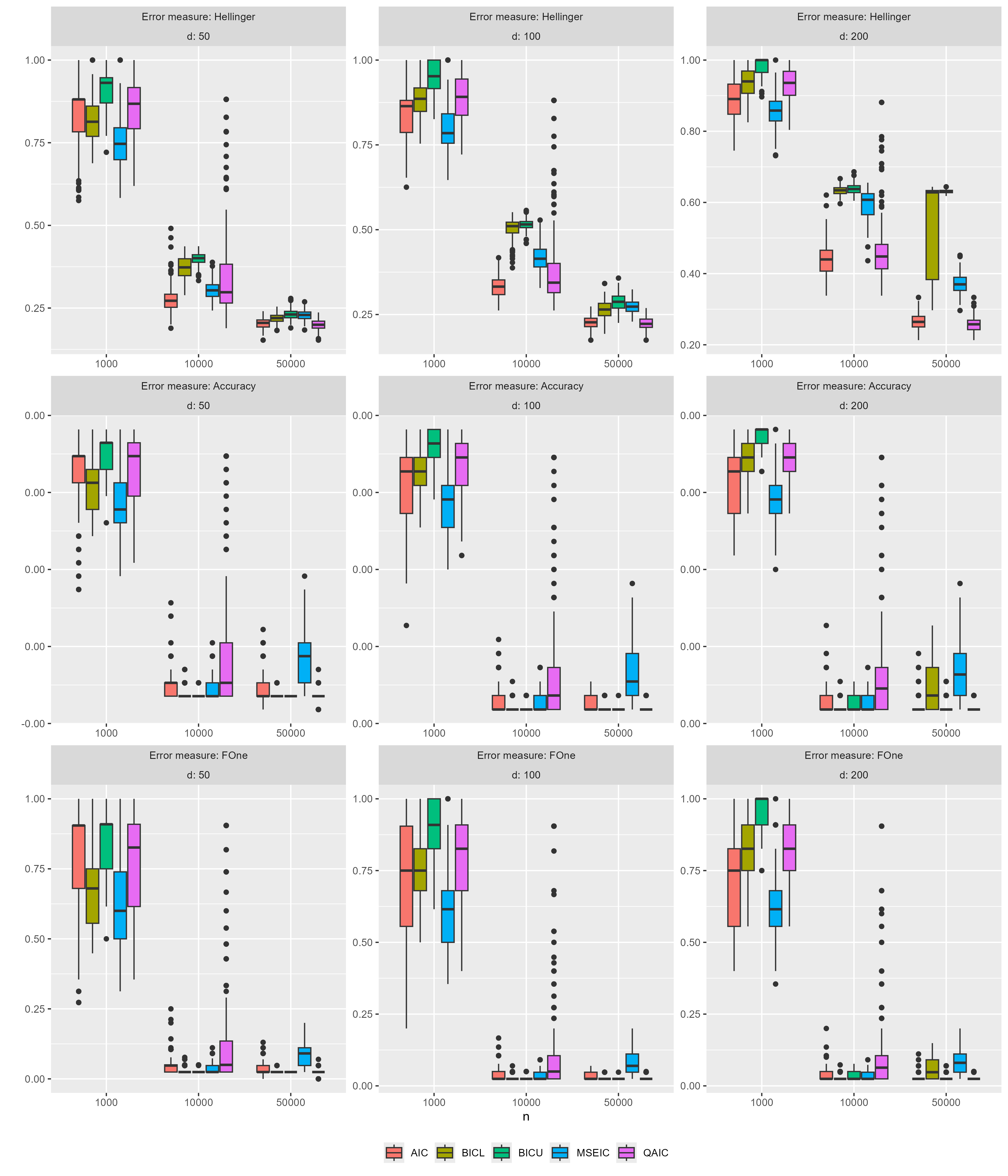
Figure 5: Simulations for asymptotic dependent data with $s^{*}=20$ directions of extremes: From left to the right the dimension increases from $d=50$, $d=100$ to $d=200$. In the top row we use as an error measure the Hellinger distance, in the middle row the Accuracy Error and in the bottom row the $F_{1}$ Error, which are plotted on the $y$-axis against the sample size $n$ on the $x$-axis.

In Figure 5 we can see that the error measures behave similarly. For all $d$ we have an increase in performance across all information criteria as $n$ for most of the information criteria. Also, $\operatorname{MSEIC}$ tends to overfit, when the sample size $n$ is $50000$ and includes more directions than necessary. On the other hand, $\operatorname{AIC}$, $\operatorname{BICU}$ and $\operatorname{QAIC}$ do not exhibit this tendency. Further, $\operatorname{MSEIC}$ performs in comparison to the other information criteria better when the sample size is small. When considering only the Hellinger distance, then the $\operatorname{AIC}$ and $\operatorname{QAIC}$ are superior for $n=10000,50000$, but not for the $F_{1}$ or the accuracy. The influence of an increasing dimension $d$ is modest, as the number of relevant directions is fixed.

References

- Avella-Medina, Davis and Samorodnitsky [2022] {barticle}[author] \bauthor\bsnmAvella-Medina, \bfnmMarco\binitsM., \bauthor\bsnmDavis, \bfnmRichard A.\binitsR. A. and \bauthor\bsnmSamorodnitsky, \bfnmGennady\binitsG. (\byear2022). \btitleKernel PCA for multivariate extremes. \bjournalarXiv: 2211.13172. \endbibitem
- Avella Medina, Davis and Samorodnitsky [2024] {barticle}[author] \bauthor\bsnmAvella Medina, \bfnmMarco\binitsM., \bauthor\bsnmDavis, \bfnmRichard A.\binitsR. A. and \bauthor\bsnmSamorodnitsky, \bfnmGennady\binitsG. (\byear2024). \btitleSpectral learning of multivariate extremes. \bjournalJ. Mach. Learn. Res. \bvolume25. \endbibitem
- Bernard et al. [2013] {barticle}[author] \bauthor\bsnmBernard, \bfnmElsa\binitsE., \bauthor\bsnmNaveau, \bfnmPhilippe\binitsP., \bauthor\bsnmVrac, \bfnmMathieu\binitsM. and \bauthor\bsnmMestre, \bfnmOlivier\binitsO. (\byear2013). \btitleClustering of Maxima: Spatial Dependencies among Heavy Rainfall in France. \bjournalJournal of Climate \bvolume26 \bpages7929-7937. \endbibitem
- Burnham and Anderson [1998] {bbook}[author] \bauthor\bsnmBurnham, \bfnmKenneth P.\binitsK. P. and \bauthor\bsnmAnderson, \bfnmDavid Raymond\binitsD. R. (\byear1998). \btitleModel selection and inference: a practical information theoretic approach. \bpublisherSpringer, \baddressNew York. \endbibitem
- Cavanaugh and Neath [1999] {barticle}[author] \bauthor\bsnmCavanaugh, \bfnmJoseph E.\binitsJ. E. and \bauthor\bsnmNeath, \bfnmAndrew A.\binitsA. A. (\byear1999). \btitleGeneralizing the derivation of the Schwarz information criterion. \bjournalComm. Statist. Theory Methods \bvolume28 \bpages49–66. \endbibitem
- Chautru [2015] {barticle}[author] \bauthor\bsnmChautru, \bfnmEmilie\binitsE. (\byear2015). \btitleDimension reduction in multivariate extreme value analysis. \bjournalElectron. J. Stat. \bvolume9 \bpages383–418. \endbibitem
- Claeskens [2016] {barticle}[author] \bauthor\bsnmClaeskens, \bfnmGerda\binitsG. (\byear2016). \btitleStatistical Model Choice. \bjournalAnnu. Rev. Stat. Appl. \bvolume3 \bpages233-256. \endbibitem
- Clémençon, Huet and Sabourin [2024] {barticle}[author] \bauthor\bsnmClémençon, \bfnmStephan\binitsS., \bauthor\bsnmHuet, \bfnmNathan\binitsN. and \bauthor\bsnmSabourin, \bfnmAnne\binitsA. (\byear2024). \btitleRegular variation in Hilbert spaces and principal component analysis for functional extremes. \bjournalStochastic Process. Appl. \bvolume174 \bpagesPaper No. 104375, 22. \endbibitem
- Cooley and Thibaud [2019] {barticle}[author] \bauthor\bsnmCooley, \bfnmD.\binitsD. and \bauthor\bsnmThibaud, \bfnmE.\binitsE. (\byear2019). \btitleDecompositions of dependence for high-dimensional extremes. \bjournalBiometrika \bvolume106 \bpages587–604. \endbibitem
- Cover [2006] {bbook}[author] \bauthor\bsnmCover, \bfnmThomas M.\binitsT. M. (\byear2006). \btitleElements of information theory. \bpublisherWiley-Interscience. \endbibitem
- Drees and Sabourin [2021] {barticle}[author] \bauthor\bsnmDrees, \bfnmHolger\binitsH. and \bauthor\bsnmSabourin, \bfnmAnne\binitsA. (\byear2021). \btitlePrincipal component analysis for multivariate extremes. \bjournalElectron. J. Stat. \bvolume15 \bpages908–943. \endbibitem
- Duchi et al. [2008] {barticle}[author] \bauthor\bsnmDuchi, \bfnmJohn\binitsJ., \bauthor\bsnmShalev-Shwartz, \bfnmShai\binitsS., \bauthor\bsnmSinger, \bfnmYoram\binitsY. and \bauthor\bsnmChandra, \bfnmTushar\binitsT. (\byear2008). \btitleEfficient projections onto the ball for learning in high dimensions. \bjournalProceedings of the 25th International Conference on Machine Learning \bpages272-279. \endbibitem
- Engelke and Hitz [2020] {barticle}[author] \bauthor\bsnmEngelke, \bfnmSebastian\binitsS. and \bauthor\bsnmHitz, \bfnmAdrien S.\binitsA. S. (\byear2020). \btitleGraphical models for extremes. \bjournalJ. R. Stat. Soc. Ser. B. Stat. Methodol. \bvolume82 \bpages871–932. \bnoteWith discussions. \endbibitem
- Engelke and Ivanovs [2021] {barticle}[author] \bauthor\bsnmEngelke, \bfnmSebastian\binitsS. and \bauthor\bsnmIvanovs, \bfnmJevgenijs\binitsJ. (\byear2021). \btitleSparse structures for multivariate extremes. \bjournalAnnu. Rev. Stat. Appl. \bvolume8 \bpages241–270. \endbibitem
- Engelke and Volgushev [2022] {barticle}[author] \bauthor\bsnmEngelke, \bfnmSebastian\binitsS. and \bauthor\bsnmVolgushev, \bfnmStanislav\binitsS. (\byear2022). \btitleStructure learning for extremal tree models. \bjournalJ. R. Stat. Soc. Ser. B. Stat. Methodol. \bvolume84 \bpages2055–2087. \endbibitem
- Engelke et al. [2024] {barticle}[author] \bauthor\bsnmEngelke, \bfnmSebastian\binitsS., \bauthor\bsnmHentschel, \bfnmManuel\binitsM., \bauthor\bsnmLalancette, \bfnmMichaël\binitsM. and \bauthor\bsnmRöttger, \bfnmFrank\binitsF. (\byear2024). \btitleGraphical models for multivariate extremes. \bjournalhttps://arxiv.org/abs/2402.02187. \endbibitem
- Falk [2019] {bbook}[author] \bauthor\bsnmFalk, \bfnmMichael\binitsM. (\byear2019). \btitleMultivariate extreme value theory and D-norms. \bseriesSpringer Series in Operations Research and Financial Engineering. \bpublisherSpringer, Cham. \endbibitem
- Fomichov and Ivanovs [2023] {barticle}[author] \bauthor\bsnmFomichov, \bfnmV.\binitsV. and \bauthor\bsnmIvanovs, \bfnmJ.\binitsJ. (\byear2023). \btitleSpherical clustering in detection of groups of concomitant extremes. \bjournalBiometrika \bvolume110 \bpages135–153. \endbibitem
- Gissibl and Klüppelberg [2018] {barticle}[author] \bauthor\bsnmGissibl, \bfnmNadine\binitsN. and \bauthor\bsnmKlüppelberg, \bfnmClaudia\binitsC. (\byear2018). \btitleMax-linear models on directed acyclic graphs. \bjournalBernoulli \bvolume24 \bpages2693–2720. \endbibitem
- Gissibl, Klüppelberg and Lauritzen [2021] {barticle}[author] \bauthor\bsnmGissibl, \bfnmNadine\binitsN., \bauthor\bsnmKlüppelberg, \bfnmClaudia\binitsC. and \bauthor\bsnmLauritzen, \bfnmSteffen\binitsS. (\byear2021). \btitleIdentifiability and estimation of recursive max-linear models. \bjournalScand. J. Stat. \bvolume48 \bpages188–211. \endbibitem
- Goix, Sabourin and Clémençon [2017] {barticle}[author] \bauthor\bsnmGoix, \bfnmNicolas\binitsN., \bauthor\bsnmSabourin, \bfnmAnne\binitsA. and \bauthor\bsnmClémençon, \bfnmStephan\binitsS. (\byear2017). \btitleSparse representation of multivariate extremes with applications to anomaly detection. \bjournalJ. Multivariate Anal. \bvolume161 \bpages12–31. \endbibitem
- Haslett and Raftery [1989] {barticle}[author] \bauthor\bsnmHaslett, \bfnmJohn\binitsJ. and \bauthor\bsnmRaftery, \bfnmAdrian E.\binitsA. E. (\byear1989). \btitleSpace-Time Modelling with Long-Memory Dependence: Assessing Ireland’s Wind Power Resource. \bjournalJ. R. Stat. Soc. Ser. C. Appl. Stat. \bvolume38 \bpages1–50. \endbibitem
- Jalalzai and Leluc [2021] {binproceedings}[author] \bauthor\bsnmJalalzai, \bfnmHamid\binitsH. and \bauthor\bsnmLeluc, \bfnmRémi\binitsR. (\byear2021). \btitleFeature Clustering for Support Identification in Extreme Regions. In \bbooktitleProceedings of the 38th International Conference on Machine Learning (\beditor\bfnmMarina\binitsM. \bsnmMeila and \beditor\bfnmTong\binitsT. \bsnmZhang, eds.). \bseriesProceedings of Machine Learning Research \bvolume139 \bpages4733–4743. \bpublisherPMLR. \endbibitem
- Janßen and Wan [2020] {barticle}[author] \bauthor\bsnmJanßen, \bfnmAnja\binitsA. and \bauthor\bsnmWan, \bfnmPhyllis\binitsP. (\byear2020). \btitle-means clustering of extremes. \bjournalElectron. J. Stat. \bvolume14 \bpages1211-1233. \endbibitem
- Meyer and Wintenberger [2021] {barticle}[author] \bauthor\bsnmMeyer, \bfnmNicolas\binitsN. and \bauthor\bsnmWintenberger, \bfnmOlivier\binitsO. (\byear2021). \btitleSparse regular variation. \bjournalAdv. in Appl. Probab. \bvolume53 \bpages1115–1148. \endbibitem
- Meyer and Wintenberger [2023] {barticle}[author] \bauthor\bsnmMeyer, \bfnmNicolas\binitsN. and \bauthor\bsnmWintenberger, \bfnmOlivier\binitsO. (\byear2023). \btitleMultivariate Sparse Clustering for Extremes. \bjournalJ. Amer. Statist. Assoc. \bpages1-12. \endbibitem
- Ouimet [2021] {barticle}[author] \bauthor\bsnmOuimet, \bfnmFrédéric\binitsF. (\byear2021). \btitleA precise local limit theorem for the multinomial distribution and some applications. \bjournalJ. Statist. Plann. Inference \bvolume215 \bpages218-233. \endbibitem
- Powers [2008] {barticle}[author] \bauthor\bsnmPowers, \bfnmDavid\binitsD. (\byear2008). \btitleEvaluation: From Precision, Recall and F-Factor to ROC, Informedness, Markedness and Correlation. \bjournalMach. Learn. Technol. \bvolume2. \endbibitem
- Resnick [1987] {bbook}[author] \bauthor\bsnmResnick, \bfnmS. I.\binitsS. I. (\byear1987). \btitleExtreme Values, Regular Variation, and Point Processes. \bpublisherSpringer. \endbibitem
- Resnick [2007] {bbook}[author] \bauthor\bsnmResnick, \bfnmS. I.\binitsS. I. (\byear2007). \btitleHeavy-Tail Phenomena: Probabilistic and Statistical Modeling. \bpublisherSpringer. \endbibitem
- Rohrbeck and Cooley [2023] {barticle}[author] \bauthor\bsnmRohrbeck, \bfnmChristian\binitsC. and \bauthor\bsnmCooley, \bfnmDaniel\binitsD. (\byear2023). \btitleSimulating flood event sets using extremal principal components. \bjournalAnn. Appl. Stat. \bvolume17 \bpages1333–1352. \endbibitem
- Schwarz [1978] {barticle}[author] \bauthor\bsnmSchwarz, \bfnmGideon\binitsG. (\byear1978). \btitleEstimating the dimension of a model. \bjournalAnn. Statist. \bvolume6 \bpages461–464. \endbibitem
- Simpson, Wadsworth and Tawn [2020] {barticle}[author] \bauthor\bsnmSimpson, \bfnmE. S.\binitsE. S., \bauthor\bsnmWadsworth, \bfnmJ. L.\binitsJ. L. and \bauthor\bsnmTawn, \bfnmJ. A.\binitsJ. A. (\byear2020). \btitleDetermining the dependence structure of multivariate extremes. \bjournalBiometrika \bvolume107 \bpages513–532. \endbibitem
- StatLib---Datasets-Archive [2023] {bmisc}[author] \bauthor\bsnmStatLib---Datasets-Archive (\byear2023). \btitleWind. \bhowpublishedhttp://lib.stat.cmu.edu/datasets/wind.data, accessed October 26, 2023. \endbibitem

References

- Fujikoshi, Ulyanov and Shimizu [2010] {bbook}[author] \bauthor\bsnmFujikoshi, \bfnmYasunori\binitsY., \bauthor\bsnmUlyanov, \bfnmVladimir Vladimirovič\binitsV. V. and \bauthor\bsnmShimizu, \bfnmRyoichi\binitsR. (\byear2010). \btitleMultivariate statistics: high-dimensional and large-sample approximations. \bpublisherWiley. \endbibitem
- Hille [1964] {bbook}[author] \bauthor\bsnmHille, \bfnmEinar\binitsE. (\byear1964). \btitleAnalysis 1. \bpublisherBlaisdell Publ. Co. \endbibitem
- Horn and Johnson [2013] {bbook}[author] \bauthor\bsnmHorn, \bfnmRoger A.\binitsR. A. and \bauthor\bsnmJohnson, \bfnmCharles R.\binitsC. R. (\byear2013). \btitleMatrix analysis, \bedition2. ed., 1. publ. ed. \bpublisherCambridge Univ. Press. \endbibitem
- Meyer and Wintenberger [2020] {barticle}[author] \bauthor\bsnmMeyer, \bfnmNicolas\binitsN. and \bauthor\bsnmWintenberger, \bfnmOlivier\binitsO. (\byear2020). \btitleTail inference for high-dimensional data. \bjournalarXiv: 2007.11848v1. \endbibitem
- Meyer and Wintenberger [2023] {barticle}[author] \bauthor\bsnmMeyer, \bfnmNicolas\binitsN. and \bauthor\bsnmWintenberger, \bfnmOlivier\binitsO. (\byear2023). \btitleMultivariate Sparse Clustering for Extremes. \bjournalJ. Amer. Statist. Assoc. \bpages1-12. \endbibitem