Quantifying non-Markovianity via local quantum Fisher information

Abstract

Non-Markovian dynamics in open quantum systems arise when the system’s evolution is influenced by its past interactions with the environment. Here, we present a novel metric for quantifying non-Markovianity based on local quantum Fisher information (LQFI). The proposed metric offers a distinct perspective compared to existing measures, providing a deeper understanding of information flow between the system and its environment. By comparing the LQFI-based measure to the LQU-based measure, we demonstrate its effectiveness in detecting non-Markovianity and its ability to capture the degree of non-Markovian behavior in various quantum channels. Furthermore, we show that a positive time derivative of LQFI signals the flow of information from the environment to the system, providing a clear interpretation of non-Markovian dynamics. Finally, the computational efficiency of the LQFI-based measure makes it a practical tool for characterizing non-Markovianity in diverse physical systems.

Keywords: Local quantum Fisher information, Open quantum systems, Markoian and non-Markovian regions.

I Introduction

Over recent years, quantum mechanics has not been merely a fundamental theory restricted to the background theory but has also penetrated the experimental level through many quantum technological revolutions. These technologies are motivated through the prospect of quantum computers and quantum communications [1, 2, 3, 4]. Unfortunately, they still suffer from unavoidable interactions with the environment, leading to a lack of quantum properties due to decoherence phenomena [5, 6, 7]. All related questions have been addressed. The practical problems of quantum device engineering required for the developing areas of technology and quantum computing have also been addressed, or at least investigated, in the theory of open quantum systems (OQSs). As far as we know, the development of these quantum systems began with optical quantum systems, characterised by a generally weak and unstructured system-environment coupling [8, 9, 10, 11]. In such weak couplings, it is often reasonable be assumed to be memoryless, meaning that not information flows back into the system later. In such situations, the Markov and Born approximations hold, which allows us to obtain the time-local master equation within the OQS in the Lindblad form [12, 13]. If the dynamics are of a Markovian nature, the loss of information will only occur in one direction flow of information from the system to the environment. Conversely, non-Markovian dynamics presents more interesting phenomena due to the memory effect and has been used in various quantum processes. Thus, the problem of the characterisation of our non-Markovian effect quickly became a major topic in the theory of open quantum dynamics [14, 15, 16, 17]. Non-Markovianity has shown significant potential applications in quantum information processing. These include the preparation of stable entangled states [18], provision of a quantum resource [19], improvement of achievable resolution in quantum metrology [20], acceleration of quantum evolution [21, 22] and more. Theoretically, several measures and non-Markovian witnesses have been proposed, but they may not all precisely coincide when it comes to detecting non-Markovianity. Currently, we possess multiple closely linked yet conceptually different definitions of non-Markovianity. Among the measures are those grounded in the semigroup property [23, 24], trace distance between quantum states [25, 26], fidelity [27], divisibility [28, 29], quantum Fisher information flow [30, 31], quantum capacity [32], quantum mutual information [33], relative entropy of coherence [34] and local quantum uncertainty [35, 36]. A universally accepted characterization for quantum non-Markovianity in OQSs is currently unavailable and may not exist.

Recent advances in experimental techniques for manipulating and controlling system-environment interactions have generated considerable enthusiasm for characterizing and quantifying non-Markovian dynamics. This interest extends to exploring potential applications in evolutionary quantum technologies that exhibit robustness against environmentally-induced decoherence. Recently, two computational measures of the nature of quantum correlations have been proposed. One quantifier is the local quantum uncertainty (LQU), which quantifies the minimum uncertainty resulting from applying local measurements to a subset of the quantum state using the Wigner-Yanase information concept [37, 38]. One of the notable advantages of the LQU is the ability to calculate any qubit-qudit system. The other is the local quantum Fisher information (QFI), which plays a central role in quantifying the information available through a local observable within a quantum system. This measure is defined as the minimisation of the QFI associated with a local observable, indicating the maximum information achievable within one of the subsystems [39]. However, LQFI has considerable potential as a tool for comprehending effects of quantum correlations extending beyond entanglement and for enhancing the precision of quantum estimation protocols [40]. In addition to its importance as a quantifier of quantum correlation, it introduced LQU to new methods for detecting non-Markovianity for an OQS [35]. Certainly, a fundamental inquiry arises regarding the applicability of LQFI in delineating the intricate quantum systems exhibiting non-Markovian characteristics?

The search for detecting non-Markovianity in OQSs has led to various approaches, including the use of LQU and other metrics as proposed in [35]. Our LQFI-based approach introduces a simple and mathematically tractable measure of non-Markovianity. Focusing on a bipartite system $AB$, where $A$ is the primary system interacting with the environment and $B$ is the ancilla, we assess the LQFI by applying local unitary operations to the ancilla, effectively using it as a measuring apparatus. In this context, the non-Markovianity of the system evolution is quantified through the evaluation of non-monotonic tendencies of the LQFI. Furthermore, it is imperative to highlight that the non-Markovianity measure derived through LQFI exhibits a qualitative consistency with several other established measures used in the context of OQSs. In our investigation, we have shown that this LQFI-based measure is consistent with metrics based on the divisibility concept, LQU, relative entropy and quantum mutual information.

The structure of this manuscript unfolds as follows: Section II begins with a review of the concept of local quantum Fisher information and some of its properties. Following this, a non-Markovianity measure based on LQFI for OQSs is introduced. Moving on to Section III, we present illustrative examples to demonstrate the practical utility of this measure, juxtaposing it with the based-LQU measure. Finally, our findings are summarised in Section IV.

II Measuring non-Markovianity via local quantum Fisher information

Local quantum Fisher information is a fundamental concept in quantum information theory and quantum estimation theory. Recently, it has emerged as an important measure of non-classical correlations. For a given quantum state $\varrho^{AB}=\sum_{m}|{\phi_{m}}\rangle\langle{\phi_{m}}|$ with $h_{m}\geq 1$ and $\sum_{m}h_{m}=1$, the LQFI associated with the local evolution generated by $L_{A}\otimes I_{B}$ can be expressed as [39, 41]

$$\mathcal{F}\left(\varrho^{AB},L_{A}\right)=\frac{1}{2}\sum_{m\neq n}\frac{\left(h_{m}-h_{n}\right)^{2}}{h_{m}+h_{n}}\arrowvert\langle{\phi_{m}}|L_{A}\otimes I_{B}|{\phi_{n}}\rangle\arrowvert^{2}.$$ (1)

The expresion above can be equivalently reformulated as

$$\mathcal{F}\left(\varrho^{AB},L_{A}\right)=Tr\left\{\varrho_{AB}L_{A}^{2}\right\}-\sum_{m\neq n}\frac{2h_{m}h_{n}}{h_{m}+h_{n}}\arrowvert\langle{\phi_{m}}|L_{A}|{\phi_{n}}\rangle\arrowvert^{2}.$$ (2)

The local quantum information Fisher $\mathcal{Q}\left(\varrho^{AB}\right)$ quantifies the quantum correlations. It is defined as the minimum quantum Fisher information overall local Hamiltonians $L_{A}$ acting in the subspace of party $A$ of the bipartite system $AB$, i.e.,

$$\mathcal{Q}\left(\varrho^{AB}\right)=\underset{L_{A}}{\text{min}}\mathcal{F}\left(\varrho^{AB},L_{A}\right).$$ (3)

The local Hamiltonian in its typical form is represented as $L_{a}=\vec{\sigma}.\vec{v}$, with $\arrowvert\vec{v}\arrowvert=1$ and $\vec{\sigma}=\left(\sigma_{1},\sigma_{2},\sigma_{3}\right)$ the Pauli matrices, one has $Tr\left(\varrho^{AB},L_{A}^{2}\right)=1$, and the second term in Eq.(2) can be expressed as

$$\sum_{m\neq n}\frac{2h_{m}h_{n}}{h_{m}+h_{n}}\arrowvert\langle{\phi_{m}}|L_{A}|{\phi_{n}}\rangle\arrowvert^{2}=\vec{v}^{\dagger}.\mathcal{S}.\vec{v},$$ (4)

where the components of the symmetric matrix $\mathcal{S}$ are given by

$$\mathcal{S}_{kl}=\sum_{m\neq n}\sum\limits_{k,l=1}^{3}\frac{2h_{m}h_{n}}{h_{m}+h_{n}}\langle{\phi_{m}}|\sigma_{k}\otimes I|{\phi_{n}}\rangle\langle{\phi_{n}}|\sigma_{l}\otimes I|{\phi_{m}}\rangle.$$ (5)

To minimize $\mathcal{F}$, it’s essential to maximize the expression $\vec{v}^{\dagger}.\mathcal{S}.\vec{v}$ over all unit vectors. This maximum value corresponds to the maximum eigenvalue of $\mathcal{S}$. Therefore, the minimum value of the LQFI is

$$\mathcal{Q}\left(\varrho^{AB}\right)=1-\eta_{\max}\left(\mathcal{S}\right),$$ (6)

where $\eta_{\max}\left(\mathcal{S}\right)$ is the maximum eigenvalue of the real symmetric matrix $\mathcal{S}$. LQFI has several properties that make it a valuable measure of quantum correlations [39]:

First, the $\mathcal{Q}\left(\varrho^{AB}\right)$ is preserved under unitary transformations $U$, i.e., $\mathcal{Q}\left(\left(U^{A}\otimes U^{B}\right)\varrho^{AB}\left(U^{A}\otimes U^{B}\right)^{\dagger}\right)=\mathcal{Q}\left(\varrho^{AB}\right)$.

Second, $\mathcal{Q}\left(\varrho^{AB}\right)$ is non-increasing (contractive) under any local completely positive trace preserving (l-CPTP) map $\Phi$ on party, i.e. $\mathcal{Q}\left(\varrho^{AB}\right)\geq\mathcal{Q}\left(\Phi\varrho^{AB}\right)$. For a composite quantum system there exists a minor extension of this property $Q\left(\varrho^{AB}\right)\geq Q\left(\left(I^{A}\otimes\Phi^{B}\right)\varrho^{AB}\right)$.

By a simple demonstration, we show the extension of the last property on composite systems , we have $\Phi^{A}\left(\varrho^{A}\right)=\sum\limits_{n}\lambda_{n}U_{n}\varrho^{A}U_{n}^{\dagger}$ is a random unitary channel. $U_{n}$ are unitary operators on $L_{A}$, and $\lambda_{n}$ satisfy $\sum_{n}\lambda_{n}=1$, $0\leq\lambda_{n}\leq 1$. Then we have

$$\mathcal{F}\left(\left(I^{A}\otimes\Phi^{B}\right)\varrho^{AB},L_{A}\right)\leq\mathcal{F}\left(\varrho^{AB},L_{A}\right).$$ (7)

So,

$$\mathcal{Q}\left(\varrho^{AB}\right) =\min_{L_{A}}\mathcal{F}\left(\varrho^{AB},L_{A}\right)$$

$$\geq\min_{L_{A}}\mathcal{F}\left(\left(I^{A}\otimes\Phi^{B}\right)\varrho^{AB},L_{A}\right)$$

$$=\mathcal{Q}\left(\left(I^{A}\otimes\Phi^{B}\right)\varrho^{AB}\right).$$ (8)

The last property of LQFI (monotonicity) is paramount in underpinning the formulation of the novel measure of non-Markovianity proposed. This foundational principle is intimately linked with the concept of divisibility . The evolution of a quantum dynamical map, denoted as $\left\{\Phi\right\}$, over time. A quantum dynamical map $\left\{\Phi\right\}$ is divisible if and only if it meets

$$\Phi_{t}=\Phi_{t,v}\Phi_{v},$$ (9)

with $\Phi_{t,v}$ signifies completely positive map for any $t>v\geq 0$. In Refs[14, 15, 16, 17], all divisible dynamics are defined as Markovian, while non-divisible dynamics are defined as non-Markovian.

For Markovian dynamics, the evolution is described by a divisible lCPTP map $\Phi$. The composite dynamics of the entire system $\varrho^{AB}\left(t\right)$ is given by the Jamiolkowski-Choi isomorphism [42]

$$\varrho^{AB}\left(t\right)=\left(I^{A}\otimes\Phi_{t}^{B}\right)\varrho^{AB}$$ (10)

where $I^{A}$ represents the identity operation on the ancillary subsystem A. We have,

$$\mathcal{Q}\left(\varrho^{AB}\left(t\right)\right) =\mathcal{Q}\left(\left(I^{A}\otimes\Phi_{t}\right)\varrho^{AB}\right)$$

$$=\mathcal{Q}\left(\left(I^{A}\otimes\Phi_{t,v}\Phi_{v}\right)\varrho^{AB}\right)$$

$$=\mathcal{Q}\left(\left(I^{A}\otimes\Phi_{t,v}\right)\varrho^{AB}\left(v\right)\right)$$

$$\leq\mathcal{Q}\left(\varrho^{AB}\left(v\right)\right).$$ (11)

The monotonicity of the local quantum Fisher information under local operations lays the groundwork for understanding the dynamics of quantum systems. Consequently, the LQFI, $\mathcal{Q}\left(\varrho^{AB}\left(t\right)\right)$ is non-increasing monotone with increasing time. Hence, which implies that $\frac{d\mathcal{Q}\left(\varrho^{AB}\left(t\right)\right)}{dt}\leq 0$ for any Markovian dynamics [33, 35]. In other words, the appearance of non-Markovianity of a dynamical process is implied by the breaking of this monotonicity, i.e.,

$$\frac{d\mathcal{Q}\left(\varrho^{AB}\left(t\right)\right)}{dt}>0.$$ (12)

Consequently, we develope a measure of non-Markovianity

$$\mathcal{N}^{LQFI}\left(\Phi\right)=\max_{\varrho^{AB}\left(0\right)}\int_{\mathcal{D}_{\mathcal{Q}}\left(t\right)>0}\mathcal{D}_{\mathcal{Q}}\left(t\right)dt,$$ (13)

where $\mathcal{D}_{\mathcal{Q}}\left(t\right)=\frac{d\mathcal{Q}\left(\varrho^{AB}\left(t\right)\right)}{dt}$ with $\varrho^{AB}\left(t\right)=\left(I^{A}\otimes\Phi_{t}^{B}\right)\varrho^{AB}\left(0\right)$, $\varrho^{AB}\left(0\right)$ is a maximally entangled state for bipartite systems AB. In this context Numerically, the above equation (13) can also be written as

$$\mathcal{N}^{LQFI}\left(\Phi\right)=\max_{\varrho^{AB}\left(0\right)}\sum\limits_{k}\left[\mathcal{Q}\left(x_{f}^{k}\right)-\mathcal{Q}\left(x_{i}^{k}\right)\right],$$ (14)

where the time intervals $\left[x_{i}^{k},x_{f}^{k}\right]$ represent all regions where $\mathcal{D}_{\mathcal{Q}}\left(t\right)>0$, indicating deviations from non-Markovian dynamics. The maximization is performed over all pairs of initial states. To accurately compute this measure, it is imperative to determine the cumulative increase of the local quantum Fisher information within each time interval $\left[x_{i}^{k},x_{f}^{k}\right]$ and then aggregate the contributions from all such intervals.

The local quantum Fisher information connection to quantum metrology further enhances its relevance, as it is directly linked to the precision of parameter estimation in quantum systems. This makes LQFI particularly useful in scenarios where non-Markovianity impacts measurement precision. Furthermore, LQFI offers greater mathematical flexibility, enabling it to be adapted to various types of interactions and dynamics, making it a more versatile tool across different scenarios. In contrast, LQU may not provide the same level of precision or adaptability, especially in systems with complex dynamics. In quantum metrology, quantum Fisher information and skew information satisfy the following inequality relation [41]

$$\mathcal{I}\left(\varrho,L\right)\leq\mathcal{F}\left(\varrho,L\right)\leq 2\mathcal{I}\left(\varrho,L\right)$$ (15)

Where

$$\mathcal{F}\left(\varrho,L\right)=\frac{1}{2}\sum\limits_{m,n}\left(1+\frac{2\sqrt{h_{m}h_{n}}}{h_{m}+h_{n}}\right)\left(\sqrt{h_{m}}-\sqrt{h_{n}}\right)^{2}\arrowvert\langle{\phi_{m}}|L|{\phi_{n}}\rangle\arrowvert^{2},$$ (16)

$$\mathcal{I}\left(\varrho,L\right)=\frac{1}{2}\sum\limits_{m,n}\left(\sqrt{h_{m}}-\sqrt{h_{n}}\right)^{2}\arrowvert\langle{\phi_{m}}|L|{\phi_{n}}\rangle\arrowvert^{2}.$$ (17)

Correspondingly, the derivatives of the QFI $\mathcal{F}\left(\varrho,L\right)$ can be obtained as

$$\frac{d\mathcal{F}\left(\varrho,L\right)}{dt}=\sum_{m,n}\Bigg{[} \left(1+\frac{2\sqrt{h_{m}h_{n}}}{h_{m}+h_{n}}\right)\frac{d\mathcal{I}\left(\varrho,L\right)}{dt}$$

$$+\mathcal{I}\left(\varrho,L\right)\frac{d}{dt}\left(1+\frac{2\sqrt{h_{m}h_{n}}}{h_{m}+h_{n}}\right)\Bigg{]},$$ (18)

where

$$\frac{d}{dt}\left(1+\frac{2\sqrt{h_{m}h_{n}}}{p_{m}+p_{n}}\right)=\frac{\dot{h}_{m}h_{n}\left(1-2h_{m}\right)+h_{m}\dot{h}_{n}\left(1-2h_{n}\right)}{\left(h_{m}+h_{n}\right)^{2}\sqrt{h_{m}h_{n}}},$$

with $0\leq h_{m,n}\leq 1$ and $0\leq\dot{h}_{m,n}\leq 1$, we find that

$$0\leq\frac{d}{dt}\left(1+\frac{2\sqrt{h_{m}h_{n}}}{h_{m}+h_{n}}\right)\leq\frac{1}{2}.$$ (19)

By of Eq. 18 and Eq. 19 we obtain the new inequality relation

$$\frac{d\mathcal{I}\left(\varrho,L\right)}{dt}\leq\frac{d\mathcal{F}\left(\varrho,L\right)}{dt}\leq 2\frac{d\mathcal{I}\left(\varrho,L\right)}{dt}$$ (20)

Due to the relationship between the derivatives of the skew information and the derivatives of the QFI 20, the above inequality relation is reduced to

$$\frac{d\mathcal{U}\left(\varrho\right)}{dt}\leq\frac{d\mathcal{Q}\left(\varrho\right)}{dt}\leq 2\frac{d\mathcal{U}\left(\varrho\right)}{dt}$$ (21)

A regime is classified as non-Markovian if $\frac{d\mathcal{X}\left(\varrho\right)}{dt}>0$, with $\mathcal{X}\equiv\left(\mathcal{U},\mathcal{Q}\right)$.

$$\mathcal{N}^{LQU}\leq\mathcal{N}^{LQFI}\leq 2\mathcal{N}^{LQU}$$ (22)

III Applications

In this section, we explore several applications of our measure for evaluating non-Markovian processes. By examining these examples, we aim to elucidate the effectiveness of our measure in characterizing quantum dynamical systems.

III.1 Phase damping channel

In this section, our primary focus revolves around the examination and evaluation of the proposed non-Markovianity procedure. Specifically, our objective is to contrast the measure of non-Markovianity based on LQU with our measure (LQFI-based). To provide a concrete context for this analysis, we delve into the typical model depicting a single-qubit dephasing channel. To further elucidate this model, we present the Hamiltonian governing the interaction between a single-qubit and a thermal reservoir [5]

$$H=\omega_{0}\sigma_{z}+\sum\limits_{i}\omega_{i}a_{i}a_{i}^{\dagger}+\sum\limits_{i}\left(g_{i}\sigma_{z}a_{i}+g_{i}^{*}\sigma_{z}a_{i}^{\dagger}\right),$$ (23)

where $\omega_{0}$ denotes the qubit resonant transition frequency, while $a_{i}\left(a_{i}^{\dagger}\right)$ represents the annihilation (creation) operators, The frequency of the ith reservoir mode is denoted by $\omega_{i}$, and $g_{i}$ signifies the reservoir-qubit coupling constant associated with each mode. We consider the scenario where a qubit is subjected to non-Markovian phase-damping noise. The dynamic evolution of the system can be succinctly expressed in the form of the master equation

$$\dot{\varrho}\left(t\right)=\gamma\left(t\right)\left(\sigma_{z}\varrho\left(t\right)\sigma_{z}-\varrho\left(t\right)\right).$$ (24)

The dynamical map that governs the dephasing channel acting on a single-qubit system described by the density operator can be represented as follows

$$\varrho\left(t\right)=\Phi_{t}\varrho\left(0\right)=\begin{pmatrix}a&&P\left(t\right)b\\ P\left(t\right)c&&d\end{pmatrix},$$ (25)

where $P\left(t\right)=\exp\left(-2\Lambda\left(t\right)\right)$ with $\Lambda\left(t\right)=\int_{0}^{t}\gamma\left(v\right)dv$, the decoherence rate is given by the relation for a zero-temperature reservoir with spectral density $J\left(\omega\right)$ [5, 43]

$$\gamma\left(t\right)=\int J\left(\omega\right)\frac{\sin\left(\omega t\right)}{\omega}d\omega.$$ (26)

For initial state $\varrho^{AB}\left(0\right)=|{\psi}\rangle^{AB}\langle{\psi}|$, the total density operator is

$$\varrho^{AB}\left(t\right)=\left(I^{A}\otimes\Phi_{t}^{B}\right)\varrho^{AB}\left(0\right)=\frac{1}{2}\begin{pmatrix}1&&0&&0&&P\left(t\right)\\ 0&&0&&0&&0\\ 0&&0&&0&&0\\ P\left(t\right)&&0&&0&&1\end{pmatrix},$$ (27)

where $|{\psi}\rangle=\frac{1}{\sqrt{2}}\left(|{00}\rangle+|{11}\rangle\right)$. To compute the explicit expression of the LQFI,one must first calculate the elements of the matrix $\mathcal{S}$. Based on equation 5. It is verified that all elements are equal to zero except $\mathcal{S}_{33}$, which is written as follows $1-P\left(t\right)^{2}$. Thus, in this scenario, the LQFI is represented as

$$\mathcal{Q}\left(\varrho^{AB}\left(t\right)\right)=P\left(t\right)^{2},$$ (28)

and

$$\mathcal{D}_{\mathcal{Q}}\left(t\right)=-4\gamma\left(t\right)P\left(t\right)^{2}.$$ (29)

After thorough calculations and analyses, we have derived the explicit formulation of the non-Markovianity measure $\mathcal{N}^{LQFI}\left(\Phi_{t}\right)$ as

$$\mathcal{N}^{LQFI}\left(\Phi_{t}\right) =-\int_{\mathcal{D}_{\mathcal{Q}}\left(t\right)>0}4\gamma\left(t\right)P\left(t\right)^{2}dt$$ (30)

$$=-\int_{\gamma\left(t\right)<0}4\gamma\left(t\right)P\left(t\right)^{2}dt.$$ (31)

Interestingly, this condition $\mathcal{N}^{LQFI}\left(\Phi_{t}\right)>0$ is analogous to $\gamma\left(t\right)<0$, which is consistent with both the measures based on the quantum trace distance, quantum mutual information, and local quantum uncertainty [33, 35].

We consider a reservoir spectral density defined by the expression $J(\omega)=(\omega/\omega_{c})^{s}e^{-\omega/\omega_{c}}$, where $\omega_{c}$ is the reservoir cutoff frequency and $s$ is the ohmicity parameter. The parameter $s$ allows for the transition between different reservoir types: sub-Ohmic for $s<1$, Ohmic for $s=1$, and super-Ohmic for $s>1$. An analytical expression can be found for $\gamma\left(t\right)$ at zero temperature

$$\gamma\left(t\right)=\frac{\omega_{c}\Gamma\left[s\right]\sin\left(\arctan\left(\omega_{c}t\right)\right)}{\left(1+\left(\omega_{c}t\right)^{2}\right)^{s/2}},$$ (32)

where $\Gamma\left[x\right]$ the Euler gamma function.

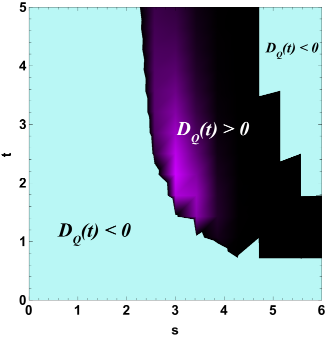
Figure 1: The behaviors of $\mathcal{D}_{\mathcal{Q}}\left(t\right)$ vs time $t$ and ohmicity parameter $s$ for a phase damping channel.

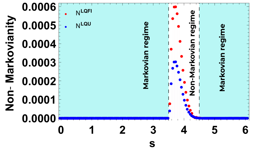
Figure 2: Non-Markovianity $\mathcal{N}^{LQFI}$, $\mathcal{N}^{LQU}$ for the amplitude damping channel as a function of the $s$.

The local quantum Fisher information increases for those times for which $\gamma\left(t\right)<0$, i.e., we will obtain $\mathcal{D}_{\mathcal{Q}}\left(t\right)>0$ for those times. This situation is demonstrated in Fig.(1) for a phase damping channel. The aspect of negative indicates a violation of the divisibility property 9 and the monotonicity. In this Fig.2, we compare our measure $\mathcal{N}^{LQFI}$ (red line) with another quantifier of non-Markovianity $\mathcal{N}^{LQU}$ (Blue line) for a phase-damping channel with an ohmic spectral density. The dashed region, corresponding to $\mathcal{D}_{\mathcal{Q}}>0$, represents the Markovian regime, characterized by $\mathcal{N}=0$ for both measures of non-Markovianity ($\mathcal{N}^{LQFI}$, $\mathcal{N}^{LQU}$) (The zone colored by light blue). We find that the non-Markovian regime exists in the super-ohmic region, $s>3.5$. The behavior of the measures $\mathcal{N}^{LQFI}$ and $\mathcal{N}^{LQU}$ is remarkably similar, showing an initial increase followed by a subsequent decrease as $s$ increases, disappearing at $s<4.5$. Furthermore, it is evident from the results depicted in Fig. 2 that the degree of non-Markovianity, as measured by the measure based on LQFI, is greater than that obtained by the measure based on LQU. This observation aligns with the inequality 22, surpasses that measured by $N^{LQU}$. This result conforms to the inequality 22, that says that the degree of non-Markovainity measured by $\mathcal{N}^{LQFI}$ is greater than the degree of non-Markovainity measured by $\mathcal{N}^{LQU}$.

III.2 Amplitude damping channel

Here, we demonstrate how our measure could be calculated through a typical quantum process. We consider on typical quantum scenario where system B is initially correlated with device A, represented by a two-level (qubit) system [44]. Additionally, the apparatus is in contact with a zero-temperature reservoir, with the primary effect being the introduction of an amplitude damping process solely on the apparatus A. This is a phenomenon that can be aptly described by the following Hamiltonian expression [5].

$$H=\omega_{0}\sigma_{+}\sigma_{-}+\sum\limits_{i}\omega_{i}b_{i}^{\dagger}b_{i}+\sum\limits_{i}\left(g_{i}b_{i}\sigma_{+}+g_{i}^{*}b_{i}^{\dagger}\sigma_{-}\right)$$ (33)

where $\sigma_{+}\left(\sigma_{-}\right)$ represents the raising (lowering) Pauli operator. Its associated dynamics is described using a master equation is

$$\dot{\varrho}\left(t\right)=- \frac{i}{2}h\left(t\right)\left[\sigma_{+}\sigma_{-},\varrho\left(t\right)\right]+$$

$$\gamma\left(t\right)\left[\sigma_{-}\varrho\left(t\right)\sigma_{+}-\frac{1}{2}\left\{\sigma_{+}\sigma_{-},\varrho\left(t\right)\right\}\right],$$ (34)

with

$$h\left(t\right)=-2\mathrm{Im}\frac{\dot{\mathfrak{R}\left(t\right)}}{\mathfrak{R}\left(t\right)},$$ (35)

$$\gamma\left(t\right)=-2\mathrm{Re}\frac{\dot{\mathfrak{R}\left(t\right)}}{\mathfrak{R}\left(t\right)}=-\frac{2}{\arrowvert\mathfrak{R}\left(t\right)\arrowvert}\frac{d}{dt}\arrowvert\mathfrak{R}\left(t\right)\arrowvert,$$ (36)

where $\mathfrak{R}\left(t\right)$ check the following integrodifferential equation with the initial condition $\mathfrak{R}\left(0\right)=1$,

$$\dot{\mathfrak{R}}\left(t\right)=-\int_{0}^{t}g\left(t-t_{1}\right)\mathfrak{R}\left(t_{1}\right)dt_{1}$$ (37)

where the two-point reservoir correlation function $g\left(t-t_{1}\right)$ is derived from the Fourier transform of the reservoir spectral density $J\left(w\right)$:

$$g\left(t-t_{1}\right)=\int J\left(\omega\right)\exp\left[i\left(\omega_{0}-\omega\right)\left(t-t_{1}\right)\right]d\omega.$$ (38)

The evolution of the system qubit $\varrho\left(t\right)$ is determined by the dynamical map is given by

$$\varrho\left(t\right)=\Phi\left(t\right)\varrho\left(0\right)=\begin{pmatrix}1-\arrowvert\mathfrak{R}\left(t\right)\arrowvert^{2}d&&\mathfrak{R}^{*}\left(t\right)b\\ \mathfrak{R}\left(t\right)c&&\arrowvert\mathfrak{R}\left(t\right)\arrowvert^{2}d\end{pmatrix}.$$ (39)

We examine only the case where the reservoir spectral density exhibits the Lorentzian distribution [5], i.e.,

$$J\left(\omega\right)=\frac{\gamma_{0}\lambda^{2}}{2\pi\left[\left(\omega-\omega_{c}\right)^{2}+\lambda^{2}\right]}$$ (40)

where $\omega_{c}$ is the central frequency of the distribution, $\lambda$ denotes the width of the Lorentzian, and $\gamma_{0}$ stands for the system-reservoir coupling constant. By solving Eq. 37 with the correlation function, we derive the following [45]

$$\mathfrak{R}\left(t\right)=e^{\frac{-\left(\lambda-i\Delta\right)t}{2}}\left[\cosh\left(\frac{\Omega t}{2}\right)+\frac{\lambda-i\Delta}{2}\sinh\left(\frac{\Omega t}{2}\right)\right]$$ (41)

Where $\Omega=\sqrt{\left(\lambda-i\Delta\right)^{2}-2\gamma_{0}\lambda}$ and $\left(\Delta=\omega_{0}-\omega_{c}\right)$ is the system-reservoir frequency detuning, with $\omega_{0}$ the qubit frequency.
Now, considering the effect of a single-qubit amplitude damping, the resulting time-evolved density matrix can be expressed as:

$$\varrho^{AB}\left(t\right)=\frac{1}{2}\begin{pmatrix}1&&0&&0&&\mathfrak{R}^{*}\left(t\right)\\ 0&&1-\arrowvert\mathfrak{R}\left(t\right)\arrowvert^{2}&&0&&0\\ 0&&0&&0&&0\\ \mathfrak{R}\left(t\right)&&0&&0&&\arrowvert\mathfrak{R}\left(t\right)\arrowvert^{2}\end{pmatrix}$$ (42)

By a simple arithmetic operation, we find that the expression of the LQFI in this system is written as follows

$$\mathcal{S}_{11}=\mathcal{S}_{22}=1-\arrowvert\mathfrak{R}\left(t\right)\arrowvert^{2},$$ (43)

$$\mathcal{S}_{33}=0$$ (44)

The final expression of the LQFI in the following form

$$\mathcal{Q}\left(\varrho^{AB}\left(t\right)\right)=\arrowvert\mathfrak{R}\left(t\right)\arrowvert^{2}$$ (45)

In turn, the derivative of LQFI $\mathcal{Q}\left(\varrho^{AB}\left(t\right)\right)$ can be obtained in the following form

$$\mathcal{D}_{\mathcal{Q}}\left(t\right)=2\arrowvert\mathfrak{R}\left(t\right)\arrowvert\frac{d\arrowvert\mathfrak{R}\left(t\right)\arrowvert}{dt}$$ (46)

Consequently, the measure of non-Markovianity, $\mathcal{N}^{LQFI}\left(\Phi_{t}\right)$, can be expressed as

$$\mathcal{N}^{LQFI}\left(\Phi_{t}\right) =\int_{\frac{d\arrowvert\mathfrak{R}\left(t\right)\arrowvert}{dt}>0}2\arrowvert\mathfrak{R}\left(t\right)\arrowvert\frac{d\arrowvert.\mathfrak{R}\left(t\right)\arrowvert}{dt}dt$$ (47)

$$=\int_{\gamma\left(t\right)<0}-\gamma\left(t\right)\arrowvert\mathfrak{R}\left(t\right)\arrowvert^{2}dt$$ (48)

Evidently, the condition $\mathcal{N}^{LQFI}\left(\Phi_{t}\right)>0$ is equivalent to $\frac{d\arrowvert\mathfrak{R}\left(t\right)\arrowvert}{dt}>0$ or $\gamma\left(t\right)<0$. This is consistent with other measures, such as those based on dynamical divisibility, mutual quantum information and local quantum uncertainty of the amplitude damping channel.

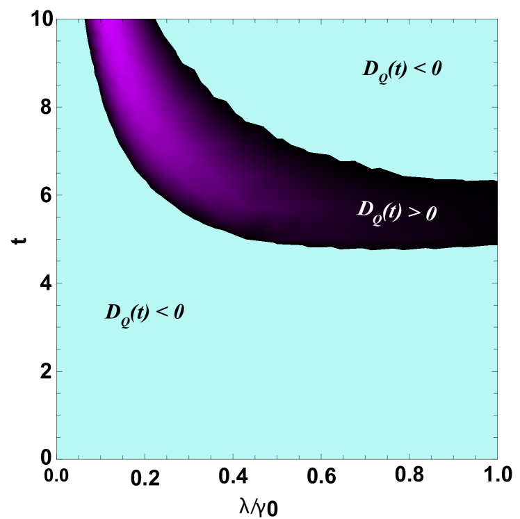
Figure 3: The behaviors of $\mathcal{D}_{\mathcal{Q}}\left(t\right)$ 46 as a function of time $t$ and $\lambda/\gamma_{0}$ for an amplitude damping channel.

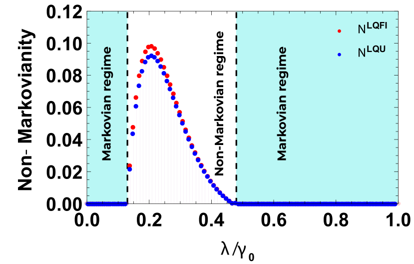
Figure 4: The non-Markovianity $\mathcal{N}^{LQFI}$, $\mathcal{N}^{LQU}$ for the amplitude damping channel as a function of the $\lambda/\gamma_{0}$.

Figure 3 provides a comprehensive visualization of the time derivative of $\mathcal{D}_{\mathcal{Q}}(t)$ as a function of the time and $\lambda/\gamma_{0}$ for the amplitude-damping channel. Remarkably, the observed positivity in certain time intervals of $\mathcal{D}_{\mathcal{Q}}(t)$ indicates that the dynamics of the system are non-Markovian (The zone colored by purple). This departure from Markovian behavior suggests the presence of memory effects within the system evolution, where past states influence future dynamics, a characteristic associated with complex quantum systems.
In this context, Fig.(4) represents of $\mathcal{N}^{LQFI}$ in the phase damping dynamical model, as defined in Eq.(31), the non-Markovian nature is prominently evident within the region $0.18\leq\lambda/\gamma_{0}\leq 0.43$. Intriguingly, the degree of non-Markovianity exhibits a increased behavior, escalating with increasing values of $\lambda/\gamma_{0}$ until reaching a critical point where it peaks. Beyond this peak, a gradual decline ensues until it disappears.

This results, of particular interest for the comparison between $\mathcal{N}^{LQFI}$ and $\mathcal{N}^{LQU}$, revealing intriguing insights into the nature of non-Markovian dynamics. The consistently higher values of $\mathcal{N}^{LQFI}$ compared to $\mathcal{N}^{LQU}$ across various parameter regimes underscore the robustness of the former in capturing dynamics of non-Markovianity. This observation reinforces the theoretical framework laid out by the inequality presented in Eq. 22.

III.3 Depolarizing channel

As a further extension of our methodology, we investigate the non-Markovianity of a non-Markovian depolarising channel. According to Daffer et al [46], they have studied in detail the dynamical characteristics of this system, particularly the total positivity requirements of the map corresponding to a master equation. In this specific model, we can define the time-dependent Hamiltonian using a two-level system subject to random telegraph noise as follows

$$H\left(t\right)=\hbar\sum\limits_{i=1}^{3}\Gamma_{i}\left(t\right)\sigma_{i}$$ (49)

Where $\Gamma_{i}=a_{i}q_{i}\left(t\right)$ be independent random variables and $\sigma_{i}$ be the standard Pauli operators. $q_{i}\left(t\right)$ has a Poisson distribution taking the value $t/2\tau_{i}$, and $a_{i}$ is an independent coin flip random variable taking the value $\pm a_{i}$. The equation of motion for the density operator, corresponding to the time-dependent Hamiltonian given in equation (49), is described by the von Neumann equation

$$\dot{\varrho}\left(t\right)=-i/\hbar\left[H\left(t\right),\varrho\right]=-i\sum_{k}\Gamma_{k}\left(t\right)\left[\sigma_{k},\varrho\right].$$ (50)

The formal solution for this equation is as follows

$$\varrho\left(t\right)=\varrho\left(0\right)-i\int_{0}^{t}\sum_{k}\Gamma_{k}\left(t\right)\left[\sigma_{k},\varrho\right]ds.$$ (51)

The following memory kernel master equation can be obtained by replacing the formal solution Eq. 51 with the von Neumann equation, then executing a stochastic average

$$\dot{\varrho}\left(t\right)=-\int_{0}^{t}\sum_{k}e^{-(t-t^{{}^{\prime}})/\tau_{k}^{2}}\left[\sigma_{k},\left[\sigma_{k},\varrho\left(t^{{}^{\prime}}\right)\right]\right]dt^{{}^{\prime}},$$ (52)

where $<\Gamma_{j}\left(t\right)\Gamma_{k}\left(t^{{}^{\prime}}\right)>=b_{k}^{2}\exp\left(-\arrowvert t-t^{{}^{\prime}}\arrowvert/\tau_{k}\right)\delta_{jk}$ is the memory kernel comes from the correlation functions of random telegraph signal.

As the focus of this study revolves around bipartite systems, it is possible to define the time evolution of initial density operators as [47]

$$\varrho\left(\nu\right)=\sum\limits_{k,l=0}^{3}\left(E_{k}\otimes E_{l}\right)^{\dagger}\varrho\left(0\right)\left(E_{k}\otimes E_{l}\right)$$ (53)

where dimensionless time $\nu=\frac{t}{2\tau}$ , with $\tau_{i}=\tau$. The kraus operators $E_{k,l}=\sqrt{p_{k,l}\left(\nu\right)}\sigma_{k,l}$. The non-negative parameters $p_{k,l}\left(\nu\right)$ are defined by

$$p_{0}\left(\nu\right)=\frac{1}{4}\left[1+\chi_{1}\left(\nu\right)+\chi_{2}\left(\nu\right)+\chi_{3}\left(\nu\right)\right],$$ (54)

$$p_{1}\left(\nu\right)=\frac{1}{4}\left[1+\chi_{1}\left(\nu\right)+\chi_{2}\left(\nu\right)-\chi_{3}\left(\nu\right)\right],$$ (55)

$$p_{2}\left(\nu\right)=\frac{1}{4}\left[1-\chi_{1}\left(\nu\right)+\chi_{2}\left(\nu\right)-\chi_{3}\left(\nu\right)\right],$$ (56)

$$p_{3}\left(\nu\right)=\frac{1}{4}\left[1-\chi_{1}\left(\nu\right)-\chi_{2}\left(\nu\right)+\chi_{3}\left(\nu\right)\right].$$ (57)

where,

$$\chi_{i}\left(\nu\right)=e^{-\nu}\left(\cos\left(\mu_{i}\nu\right)+\sin\left(\mu_{i}\nu\right)/\mu_{i}\right),$$ (58)

with $\mu_{i}=\sqrt{\left(4\kappa_{i}\tau\right)^{2}-1}$, and $k_{i}^{2}=b_{j}^{2}+b_{k}^{2}$ for $i\neq j\neq k,l$. For simplicity, in this study we examine the case where the noise acts in all directions $x$, $y$ and $z$. Particularly, provided that the condition $b_{1}=b_{2}=b_{3}=b$ thus, $\chi_{1}\left(\nu\right)=\chi_{2}\left(\nu\right)=\chi_{3}\left(\nu\right)\equiv\chi\left(\nu\right)$, $p_{1}\left(\nu\right)=p_{2}\left(\nu\right)=p_{3}\left(\nu\right)\equiv\frac{1-\chi\left(\nu\right)}{4}$ and $\chi_{0}\left(\nu\right)=\frac{1+3\chi\left(\nu\right)}{4}$.
To illustrate our discussion, we will initially assume that both qubits are in a maximally mixed state category, as described by the X-structured density operator [15].

$$\varrho\left(0\right)=\frac{1}{4}\left(I\otimes I+\sum\limits_{i=1}^{3}r_{i}\sigma_{i}\otimes\sigma_{i}\right)$$ (59)

In which the correlation parameters satisfy the conditions $0\leq\arrowvert r_{i}\arrowvert\leq 1$ . For simplicity, we take $\arrowvert r_{1}\arrowvert\geq\arrowvert r_{2}\rvert$. In the computational basis $\left\{|{00}\rangle,|{01}\rangle,|{10}\rangle,|{11}\rangle\right\}$, the density matrix is expressed as

$$\varrho\left(0\right)=\frac{1}{4}\begin{pmatrix}r_{3}^{+}&&0&&0&&r_{-}\\ 0&&r_{3}^{-}&&r_{+}&&0\\ 0&&r_{+}&&r_{3}^{-}&&0\\ r_{-}&&0&&0&&r_{3}^{+}\end{pmatrix}$$ (60)

where $r_{3}^{+}=1+r_{3}$, $r_{3}^{-}=1-r_{3}$, $r_{+}=r_{1}+r_{2}$, $r_{-}=r_{1}-r_{2}$. Using initial state of Eq. 59, from Eq. 53, we can derive the evolution of the density matrix

$$\varrho\left(\nu\right)=\begin{pmatrix}\vartheta^{+}&&0&&0&&w^{-}\\ 0&&\vartheta^{-}&&w^{+}&&0\\ 0&&w^{+}&&\vartheta^{-}&&0\\ w^{-}&&0&&0&&\vartheta^{+}\end{pmatrix}$$ (61)

where $\vartheta^{\pm}=\frac{1}{8}\left(r_{3}^{+}+r_{3}^{-}\pm\left(r_{3}^{+}-r_{3}^{-}\right)\Upsilon^{2}\left(\nu\right)\right)$,  $w^{\pm}=\frac{r_{\pm}\Upsilon^{2}\left(\nu\right)}{4}$. In order to determine the explicit expression for LQFI , the initial step involves calculating the elements of the matrix $\mathcal{S}$. When using Equation 5, one gets:

$$\mathcal{S}_{11}=\frac{1-\Theta}{1-\left(r_{1}\right)^{2}\Upsilon^{4}\left(\nu\right)},\quad\mathcal{S}_{22}=\frac{1-\Theta}{1-\left(r_{2}\right)^{2}\Upsilon^{4}\left(\nu\right)}$$ (62)

$$\mathcal{S}_{33}=\frac{1-\Theta}{1-\left(r_{3}\right)^{2}\Upsilon^{4}\left(\nu\right)}$$ (63)

where

$$\Theta=\left(\left(r_{1}\right)^{2}+\left(r_{2}\right)^{2}+\left(r_{3}\right)^{2}\right)\Upsilon^{2}\left(\nu\right)-2r_{1}r_{2}r_{3}\Upsilon^{6}\left(\nu\right).$$

We have $\arrowvert r_{1}\arrowvert\geq\arrowvert r_{2}\arrowvert$. Thus, one has $\mathcal{S}_{11}\geq\mathcal{S}_{22}$, the final expression of local quantum Fisher information and its derivative is given

$$Q\left(\varrho\left(\nu\right)\right)=1-\max\left\{\mathcal{S}_{11},\mathcal{S}_{33}\right\},$$ (64)

and

$$\mathcal{D}_{\mathcal{Q}}\left(\nu\right)=-\max\left\{\frac{d\mathcal{S}_{11}}{d\nu},\frac{d\mathcal{S}_{33}}{d\nu}\right\}.$$ (65)

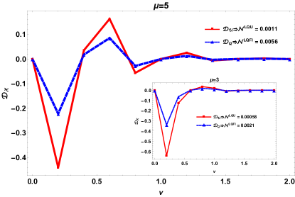
Figure 5: The time derivation $\mathcal{D}_{\mathcal{X}}\left(\mathcal{X}\equiv\mathcal{U,Q}\right)$ versus the dimensionless time $\nu$ for the parameter $\mu=3$ and $\mu=5$. The non-Markovian time periods are those where $D_{\mathcal{X}}>0$.

Here, we have done the same for a non-Markovian depolarization channel based on a different initial state 59. We obtained the results represented in Fig.5 which represents $\mathcal{D}_{\mathcal{X}}\left(\nu\right)>0\left(\mathcal{X}\equiv\mathcal{U,Q}\right)$ as function $\nu$ for different values of $\mu$. It is worth noting that an increase in the parameter $\mu$ corresponds to an increase in the degree of non-Markovianity, quantified by the measure $\mathcal{N}^{LQFI}$. Conversely, an increase in $\mu$ is associated with a decrease in the degree of non-Markovianity, measured by $\mathcal{N}^{LQU}$. Indeed, as previously the same remarks when $\mathcal{D}_{\mathcal{X}}\left(\nu\right)>0$ mean that the dynamics of the system are non-Markovian, and $\mathcal{D}_{\mathcal{X}}\left(\nu\right)<0$ the system is Markovian. Considering the results obtained here i.e. for a non-Markovian depolarization channel, they agree with the result obtained in the first and second sections for the phase damping channel and the amplitude damping channel means that always $\mathcal{N}^{LQFI}\geq\mathcal{N}^{LQU}$.

Hence, it is evident from the above examples that the structure of the reservoir influences the non-Markovian nature of the dynamics. In the phase damping dynamical model, non-Markovianity is observed in the super ohmic regime. For the amplitude damping channel, non-Markovianity is present within the small range $0.18\leq\lambda/\gamma_{0}\leq 0.43$. The dephasing model $\mathcal{N}^{LQFI}$ demonstrates an increasing trend with higher values of $\mu$, suggesting a growing degree of non-Markovianity. Conversely, $\mathcal{N}^{LQU}$ exhibits a decreasing trend with higher values of $\mu$, indicating a reduction in non-Markovian behavior. Indeed, all three examples support the inequality (22).

IV Concluding Remarks and Outlook

To conclude, we have developed a new metric for non-Markovianity from the perspective of non-classical correlations using local quantum Fisher information. This measure has been applied to three common noisy channels: the phase damping channel, the amplitude damping channel, and the depolarizing channel. We conducted a comparative analysis of the relationship between our proposed measure and another typical measure based on local quantum uncertainty LQU. It has been shown that for these three channels, the proposed measure is consistent with the LQU-based measure. However, there is a difference in the degree of non-Markovianity: the measure based on LQFI indicates a greater degree of non-Markovianity compared to the LQU-based measure. Most importantly, the current investigation suggests that LQFI-based and LQU-based measures of non-Markovianity exhibit similar variation patterns. This work highlights the relevance of these specific types of non-Markovianity measures.

In addition, it is important to highlight the relationships between our measure and other established measures of non-Markovianity, such as information backflow and divisibility. Despite the consistency in detecting non-Markovianity across different measures, our approach is conceptually distinct. For example, the information backflow measure is based on trace distance, while the divisibility measure relies on violations of the divisibility law and the Jamiolkowski-Choi isomorphism. Compared to the LQU-based non-Markovianity measure, our LQFI-based measure offers a unique perspective for capturing the information dynamics of open quantum systems. Our results indicate that a positive time derivative of LQFI signals the flow of information from the environment to the system, indicative of non-Markovian dynamics. This underscores the influence of reservoir structure on the Markovian/non-Markovian character of an open quantum system. We believe our measure provides a valuable tool for characterizing non-Markovianity, facilitating both theoretical descriptions and experimental investigations. As a truly quantitative measure, it assesses the degree of non-Markovianity across different physical systems and is computationally easier to evaluate compared to LQU-based measure. We expect that non-Markovianity based on LQFI will significantly contribute to further research in open quantum systems. The relationship between various non-Markovian quantifications remains a pertinent topic for future research, despite numerous discoveries in recent years.

References

- [1] J. P. Dowling, and G. J. Milburn, Quantum technology: the second quantum revolution, Phil. Trans. R. Soc. A, 361 (2003) 1655-1674.
- [2] T. D. Ladd, F. Jelezko, R. Laflamme, Y. Nakamura, C. Monroe, and J. L. O’Brien, Quantum computers, nature, 464 (2010) 45-53.
- [3] N. Ikken, A. Slaoui, R. Ahl Laamara and L. B. Drissi, Bidirectional quantum teleportation of even and odd coherent states through the multipartite Glauber coherent state: theory and implementation, Quantum Inf Process, 22 (2023) 391.
- [4] A. Slaoui, N. Ikken, L. B. Drissi, and R. A. Laamara, Quantum Communication Protocols: From Theory to Implementation in the Quantum Computer, (2023).
- [5] H. P. Breuer, and F.Petruccione, The theory of open quantum systems. Oxford University Press, USA (2002).
- [6] W. H. Zurek, Decoherence, einselection, and the quantum origins of the classical, Rev. Mod. Phys, 75 (2003) 715.
- [7] Y. Dakir, A. Slaoui, AB.A. Mohamed, R. Ahl Laamara and H. Eleuch, Quantum teleportation and dynamics of quantum coherence and metrological non-classical correlations for open two-qubit systems, Sci Rep, 13 (2023) 20526.
- [8] H. Carmichael, An open systems approach to quantum optics: lectures presented at the Université Libre de Bruxelles, October 28 to November 4, 1991 (Vol. 18), Springer Science & Business Media, (2009).
- [9] A. Slaoui, A. Salah, and M. Daoud, Influence of Stark-shift on quantum coherence and non-classical correlations for two two-level atoms interacting with a single-mode cavity field, Physica A, 558 (2020) 124946.
- [10] N-E. Abouelkhir, A. Slaoui, H. El Hadfi, and R. Ahl Laamara, Estimating phase parameters of a three-level system interacting with two classical monochromatic fields in simultaneous and individual metrological strategies, J. Opt. Soc. Am. B, 40 (2023) 1599-1610.
- [11] T. C. Ralph, Quantum optical systems for the implementation of quantum information processing, Rep. Prog. Phys, 69 (2006) 853.
- [12] V. Gorini, A. Kossakowski, and E. C. G. Sudarshan, Completely positive dynamical semigroups of N-level systems, J. Math. Phys, 17 (1976) 821-825.
- [13] G. Lindblad, On the generators of quantum dynamical semigroups, Commun. Math. Phys, 48 (1976) 119-130.
- [14] H. P. Breuer, E. M. Laine, and J. Piilo, Measure for the degree of non-Markovian behavior of quantum processes in open systems.Phys. Rev. Lett, 103 (2009) 210401.
- [15] A. Slaoui, M. Daoud, and R.A. Laamara, The dynamics of local quantum uncertainty and trace distance discord for two-qubit X states under decoherence: a comparative study, Quantum Inf Process, 17 (2018) 178.
- [16] E. M. Laine, J. Piilo, and H. P. Breuer, Measure for the non-Markovianity of quantum processes, Phys. Rev. A, 81 (2010) 062115.
- [17] S. C.Hou, X. X. Yi, S. X. Yu, C. H. Oh, Alternative non-Markovianity measure by divisibility of dynamical maps, Phys. Rev. A, 83 (2011) 062115.
- [18] S. F. Huelga, A. Rivas, and M. B. Plenio, Non-Markovianity-assisted steady state entanglement, Phys. Rev. Lett, 108 (2012) 160402.
- [19] E.-M. Laine, H.-P. Breuer, J. Piilo, C.-F. Li, and G.-C. Guo, Nonlocal memory effects in the dynamics of open quantum systems, Phys. Rev. Lett, 108 (2012) 210402.
- [20] A. W. Chin, S. F. Huelga, and M. B. Plenio, Quantum metrology in non-Markovian environments, Phys. Rev. Lett, 109 (2012) 233601.
- [21] Z.-Y. Xu, S. Luo, W. L. Yang, C. Liu, and S. Zhu, Quantum speedup in a memory environment, Phys. Rev. A, 89 (2014) 012307.
- [22] S. Deffner and E. Lutz, Quantum speed limit for non-Markovian dynamics, Phys. Rev. Lett, 111 (2013) 010402.
- [23] K. Siudzińska, Markovian semigroup from mixing noninvertible dynamical maps, Phys. Rev. A, 103 (2021) 022605.
- [24] M. M. Wolf, J. Eisert, T. S. Cubitt, and J. I. Cirac, Assessing non-Markovian quantum dynamics, Phys. Rev. Lett, 101 (2008) 150402.
- [25] S. Wißmann, H. P. Breuer, and B. Vacchini, Generalized trace-distance measure connecting quantum and classical non-Markovianity, Phys. Rev. A, 92 (2015) 042108.
- [26] F. Settimo, H. P. Breuer, and B. Vacchini, Entropic and trace-distance-based measures of non-Markovianity, Phys. Rev. A, 106 (2022) 042212.
- [27] A. K. Rajagopal, A. U. Devi, and R. W. Rendell, Kraus representation of quantum evolution and fidelity as manifestations of Markovian and non-Markovian forms, Phys. Rev. A, 82 (2010) 042107.
- [28] Á. Rivas, S. F. Huelga and M. B.Plenio, Entanglement and non-Markovianity of quantum evolutions, Phys. Rev. Lett, 105 (2010) 050403.
- [29] H. Yuen and M. Lax, Multiple-parameter quantum estimation and measurement of nonselfadjoint observables, IEEE Transactions on Information Theory, 19, (1973) 740-750.
- [30] X. M. Lu, X. Wang, and C. P. Sun, Quantum Fisher information flow and non-Markovian processes of open systems, Phys. Rev. A, 82 (2010) 042103.
- [31] H. Song, S. Luo, and Y. Hong, Quantum non-Markovianity based on the Fisher-information matrix, Phys. Rev. A, 91 (2015) 042110.
- [32] B. Bylichka, D. Chruściński and S. Maniscalco, Non-Markovianity and reservoir memory of quantum channels: a quantum information theory perspective, Sci Rep, 4 (2014) 5720.
- [33] S. Luo, S. Fu, H. Song, Quantifying non-Markovianity via correlations, Phys. Rev. A, 86 (2012) 044101.
- [34] Z. He, H. S. Zeng, Y. Li, Q. Wang and C. Yao, Non-Markovianity measure based on the relative entropy of coherence in an extended space, Phys. Rev. A, 96 (2017) 022106.
- [35] Z. He, C. Yao, Q. Wang, J. Zou, Measuring non-Markovianity based on local quantum uncertainty, Phys. Rev. A, 90 (2014) 042101.
- [36] P. Haikka, J. D.Cresser, and S.Maniscalco, Comparing different non-Markovianity measures in a driven qubit system, Phys. Rev. A, 83 (2011) 012112.
- [37] D. Girolami, T. Tufarelli, and G. Adesso, Characterizing nonclassical correlations via local quantum uncertainty, Phys. Rev. Lett, 110 (2013) 240402.
- [38] E. P.Wigner, and M. M.Yanase, Information contents of distributions, Proceedings of the National Academy of Sciences, 49 (1963) 910-918.
- [39] S. Kim, L. Li, A. Kumar, and J. Wu, Characterizing nonclassical correlations via local quantum Fisher information, Phys. Rev. A, 97 (2018) 032326.
- [40] G. Tóth and I. Apellaniz, Quantum metrology from a quantum information science perspective, J. Phys. A: Math. Theor, 47 (2014) 424006.
- [41] A. Slaoui, L. Bakmou, M. Daoud, and R. A. Laamara, A comparative study of local quantum Fisher information and local quantum uncertainty in Heisenberg XY model, Phys. Lett. A, 383 (2019) 2241-2247.
- [42] A. Jamiołkowski, Linear transformations which preserve trace and positive semidefiniteness of operators. Rep. Math. Phys, 3 (1972) 275-278.
- [43] P. Haikka, T. H. Johnson, and S. Maniscalco, Non-Markovianity of local dephasing channels and time-invariant discord, Phys. Rev. A, 87 (2013) 010103.
- [44] Z. He, J. Zou, L. Li, and B. Shao, Effective method of calculating the non-Markovianity N for single-channel open systems, Phys. Rev. A, 83 (2011) 012108.
- [45] S. Maniscalco, F. Petruccione, Non-Markovian dynamics of a qubit, Phys. Rev. A, 73 (2006) 012111.
- [46] S. Daffer, K. Wodkiewicz, J. D. Cresser, and J. K. Mclver, Phys. Rev. A, 70 (2004) 010304.
- [47] K. Kraus, A. Böhm, J. D. Dollard, and W. H.Wootters, (Eds.), States, Effects, and Operations Fundamental Notions of Quantum Theory: Lectures in Mathematical Physics at the University of Texas at Austin. Berlin, Heidelberg: Springer Berlin Heidelberg (1983).