Aggregation-diffusion in heterogeneous environments

Abstract

Aggregation-diffusion equations are foundational tools for modelling biological aggregations. Their principal use is to link the collective movement mechanisms of organisms to their emergent space use patterns in a rigorous, non-speculative way. However, most existing studies implicitly assume that organism movement is not affected by the underlying environment. In reality, the environment is a key determinant of emergent space use patterns, albeit in combination with collective aspects of motion. This work studies aggregation-diffusion equations in a heterogeneous environment in one spatial dimension. Under certain assumptions, it is possible to find exact analytic expressions for the steady-state solutions to the equation when diffusion is quadratic. Minimising the associated energy functional across these solutions provides a rapid way of determining the likely emergent space use pattern, which can be verified via numerics. This energy-minimisation procedure is applied to a simple test case, where the environment consists of a single clump of attractive resources. Here, self-attraction and resource-attraction combine to shape the emergent aggregation. Two counter-intuitive results emerge from the analytic results: (a) a non-monotonic dependence of clump width on the aggregation width, (b) a positive correlation between self-attraction strength and aggregation width when the resource attraction is strong. These are verified through numerical simulations. Overall, the study shows rigorously how environment and collective behaviour combine to shape organism space use, sometimes in counter-intuitive ways.

MSC Classification]35B36, 35B38, 35Q92, 92C15, 92C17, 92D40

1 Introduction

Aggregation phenomena are widespread in the natural world, from swarming [35], flocking [29], and herding [37] of animals to cellular aggregations in embryonic patterns [42] and slime mould slugs [6]. This has led to a proliferation of research into the possible mechanisms that could cause these aggregations to form [27]. A popular mathematical tool for analysing this problem is the aggregation-diffusion equation [12]. This is a partial differential equation (PDE) model that assumes organisms have two aspects to their movement. One is an attraction to other nearby organisms of the same kind, often called self-attraction (where ‘self’ refers here to the population rather than the individual), which is encoded in a non-local advection term. The other is a diffusive aspect to their movement, which is a simple catch-all for all the aspects of movement that are not explicitly related to aggregation, for example foraging or exploring.

Although models of diffusion and non-local advection have been instrumental in understanding the mechanisms of biological aggregation and related phenomena, they are typically analysed in a homogeneous environment [27, 41]. This implicitly assumes that the environment in which the organisms live has negligible effect on the aggregation. However, it is well-known that, in many biological situations, there are environmental drivers factors that work alongside self-attraction to drive the emergent spatial patterns of organisms [5, 23, 26, 38].

For example, in the embryonic development of hair and feather follicles, cells form aggregates that are driven at least in part by movement up the gradient of a chemical attractant from a point source. They may also have self-aggregation properties to their movement. Currently, it is often not clear which is the principal driver of this movement, or whether both aspects work in combination [13, 21]. In animal ecology, space use patterns are governed in part by proximity to resources that are fundamental for survival (e.g. food, water, shelter) [1, 9, 40]. Yet many species are highly social and show attraction towards conspecifics, as well as being attracted to familiar areas (a phenomenon called ‘home ranging’, that can be viewed as a form of aggregation [10, 8]). Therefore, like the cellular case, the space use patterns of animals emerge from a combination of self-attraction and attraction to environmental resources [22, 14, 31].

Here, as a first step towards understanding how the environment and self-attraction might combine to shape aggregative patterns, we study the aggregation-diffusion equation in a static heterogeneous environment in one spatial dimension. It is possible to gain analytic insight into the steady state solutions under certain conditions. Specifically, we first assume diffusion is quadratic and that the environment can be decomposed as a Fourier series. Then we either assume that the non-local advection has a particular functional form that allows for exact analysis (namely the Laplace kernel) or approximate the system via a Taylor expansion closed at the second moment. These two models are detailed in Section 2. With these conditions in place, the steady state solutions to the system are fully classified in Section 3.

Next, to understand which of the steady state solutions are likely to be observed in reality (i.e. in numerical experiments), we examine the energy functional associated to the system and minimise it across the possible steady states. In Section 4 we perform this minimisation procedure for a particular functional form of the environment, related to a single clump of attractive resources. In the case of cells, this could be thought of as a chemical gradient arising from a point source. For animals, this models an area of high forage in amongst low-forage surroundings. The energy minimisation procedure turns out to be very rapid, as it only involves searching through a single variable across a finite range of values. This enables us to ascertain quickly how the functional form of the minimum energy steady state solution varies with the model parameters, without the need for time-consuming numerical PDEs.

In Section 5, we explore numerically the extent to which the lessons from our analytic study extend to situations that are not amenable to mathematical analysis. Specifically, we focus on different functional forms for the non-local kernel and linear diffusion alongside quadratic. Linear diffusion, whilst not so mathematically amenable as quadratic diffusion (at least in our case), is perhaps more natural biologically. So it is interesting to see whether our analytic results carry over to different situations that may be slightly closer to the underlying biological reality.

2 The model

Let $u(x,t)$ denote the population density across space, $x$, of a group of organisms at time $t$. The population is assumed to be of fixed size, so that any pattern formation is governed purely by the organisms’ movement. The organisms each have a diffusive aspect to their movement, as well as non-local attraction to other organisms, and a tendency to move up the gradient of a fixed environment, given by $A(x)$. In one spatial dimension, this leads to the following model

$$\frac{\partial u}{\partial t} =\frac{D}{k}\frac{\partial^{2}}{\partial x^{2}}(u^{k})-\frac{\partial}{\partial x}\left[u\left(\gamma\frac{\partial}{\partial x}(K\ast u)+\frac{\partial A}{\partial x}\right)\right],$$ (1)

where $D,\gamma>0$ are positive real constants, $k>0$ is a constant integer, $K(x)$ is a symmetric probability density function (so integrates to 1 over the domain of definition) with finite variance, and

$$K\ast u(x)=\int_{-\infty}^{\infty}K(z)u(x+z){\rm d}z$$ (2)

is a convolution. Equation (1) is an aggregation-diffusion equation [12], with an additional term denoting flow up the gradient of the environment, $A(x)$.

For most of this manuscript, in particular for deriving all the analytic results, we will be focusing on the quadratic diffusion case, $m=2$, which rearranges to the following form

$$\frac{\partial u}{\partial t} =\frac{\partial}{\partial x}\left[u\left(D\frac{\partial u}{\partial x}-\gamma\frac{\partial}{\partial x}(K\ast u)-\frac{\partial A}{\partial x}\right)\right].$$ (3)

The non-local term, $K\ast u$, in Equation (3) makes analytic studies tricky in general. However, there are two things we can do to ease matters. First, it turns out that the Laplace kernel has some nice properties that allow for exact analysis. We will denote the Laplace kernel by $K_{m}(x)=m{\rm e}^{-m|x|}/2$ to separate it from the general kernel, $K$.

Second, for any $K$ that is symmetric and has finite variance, we can make the following second order approximation

$$K\ast u\approx u+\frac{\sigma^{2}}{2}\frac{\partial^{2}u}{\partial x^{2}},$$ (4)

where $\sigma$ is the variance of $K$ (note that symmetry of $K$ means it has zero mean). This approximation enables us to replace Equation (3) with the following local fourth-order equation

$$\frac{\partial u}{\partial t} =\frac{\partial}{\partial x}\left[u\left(D\frac{\partial u}{\partial x}-\gamma\frac{\partial u}{\partial x}-\frac{\gamma\sigma^{2}}{2}\frac{\partial^{3}u}{\partial x^{3}}-\frac{\partial A}{\partial x}\right)\right].$$ (5)

Most results in the manuscript will be expressed for either Equation (3) with $K=K_{m}$ or Equation (5) or both.

Subsequent analysis will focus on functional forms for $A(x)$ that are periodic on the interval $[-L,L]$ (i.e. $A(qL)=A(qL-2L)$ for all $q\in{\mathbb{Z}}$) so can be decomposed as the following Fourier series

$$A(x)=a_{0}+\sum_{n=1}^{\infty}\left[a_{n}\cos\left(\frac{n\pi x}{L}\right)+b_{n}\sin\left(\frac{n\pi x}{L}\right)\right].$$ (6)

To ease analysis, we will use the following non-dimensionalisation

$$\tilde{x}=\frac{x}{L},\,\tilde{\sigma}=\frac{\sigma}{L},\,\tilde{\gamma}=\frac{\gamma}{D},\,\tilde{A}(\tilde{x})=\frac{L}{D}A(x),\,\tilde{t}=\frac{tD}{L^{3}},\,\tilde{u}=Lu,\,\tilde{a}_{n}=\frac{La_{n}}{D},\,\tilde{b}_{n}=\frac{Lb_{n}}{D}.$$ (7)

Immediately dropping the tildes for notational convenience leads to the following dimensionless versions of Equation (3), written here with $K=K_{m}$

$$\frac{\partial u}{\partial t} =\frac{\partial}{\partial x}\left[u\left(\frac{\partial u}{\partial x}-\gamma\frac{\partial}{\partial x}(K_{m}\ast u)-\frac{\partial A}{\partial x}\right)\right],$$ (8)

and the following dimensionless version of Equation (5)

$$\frac{\partial u}{\partial t} =\frac{\partial}{\partial x}\left(u\frac{\partial}{\partial x}\left[(1-\gamma)u-\frac{\gamma\sigma^{2}}{2}\frac{\partial^{2}u}{\partial x^{2}}-A\right]\right),$$ (9)

where

$$A(x)=a_{0}+\sum_{n=1}^{\infty}\left[a_{n}\cos\left({n\pi x}\right)+b_{n}\sin\left({n\pi x}\right)\right].$$ (10)

Equations (8) and (9) will be the main study equations for Sections 3 and 4.

3 Steady states and energy minimisers

Here, we classify all the steady state solution to Equations (8) and (9). The results are summarised in two propositions.

Proposition 1.

Suppose $u_{\ast}(x)$ is a steady state solution to Equation (8), with $A(x)$ as given in Equation (10). Suppose the support of $u_{\ast}(x)$ is bounded. On any connected component of the support of $u_{\ast}(x)$, the following holds

$$u_{\ast}(x)=u_{P}(x)+u_{I}(x)$$ (11)

where

$$u_{P}(x) =\alpha_{0}+\sum_{n=1}^{\infty}\frac{n^{2}\pi^{2}+m^{2}}{n^{2}\pi^{2}+m^{2}(1-\gamma)}\left[a_{n}\cos\left(n\pi x\right)+b_{n}\sin\left(n\pi x\right)\right],$$ (12)

$$u_{I}(x) =\begin{cases}P\sin\left(x\sqrt{m^{2}(\gamma-1)}\right)+Q\cos\left(x\sqrt{m^{2}(\gamma-1)}\right),&\mbox{if $\gamma>1$},\\ P\exp\left(x\sqrt{m^{2}(1-\gamma)}\right)+Q\exp\left(-x\sqrt{m^{2}(1-\gamma)}\right),&\mbox{if $\gamma<1$},\end{cases}$$ (13)

and $P,Q,\alpha_{0}\in{\mathbb{R}}$ are arbitrary constants.

Proof. Steady states of Equation (3), denoted $u_{\ast}(x)$, satisfy

$$C =u_{\ast}\left(\frac{{\rm d}u_{\ast}}{{\rm d}x}-\gamma\frac{\rm d}{{\rm d}x}(K_{m}\ast u_{\ast})-\frac{{\rm d}A}{{\rm d}x}\right),$$ (14)

for some constant $C$. As the support of $u_{\ast}(x)$ is bounded, the flux is zero sufficiently far from the origin, so $C=0$. Hence

$$0 =u_{\ast}\frac{{\rm d}}{{\rm d}x}\left(u_{\ast}-\gamma K_{m}\ast u_{\ast}-A\right).$$ (15)

Then, on any connected component of the support of $u_{\ast}(x)$ (i.e. where $u_{\ast}(x)\neq 0$), we have

$$c+A =u_{\ast}-\gamma K_{m}\ast u_{\ast},$$ (16)

for some constant $c$. Now we apply a particular property of the Laplace kernel, namely that it satisfies

$$\frac{{\rm d}^{2}K_{m}}{{\rm d}x^{2}}-m^{2}K_{m}+m^{2}\delta(x)=0,$$ (17)

where $\delta(x)$ is the Dirac delta function. Applying the operator $m^{2}-\frac{\partial^{2}}{\partial x^{2}}$ to Equation (16) gives

$$m^{2}c+m^{2}A(x)-\frac{{\rm d}^{2}A}{{\rm d}x^{2}} =m^{2}(1-\gamma)u_{*}-\frac{{\rm d}^{2}u_{*}}{{\rm d}x^{2}},$$ (18)

which is an inhomogeneous second order ODE with constant coefficients. A direct calculation shows that Equation (18) is solved by Equations (11)-(13) by setting $\alpha_{0}=(c+a_{0})/(1-\gamma)$. ∎

Proposition 2.

Suppose $u_{\ast}(x)$ is a steady state solution to Equation (9), with $A(x)$ as given in Equation (10). Suppose the support of $u_{\ast}(x)$ is bounded. On any connected component of the support of $u_{\ast}(x)$, the following holds

$$u_{\ast}(x)=u_{P}(x)+u_{I}(x)$$ (19)

where

$$u_{P}(x) =\alpha_{0}+\sum_{n=1}^{\infty}\frac{2}{2(1-\gamma)+\gamma\sigma^{2}n^{2}\pi^{2}}\left[\alpha_{n}\cos\left(n\pi x\right)+\beta_{n}\sin\left(n\pi x\right)\right],$$ (20)

$$u_{I}(x) =\begin{cases}P\sin\left(x\sqrt{\frac{2(\gamma-1)}{\gamma\sigma^{2}}}\right)+Q\cos\left(x\sqrt{\frac{2(\gamma-1)}{\gamma\sigma^{2}}}\right),&\mbox{if $\gamma>1$},\\ P\exp\left(x\sqrt{\frac{2(1-\gamma)}{\gamma\sigma^{2}}}\right)+Q\exp\left(-x\sqrt{\frac{2(1-\gamma)}{\gamma\sigma^{2}}}\right),&\mbox{if $\gamma<1$},\end{cases}$$ (21)

and $P,Q,\alpha_{0}\in{\mathbb{R}}$ are arbitrary constants.

Proof. Any steady state, $u(x,t)=u_{\ast}(x)$, of Equation (9) satisfies

$$C =u_{\ast}\left(\frac{{\rm d}u_{\ast}}{{\rm d}x}-\gamma\frac{{\rm d}u_{\ast}}{{\rm d}x}-\frac{\gamma\sigma^{2}}{2}\frac{{\rm d}^{3}u_{\ast}}{{\rm d}x^{3}}-\frac{{\rm d}A}{{\rm d}x}\right),$$ (22)

for some constant $C$. Since the support of $u_{\ast}(x)$ is bounded, the flux is zero sufficiently far from the origin, so $C=0$. Therefore, as in the proof of Proposition 1, on any connected component of the support of $u_{\ast}$, we have

$$c+A=(1-\gamma)u_{\ast}-\frac{\gamma\sigma^{2}}{2}\frac{{\rm d}^{2}u_{\ast}}{{\rm d}x^{2}},$$ (23)

for some constant $c$. A direct calculation shows that Equation (23) is solved by Equations (19)-(21) by setting $\alpha_{0}=(c-a_{0})/(\gamma-1)$. ∎

Whilst these two propositions fully-categorise all possible steady state solutions, $u_{\ast}(x)$, the story is not finished. First, there are three unknowns that the results introduce: $\alpha_{0}$, $P$, $Q$. Furthermore, the expressions in Equations (11)-(13) and (19)-(21) are only valid on connected components of the support of $u_{\ast}(x)$. This leaves open the question as to which of the various possible steady states the PDE system might actually tend towards, given an initial condition.

To gain insight into this, we look for solutions that minimise the associated energy functional [17]. For Equation (8), this functional is

$$E_{1}[u]=\int_{\infty}^{\infty}u\left[(1-\gamma)u-2A-\gamma K_{m}*u\right]{\rm d}x.$$ (24)

A direct calculation shows that

$$\frac{{\rm d}E_{1}}{{\rm d}t}=-\int_{\Omega}2u\left(\frac{\partial}{\partial x}\left[u-A-\gamma K_{m}*u\right]\right)^{2}{\rm d}x,$$ (25)

as long as $u(x)$ vanishes for all $x$ arbitrarily far from the origin. This means that $E_{1}[u]$ is non-increasing in time as long as $u$ remains non-negative, and is zero when Equation (8) is at steady state.

The energy for Equation (9) is

$$E_{2}[u]=\int_{\infty}^{\infty}u\left[(1-\gamma)u-2A-\frac{\gamma\sigma^{2}}{2}\frac{\partial^{2}u}{\partial x^{2}}\right]{\rm d}x.$$ (26)

Similarly, a direct calculation shows that

$$\frac{{\rm d}E_{2}}{{\rm d}t}=-\int_{\Omega}2u\left(\frac{\partial}{\partial x}\left[(1-\gamma)u-A-\frac{\gamma\sigma^{2}}{2}\frac{\partial^{2}u}{\partial x^{2}}\right]\right)^{2}{\rm d}x,$$ (27)

as long as $u(x)$ vanishes for all $x$ arbitrarily far from the origin. Therefore, as before, $E_{2}[u]$ is non-increasing in time as long as $u$ remains non-negative, and is zero when Equation (9) is at steady state.

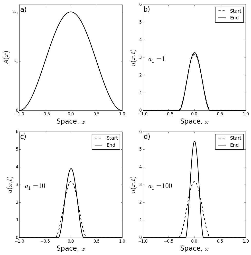
Figure 1: Aggregation in a single-clumped landscape: numerics. Panel (a) shows $A(x)=a_{1}\cos(\pi x)$, a single clump of attractive resources centred on $x=0$. With this functional form of $A(x)$ in place, Panels (b)-(d) show initial and final numerical solutions for Equation (5), for example values of $a_{1}$.

4 Landscapes with a single clump of attractive resources

As mentioned in the Introduction, we focus our attention on a particular case of biological interest: where the landscape $A(x)$ consists of a single clump of attractive material. The aim is to disentangle the landscape and self-attractive effects on the size and shape of the resulting aggregation. The functional form for $A(x)$ we use to model this situation is as follows

$$A(x)=\begin{cases}a_{n}[1+\cos(n\pi x)],&\mbox{if $|x|<\frac{1}{n}$,}\\ 0,&\mbox{otherwise.}\end{cases}$$ (28)

Our analysis will focus on the fourth-order model of Equation (9). Calculations for the Laplace model of Equation (8) are rather similar, so we report these in Appendix A.

In numerical experiments, if we start with aggregated initial conditions, we remain in an aggregation, albeit one of a different size. This is shown in Figure 1, which uses initial conditions from a steady-state minimum-energy solution to Equation (9) with $a_{n}=0$, $\gamma=2$, $\sigma=0.1$, and total population size $p=1$. This solution has the following form (first shown in Falcó et al [15, Section 2.3.1], but also reported in Appendix B with a slightly different proof)

$$u_{\ast}(x)=\begin{cases}\frac{p}{2r_{0}}\left[1+\cos\left(\frac{x\pi}{r_{0}}\right)\right],&\mbox{if $-r_{0}<x<r_{0}$,}\\ 0,&\mbox{otherwise,}\end{cases}$$ (29)

where

$$r_{0}=\pi\sqrt{\frac{\gamma\sigma^{2}}{2(\gamma-1)}}.$$ (30)

Note that $p$ is constant over time and can be calculated as

$$p=\int_{-\infty}^{\infty}u(x,t){\rm d}x.$$ (31)

From the initial condition of Equation (29), Figure 1 shows steady-state numerical solutions of Equation (9), calculated using the algorithm from Falcó et al [15], keeping $\gamma=2$ and $\sigma=0.2$ fixed but using different values of $a_{1}$. Each steady state was estimated by running the algorithm until $|u(x,t)-u(x,t+\Delta t)|<10^{-8}$ for all $x$, where $\Delta t=10^{-7}$.

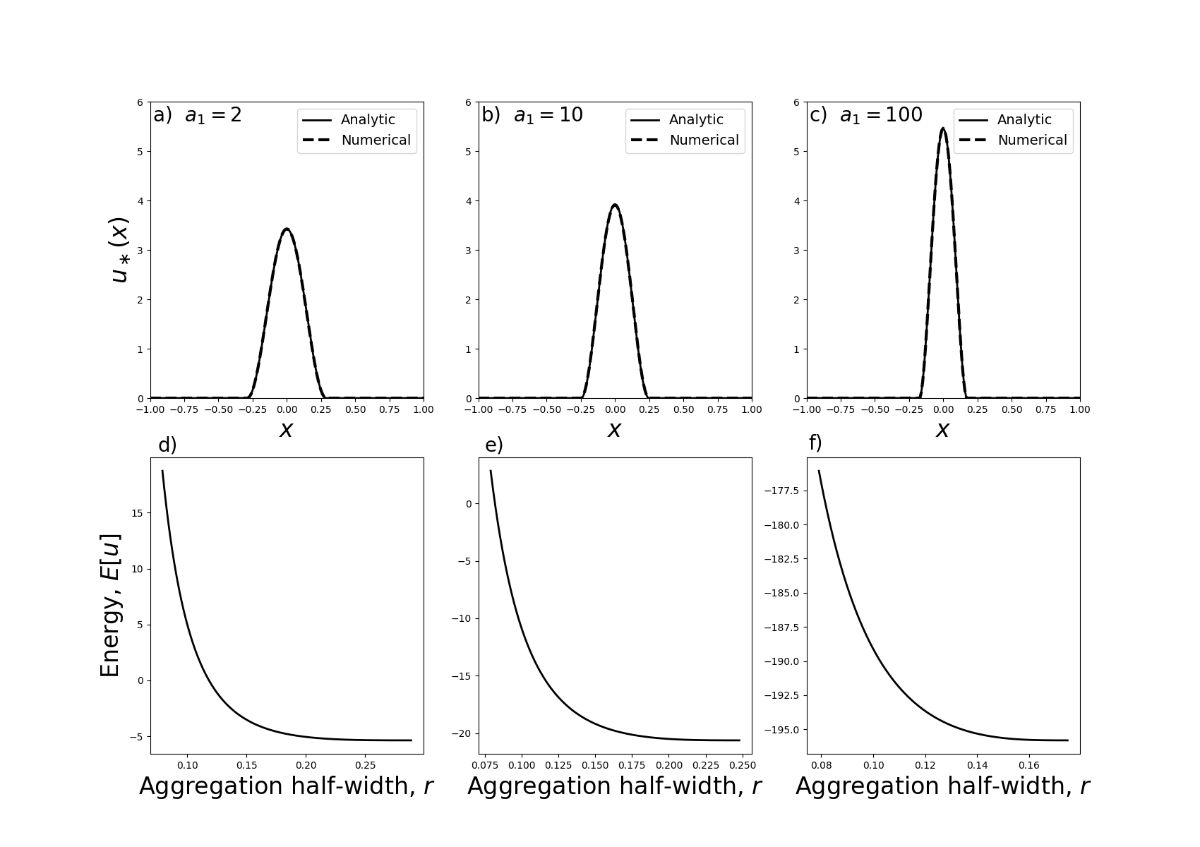
Figure 2: Aggregation in a single-clump landscape: minimum energy solutions. Panels (a), (b), and (c) show the minimum energy solution of the form given by Equations (32)-(34) (solid curves), for $n=1$, alongside the numerical steady-state solution (dashed curves) for different values of $a_{1}$ given in the plots. Panels (d), (e), and (f) show the energy as a function of $r$ for the values of $a_{1}$ given in Panels (a), (b), and (c) respectively. The respective minimum energy $r$-values are $r=0.289,r=0.248,$ and $r=0.175$.

Each numerical steady-state solution appears to be supported on a single interval $[-r,r]$, symmetric about zero. We therefore restrict our search for minimum energy solutions, from the possible solutions found in Section 3, to this type of symmetric, single-aggregation solution. In the fourth-order model of Equation (9), such solutions have the following form (derived from Equations (19)-(21) and (28)),

$$u_{\ast}(x)=\begin{cases}\alpha_{0}+\alpha_{n}[1+\cos(\pi nx)]+Q\cos\left(\frac{x\pi}{r_{0}}\right),&\mbox{for $x\in\left[-\frac{1}{n},\frac{1}{n}\right]\cap[-r,r]$,}\\ \alpha_{0}+Q\cos\left(\frac{x\pi}{r_{0}}\right),&\mbox{for $\frac{1}{n}<|x|\leq r$ if $r>\frac{1}{n}$,}\\ 0,&\mbox{otherwise,}\end{cases}$$ (32)

where $0<r\leq 1$. Applying the integral condition from Equation (31) gives

$$\alpha_{0}=\begin{cases}\frac{p}{2r}-\alpha_{n}-\frac{\alpha_{n}}{\pi nr}\sin(\pi nr)-\frac{Qr_{0}}{\pi r}\sin\left(\frac{r\pi}{r_{0}}\right),&\mbox{if $r<1/n$,}\\ \frac{p}{2r}-\frac{\alpha_{n}}{nr}-\frac{Qr_{0}}{\pi r}\sin\left(\frac{r\pi}{r_{0}}\right),&\mbox{otherwise,}\end{cases}$$ (33)

so that the two remaining free parameters are $r$ and $Q$. We restrict our search further by only looking for continuous solutions.

Figure 3: Dependence of aggregation size on model parameters. Aggregation sizes refer to minimum energy steady-state solutions to Equation (9) with $A(x)$ as given in Equation (28), and calculated using the procedure from Section 4. Unless otherwise stated, $n=1$, $a_{n}=1$, $\gamma=2$, and $\sigma=0.1$.

This gives the additional constraint

$$Q=\begin{cases}-\frac{\alpha_{0}+\alpha_{n}+\alpha_{n}\cos(\pi nr)}{\cos(r\pi/r_{0})},&\mbox{if $r<1/n$,}\\ -\frac{\alpha_{0}}{\cos(r\pi/r_{0})},&\mbox{otherwise.}\end{cases}$$ (34)

Plugging the expression for $u=u_{\ast}$ from Equation (32) into Equation (26) shows, after a direct calculation, that the energy functional we wish to minimise has the form

$$E_{2}[u_{\ast}]=\begin{cases}\int_{-r}^{r}u_{\ast}[(1-\gamma)(\alpha_{0}+\alpha_{n})-2a_{n}-a_{n}\cos(n\pi x)]{\rm d}x,&\mbox{if $r<1/n$,}\\ \int_{-1/n}^{1/n}u_{\ast}[(1-\gamma)(\alpha_{0}+\alpha_{n})-2a_{n}-a_{n}\cos(n\pi x)]{\rm d}x\\ \qquad+2\int_{1/n}^{r}u_{\ast}(1-\gamma)\alpha_{0}{\rm d}x,&\mbox{otherwise.}\end{cases}$$ (35)

Minimising Equation (35) requires a numerical search through the single remaining parameter, $r$. This can be done in a fraction of a second on an ordinary laptop (e.g. one with an Intel i7 2.8GHz processor), contrasting with numerical solutions to the underlying PDE, which typically take many minutes or even hours. Furthermore, once $r$ is found numerically, the minimum energy solution can be written down in an analytic form, namely that of Equations (32).

Figure 2 shows a few examples of such analytic solutions, together with their numerical counterparts, solved using the algorithm of Bailo et al [3] and Falcó et al [15]. Note that for certain values of $r\in(0,r_{0})$, the solution given by Equations (32)-(34) is not positive, so not allowable (see the positivity results of Bailo et al [2], Bailo et al [3]). Therefore the horizontal axes in Figures 2(d-f) do not go all the way from 0 to $r_{0}$.

Figure 4: Numerical verification of analytic insights. Panel (a) shows a zoomed-in version of the case $\sigma=0.1$ from Figure 3e. Panel (b) shows numerical steady state-solutions to Equation (9) corresponding to the parameters from Panel (a) (namely, $\gamma=2$, $a_{n}=1$, $\sigma=0.1$). Panel (c) shows the case $a_{1}=1000$ from Figure 3f and Panel (d) gives the corresponding numerical steady-state solutions.

This energy minimisation procedure enables rapid calculating of trends in the size of the aggregation as a function of the underlying parameters, without needing to perform time-consuming numerical PDEs. Figure 3 shows how the width of the minimum-energy aggregation of $u$, given by $2r$, depends upon both the width of the landscape’s peak, given by $2/n$, as well as the parameters $a_{n}$, $p$, $\gamma$, and $\sigma$. Interestingly, there is a non-monotonic dependence of the aggregation width of $u$ on width of the underlying landscape’s peak. This arises from analysing minimum energy solutions, but is also verified through numerical simulations. In Figure 4b, we see that the narrowest aggregation (and also highest peak) occurs for the intermediate value $n=6$. If resources are more clumped than this, i.e. if $n>6$, then rather than this causing the aggregations to be thinner, as might be expected, they are actually slightly wider.

Another counter-intuitive result occurs when we have a strong attraction to resources, e.g. $a_{n}=100$ or $a_{n}=1000$. Here, increasing $\gamma$ leads to a widening of the aggregation, contrary to what usually happens with no resources or a smaller resource attraction (Figure 3f). Again, this result plays out in the numerics (Figure 4d).

5 Numerical investigation

All the analytic results in Sections 3 and 4 rely on two features chosen purely for mathematical convenience: quadratic diffusion ($m=2$ in Equation 1) and either a fourth-order approximation to the non-local term or a Laplace kernel. These choices enable us to derive linear ODEs for the steady state that can be solved exactly. However, in many biological applications, linear diffusion is more natural than quadratic diffusion. For example, linear diffusion appears as the continuum limit of many random walk models used for organism movement [20, 30, 32, 34, 39]. Likewise, the Laplace kernel may not always be the most favourable choice from a biological modelling perspective [27]. Therefore it is worth investigating whether the analytic insights provided so far might carry over to other situations, including linear diffusion and different non-local kernels.

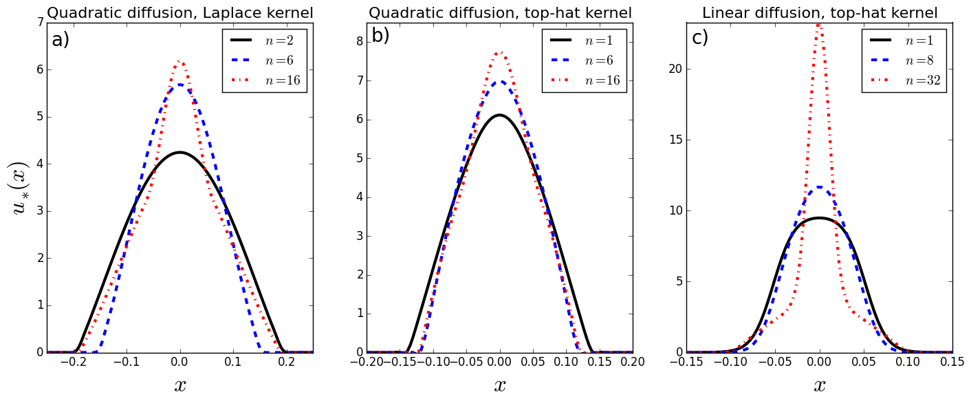
Figure 5: Numerical investigation. Panel (a) shows numerical steady state solutions of Equation (3) with a Laplace kernel (Equation 17), for various $n$ and $m=10$. Panel (b) shows numerical steady state solutions of Equation (3) with a top hat kernel (Equation 39), for various $n$ and $\delta=0.1$. Panel (c) shows numerical steady state solutions of Equation (36) with a top hat kernel with $\delta=0.1$. In all panels, $\gamma=2$, $a_{n}=1$, $p=1$, and $A(x)$ is as in Equation (28).

The linear diffusion model is given by $k=1$ in Equation (1). After applying the non-dimensionalisation from Equation (7) and dropping the tildes, this becomes

$$\frac{\partial u}{\partial t} =\frac{\partial^{2}u}{\partial x^{2}}-\frac{\partial}{\partial x}\left[u\left(\gamma\frac{\partial}{\partial x}(K\ast u)+\frac{\partial A}{\partial x}\right)\right].$$ (36)

To understand why numerical analysis is required in this case, we can follow the same argument as we did for quadratic diffusion to examine the steady state solutions of Equation (36). Any steady state, $u_{\ast}(x)$, satisfies the following

$$0 =\frac{{\rm d}}{{\rm d}x}\left[u_{\ast}\frac{{\rm d}}{{\rm d}x}\left(\ln(u_{\ast})-\gamma K\ast u_{\ast}-A\right)\right].$$ (37)

Then, using a similar argument to that given from Equations (14) to (16), we arrive at the following expression, valid on any connected component of the support of $u_{\ast}(x)$

$$c+A =\ln(u_{\ast})-\gamma K\ast u_{\ast}.$$ (38)

The $\ln(u_{\ast})$ term makes this non-linear, obviating exact mathematical analysis. Indeed, even if we use a fourth order expansion (or a Laplace kernel) to deal with the non-local term, $K\ast u_{\ast}$, exact solutions are not generally possible.

However, we can use the results from the quadratic diffusion case to guide numerical analysis of the linear diffusion model. In particular, it is interesting to examine whether the non-monotonic dependence or aggregation width, $r$, on resource-clump width, $2/n$, holds in the case of linear diffusion. Numerical steady-state solutions were examined for both the linear diffusion case (Equation 37) and quadratic diffusion (Equation 8) for two different kernels cases: where $K=K_{m}$, the Laplace distribution, and where $K={\mathcal{K}}_{\delta}$, the top-hat distribution given by

$${\mathcal{K}}_{\delta}(x)=\begin{cases}\frac{1}{2\delta},&\mbox{if $|x|<\delta$}\\ 0,&\mbox{otherwise.}\end{cases}$$ (39)

The top-hat distribution is chosen due to its popularity in biological modelling [27, 41].

Results are shown in Figure 5 for three of the four cases. The linear diffusion case with a Laplace kernel is omitted, since we did not see any evidence of the non-monotonic dependence of the resource clump width on the aggregation width in this case. However, we do see this phenomenon in the other three cases. When there is quadratic diffusion and a Laplace kernel (Figure 5a), the $n=2$ and $n=16$ cases have very similar widths towards the bottom of the aggregation, with $n=6$ markedly thinner. However, contrary to the steady states of the fourth-order local PDE shown in Figure 4b, the height of the $n=16$ case is higher than the $n=6$ case. Indeed, we see a notable thinning of the $n=16$ aggregation about about $u_{\ast}(x)=2.7$. A possible interpretation of this is that towards the bottom of the aggregation, the non-local self-attraction is dominating to push the aggregation towards the width it would be were there no resources, i.e. Equation (29). Yet in the very centre the aggregation, the thin resource clump dominates, and we see a change in shape.

This phenomenon is also present in Figure 5b, and is even more pronounced in Figure 5c, where the highest value of $n$ shown is $n=32$. In this case, whilst the aggregation is thicker than the $n=1$ or $n=8$ cases at the bottom, it is quite a bit thinner towards the top, and also much higher. Although we do not have analytic expressions for the plots in Figure 5, they do look reminiscent of the functional form in Equation (32): a weighted sum of two cosine functions with different widths (truncated when they reach their first minima before and after $0$).

Numerical solutions of Equations (36) were computed using a forward difference algorithm by discretising space into a lattice with spacing $\Delta x=0.01$ and time into intervals of length $\Delta t=10^{-5}$. Numerical solutions of Equations (3) used the algorithm of Bailo et al [3] with $\Delta x=0.01$ and $\Delta t=5\times 10^{-6}$. To estimate the steady state, each simulation was run until $|u(x,t)-u(x,t+\Delta t)|<10^{-8}$ for all $x$. Code for performing numerics is available on GitHub at https://github.com/jonathan-potts/AggDiffHet.

6 Discussion

This study analysed a PDE model of biological aggregation in heterogeneous environments, consisting of diffusion, non-local self-attraction (at the population level), and flow up the environmental gradient. These aspects of organisms movement combine to shape emergent space use patterns, which are characterised as minimum energy solutions to the model. In the case where diffusion is quadratic and the non-local self-attraction is either through a Laplace kernel or a fourth-order approximation, analytic expressions are derived for the steady states of the model. When the environment consists of a single clump of attractive resources, finding the minimum energy steady state solution is quick and simple, compared to solving the PDE numerically. This enables some counter-intuitive results to be uncovered about how the environment interplays with self attraction: (a) a non-monotonic dependence of resource clump width on the organisms’ aggregation width, and (b) a tendency for increased self-attraction to cause the emergent aggregation to increase in width, in situations where the resource attraction is very strong.

When making simplifications for the sake of analytic tractability, there is always a danger that the observed phenomena are just a feature of the simplified model and do not carry over to other, perhaps more realistic, modelling scenarios. Therefore our analysis is bolstered with numerical solutions of slightly-modified forms of our study PDE, focusing on the non-monotonic dependence mentioned in (a) above. This non-monotonic phenomenon seems to hold both when we examined a top-hat kernel rather than a fourth order approximation, and when we switched from quadratic to linear diffusion. Consequently, it seems that this phenomenon it is likely to be a genuine feature of biological aggregations and not just a quirk of a particular model formulation.

It is therefore worth making some conjectures about how this non-monotonic dependence might come about physically. It seems from the numerics that, as the clump width decreases, there is a transition from a simple up-and-down aggregation shape, to one where there is a clear wide part at the bottom and narrow part at the top (compare black solid and red dot-dash curves in Figure 5c). In other words, when the resource clump is relatively narrow (red dot-dash curves), some of the organisms follow the shape of the resource clump, but others cling on to the left and right of the central part of the aggregation in a manner governed by the width of the self-attraction kernel. However, when the resource clump is wider, this separation between a resource-induced narrow aggregation and a wider self-aggregation is no longer apparent, with these two features of aggregation seeming to ‘work together’ to form the overall aggregative shape. These patterning differences may help demarcate situations where there is evidence of both external features (e.g. chemical signals in the case of cell biology) and self-attraction combining to cause aggregative phenomena [8, 14, 21].

This study also provides the groundwork for understanding multi-species systems of diffusion and non-local advection in heterogeneous environments. Whilst the aggregation-diffusion equation is implicitly a single-species model, multi-species versions have gained much attention in recent years due to their applications in cell biology [11], ecology [33], and human behaviour [4]. When the environment is homogeneous, regularity properties are becoming well-understood [25, 16, 18], and there are several studies revealing rich patterning and bifurcation structures [24, 19, 28]. However, as in the single species situation, these mathematical models are motivated by biological systems that usually exist in heterogeneous environments, and these environments may qualitatively alter the emergent patterns. For example, the chase-and-run dynamics of predators and prey can be ‘pinned’ by environmental heterogeneity, such as near the edge of a forest that prey use to hide from predators [7]. Likewise, territorial animals may share space more in areas with abundant resources, leading to disparities in overlap driven by environmental heterogeneity [36]. Therefore it is important to move beyond the assumption of an homogeneous environment in both single- and multi-species models of non-local advection, to increase the biological relevance of these models and widen their scope of application.

Acknowledgements

The author would like to thank the Faculty of Science at the University of Sheffield for granting study leave used in part for the research reported here and Dr. Andrew Krause for valuable discussions on the topic of this manuscript.

Declarations

• Funding. No external funding was received for conducting this study.

• Competing interests. The author has no competing interests to declare.

• Data availability. This manuscript has no associated data.

• Code availability. All code for performing the numerics in this study is available on GitHub at https://github.com/jonathan-potts/AggDiffHet.

Appendix A Alterations required for using a Laplace kernel

Here, we detail how to modify the results of Section 4 for analysing the Laplace kernel model from Equation (8), rather than the fourth-order model from Equation (9). The steady state solutions given in Equations (32)-(34) are almost identical in the Laplace kernel model, except we need to replace $r_{0}$ with $r_{1}$, defined as

$$r_{1}=\sqrt{\frac{\pi^{2}}{m^{2}(\gamma-1)}}.$$ (40)

Then

$$u_{\ast}(x)=\begin{cases}\alpha_{0}+\alpha_{n}[1+\cos(\pi nx)]+Q\cos\left(\frac{x\pi}{r_{1}}\right),&\mbox{for $x\in\left[-\frac{1}{n},\frac{1}{n}\right]\cap[-r,r]$,}\\ \alpha_{0}+Q\cos\left(\frac{x\pi}{r_{1}}\right),&\mbox{for $\frac{1}{n}<|x|\leq r$ if $r>\frac{1}{n}$,}\\ 0,&\mbox{otherwise,}\end{cases}$$ (41)

and

$$\alpha_{0}=\begin{cases}\frac{p}{2r}-\alpha_{n}-\frac{\alpha_{n}}{\pi nr}\sin(\pi nr)-\frac{Qr_{1}}{\pi r}\sin\left(\frac{r\pi}{r_{1}}\right),&\mbox{if $r<1/n$,}\\ \frac{p}{2r}-\frac{\alpha_{n}}{nr}-\frac{Qr_{1}}{\pi r}\sin\left(\frac{r\pi}{r_{1}}\right),&\mbox{otherwise,}\end{cases}$$ (42)

and

$$Q=\begin{cases}-\frac{\alpha_{0}+\alpha_{n}+\alpha_{n}\cos(\pi nr)}{\cos(r\pi/r_{1})},&\mbox{if $r<1/n$,}\\ -\frac{\alpha_{0}}{\cos(r\pi/r_{1})},&\mbox{otherwise.}\end{cases}$$ (43)

For the energy functional, analogous to Equation (35), we calculate

$$K_{m}\ast\cos(n\pi x) =\frac{m}{2}\int_{-\infty}^{\infty}{\rm e}^{-m|y|}\cos(n\pi(x+y)){\rm d}y$$

$$=\frac{m^{2}}{m^{2}+\pi^{2}n^{2}}\cos(n\pi x).$$ (44)

Similarly,

$$K_{m}\ast\sin(n\pi x) =\frac{m^{2}}{m^{2}+\pi^{2}n^{2}}\sin(n\pi x),$$ (45)

$$K_{m}\ast\cos\left(\frac{x\pi}{r_{1}}\right) =\frac{1}{\gamma}\cos(n\pi x),$$ (46)

$$K_{m}\ast\sin\left(\frac{x\pi}{r_{1}}\right) =\frac{1}{\gamma}\sin(n\pi x).$$ (47)

Plugging Equations (A)-(47) into Equation (41), then in turn plugging the result into Equation (24) (the energy functional), a direct calculation leads (perhaps surprisingly) to exactly the same functional form as Equation (35), but with $u_{\ast}(x)$ as given in Equation (41).

Appendix B Energy minimiser in an homogeneous landscape

Here, we prove Equation (29). This has been derived in Falcó et al [15, Section 2.3.1], but we include our proof here as it is slightly different and uses notation consistent with the Main Text. We assume that the support of $u_{\ast}(x)$ is a disjoint union of intervals. Then, without loss of any further generality, we can assume further that the support is $(-r,r)$. We are interested in the case $\gamma>1$, as this is the situation where the homogeneous steady state can be unstable to non-constant perturbations (the eigenvalue in this case is $\lambda=\kappa^{2}[(\gamma-1)-\kappa^{2}(\gamma\sigma^{2}/2)]p/2$ for wavenumber $\kappa$).

From Equation (19)-(21), the general form of the steady state solution, given these constraints, is

$$u_{\ast}(x)=\begin{cases}\alpha_{0}+Q\cos\left(\frac{x\pi}{r_{0}}\right),&\mbox{if $-r<x<r$,}\\ 0,&\mbox{otherwise,}\end{cases}$$ (48)

for constants $\alpha_{0}$ and $Q$. Applying the integral condition from Equation (31), we find that

$$\alpha_{0}=\frac{p}{2r}-\frac{Qr_{0}}{\pi r}\sin\left(\frac{r\pi}{r_{0}}\right).$$ (49)

Proposition 3.

The case $r=r_{0}$ and $Q=\alpha_{0}$, given by

$$u_{\ast}(x)=\begin{cases}\frac{p}{2r_{0}}\left[1+\cos\left(\frac{x\pi}{r_{0}}\right)\right],&\mbox{if $-r_{0}<x<r_{0}$,}\\ 0,&\mbox{otherwise,}\end{cases}$$ (50)

minimises the energy locally amongst continuous, positive, steady-state solutions.

Proof. First, a direct calculation shows that the energy when $r=r_{0}$ is

$$E[u_{\ast}]_{r=r_{0}}=\frac{(1-\gamma)p^{2}}{2r_{0}}.$$ (51)

Let $\epsilon>0$ be arbitrarily small. We only need to examine the case $r=r_{0}-\epsilon$, as there is no solution that is both continuous and positive when $r=r_{0}+\epsilon$. We can then calculate directly (but with some effort) to find

$$E[u_{\ast}]_{r=r_{0}-\epsilon}=(\gamma-1)\left[\frac{Qr_{0}p}{\pi r}\sin\left(\frac{\epsilon\pi}{r_{0}}\right)-\frac{p^{2}}{2r}\right].$$ (52)

Expanding this to first order in $\epsilon$ gives

$$E[u_{\ast}]_{r=r_{0}-\epsilon}=(\gamma-1)\left[-\frac{p^{2}}{2r_{0}}+\left(\frac{Qp}{r_{0}}-\frac{p^{2}}{2r_{0}^{2}}\right)\epsilon\right]+O(\epsilon^{2}).$$ (53)

For $u_{\ast}(x)$ to be continuous, we require $u_{\ast}(r)=0$ so that

$$Q=p\left[\frac{2r_{0}}{\pi}\sin\left(\frac{\epsilon\pi}{r_{0}}\right)-2r\cos\left(\frac{r\pi}{r_{0}}\right)\right]^{-1}.$$ (54)

Expanding the term inside the square brackets to second order in $\epsilon$, we find

$$\frac{2r_{0}}{\pi}\sin\left(\frac{\epsilon\pi}{r_{0}}\right)-2r\cos\left(\frac{r\pi}{r_{0}}\right)\approx 2r_{0}-\frac{\pi^{2}\epsilon^{2}}{r_{0}}<2r_{0}.$$ (55)

Hence $Q>p/2r_{0}$ so

$$\frac{Qp}{r_{0}}-\frac{p^{2}}{2r_{0}^{2}}>0,$$ (56)

and therefore, by Equation (53), we have

$$E[u_{\ast}]_{r=r_{0}-\epsilon}>\frac{(1-\gamma)p^{2}}{2r_{0}}=E[u_{\ast}]_{r=r_{0}},$$ (57)

for arbitrarily small $\epsilon$. ∎

References

- \bibcommenthead
- Aarts et al [2008] Aarts G, MacKenzie M, McConnell B, et al (2008) Estimating space-use and habitat preference from wildlife telemetry data. Ecography 31(1):140–160
- Bailo et al [2018] Bailo R, Carrillo JA, Hu J (2018) Fully discrete positivity-preserving and energy-dissipating schemes for aggregation-diffusion equations with a gradient flow structure. arXiv preprint arXiv:181111502
- Bailo et al [2021] Bailo R, Carrillo JA, Kalliadasis S, et al (2021) Unconditional bound-preserving and energy-dissipating finite-volume schemes for the cahn-hilliard equation. arXiv preprint arXiv:210505351
- Barbaro et al [2020] Barbaro AB, Rodriguez N, Yoldaş H, et al (2020) Analysis of a cross-diffusion model for rival gangs interaction in a city. arXiv preprint arXiv:200904189
- Bastille-Rousseau et al [2018] Bastille-Rousseau G, Douglas-Hamilton I, Blake S, et al (2018) Applying network theory to animal movements to identify properties of landscape space use. Ecological Applications 28(3):854–864
- Bonner [2009] Bonner JT (2009) The social amoebae: the biology of cellular slime molds. Princeton University Press
- Bonnot et al [2013] Bonnot N, Morellet N, Verheyden H, et al (2013) Habitat use under predation risk: hunting, roads and human dwellings influence the spatial behaviour of roe deer. European journal of wildlife research 59:185–193
- Börger et al [2008] Börger L, Dalziel BD, Fryxell JM (2008) Are there general mechanisms of animal home range behaviour? A review and prospects for future research. Ecol Lett 11(6):637–650. 10.1111/j.1461-0248.2008.01182.x, URL http://dx.doi.org/10.1111/j.1461-0248.2008.01182.x
- Boyce et al [2016] Boyce MS, Johnson CJ, Merrill EH, et al (2016) Can habitat selection predict abundance? Journal of Animal Ecology 85(1):11–20
- Briscoe et al [2002] Briscoe B, Lewis M, Parrish S (2002) Home range formation in wolves due to scent marking. Bull Math Biol 64(2):261–284. 10.1006/bulm.2001.0273, URL http://dx.doi.org/10.1006/bulm.2001.0273
- Burger et al [2018] Burger M, Francesco MD, Fagioli S, et al (2018) Sorting phenomena in a mathematical model for two mutually attracting/repelling species. SIAM Journal on Mathematical Analysis 50(3):3210–3250
- Carrillo et al [2019] Carrillo JA, Craig K, Yao Y (2019) Aggregation-diffusion equations: dynamics, asymptotics, and singular limits. In: Active Particles, Volume 2. Springer, p 65–108
- Chen et al [2015] Chen CF, Foley J, Tang PC, et al (2015) Development, regeneration, and evolution of feathers. Annu Rev Anim Biosci 3(1):169–195
- Ellison et al [2024] Ellison N, Potts JR, Strickland BK, et al (2024) Combining animal interactions and habitat selection into models of space use: a case study with white-tailed deer. Wildlife Biology 2024(3):e01,211
- Falcó et al [2023] Falcó C, Baker RE, Carrillo JA (2023) A local continuum model of cell-cell adhesion. SIAM Journal on Applied Mathematics pp S17–S42
- Giunta et al [2022a] Giunta V, Hillen T, Lewis M, et al (2022a) Local and global existence for nonlocal multispecies advection-diffusion models. SIAM Journal on Applied Dynamical Systems 21(3):1686–1708
- Giunta et al [2022b] Giunta V, Hillen T, Lewis MA, et al (2022b) Detecting minimum energy states and multi-stability in nonlocal advection–diffusion models for interacting species. Journal of Mathematical Biology 85(5):56
- Giunta et al [2023] Giunta V, Hillen T, Lewis M, et al (2023) Positivity and global existence for nonlocal advection-diffusion models of interacting populations. arXiv preprint arXiv:231209692
- Giunta et al [2024] Giunta V, Hillen T, Lewis MA, et al (2024) Weakly nonlinear analysis of a two-species non-local advection–diffusion system. Nonlinear Analysis: Real World Applications 78:104,086
- Hillen and Painter [2013] Hillen T, Painter K (2013) Transport and anisotropic diffusion models for movement in oriented habitats. In: Lewis MA, Maini PK, Petrovskii SV (eds) Dispersal, Individual Movement and Spatial Ecology. Lecture Notes in Mathematics, Springer Berlin Heidelberg, p 177–222, 10.1007/978-3-642-35497-7_7, URL http://dx.doi.org/10.1007/978-3-642-35497-7_7
- Ho et al [2019] Ho WK, Freem L, Zhao D, et al (2019) Feather arrays are patterned by interacting signalling and cell density waves. PLoS Biology 17(2):e3000,132
- Horne et al [2008] Horne JS, Garton EO, Rachlow JL (2008) A synoptic model of animal space use: simultaneous estimation of home range, habitat selection, and inter/intra-specific relationships. ecological modelling 214(2-4):338–348
- Hueschen et al [2023] Hueschen CL, Dunn AR, Phillips R (2023) Wildebeest herds on rolling hills: Flocking on arbitrary curved surfaces. Physical Review E 108(2):024,610
- Jewell et al [2023] Jewell TJ, Krause AL, Maini PK, et al (2023) Patterning of nonlocal transport models in biology: the impact of spatial dimension. Mathematical Biosciences 366:109,093
- Jüngel et al [2022] Jüngel A, Portisch S, Zurek A (2022) Nonlocal cross-diffusion systems for multi-species populations and networks. Nonlinear Analysis 219:112,800
- Morales et al [2021] Morales JS, Raspopovic J, Marcon L (2021) From embryos to embryoids: How external signals and self-organization drive embryonic development. Stem Cell Reports 16(5):1039–1050
- Painter et al [2023] Painter KJ, Hillen T, Potts JR (2023) Biological modelling with nonlocal advection diffusion equations. arXiv preprint arXiv:230714396
- Painter et al [2024] Painter KJ, Giunta V, Potts JR, et al (2024) Variations in nonlocal interaction range lead to emergent chase-and-run in heterogeneous populations. bioRxiv pp 2024–06
- Papadopoulou et al [2022] Papadopoulou M, Hildenbrandt H, Sankey DW, et al (2022) Self-organization of collective escape in pigeon flocks. PLoS Computational Biology 18(1):e1009,772
- Patlak [1953] Patlak CS (1953) Random walk with persistence and external bias. The bulletin of mathematical biophysics 15:311–338
- Potts and Börger [2023] Potts JR, Börger L (2023) How to scale up from animal movement decisions to spatiotemporal patterns: An approach via step selection. Journal of Animal Ecology 92(1):16–29
- Potts and Lewis [2016] Potts JR, Lewis MA (2016) Territorial pattern formation in the absence of an attractive potential. J Math Biol 72(1-2):25–46
- Potts and Lewis [2019] Potts JR, Lewis MA (2019) Spatial memory and taxis-driven pattern formation in model ecosystems. Bulletin of Mathematical Biology 81(7):2725–2747. 10.1007/s11538-019-00626-9, URL https://doi.org/10.1007/s11538-019-00626-9
- Potts and Schlägel [2020] Potts JR, Schlägel UE (2020) Parametrizing diffusion-taxis equations from animal movement trajectories using step selection analysis. Methods in Ecology and Evolution 11(9):1092–1105
- Roussi [2020] Roussi A (2020) Why gigantic locust swarms are challenging governments and researchers. Nature 579(7798):330–331
- Sells and Mitchell [2020] Sells SN, Mitchell MS (2020) The economics of territory selection. Ecological Modelling 438:109,329
- Stears et al [2020] Stears K, Schmitt MH, Wilmers CC, et al (2020) Mixed-species herding levels the landscape of fear. Proceedings of the Royal Society B 287(1922):20192,555
- Strandburg-Peshkin et al [2017] Strandburg-Peshkin A, Farine DR, Crofoot MC, et al (2017) Habitat and social factors shape individual decisions and emergent group structure during baboon collective movement. elife 6:e19,505
- Turchin [1989] Turchin P (1989) Population consequences of aggregative movement. Journal of Animal Ecology pp 75–100
- Van Moorter et al [2016] Van Moorter B, Rolandsen CM, Basille M, et al (2016) Movement is the glue connecting home ranges and habitat selection. Journal of Animal Ecology 85(1):21–31
- Wang and Salmaniw [2023] Wang H, Salmaniw Y (2023) Open problems in pde models for knowledge-based animal movement via nonlocal perception and cognitive mapping. Journal of Mathematical Biology 86(5):71
- Widelitz et al [2003] Widelitz RB, Jiang TX, Yu M, et al (2003) Molecular biology of feather morphogenesis: A testable model for evo-devo research. Journal of Experimental Zoology Part B: Molecular and Developmental Evolution 298(1):109–122