Finite element analysis of a nematic liquid crystal Landau-de Gennes model with quartic elastic terms

Abstract.

In  [14], Golovaty et al. present a $Q$-tensor model for liquid crystal dynamics which reduces to the well-known Oseen-Frank director field model in uniaxial states. We study a closely related model and present an energy stable scheme for the corresponding gradient flow. We prove the convergence of this scheme via fixed-point iteration and rigorously show the $\Gamma$-convergence of discrete minimizers as the mesh size approaches zero. In the numerical experiments, we successfully simulate isotropic-to-nematic phase transitions as expected.

1. Introduction

Liquid crystal is an intermediate state of matter between the liquid and crystalline solid states that exhibits a state of partial order [24]. There are several types of liquid crystal phases; one is the nematic phase. In a material exhibiting this phase, the molecules can be represented as elongated rods, and intermolecular forces are responsible for the alignment of the molecules in a particular direction. Such materials are referred to (through a slight abuse of terminology) as nematic liquid crystals. Because the molecules in a liquid crystal are aligned but retain the ability to flow, liquid crystals are attractive for many applications in engineering and daily life, such as displays, smart glasses, and soaps [24, 7].

1.1. Mathematical models for liquid crystal dynamics

A variety of mathematical models for the dynamics of liquid crystals have been proposed. Two of the most commonly used ones are the Oseen-Frank director field model [24, 12, 21] and the Landau-de Gennes $Q$-tensor model [8, 26]. In the director field model, the main orientation of the liquid crystal molecules is modeled as a normal vector field $\mathbf{n}$, which points in the general direction of the liquid crystal molecules. The direction of $\mathbf{n}$ at any point in space is determined by minimizing the Oseen-Frank energy

(1.1) $$\begin{split}\mathcal{F}_{OF}(\mathbf{n})&=\int_{\Omega}\bigg{(}\frac{K_{1}}{2}(\mathrm{div}\,\mathbf{n})^{2}+\frac{K_{2}}{2}((\mathrm{curl}\,\mathbf{n})\cdot\mathbf{n})^{2}+\frac{K_{3}}{2}|(\mathrm{curl}\,\mathbf{n})\times\mathbf{n}|^{2}\\ &\qquad+\frac{K_{2}+K_{4}}{2}(\mathrm{tr}\,(\nabla\mathbf{n})^{2}-(\mathrm{div}\,\mathbf{n})^{2})\bigg{)}\,dx,\end{split}$$

where $K_{1},K_{2},K_{3},K_{4}\geq 0$ are material and temperature dependent elastic constants and $\Omega\subset\mathbb{R}^{3}$ is the domain in which the liquid crystal is contained. Assuming all derivatives exist and commute, the fourth term in the integral can be rewritten as

$$\mathrm{tr}\,(\nabla\mathbf{n})^{2}-(\mathrm{div}\,\mathbf{n})^{2}=\mathrm{div}\,\left((\mathbf{n}\cdot\nabla)\mathbf{n}-\mathbf{n}\,\mathrm{div}\,\mathbf{n}\right),$$

and so its integral can be expressed as a surface integral via Gauss’ divergence theorem. Therefore this term is a null Lagrangian and does not contribute to the Euler-Lagrange equations which describe the equilibrium, although it enters the boundary conditions and affects the total value of the energy [24].

The $Q$-tensor model assumes that the direction which the liquid crystal molecules favor has a probability density at every point in space and time. The first nontrivial moment of this probability density is the second moment $M$. If the material is in an isotropic phase at a point, the second moment reduces to $\frac{1}{3}I$. The $Q$-tensor is then defined as $Q=M-\frac{1}{3}I$, a traceless and symmetric tensor corresponding to the deviation from the isotropic phase. We thus define

$$\mathcal{S}=\left\{Q\in\mathbb{R}^{3\times 3}:Q^{\top}=Q,\mathrm{tr}\,Q=0\right\},$$

the space of symmetric and traceless matrices. In the standard Landau-de Gennes model, we can find the equilibrium configuration $Q:\Omega\to\mathcal{S}$ given a domain $\Omega$ and a boundary condition $g:\partial\Omega\to\mathcal{S}$ by minimizing the Landau-de Gennes energy

(1.2) $$\mathcal{F}_{LdG}(Q)=\int_{\Omega}\sum_{i,j,k=1}^{3}\left(\frac{L_{1}}{2}Q_{ij,k}^{2}+\frac{L_{2}}{2}Q_{ij,j}Q_{ik,k}+\frac{L_{3}}{2}Q_{ik,j}Q_{ij,k}+W(Q)\right)\,dx,$$

where $Q_{ij}$ is the $ij$-th element of $Q$ and $Q_{ij,k}=\partial Q_{ij}/\partial x_{k}$. Here $L_{1},L_{2},L_{3}$ are material dependent elastic constants and $W$ is a bulk energy density given by

(1.3) $$W(Q)=a\,\mathrm{tr}\,(Q^{2})-\frac{2b}{3}\,\mathrm{tr}\,(Q^{3})+\frac{c}{2}(\mathrm{tr}\,(Q^{2}))^{2}.$$

This bulk energy is derived from a Taylor expansion about $Q=0$ [20]. This expression has often been used in the literature, but other expressions – such as a mean field approximation, as in [23] – are possible as well. We assume $c>0$ to ensure the energy has a lower bound. The signs of $a$ and $b$ vary with temperature, and we note in particular that $a$ is negative for sufficiently low temperatures. If $a<\frac{b^{2}}{27c}$, which is what we will assume in this work, then $Q$-tensors in the minimal set $\mathcal{N}$ of $W$ are in a uniaxial nematic state that can be described in terms of the set

$$\mathcal{N}=\left\{Q=s_{0}\left(\mathbf{n}\otimes\mathbf{n}-\frac{1}{3}I\right)\,:\,\mathbf{n}\in\mathbb{S}^{2}\right\}.$$

Here $s_{0}$ depends on the coefficients $a,b,c$, specifically,

$$s_{0}=\frac{b+\sqrt{b^{2}-24ac}}{4c};$$

cf.  [20, Section II.A]. Researchers have studied the connections between the Oseen-Frank theory and the Landau-de Gennes $Q$-tensor model for several decades  [2, 25, 9, 19]. Recently, Golovaty et al. [14] suggested a higher-order generalization of the elastic energy in (1.2) to include quartic terms:

(1.4) $$\mathcal{E}(Q) =\int_{\Omega}\bigg{(}\frac{L_{1}}{2}\left\lvert\left(\frac{s_{0}}{3}I+Q\right)\mathrm{div}\,Q\right\rvert^{2}+\frac{L_{2}}{2}\left\lvert\left(\frac{2s_{0}}{3}I-Q\right)\mathrm{div}\,Q\right\rvert^{2}$$

$$\quad+\frac{L_{3}}{2}\left\lvert\left(\frac{s_{0}}{3}I+Q\right)\mathrm{curl}\,Q\right\rvert^{2}+\frac{L_{4}}{2}\left\lvert\left(\frac{2s_{0}}{3}I-Q\right)\mathrm{curl}\,Q\right\rvert^{2}+W(Q)\bigg{)}\,dx$$

Here $W$ is given by (1.3) and $L_{1},L_{2},L_{3},L_{4}>0$. Note that the terms in this model still have quadratic dependence on both $\nabla Q$ and $Q$. This energy is derived by selecting quartic choices of elastic energy terms from a list of thirteen found in  [18]. If $Q=s_{0}(\mathbf{n}\otimes\mathbf{n}-I/3)$, then $\mathcal{E}$ becomes the Oseen-Frank energy $\mathcal{F}_{OF}$ (1.1) for suitable choices of $s_{0}$, $L_{i}$ and $K_{i}$ [14, Prop. 2.6]. Golovaty et al. show wellposedness of this version of the Landau-de Gennes theory, establish a rigorous connection between $\mathcal{E}$ and $\mathcal{F}_{OF}$ via a $\Gamma$-convergence argument in the limit of vanishing nematic correlation length, and suggest that it can be used to model isotropic-to-nematic phase transitions for highly disparate elastic constants.

In this paper, we consider the numerical analysis of a quartic model inspired by (1.4). Specifically, we consider the energy

(1.5) $$\begin{split}\mathcal{F}(Q)&=\int_{\Omega}\bigg{(}\frac{L_{1}}{2}\left\lvert\left(\frac{s_{0}}{3}I+Q\right)\mathrm{div}\,Q\right\rvert^{2}+\frac{L_{2}}{2}\left\lvert\left(\frac{2s_{0}}{3}I-Q\right)\mathrm{div}\,Q\right\rvert^{2}+\frac{L_{3}}{2}\left\lvert\left(\frac{s_{0}}{3}I+Q\right)\mathrm{curl}\,Q\right\rvert^{2}\\ &\qquad+\frac{L_{4}}{2}\left\lvert\left(\frac{2s_{0}}{3}I-Q\right)\mathrm{curl}\,Q\right\rvert^{2}+\frac{L_{5}}{2}\left|Q\right|^{2}\left|\nabla Q\right|^{2}+W(Q)\bigg{)}\,dx,\end{split}$$

where $L_{5}\geq 0$ is another material constant. For $L_{5}=0$, we obtain Golovaty’s original model. The term $|Q|^{2}||\nabla Q|^{2}$ is one of the possible choices of quartic terms in the list found in [18]. Furthermore, it can be motivated from the Oseen-Frank energy (1.1) in a similar way as Golovaty et al. derived the other four elastic terms from the Oseen-Frank energy in the uniaxial case in [14, Prop. 2.6]. To see this, we first note that the Oseen-Frank energy can be written in the form

$$\begin{split}&\mathcal{F}_{OF}(\mathbf{n})=\int_{\Omega}\bigg{(}\frac{K_{1}}{2}|\nabla\mathbf{n}|^{2}+\frac{K_{2}-K_{3}}{2}(\mathrm{curl}\,\mathbf{n}\cdot\mathbf{n})^{2}+\frac{K_{3}-K_{1}}{2}|\mathrm{curl}\,\mathbf{n}|^{2}\\ &\qquad+\frac{K_{2}+K_{4}-K_{1}}{2}(\mathrm{tr}\,(\nabla\mathbf{n})^{2}-(\mathrm{div}\,\mathbf{n})^{2})\bigg{)}dx;\end{split}$$

see [24]. Then since $2|\nabla\mathbf{n}|^{2}=|\nabla(\mathbf{n}\otimes\mathbf{n})|^{2}=|\nabla(\mathbf{n}\otimes\mathbf{n}-I/3)|^{2}$, we can rewrite the first term as

$$\frac{K_{1}}{2}|\nabla\mathbf{n}|^{2}=\frac{3K_{1}}{8}\left|\mathbf{n}\otimes\mathbf{n}-\frac{I}{3}\right|^{2}\left|\nabla\left(\mathbf{n}\otimes\mathbf{n}-\frac{I}{3}\right)\right|^{2}=\frac{3K_{1}}{8s_{0}^{4}}\left|s_{0}\left(\mathbf{n}\otimes\mathbf{n}-\frac{I}{3}\right)\right|^{2}\left|\nabla\left(s_{0}\left(\mathbf{n}\otimes\mathbf{n}-\frac{I}{3}\right)\right)\right|^{2},$$

which is equal to $\frac{3K_{1}}{8s_{0}^{4}}|Q|^{2}|\nabla Q|^{2}$ in the case that $Q=s_{0}(\mathbf{n}\otimes\mathbf{n}-I/3)$; this yields a justification for including the additional term. Additionally, the rigorous convergence result from [14] for $\mathcal{E}$ carries over for the modified energy $\mathcal{F}$. Hence in the uniaxial limit, the energy (1.5) corresponds to the Oseen-Frank energy (1.1) for suitable choices of parameters $L_{i}$.

Including a positive $L_{5}$-term allows us to show $\Gamma$-convergence of the corresponding discrete energies $\mathcal{F}_{h}$ as $h\to 0$, where $h>0$ is a discretization parameter associated with our scheme. This implies that if $\{Q_{h}^{*}\}_{h>0}$ is a sequence of global discrete minimizers of $\{\mathcal{F}_{h}\}_{h>0}$, then every cluster point of the sequence is a global minimizer of $\mathcal{F}$. In general, we do not know if the minima of $\mathcal{F}$ and its corresponding discrete energies are global and unique. If they are not, our $\Gamma$-convergence result implies that if $Q^{*}$ is an isolated local minimizer of $\mathcal{F}$, then there exists a sequence $Q_{h}^{*}$ converging to $Q^{*}$ with $Q_{h}^{*}$ a local minimizer of $\mathcal{F}_{h}$ for $h$ sufficiently small; cf.  [5, Theorem 5.1]).

In order to find discrete minimizers, we consider an energy-stable finite element discretization of the gradient flow for the energy (1.5). To obtain the gradient flow, we compute the variational derivative of the energy and set it equal to the negative of the time derivative of $Q$:

(1.6) $$\partial_{t}Q=-M\mathcal{P}\left(\frac{\delta\mathcal{F}(Q)}{\delta Q}\right).$$

Here $M>0$ is a constant, $\mathcal{P}$ is the projection onto symmetric traceless tensors given by

(1.7) $$\mathcal{P}(A)=\frac{1}{2}(A+A^{\top})-\frac{\mathrm{tr}\,A}{3}I\quad\text{ for }\,A\in\mathbb{R}^{3\times 3},$$

and $\frac{\delta\mathcal{F}(Q)}{\delta Q}$ is given by

$$\dfrac{\delta\mathcal{F}(Q)}{\delta Q} =L_{1}\left(-\nabla(S_{1}^{2}\,\mathrm{div}\,Q)+S_{1}\,\mathrm{div}\,Q(\mathrm{div}\,Q)^{\top}\right)+L_{2}\left(\mathrm{curl}\,(S_{1}^{2}\,\mathrm{curl}\,Q)^{\top}+S_{1}\,\mathrm{curl}\,Q(\mathrm{curl}\,Q)^{\top}\right)$$

$$-L_{3}\left(\nabla(S_{2}^{2}\,\mathrm{div}\,Q)+S_{2}\,\mathrm{div}\,Q(\mathrm{div}\,Q)^{\top}\right)+L_{4}\left(\mathrm{curl}\,(S_{2}^{2}\,\mathrm{curl}\,Q)^{\top}-S_{2}\,\mathrm{curl}\,Q(\mathrm{curl}\,Q)^{\top}\right)$$

$$+L_{5}\left(-\nabla(|Q|^{2}\nabla Q)+|\nabla Q|^{2}Q\right)+2aQ-2bQ^{2}+2c\,\mathrm{tr}\,(Q^{2})Q,$$

where we define $S_{1}=\frac{s_{0}}{3}I+Q$, $S_{2}=\frac{2s_{0}}{3}I-Q$, and $[\nabla(|Q|^{2}\nabla Q)]_{\ell m}=\sum_{i,j,k}\partial_{i}(Q_{jk}^{2}\partial_{i}Q_{\ell m})$. Smooth solutions of the gradient flow (1.6) satisfy the energy dissipation law

(1.8) $$\frac{d}{dt}\mathcal{F}(Q)=-M\int_{\Omega}|\partial_{t}Q|^{2}\,dx.$$

Thus, starting from an arbitrary smooth initial condition, the energy decreases monotonically along the gradient flow

$$\mathcal{F}(Q(t))=\mathcal{F}(Q_{0})-M\int_{0}^{t}\int_{\Omega}|\partial_{s}Q(s)|^{2}\,dx\,ds,$$

where $Q_{0}=Q(0,\cdot)$ is the initial condition. Heuristically, as time goes to infinity, the solution reaches an equilibrium point which is a local minimizer of $\mathcal{F}$. We design a fully discrete finite element scheme for (1.6) that satisfies a discrete version of the energy dissipation law (1.8). This implies stability of the scheme independently of the mesh size $h$ and the time step size $\Delta t$ and a monotone decrease of the discrete energy with each time step. Therefore, the approximations converge to local minima of the corresponding discrete energies $\mathcal{F}_{h}$ as time goes to infinity. We show that the discrete energies are coercive and weakly lower semi-continuous on $H^{1}$ as the discretization parameters go to zero. If $L_{5}>0$, we use this to show that the corresponding discrete energies $\mathcal{F}_{h}$ converge to the continuous energy in the sense of $\Gamma$-convergence as $h\to 0$.

While we are not able to show the same $\Gamma$-convergence result for the case $L_{5}=0$, which would correspond to the elastic energy density suggested by Golovaty et al. [14], our simulations with the proposed numerical method for the gradient flow show similar dynamics for $L_{5}$ small or zero. We present numerical result showing isotropic-to-nematic phase transitions as proposed in [13]. The proposed numerical scheme for our model is able to capture all the tested phase transitions very well. Additionally, with the exception of the $\Gamma$-convergence result, all stability and related results for the numerical scheme also hold in the case that $L_{5}=0$.

1.2. Related work

To the best of our knowledge, apart from the simulations in [13, 17], no computational works are available for the generalized Landau-de Gennes model with quartic energy density terms, and our work provides the first provably energy stable and convergent numerical scheme for (1.6). Related works on the classical Landau-de Gennes model with quadratic elastic energy include:  [3, 4], which discuss numerical approximation of uniaxially constrained Q-tensors;  [15, 28, 6], which discuss numerical methods for the gradient flow; and  [23, 27, 16], which discuss numerical methods for Q-tensors subject to fluid flows and external forces, such as magnetic and electric fields.

1.3. Outline of this paper

In Section 2, we introduce necessary notation that will be used in the rest of the paper. In Section 3, we introduce the numerical scheme and prove its solvability and stability. Section 4 is dedicated to the proof of $\Gamma$-convergence of the discrete energies to the continuous one. Section 5 contains numerical convergence tests and simulations of isotropic-to-nematic phase transitions.

2. Preliminaries

We begin with a flurry of necessary definitions. For $A,B\in\mathbb{R}^{3\times 3}$, we use the Frobenius product and norm:

• $A:B=\sum_{i,j=1}^{3}A_{ij}B_{ij}$,

• $|A|=\sqrt{A:A}$.

We extend this definition for the gradients of tensor-valued functions:

• $(\nabla A):(\nabla B)=\sum_{i,j,k=1}^{3}A_{ij,k}B_{ij,k}$,

• $|\nabla A|=\sqrt{(\nabla A):(\nabla A)}$.

Let $A_{1}$, $A_{2}$, $A_{3}$ be the rows of $A:\Omega\to\mathbb{R}^{3\times 3}$. As per [14], we define the divergence of $A$ as

$$\mathrm{div}\,A=\sum_{j=1}^{d}(\mathrm{div}\,A_{j})\textbf{e}_{j}$$

and its curl as the tensor map such that

$$(\mathrm{curl}\,A)v\equiv\mathrm{curl}\,(A^{\top}v)\quad\text{for all }v\in\mathbb{R}^{3}.$$

Thus the $j$-th entry of $\mathrm{div}\,A$ is $\mathrm{div}\,A_{j}$, and the $j$-th column of $\mathrm{curl}\,A$ is $\mathrm{curl}\,A_{j}$.

We also define the $L^{2}$ products and norms for scalar-valued functions $f,g:\Omega\to\mathbb{R}$, vector-valued functions $u,v:\Omega\to\mathbb{R}^{d}$, tensor-valued functions $A,B:\Omega\to\mathbb{R}^{d\times d}$, and gradients of tensor-valued functions:

• $\left\langle f,g\right\rangle=\int_{\Omega}fg\,dx$,

• $\left\langle u,v\right\rangle=\int_{\Omega}u\cdot v\,dx$,

• $\left\langle A,B\right\rangle=\int_{\Omega}A:B\,dx$,

• $\left\langle\nabla A,\nabla B\right\rangle=\int_{\Omega}(\nabla A):(\nabla B)\,dx$,

• $\left\lVert f\right\rVert^{2}=\left\langle f,f\right\rangle$,

• $\left\lVert u\right\rVert^{2}=\left\langle u,u\right\rangle$,

• $\left\lVert A\right\rVert^{2}=\left\langle A,A\right\rangle$,

• $\left\lVert\nabla A\right\rVert^{2}=\left\langle\nabla A,\nabla A\right\rangle$.

For $Q\in\mathcal{S}$, we define the symmetric tensors

(2.1) $$S_{1}(Q)=\frac{s_{0}}{3}I+Q,\qquad S_{2}(Q)=\frac{2s_{0}}{3}I-Q,$$

which we use to define the functionals for the energy components:

(2.2) $$\mathcal{F}_{1}(Q) =\frac{L_{1}}{2}\left\lVert S_{1}\,\mathrm{div}\,Q\right\rVert^{2},\quad\mathcal{F}_{2}(Q)=\frac{L_{2}}{2}\left\lVert S_{1}\,\mathrm{curl}\,Q\right\rVert^{2},\quad\mathcal{F}_{3}(Q)=\frac{L_{3}}{2}\left\lVert S_{2}\,\mathrm{div}\,Q\right\rVert^{2},$$

$$\mathcal{F}_{4}(Q) =\frac{L_{4}}{2}\left\lVert S_{2}\,\mathrm{curl}\,Q\right\rVert^{2},\quad\mathcal{F}_{5}(Q)=\frac{L_{5}}{2}\left\lVert Q\,|\nabla Q|\right\rVert^{2},\quad\mathcal{F}_{6}(Q)=\int_{\Omega}W(Q)\,dx.$$

Then the energy (1.5) can be rewritten as

(2.3) $$\mathcal{F}(Q) =\mathcal{F}_{1}(Q)+\mathcal{F}_{2}(Q)+\mathcal{F}_{3}(Q)+\mathcal{F}_{4}(Q)+\mathcal{F}_{5}(Q)+\mathcal{F}_{6}(Q).$$

In the vein of [28], we denote the discrete value of a variable $(\cdot)(x,t)$ at time $t^{n}$ as $(\cdot)^{n}(x)$, and use the notation

$$(\cdot)^{n+\frac{1}{2}}=\frac{(\cdot)^{n+1}+(\cdot)^{n}}{2}.$$

For integer $k$, we also use the shorthand $[k]=\{1,\ldots,k\}$.

3. Discretization of the Q-tensor gradient flow

Next, we introduce the numerical scheme for the gradient flow (1.6) and prove its energy stability and solvability for each time step. Given a family of quasi-uniform triangulations $\Omega_{h}$ of $\Omega$ with maximum element diameter $h$, we define a number of dependent quantities. To begin, let $L$ be the number of elements; let $N$ be the number of interior nodes; let $V$ be the total number of nodes, including boundary nodes; let $\{\Omega_{\ell}\}_{\ell=1}^{L}$ be the set of elements; let $\{P_{i}\}_{i=1}^{N}$ be the set of interior nodes; and let $\{P_{i}\}_{i=N+1}^{V}$ be the set of boundary nodes.

Define $g_{h}:\Omega\to\mathbb{R}$ as the unique function which is linear on each $\Omega_{\ell}$ and for which

(3.1) $$g_{h}(P_{i})=\begin{cases}0&i\in[N]\\ g(P_{i})&i\in[V]\setminus[N]\end{cases},$$

and define the space and associated set

(3.2) $$\mathcal{T}_{h}^{0} =\{(\varphi:\Omega\to\mathcal{S}):\varphi\in C^{0},\varphi\rvert_{\Omega_{\ell}}\text{ linear }\forall\ell,\varphi\rvert_{\partial\Omega}=0\},$$

$$\mathcal{T}_{h}^{g} =\{\varphi+g_{h}:\varphi\in\mathcal{T}_{h}^{0}\}.$$

For each $i\in[V]$, define the “hat” function $\psi_{i}:\Omega\to\mathbb{R}$ as the unique function which is linear on each $\Omega_{\ell}$ and equal to $\delta_{ij}$ at each $P_{j}$. Let $E_{ij}=\textbf{e}_{i}\otimes\textbf{e}_{j}$, and define

(3.3) $$R_{1}=E_{11}-E_{33},\quad R_{2}=E_{22}-E_{33},\quad R_{3}=E_{12}+E_{21},\quad R_{4}=E_{13}+E_{31},\quad R_{5}=E_{23}+E_{32}.$$

Then

(3.4) $$\mathcal{B}_{h}=\{R_{\alpha}\psi_{i}:\alpha\in[5],i\in[N]\}$$

is a basis for $\mathcal{T}_{h}^{0}$.

Labeling $S_{1}(Q_{h})$ and $S_{2}(Q_{h})$ as $S_{1,h}$ and $S_{2,h}$, respectively, we present a scheme which finds a solution for a discrete version of the gradient flow (1.6).

Scheme 3.1.

If $Q_{h}^{0}\in\mathcal{T}_{h}^{g}$ is given, then for all $n\geq 0$, we solve for $Q_{h}^{n+1}\in\mathcal{T}_{h}^{g}$ through:

(3.5) $$\left\langle\frac{Q_{h}^{n+1}-Q_{h}^{n}}{\Delta t},\varphi\right\rangle =-MH^{n+\frac{1}{2}}(\varphi)\qquad\forall\varphi\in\mathcal{B}_{h}\text{ (and therefore }\forall\varphi\in\mathcal{T}_{h}^{0})$$

where

$$H^{n+\frac{1}{2}}(\varphi) =H_{1}^{n+\frac{1}{2}}(\varphi)+H_{2}^{n+\frac{1}{2}}(\varphi)+H_{3}^{n+\frac{1}{2}}(\varphi)+H_{4}^{n+\frac{1}{2}}(\varphi)+H_{5}^{n+\frac{1}{2}}(\varphi)+H_{6}^{n+\frac{1}{2}}(\varphi),$$

and

$$H_{1}^{n+\frac{1}{2}}(\varphi) =L_{1}\left\langle(S_{1,h}\,\mathrm{div}\,Q_{h})^{n+\frac{1}{2}},S_{1,h}^{n+\frac{1}{2}}\,\mathrm{div}\,\varphi+\varphi\,\mathrm{div}\,Q_{h}^{n+\frac{1}{2}}\right\rangle,$$

$$H_{2}^{n+\frac{1}{2}}(\varphi) =L_{2}\left\langle(S_{1,h}\,\mathrm{curl}\,Q_{h})^{n+\frac{1}{2}},S_{1,h}^{n+\frac{1}{2}}\,\mathrm{curl}\,\varphi+\varphi\,\mathrm{curl}\,Q_{h}^{n+\frac{1}{2}}\right\rangle,$$

$$H_{3}^{n+\frac{1}{2}}(\varphi) =L_{3}\left\langle(S_{2,h}\,\mathrm{div}\,Q_{h})^{n+\frac{1}{2}},S_{2,h}^{n+\frac{1}{2}}\,\mathrm{div}\,\varphi-\varphi\,\mathrm{div}\,Q_{h}^{n+\frac{1}{2}}\right\rangle,$$

$$H_{4}^{n+\frac{1}{2}}(\varphi) =L_{4}\left\langle(S_{2,h}\,\mathrm{curl}\,Q_{h})^{n+\frac{1}{2}},S_{2,h}^{n+\frac{1}{2}}\,\mathrm{curl}\,\varphi-\varphi\,\mathrm{curl}\,Q_{h}^{n+\frac{1}{2}}\right\rangle,$$

$$H_{5}^{n+\frac{1}{2}}(\varphi) =L_{5}\left(\left\langle(|\nabla Q_{h}|^{2})^{n+\frac{1}{2}}Q_{h}^{n+\frac{1}{2}},\varphi\right\rangle+\left\langle(|Q_{h}|^{2})^{n+\frac{1}{2}}\nabla Q_{h}^{n+\frac{1}{2}},\nabla\varphi\right\rangle\right),$$

$$H_{6}^{n+\frac{1}{2}}(\varphi) =\left\langle 2aQ_{h}^{n+\frac{1}{2}}-\frac{2b}{3}(2(Q_{h}^{2})^{n+\frac{1}{2}}+Q_{h}^{n+1}Q_{h}^{n})+2c\left(\mathrm{tr}\,(Q_{h}^{2})\right)^{n+\frac{1}{2}}Q_{h}^{n+\frac{1}{2}},\varphi\right\rangle.$$

This scheme is nonlinearly implicit, so solvability is not a priori obvious. We will show in Theorem 3.3 that a unique solution exists and can be obtained through fixed-point iteration. Note that, if a solution $Q_{h}^{n+1}\in\mathcal{T}_{h}^{g}$ can be found, it is automatically traceless and symmetric by the definition of $\mathcal{T}_{h}^{g}$. First, however, we show that any solution satisfies a discrete energy dissipation law corresponding to (1.8) which implies stability of the scheme.

Theorem 3.2.

Scheme 3.1 satisfies the discrete energy dissipation law

(3.6) $$\frac{\mathcal{F}(Q_{h}^{n+1})-\mathcal{F}(Q_{h}^{n})}{\Delta t}=-\frac{1}{M}\left\lVert\frac{Q_{h}^{n+1}-Q_{h}^{n}}{\Delta t}\right\rVert^{2}.$$

Proof.

We begin by analyzing the $\mathcal{F}_{1}$ term. Because $Q^{n+1}_{h}-Q^{n}_{h}\in\mathcal{T}^{0}_{h}$ is a valid test function, we have

$$\mathcal{F}_{1}(Q_{h}^{n+1})-\mathcal{F}_{1}(Q_{h}^{n})$$

$$=\frac{L_{1}}{2}\left(\left\lVert S_{1,h}^{n+1}\,\mathrm{div}\,Q_{h}^{n+1}\right\rVert^{2}-\left\lVert S_{1,h}^{n}\,\mathrm{div}\,Q_{h}^{n}\right\rVert^{2}\right)$$

$$=\frac{L_{1}}{2}\left(\left\langle S_{1,h}^{n+1}\,\mathrm{div}\,Q_{h}^{n+1},S_{1,h}^{n+1}\,\mathrm{div}\,Q_{h}^{n+1}\right\rangle-\left\langle S_{1,h}^{n}\,\mathrm{div}\,Q_{h}^{n},S_{1,h}^{n}\,\mathrm{div}\,Q_{h}^{n}\right\rangle\right)$$

$$=\frac{L_{1}}{2}\left\langle S_{1,h}^{n+1}\,\mathrm{div}\,Q_{h}^{n+1}+S_{1,h}^{n}\,\mathrm{div}\,Q_{h}^{n},S_{1,h}^{n+1}\,\mathrm{div}\,Q_{h}^{n+1}-S_{1,h}^{n}\,\mathrm{div}\,Q_{h}^{n}\right\rangle$$

$$=L_{1}\left\langle\frac{S_{1,h}^{n+1}\,\mathrm{div}\,Q_{h}^{n+1}+S_{1,h}^{n}\,\mathrm{div}\,Q_{h}^{n}}{2},\frac{S_{1,h}^{n+1}+S_{1,h}^{n}}{2}\,\mathrm{div}\,(Q_{h}^{n+1}-Q_{h}^{n})+(S_{1,h}^{n+1}-S_{1,h}^{n})\,\mathrm{div}\,\left(\frac{Q_{h}^{n+1}+Q_{h}^{n}}{2}\right)\right\rangle$$

$$=L_{1}\left\langle(S_{1,h}\,\mathrm{div}\,Q_{h})^{n+\frac{1}{2}},S_{1,h}^{n+\frac{1}{2}}\,\mathrm{div}\,(Q_{h}^{n+1}-Q_{h}^{n})+(Q_{h}^{n+1}-Q_{h}^{n})\,\mathrm{div}\,Q_{h}^{n+\frac{1}{2}}\right\rangle$$

$$=H_{1}^{n+\frac{1}{2}}(Q_{h}^{n+1}-Q_{h}^{n}).$$

The evaluation of the $\mathcal{F}_{2}$, $\mathcal{F}_{3}$, and $\mathcal{F}_{4}$ terms are analogous. For $\mathcal{F}_{5}$, we have

$$\mathcal{F}_{5}(Q_{h}^{n+1})-\mathcal{F}_{5}(Q_{h}^{n})$$

$$=\frac{L_{5}}{2}\int_{\Omega}\left(|Q_{h}^{n+1}|^{2}|\nabla Q_{h}^{n+1}|^{2}-|Q_{h}^{n}|^{2}|\nabla Q_{h}^{n}|^{2}\right)\,dx$$

$$=\frac{L_{5}}{2}\int_{\Omega}\left(\frac{|\nabla Q_{h}^{n+1}|^{2}+|\nabla Q_{h}^{n}|^{2}}{2}(|Q_{h}^{n+1}|^{2}-|Q_{h}^{n}|^{2})+\frac{|Q_{h}^{n+1}|^{2}+|Q_{h}^{n}|^{2}}{2}(|\nabla Q_{h}^{n+1}|^{2}-|\nabla Q_{h}^{n}|^{2})\right)\,dx$$

$$=\frac{L_{5}}{2}\int_{\Omega}\left((|\nabla Q_{h}|^{2})^{n+\frac{1}{2}}(Q_{h}^{n+1}+Q_{h}^{n}):(Q_{h}^{n+1}-Q_{h}^{n})+(|Q_{h}|^{2})^{n+\frac{1}{2}}(\nabla Q_{h}^{n+1}+\nabla Q_{h}^{n}):(\nabla Q_{h}^{n+1}-\nabla Q_{h}^{n})\right)\,dx$$

$$=L_{5}\int_{\Omega}\left((|\nabla Q_{h}|^{2})^{n+\frac{1}{2}}Q_{h}^{n+\frac{1}{2}}:(Q_{h}^{n+1}-Q_{h}^{n})+(|Q_{h}|^{2})^{n+\frac{1}{2}}\nabla Q_{h}^{n+\frac{1}{2}}:(\nabla Q_{h}^{n+1}-\nabla Q_{h}^{n})\right)\,dx$$

$$=L_{5}\left(\left\langle(|\nabla Q_{h}|^{2})^{n+\frac{1}{2}}Q_{h}^{n+\frac{1}{2}},Q_{h}^{n+1}-Q_{h}^{n}\right\rangle+\left\langle(|Q_{h}|^{2})^{n+\frac{1}{2}}\nabla Q_{h}^{n+\frac{1}{2}},\nabla Q_{h}^{n+1}-\nabla Q_{h}^{n}\right\rangle\right)$$

$$=H_{5}^{n+\frac{1}{2}}(Q_{h}^{n+1}-Q_{h}^{n}).$$

Lastly, we examine the $\mathcal{F}_{6}$ term. We compute

$$\mathrm{tr}\,((Q_{h}^{n+1})^{2})-\mathrm{tr}\,((Q_{h}^{n})^{2})=(Q_{h}^{n+1})^{2}:I-(Q_{h}^{n})^{2}:I$$

$$=(Q_{h}^{n+1}+Q_{h}^{n}):(Q_{h}^{n+1}-Q_{h}^{n})$$

$$=2Q_{h}^{n+\frac{1}{2}}:(Q_{h}^{n+1}-Q_{h}^{n}),$$

and

$$\mathrm{tr}\,((Q_{h}^{n+1})^{3})-\mathrm{tr}\,((Q_{h}^{n})^{3})=(Q_{h}^{n+1})^{3}:I-(Q_{h}^{n})^{3}:I$$

$$=((Q_{h}^{n+1})^{2}+Q_{h}^{n+1}Q_{h}^{n}+(Q_{h}^{n})^{2}):(Q_{h}^{n+1}-Q_{h}^{n})$$

$$=(2(Q_{h}^{2})^{n+\frac{1}{2}}+Q_{h}^{n+1}Q_{h}^{n}):(Q_{h}^{n+1}-Q_{h}^{n}),$$

where we have used that $Q^{n+1}_{h}$ and $Q^{n}_{h}$ are symmetric. Next, we have

$$\mathrm{tr}\,((Q_{h}^{n+1})^{2})^{2}-\mathrm{tr}\,((Q_{h}^{n})^{2})^{2}=\left(\mathrm{tr}\,((Q_{h}^{n+1})^{2})+\mathrm{tr}\,((Q_{h}^{n})^{2})\right)\left(\mathrm{tr}\,((Q_{h}^{n+1})^{2})-\mathrm{tr}\,((Q_{h}^{n})^{2})\right)$$

$$=\left(\mathrm{tr}\,((Q_{h}^{n+1})^{2})+\mathrm{tr}\,((Q_{h}^{n})^{2})\right)(Q_{h}^{n+1}+Q_{h}^{n}):(Q_{h}^{n+1}-Q_{h}^{n})$$

$$=4\left(\mathrm{tr}\,(Q_{h}^{2})\right)^{n+\frac{1}{2}}Q_{h}^{n+\frac{1}{2}}:(Q_{h}^{n+1}-Q_{h}^{n}).$$

Thus,

$$\mathcal{F}_{6}(Q_{h}^{n+1})-\mathcal{F}_{6}(Q_{h}^{n})$$

$$=\left\langle a(2Q_{h}^{n+\frac{1}{2}})-\frac{2b}{3}(2(Q_{h}^{2})^{n+\frac{1}{2}}+Q_{h}^{n+1}Q_{h}^{n})+\frac{c}{2}(4\left(\mathrm{tr}\,(Q_{h}^{2})\right)^{n+\frac{1}{2}}Q_{h}^{n+\frac{1}{2}}),Q_{h}^{n+1}-Q_{h}^{n}\right\rangle$$

$$=H_{6}^{n+\frac{1}{2}}(Q_{h}^{n+1}-Q_{h}^{n}).$$

We combine the above expressions and use Scheme 3.1 to complete the proof.

$$\frac{\mathcal{F}(Q_{h}^{n+1})-\mathcal{F}(Q_{h}^{n})}{\Delta t}=\frac{1}{\Delta t}H^{n+\frac{1}{2}}(Q_{h}^{n+1}-Q_{h}^{n})=H^{n+\frac{1}{2}}\left(\frac{Q_{h}^{n+1}-Q_{h}^{n}}{\Delta t}\right)=-\frac{1}{M}\left\lVert\frac{Q_{h}^{n+1}-Q_{h}^{n}}{\Delta t}\right\rVert^{2}$$

∎

As a preliminary for the following theorem on the solvability of Scheme 3.1, we define the following functionals in $\left(\mathbb{R}^{3\times 3}\to\mathbb{R}\right)^{2}\to\mathbb{R}$ for all $n$.

(3.7) $$H_{1a}^{n+\frac{1}{2}}(X,\varphi) =\frac{L_{1}}{4}\left\langle S_{1}(X)\,\mathrm{div}\,X+S_{1}(Q_{h}^{n})\,\mathrm{div}\,Q_{h}^{n},(S_{1}(X)+S_{1}(Q_{h}^{n}))\,\mathrm{div}\,\varphi\right\rangle$$

$$H_{1b}^{n+\frac{1}{2}}(X,\varphi) =\frac{L_{1}}{4}\left\langle S_{1}(X)\,\mathrm{div}\,X+S_{1}(Q_{h}^{n})\,\mathrm{div}\,Q_{h}^{n},\varphi(\mathrm{div}\,X+\mathrm{div}\,Q_{h}^{n})\right\rangle$$

$$H_{2a}^{n+\frac{1}{2}}(X,\varphi) =\frac{L_{2}}{4}\left\langle S_{1}(X)\,\mathrm{curl}\,X+S_{1}(Q_{h}^{n})\,\mathrm{curl}\,Q_{h}^{n},(S_{1}(X)+S_{1}(Q_{h}^{n}))\,\mathrm{curl}\,\varphi\right\rangle$$

$$H_{2b}^{n+\frac{1}{2}}(X,\varphi) =\frac{L_{2}}{4}\left\langle S_{1}(X)\,\mathrm{curl}\,X+S_{1}(Q_{h}^{n})\,\mathrm{curl}\,Q_{h}^{n},\varphi(\mathrm{div}\,X+\mathrm{curl}\,Q_{h}^{n})\right\rangle$$

$$H_{3a}^{n+\frac{1}{2}}(X,\varphi) =\frac{L_{3}}{4}\left\langle S_{2}(X)\,\mathrm{div}\,X+S_{2}(Q_{h}^{n})\,\mathrm{div}\,Q_{h}^{n},(S_{2}(X)+S_{2}(Q_{h}^{n}))\,\mathrm{div}\,\varphi\right\rangle$$

$$H_{3b}^{n+\frac{1}{2}}(X,\varphi) =\frac{L_{3}}{4}\left\langle S_{2}(X)\,\mathrm{div}\,X+S_{2}(Q_{h}^{n})\,\mathrm{div}\,Q_{h}^{n},-\varphi(\mathrm{div}\,X+\mathrm{div}\,Q_{h}^{n})\right\rangle$$

$$H_{4a}^{n+\frac{1}{2}}(X,\varphi) =\frac{L_{4}}{4}\left\langle S_{2}(X)\,\mathrm{curl}\,X+S_{2}(Q_{h}^{n})\,\mathrm{curl}\,Q_{h}^{n},(S_{2}(X)+S_{2}(Q_{h}^{n}))\,\mathrm{curl}\,\varphi\right\rangle$$

$$H_{4b}^{n+\frac{1}{2}}(X,\varphi) =\frac{L_{4}}{4}\left\langle S_{2}(X)\,\mathrm{curl}\,X+S_{2}(Q_{h}^{n})\,\mathrm{curl}\,Q_{h}^{n},-\varphi(\mathrm{div}\,X+\mathrm{curl}\,Q_{h}^{n})\right\rangle$$

$$H_{5a}^{n+\frac{1}{2}}(X,\varphi) =\frac{L_{5}}{4}\left\langle\left(|X|^{2}+|Q_{h}^{n}|^{2}\right)(\nabla X+\nabla Q_{h}^{n}),\nabla\varphi\right\rangle$$

$$H_{5b}^{n+\frac{1}{2}}(X,\varphi) =\frac{L_{5}}{4}\left\langle\left(|\nabla X|^{2}+|\nabla Q_{h}^{n}|^{2})(X+Q_{h}^{n}\right),\varphi\right\rangle$$

$$H_{6a}^{n+\frac{1}{2}}(X,\varphi) =a\left\langle X+Q_{h}^{n},\varphi\right\rangle$$

$$H_{6b}^{n+\frac{1}{2}}(X,\varphi) =-\frac{2b}{3}\left\langle X^{2}+(Q_{h}^{n})^{2}+XQ_{h}^{n},\varphi\right\rangle$$

$$H_{6c}^{n+\frac{1}{2}}(X,\varphi) =\frac{c}{2}\left\langle\left(\mathrm{tr}\,X^{2}+\mathrm{tr}\,(Q_{h}^{n})^{2}\right)(X+Q_{h}^{n}),\varphi\right\rangle$$

$$H^{n+\frac{1}{2}}(X,\varphi) =H_{1a}^{n+\frac{1}{2}}(X,\varphi)+H_{1b}^{n+\frac{1}{2}}(X,\varphi)+H_{2a}^{n+\frac{1}{2}}(X,\varphi)+H_{2b}^{n+\frac{1}{2}}(X,\varphi)+H_{3a}^{n+\frac{1}{2}}(X,\varphi)$$

$$+H_{3b}^{n+\frac{1}{2}}(X,\varphi)+H_{4a}^{n+\frac{1}{2}}(X,\varphi)+H_{4b}^{n+\frac{1}{2}}(X,\varphi)+H_{5a}^{n+\frac{1}{2}}(X,\varphi)+H_{5b}^{n+\frac{1}{2}}(X,\varphi)$$

$$+H_{6a}^{n+\frac{1}{2}}(X,\varphi)+H_{6b}^{n+\frac{1}{2}}(X,\varphi)+H_{6c}^{n+\frac{1}{2}}(X,\varphi)$$

Now we can write the scheme as follows:

(3.8) $$\left\langle\frac{Q_{h}^{n+1}-Q_{h}^{n}}{\Delta t},\varphi\right\rangle =-MH^{n+\frac{1}{2}}(Q_{h}^{n+1},\varphi)\quad\forall\varphi\in\mathcal{T}_{h}^{0}.$$

For all $n$, we consider the mapping $X\mapsto\mathcal{L}^{n+1}(X)$, where $\mathcal{L}^{n+1}(X)$ is the unique element of $\mathcal{T}_{h}^{g}$ such that

(3.9) $$\left\langle\mathcal{L}^{n+1}(X),\varphi\right\rangle=\left\langle Q_{h}^{n},\varphi\right\rangle-M\Delta tH^{n+\frac{1}{2}}(X,\varphi)\quad\forall\varphi\in\mathcal{T}_{h}^{0}.$$

This element is uniquely defined because the mass matrix $\langle\varphi_{i},\varphi_{j}\rangle_{ij}$ is invertible. Clearly, if this mapping has a fixed point, it corresponds to a solution of Scheme 3.1. We prove this in the next theorem using fixed-point iteration.

Theorem 3.3.

There exists a sufficiently small $\Delta t$ such that Scheme 3.1 admits a unique solution $Q_{h}^{n+1}$ for all $n$. Furthermore, if $\{Q_{h}^{n+1,m}\}\in\mathcal{T}_{h}^{g}$ is the sequence defined by $Q_{h}^{n+1,0}=Q_{h}^{n}$ and

(3.10) $$\left\langle\frac{Q_{h}^{n+1,m}-Q_{h}^{n}}{\Delta t},\varphi\right\rangle =-MH^{n+\frac{1}{2}}(Q_{h}^{n+1,m-1},\varphi)\quad\forall\varphi\in\mathcal{T}_{h}^{0}$$

for all $m\in\mathbb{Z}^{+}$, then $\{Q_{h}^{n+1,m}\}$ is well-defined and converges to $Q_{h}^{n+1}$.

Proof.

We demonstrate that the fixed-point iteration (3.10) converges, which implies that the limit $Q^{n+1}_{h}$ solves the scheme uniquely.

We define the $L^{\infty}$ norm of a tensor-valued function $X:\Omega\to\mathbb{R}^{3\times 3}$ as $\left\lVert X\right\rVert_{L^{\infty}}=\max_{i,j,x}\left\lvert X_{ij}(x)\right\rvert$, and the $L^{\infty}$ norm of its gradient as $\left\lVert\nabla X\right\rVert_{L^{\infty}}=\max_{i,j,k,x}\left\lvert X_{ij,k}(x)\right\rvert$. In this proof, we denote the $L^{2}$ and $L^{\infty}$ norms by subscripts, but continue to use $\left\langle\cdot,\cdot\right\rangle$ without subscripts to mean the $L^{2}$ inner product.

From [14, Proposition 3.1], for any $Q_{h}^{0}\in\mathcal{T}_{h}^{g}$ there exists $R_{1}$ such that

(3.11) $$\sup\{\left\lVert X\right\rVert_{L^{2}}:X\in\mathcal{T}_{h}^{g}\text{ and }\mathcal{F}(Q_{h})\leq\mathcal{F}(Q_{h}^{0})\}<R_{1},$$

and we note that $\left\lVert Q_{h}^{n}\right\rVert_{L^{2}}<R_{1}$ for all $n$ by induction and Theorem 3.2. We pick $R_{2}>R_{1}+\left\lVert g_{h}\right\rVert_{L^{2}}+\sqrt{R_{1}\left\lVert g_{h}\right\rVert_{L^{2}}}$, and define

(3.12) $$B(R_{2})=\{Q_{h}\in\mathcal{T}_{h}^{g}:\left\lVert Q_{h}\right\rVert_{L^{2}}\leq R_{2}\}.$$

We now prove that if $\Delta t$ is sufficiently small, then $\mathcal{L}^{n+1}$ restricted to $B(R_{2})$, defined in (3.9), satisfies the hypotheses of the Banach fixed-point theorem: it maps $B(R_{2})$ to itself and is a contraction map on $B(R_{2})$. For all such $\Delta t$, we can thus conclude that $\mathcal{L}^{n+1}(X)$ has a fixed point satisfying $\mathcal{L}^{n+1}(X)=X$. We apply Lemmas A.1, A.2, and A.3 repeatedly throughout this proof.

• $\boldsymbol{\mathcal{L}^{n+1}}$ maps $\boldsymbol{B(R_{2})}$ to itself. Note first that from [1, Lemma 3.5 and Remark 3.8], there exists a constant $C$ dependent on $h$ such that for all $X\in B(R_{2})$, it holds that

  (3.13) $$\max\{|s_{0}|+R_{2},|s_{0}|+\left\lVert X\right\rVert_{L^{\infty}},\sqrt{3}\left\lVert\nabla X\right\rVert_{L^{2}},3\left\lVert\nabla X\right\rVert_{L^{\infty}}\}\leq C.$$

  This also implies that the $L^{2}$ and $L^{\infty}$ norms of $S_{1}(X)$, $S_{2}(X)$, $\mathrm{div}\,X$, and $\mathrm{curl}\,X$ are all bounded by $C$. Furthermore, because the gradient operator is Lipschitz over piecewise linear functions, there exists a constant $C$ depending on $h$ such that $\left\lVert\nabla X\right\rVert_{L^{2}}<C\left\lVert X\right\rVert_{L^{2}}$ for all $X\in\mathcal{T}_{h}^{0}\cup\mathcal{T}_{h}^{g}$. Without loss of generality, we take these $C$’s to be the same.

  We next bound $\left\lvert H^{n+\frac{1}{2}}(X,\varphi)\right\rvert$ by a constant multiple of $\left\lVert\varphi\right\rVert_{L^{2}}$ for all $X\in B(R_{2})$ and $\varphi\in\mathcal{T}_{h}^{g}$. To begin with, we have

  $$\left\lvert H_{1a}^{n+\frac{1}{2}}(X,\varphi)\right\rvert=\left\lvert\frac{L_{1}}{4}\left\langle S_{1}(X)\,\mathrm{div}\,X+S_{1}(Q_{h}^{n})\,\mathrm{div}\,Q_{h}^{n},(S_{1}(X)+S_{1}(Q_{h}^{n}))\,\mathrm{div}\,\varphi\right\rangle\right\rvert$$

  $$\leq\frac{L_{1}}{4}\left(\left\lVert S_{1}(X)\,\mathrm{div}\,X\right\rVert_{L^{2}}+\left\lVert S_{1}(Q_{h}^{n})\,\mathrm{div}\,Q_{h}^{n}\right\rVert_{L^{2}}\right)\left\lVert(S_{1}(X)+S_{1}(Q_{h}^{n}))\,\mathrm{div}\,\varphi\right\rVert_{L^{2}}$$

  $$\leq\frac{L_{1}}{4}\left(3\left\lVert S_{1}(X)\right\rVert_{L^{\infty}}\left\lVert\mathrm{div}\,X\right\rVert_{L^{2}}+3\left\lVert S_{1}(Q_{h}^{n})\right\rVert_{L^{\infty}}\left\lVert\mathrm{div}\,Q_{h}^{n}\right\rVert_{L^{2}}\right)3\left\lVert S_{1}(X)+S_{1}(Q_{h}^{n})\right\rVert_{L^{\infty}}\left\lVert\mathrm{div}\,\varphi\right\rVert_{L^{2}}$$

  $$\leq 9\frac{L_{1}}{4}(C^{2}+C^{2})(C+C)\sqrt{3}\left\lVert\nabla\varphi\right\rVert_{L^{2}}$$

  $$\leq 9\sqrt{3}L_{1}C^{4}\left\lVert\varphi\right\rVert_{L^{2}}.$$

  We also have

  $$\left\lvert H_{1b}^{n+\frac{1}{2}}(X,\varphi)\right\rvert=\left\lvert\frac{L_{1}}{4}\left\langle S_{1}(X)\,\mathrm{div}\,X+S_{1}(Q_{h}^{n})\,\mathrm{div}\,Q_{h}^{n},\varphi(\mathrm{div}\,X+\mathrm{div}\,Q_{h}^{n})\right\rangle\right\rvert$$

  $$\leq\frac{L_{1}}{4}\left(\left\lVert S_{1}(X)\,\mathrm{div}\,X\right\rVert_{L^{2}}+\left\lVert S_{1}(Q_{h}^{n})\,\mathrm{div}\,Q_{h}^{n}\right\rVert_{L^{2}}\right)3\left\lVert\mathrm{div}\,X+\mathrm{div}\,Q_{h}^{n}\right\rVert_{L^{\infty}}\left\lVert\varphi\right\rVert_{L^{2}}$$

  $$\leq\frac{L_{1}}{4}(3C^{2}+3C^{2})3(C+C)\left\lVert\varphi\right\rVert_{L^{2}}.$$

  The calculations for $H_{2a}^{n+\frac{1}{2}}$ through $H_{4b}^{n+\frac{1}{2}}$ are similar. Next, we have:

  $$\left\lvert H_{5a}^{n+\frac{1}{2}}(X,\varphi)\right\rvert=\left\lvert\frac{L_{5}}{4}\left\langle\left(|X|^{2}+|Q_{h}^{n}|^{2}\right)(\nabla X+\nabla Q_{h}^{n}),\nabla\varphi\right\rangle\right\rvert$$

  $$\leq\frac{L_{5}}{4}\left\lVert X:X+Q_{h}^{n}:Q_{h}^{n}\right\rVert_{L^{\infty}}\left(\left\lVert\nabla X\right\rVert_{L^{2}}+\left\lVert\nabla Q_{h}^{n}\right\rVert_{L^{2}}\right)\left\lVert\nabla\varphi\right\rVert_{L^{2}}$$

  $$\leq\frac{L_{5}}{4}\left(9\left\lVert X\right\rVert_{L^{\infty}}^{2}+9\left\lVert Q_{h}^{n}\right\rVert_{L^{\infty}}^{2}\right)\left(\left\lVert\nabla X\right\rVert_{L^{2}}+\left\lVert\nabla Q_{h}^{n}\right\rVert_{L^{2}}\right)\left\lVert\nabla\varphi\right\rVert_{L^{2}}$$

  $$\leq 9\frac{L_{5}}{4}(C^{2}+C^{2})(C+C)C\left\lVert\varphi\right\rVert_{L^{2}}$$

  $$=9L_{5}C^{4}\left\lVert\varphi\right\rVert_{L^{2}}$$

  and

  $$\left\lvert H_{5b}^{n+\frac{1}{2}}(X,\varphi)\right\rvert=\left\lvert\frac{L_{5}}{4}\left\langle\left(|\nabla X|^{2}+|\nabla Q_{h}^{n}|^{2}\right)(X+Q_{h}^{n}),\varphi\right\rangle\right\rvert$$

  $$=\frac{L_{5}}{4}\left\lVert\nabla X:\nabla X+\nabla Q_{h}^{n}:\nabla Q_{h}^{n}\right\rVert_{L^{\infty}}(\left\lVert X\right\rVert_{L^{2}}+\left\lVert Q_{h}^{n}\right\rVert_{L^{2}})\left\lVert\varphi\right\rVert_{L^{2}}$$

  $$=\frac{L_{5}}{4}\left(27\left\lVert\nabla X\right\rVert_{L^{\infty}}^{2}+27\left\lVert\nabla Q_{h}^{n}\right\rVert_{L^{\infty}}^{2}\right)(\left\lVert X\right\rVert_{L^{2}}+\left\lVert Q_{h}^{n}\right\rVert_{L^{2}})\left\lVert\varphi\right\rVert_{L^{2}}$$

  $$=27\frac{L_{5}}{4}(C^{2}+C^{2})(C+C)\left\lVert\varphi\right\rVert_{L^{2}}$$

  $$=27L_{5}C^{3}\left\lVert\varphi\right\rVert_{L^{2}}$$

  For the thermotropic terms, we have:

  $$\left\lvert H_{6a}^{n+\frac{1}{2}}(X,\varphi)\right\rvert \leq|a|\left(\left\lVert X\right\rVert_{L^{2}}+\left\lVert Q_{h}^{n}\right\rVert_{L^{2}}\right)\left\lVert\varphi\right\rVert_{L^{2}}\leq 2|a|C\left\lVert\varphi\right\rVert_{L^{2}}$$

  $$\left\lvert H_{6b}^{n+\frac{1}{2}}(X,\varphi)\right\rvert \leq\left\lvert\frac{2b}{3}\right\rvert\left(\left\lVert X^{2}\right\rVert_{L^{2}}+\left\lVert(Q_{h}^{n})^{2}\right\rVert_{L^{2}}+\left\lVert XQ_{h}^{n}\right\rVert_{L^{2}}\right)\left\lVert\varphi\right\rVert_{L^{2}}$$

  $$\leq\left\lvert\frac{2b}{3}\right\rvert\left(3\left\lVert X\right\rVert_{L^{\infty}}\left\lVert X\right\rVert_{L^{2}}+3\left\lVert Q_{h}^{n}\right\rVert_{L^{\infty}}\left\lVert Q_{h}^{n}\right\rVert_{L^{2}}+3\left\lVert X\right\rVert_{L^{\infty}}\left\lVert Q_{h}^{n}\right\rVert_{L^{2}}\right)\left\lVert\varphi\right\rVert_{L^{2}}$$

  $$\leq 6|b|C^{2}\left\lVert\varphi\right\rVert_{L^{2}}$$

  $$\left\lvert H_{6c}^{n+\frac{1}{2}}(X,\varphi)\right\rvert \leq{\frac{c}{2}}\left\lVert X:X+Q_{h}^{n}:Q_{h}^{n}\right\rVert_{L^{\infty}}\left(\left\lVert X\right\rVert_{L^{2}}+\left\lVert Q_{h}^{n}\right\rVert_{L^{2}}\right)\left\lVert\varphi\right\rVert_{L^{2}}$$

  $$\leq\frac{c}{2}\left(9\left\lVert X\right\rVert_{L^{\infty}}^{2}+9\left\lVert Q_{h}^{n}\right\rVert_{L^{\infty}}^{2}\right)\left(\left\lVert X\right\rVert_{L^{2}}+\left\lVert Q_{h}^{n}\right\rVert_{L^{2}}\right)\left\lVert\varphi\right\rVert_{L^{2}}$$

  $$\leq 18cC^{3}\left\lVert\varphi\right\rVert_{L^{2}}$$

  Therefore, there exists a constant $K$ such that $\left\lvert H^{n+\frac{1}{2}}(X,\varphi)\right\rvert\leq K\left\lVert\varphi\right\rVert_{L^{2}}$. We now let $Y=\mathcal{L}^{n+1}(X)$ and set $\varphi=Y-g_{h}$ in (3.9), noting that $H^{n+\frac{1}{2}}$ is linear with respect to $\varphi$.

  $$\left\langle Y,Y-g_{h}\right\rangle =\left\langle Q_{h}^{n},Y-g_{h}\right\rangle-M\Delta tH^{n+\frac{1}{2}}(X,Y-g_{h})$$

  $$\left\langle Y,Y\right\rangle =\left\langle Q_{h}^{n},Y\right\rangle+\left\langle Y,g_{h}\right\rangle-\left\langle Q_{h}^{n},g_{h}\right\rangle-M\Delta tH^{n+\frac{1}{2}}(X,Y)+M\Delta tH^{n+\frac{1}{2}}(X,g_{h})$$

  $$\left\lVert Y\right\rVert_{L^{2}}^{2} \leq\left(\left\lVert Q_{h}^{n}\right\rVert_{L^{2}}+\left\lVert g_{h}\right\rVert_{L^{2}}+M\Delta tK\right)\left\lVert Y\right\rVert_{L^{2}}+\left\lVert Q_{h}^{n}\right\rVert_{L^{2}}\left\lVert g_{h}\right\rVert_{L^{2}}+M\Delta tK\left\lVert g_{h}\right\rVert_{L^{2}}$$

  $$\leq\left(R_{1}+\left\lVert g_{h}\right\rVert_{L^{2}}+M\Delta tK\right)\left\lVert Y\right\rVert_{L^{2}}+R_{1}\left\lVert g_{h}\right\rVert_{L^{2}}+M\Delta tK\left\lVert g_{h}\right\rVert_{L^{2}}$$

  $$\left\lVert Y\right\rVert_{L^{2}} \leq\left(R_{1}+\left\lVert g_{h}\right\rVert_{L^{2}}+M\Delta tK\right)+\sqrt{R_{1}\left\lVert g_{h}\right\rVert_{L^{2}}+M\Delta tK\left\lVert g_{h}\right\rVert_{L^{2}}}$$

  Because $R_{2}>R_{1}+\left\lVert g_{h}\right\rVert_{L^{2}}+\sqrt{R_{1}\left\lVert g_{h}\right\rVert_{L^{2}}}$, we can choose $\Delta t$ sufficiently small so that $\left\lVert Y\right\rVert_{L^{2}}<R_{2}$, and hence $Y\in B(R_{2})$.

• $\boldsymbol{\mathcal{L}^{n+1}}$ is a contraction map on $\boldsymbol{B(R_{2})}$. Consider $X,\overline{X}\in B(R_{2})$, and let $Y=\mathcal{L}^{n+1}(X)$ and $\overline{Y}=\mathcal{L}^{n+1}(\overline{X})$. Then

  $$\left\lVert Y-\overline{Y}\right\rVert_{L^{2}}^{2} \leq M\Delta t\left\lvert H^{n+\frac{1}{2}}(X,Y-\overline{Y})-H^{n+\frac{1}{2}}(\overline{X},Y-\overline{Y})\right\rvert.$$

  We prove that $\left\lvert H^{n+\frac{1}{2}}(X,Y-\overline{Y})-H^{n+\frac{1}{2}}(\overline{X},Y-\overline{Y})\right\rvert\leq K\left\lVert X-\overline{X}\right\rVert_{L^{2}}\left\lVert Y-\overline{Y}\right\rVert_{L^{2}}$ for some constant $K$, and therefore $\left\lVert Y-\overline{Y}\right\rVert_{L^{2}}\leq M\Delta tK\left\lVert X-\overline{X}\right\rVert_{L^{2}}$. For $\Delta t$ sufficiently small, this proves that $\mathcal{L}^{n+1}$ is a contraction map.

  $$H_{1a}^{n+\frac{1}{2}}(X,Y-\overline{Y}) =\frac{L_{1}}{4}\left\langle S_{1}(X)\,\mathrm{div}\,X+S_{1}(Q_{h}^{n})\,\mathrm{div}\,Q_{h}^{n},(S_{1}(X)+S_{1}(Q_{h}^{n}))\,\mathrm{div}\,(Y-\overline{Y})\right\rangle$$

  $$=\frac{L_{1}}{4}\left\langle(S_{1}(X)+S_{1}(Q_{h}^{n}))(S_{1}(X)\,\mathrm{div}\,X+S_{1}(Q_{h}^{n})\,\mathrm{div}\,Q_{h}^{n}),\mathrm{div}\,(Y-\overline{Y})\right\rangle$$

  and therefore,

  $$\left\lvert H_{1a}^{n+\frac{1}{2}}(X,Y-\overline{Y})-H_{1a}^{n+\frac{1}{2}}(\overline{X},Y-\overline{Y})\right\rvert$$

  $$=\frac{L_{1}}{4}\big{|}\big{\langle}S_{1}(X)^{2}\,\mathrm{div}\,X-S_{1}(\overline{X})^{2}\,\mathrm{div}\,\overline{X}+S_{1}(Q_{h}^{n})(S_{1}(X)\,\mathrm{div}\,X-S_{1}(\overline{X})\,\mathrm{div}\,\overline{X})$$

  $$\qquad+(S_{1}(X)-S_{1}(\overline{X}))S_{1}(Q_{h}^{n})\,\mathrm{div}\,Q_{h}^{n},\mathrm{div}\,(Y-\overline{Y})\big{\rangle}\big{|}$$

  $$\leq\frac{L_{1}}{4}\big{(}\underbrace{\left\lVert S_{1}(X)^{2}\,\mathrm{div}\,X-S_{1}(\overline{X})^{2}\,\mathrm{div}\,\overline{X}\right\rVert_{L^{2}}}_{\mathrm{I}}+\underbrace{\left\lVert S_{1}(Q_{h}^{n})(S_{1}(X)\,\mathrm{div}\,X-S_{1}(\overline{X})\,\mathrm{div}\,\overline{X})\right\rVert_{L^{2}}}_{\mathrm{II}}$$

  $$\qquad+\underbrace{\left\lVert(S_{1}(X)-S_{1}(\overline{X}))S_{1}(Q_{h}^{n})\,\mathrm{div}\,Q_{h}^{n}\right\rVert_{L^{2}}}_{\mathrm{III}}\big{)}\sqrt{3}C\left\lVert Y-\overline{Y}\right\rVert_{L^{2}}$$

  We next prove that each of $\mathrm{I}$, $\mathrm{II}$, $\mathrm{III}$ is bounded by a constant multiple of $\left\lVert X-\overline{X}\right\rVert_{L^{2}}$.

  $$\mathrm{I} =\left\lVert(S_{1}(X)^{2}-S_{1}(\overline{X})^{2})\,\mathrm{div}\,X+S_{1}(\overline{X})^{2}(\mathrm{div}\,X-\mathrm{div}\,\overline{X})\right\rVert_{L^{2}}$$

  $$\leq 3\left\lVert S_{1}(X)^{2}-S_{1}(\overline{X})^{2}\right\rVert_{L^{2}}\left\lVert\mathrm{div}\,X\right\rVert_{L^{\infty}}+3\left\lVert S_{1}(\overline{X})^{2}\right\rVert_{L^{\infty}}\left\lVert\mathrm{div}\,(X-\overline{X})\right\rVert_{L^{2}}$$

  $$\leq 3\left(3\left(\left\lVert S_{1}(X)\right\rVert_{L^{\infty}}+\left\lVert S_{1}(\overline{X})\right\rVert_{L^{\infty}}\right)\left\lVert S_{1}(X)-S_{1}(\overline{X})\right\rVert_{L^{2}}\right)\left\lVert\mathrm{div}\,X\right\rVert_{L^{\infty}}$$

  $$\qquad+3\left(3\left\lVert S_{1}(\overline{X})\right\rVert_{L^{\infty}}^{2}\right)\sqrt{3}\left\lVert\nabla(X-\overline{X})\right\rVert_{L^{2}}$$

  $$\leq 18C^{2}\left\lVert X-\overline{X}\right\rVert_{L^{2}}+9\sqrt{3}C^{3}\left\lVert X-\overline{X}\right\rVert_{L^{2}}$$

  $$\mathrm{II} \leq 3\left\lVert S_{1}(Q_{h}^{n})\right\rVert_{L^{\infty}}\left\lVert(S_{1}(X)-S_{1}(\overline{X}))\,\mathrm{div}\,X+S_{1}(\overline{X})(\mathrm{div}\,X-\mathrm{div}\,\overline{X})\right\rVert_{L^{2}}$$

  $$\leq 3C\left(\sqrt{3}\left\lVert S_{1}(X)-S_{1}(\overline{X})\right\rVert_{L^{2}}\left\lVert\mathrm{div}\,X\right\rVert_{L^{\infty}}+3\left\lVert S_{1}(\overline{X})\right\rVert_{L^{\infty}}\left\lVert\mathrm{div}\,(X-\overline{X})\right\rVert_{L^{2}}\right)$$

  $$\leq 3C\left(3C\left\lVert X-\overline{X}\right\rVert_{L^{2}}+3\sqrt{3}C^{2}\left\lVert X-\overline{X}\right\rVert_{L^{2}}\right)$$

  $$\mathrm{III} \leq 3\left\lVert S_{1}(X)-S_{1}(\overline{X})\right\rVert_{L^{2}}\left\lVert S_{1}(Q_{h}^{n})\,\mathrm{div}\,Q_{h}^{n}\right\rVert_{L^{\infty}}$$

  $$\leq 3\left\lVert X-\overline{X}\right\rVert_{L^{2}}3\left\lVert S_{1}(Q_{h}^{n})\right\rVert_{L^{\infty}}\left\lVert\mathrm{div}\,Q_{h}^{n}\right\rVert_{L^{\infty}}$$

  $$\leq 9C^{2}\left\lVert X-\overline{X}\right\rVert_{L^{2}}$$

  Thus $\left\lvert H_{1a}^{n+\frac{1}{2}}(X,Y-\overline{Y})-H_{1a}^{n+\frac{1}{2}}(\overline{X},Y-\overline{Y})\right\rvert$ is bounded by a multiple of $\left\lVert X-\overline{X}\right\rVert_{L^{2}}\left\lVert Y-\overline{Y}\right\rVert_{L^{2}}$; the proofs for $H_{2a}^{n+\frac{1}{2}}$, $H_{3a}^{n+\frac{1}{2}}$, and $H_{4a}^{n+\frac{1}{2}}$ follow similarly. Next, we have

  $$\left\lvert H_{1b}^{n+\frac{1}{2}}(X,Y-\overline{Y})-H_{1b}^{n+\frac{1}{2}}(\overline{X},Y-\overline{Y})\right\rvert$$

  $$\leq\frac{L_{1}}{4}\big{(}\underbrace{\left\lVert S_{1}(X)\,\mathrm{div}\,X(\mathrm{div}\,X)^{\top}-S_{1}(\overline{X})\,\mathrm{div}\,\overline{X}(\mathrm{div}\,\overline{X})^{\top}\right\rVert_{L^{2}}}_{\mathrm{IV}}+\underbrace{\left\lVert S_{1}(Q_{h}^{n})\,\mathrm{div}\,Q_{h}^{n}(\mathrm{div}\,X-\mathrm{div}\,\overline{X})^{\top}\right\rVert_{L^{2}}}_{\mathrm{V}}$$

  $$\qquad+\underbrace{\left\lVert(S_{1}(X)\,\mathrm{div}\,X-S_{1}(\overline{X})\,\mathrm{div}\,\overline{X})(\mathrm{div}\,Q_{h}^{n})^{\top}\right\rVert_{L^{2}}}_{\mathrm{VI}}\big{)}\left\lVert Y-\overline{Y}\right\rVert_{L^{2}},$$

  and we prove that each of $\mathrm{IV}$, $\mathrm{V}$, $\mathrm{VI}$ is bounded by a constant multiple of $\left\lVert X-\overline{X}\right\rVert_{L^{2}}$.

  $$\mathrm{IV} =\left\lVert(S_{1}(X)-S_{1}(\overline{X}))\,\mathrm{div}\,X(\mathrm{div}\,X)^{\top}+S_{1}(\overline{X})(\mathrm{div}\,X(\mathrm{div}\,X)^{\top}-\mathrm{div}\,\overline{X}(\mathrm{div}\,\overline{X})^{\top})\right\rVert_{L^{2}}$$

  $$\leq 9\left\lVert S_{1}(X)-S_{1}(\overline{X})\right\rVert_{L^{2}}\left\lVert\mathrm{div}\,X\right\rVert_{L^{\infty}}^{2}+3\left\lVert S_{1}(\overline{X})\right\rVert_{L^{\infty}}\left\lVert\mathrm{div}\,X(\mathrm{div}\,X)^{\top}-\mathrm{div}\,\overline{X}(\mathrm{div}\,\overline{X})^{\top}\right\rVert_{L^{2}}$$

  $$\leq 9C^{2}\left\lVert X-\overline{X}\right\rVert_{L^{2}}+9C\left(\left\lVert\mathrm{div}\,X\right\rVert_{L^{\infty}}+\left\lVert\mathrm{div}\,\overline{X}\right\rVert_{L^{\infty}}\right)\left\lVert\mathrm{div}\,(X-\overline{X})\right\rVert_{L^{2}}$$

  $$\leq 9C^{2}\left\lVert X-\overline{X}\right\rVert_{L^{2}}+18\sqrt{3}C^{3}\left\lVert X-\overline{X}\right\rVert_{L^{2}}$$

  $$\mathrm{V} \leq 3\left\lVert S_{1}(Q_{h}^{n})\,\mathrm{div}\,Q_{h}^{n}\right\rVert_{L^{\infty}}\left\lVert\mathrm{div}\,(X-\overline{X})\right\rVert_{L^{2}}$$

  $$\leq 9\left\lVert S_{1}(Q_{h}^{n})\right\rVert_{L^{\infty}}\left\lVert\mathrm{div}\,Q_{h}^{n}\right\rVert_{L^{\infty}}\sqrt{3}\left\lVert\nabla(X-\overline{X})\right\rVert_{L^{2}}$$

  $$\leq 9\sqrt{3}C^{3}\left\lVert X-\overline{X}\right\rVert_{L^{2}}$$

  $$\mathrm{VI} \leq 3\left\lVert(S_{1}(X)-S_{1}(\overline{X}))\,\mathrm{div}\,X+S_{1}(\overline{X})(\mathrm{div}\,X-\mathrm{div}\,\overline{X})\right\rVert_{L^{2}}\left\lVert\mathrm{div}\,Q_{h}^{n}\right\rVert_{L^{\infty}}$$

  $$\leq 9C\left(\left\lVert S_{1}(X)-S_{1}(\overline{X})\right\rVert_{L^{2}}\left\lVert\mathrm{div}\,X\right\rVert_{L^{\infty}}+\left\lVert S_{1}(\overline{X})\right\rVert_{L^{\infty}}\left\lVert\mathrm{div}\,(X-\overline{X})\right\rVert_{L^{2}}\right)$$

  $$\leq 9C\left(C\left\lVert X-\overline{X}\right\rVert_{L^{2}}+\sqrt{3}C^{2}\left\lVert X-\overline{X}\right\rVert_{L^{2}}\right)$$

  The proofs for $H_{2b}^{n+\frac{1}{2}}$, $H_{3b}^{n+\frac{1}{2}}$, and $H_{4b}^{n+\frac{1}{2}}$ follow similarly. Next:

  $$\left\lvert H_{5a}^{n+\frac{1}{2}}(X,Y-\overline{Y})-H_{5a}^{n+\frac{1}{2}}(\overline{X},Y-\overline{Y})\right\rvert$$

  $$=\frac{L_{5}}{4}\big{|}\big{\langle}|X|^{2}\nabla X-|\overline{X}|^{2}\nabla\overline{X}+|Q_{h}^{n}|^{2}\nabla(X-\overline{X})+(|X|^{2}-|\overline{X}|^{2})\nabla Q_{h}^{n},\nabla(Y-\overline{Y})\big{\rangle}\big{|}$$

  $$\leq\frac{L_{5}}{4}\Big{(}\underbrace{\left\lVert|X|^{2}\nabla X-|\overline{X}|^{2}\nabla\overline{X}\right\rVert_{L^{2}}}_{\mathrm{VII}}+\underbrace{\left\lVert|Q_{h}^{n}|^{2}\nabla(X-\overline{X})\right\rVert_{L^{2}}}_{\mathrm{VIII}}+\underbrace{\left\lVert(|X|^{2}-|\overline{X}|^{2})\nabla Q_{h}^{n}\right\rVert_{L^{2}}}_{\mathrm{IX}}\Big{)}C\left\lVert Y-\overline{Y}\right\rVert_{L^{2}}$$

  $$\mathrm{VII} \leq\left\lVert|X|^{2}\nabla(X-\overline{X})\right\rVert_{L^{2}}+\left\lVert(|X|^{2}-|\overline{X}|^{2})\nabla\overline{X}\right\rVert_{L^{2}}$$

  $$\leq\left\lVert X:X\right\rVert_{L^{\infty}}\left\lVert\nabla(X-\overline{X})\right\rVert_{L^{2}}+3\sqrt{3}\left\lVert(X+\overline{X}):(X-\overline{X})\right\rVert_{L^{2}}\left\lVert\nabla\overline{X}\right\rVert_{L^{\infty}}$$

  $$\leq 9\left\lVert X\right\rVert_{L^{\infty}}^{2}C\left\lVert X-\overline{X}\right\rVert_{L^{2}}+9\sqrt{3}\left\lVert X+\overline{X}\right\rVert_{L^{\infty}}\left\lVert X-\overline{X}\right\rVert_{L^{2}}\left\lVert\nabla\overline{X}\right\rVert_{L^{\infty}}$$

  $$\leq 9C^{3}\left\lVert X-\overline{X}\right\rVert_{L^{2}}+3\sqrt{3}2C\left\lVert X-\overline{X}\right\rVert_{L^{2}}C$$

  $$\mathrm{VIII} \leq\left\lVert Q_{h}^{n}:Q_{h}^{n}\right\rVert_{L^{\infty}}\left\lVert\nabla(X-\overline{X})\right\rVert_{L^{2}}\leq 9\left\lVert Q_{h}^{n}\right\rVert_{L^{\infty}}^{2}C\left\lVert X-\overline{X}\right\rVert_{L^{2}}\leq 9C^{3}\left\lVert X-\overline{X}\right\rVert_{L^{2}}$$

  $$\mathrm{IX} \leq 3\sqrt{3}\left\lVert(X+\overline{X}):(X-\overline{X})\right\rVert_{L^{2}}\left\lVert\nabla Q_{h}^{n}\right\rVert_{L^{\infty}}$$

  $$\leq 9\sqrt{3}\left\lVert X+\overline{X}\right\rVert_{L^{\infty}}\left\lVert X-\overline{X}\right\rVert_{L^{2}}\left\lVert\nabla Q_{h}^{n}\right\rVert_{L^{\infty}}\leq 18\sqrt{3}C\left\lVert X-\overline{X}\right\rVert_{L^{2}}C$$

  The proof for $H_{5b}^{n+\frac{1}{2}}$ follows similarly. Finally, we turn our attention to the thermotropic terms.

  $$\left\lvert H_{6a}^{n+\frac{1}{2}}(X,Y-\overline{Y})-H_{6a}^{n+\frac{1}{2}}(\overline{X},Y-\overline{Y})\right\rvert \leq|a|\left\lVert X-\overline{X}\right\rVert_{L^{2}}\left\lVert Y-\overline{Y}\right\rVert_{L^{2}}$$

  $$\left\lvert H_{6b}^{n+\frac{1}{2}}(X,Y-\overline{Y})-H_{6b}^{n+\frac{1}{2}}(\overline{X},Y-\overline{Y})\right\rvert$$

  $$\leq\left\lvert\frac{2b}{3}\right\rvert\left\lVert X^{2}-\overline{X}^{2}+\left(X-\overline{X}\right)Q_{h}^{n}\right\rVert_{L^{2}}\left\lVert Y-\overline{Y}\right\rVert_{L^{2}}$$

  $$\leq\left\lvert\frac{2b}{3}\right\rvert\left(\left\lVert X^{2}-\overline{X}^{2}\right\rVert_{L^{2}}+\left\lVert(X-\overline{X})Q_{h}^{n}\right\rVert_{L^{2}}\right)\left\lVert Y-\overline{Y}\right\rVert_{L^{2}}$$

  $$\leq 2|b|\left(\left(\left\lVert X\right\rVert_{L^{\infty}}+\left\lVert\overline{X}\right\rVert_{L^{\infty}}\right)\left\lVert X-\overline{X}\right\rVert_{L^{2}}+\left\lVert X-\overline{X}\right\rVert_{L^{2}}\left\lVert Q_{h}^{n}\right\rVert_{L^{\infty}}\right)\left\lVert Y-\overline{Y}\right\rVert_{L^{2}}$$

  $$\leq 6|b|C\left\lVert X-\overline{X}\right\rVert_{L^{2}}\left\lVert Y-\overline{Y}\right\rVert_{L^{2}}$$

  $$\left\lvert H_{6c}^{n+\frac{1}{2}}(X,Y-\overline{Y})-H_{6c}^{n+\frac{1}{2}}(\overline{X},Y-\overline{Y})\right\rvert$$

  $$={\frac{c}{2}}\left\lVert(\mathrm{tr}\,X^{2})X-\left(\mathrm{tr}\,\overline{X}^{2}\right)\overline{X}+\mathrm{tr}\,(Q_{h}^{n})^{2}(X-\overline{X})+\left(\mathrm{tr}\,X^{2}-\mathrm{tr}\,\overline{X}^{2}\right)Q_{h}^{n}\right\rVert_{L^{2}}\left\lVert Y-\overline{Y}\right\rVert_{L^{2}}$$

  $$\leq{\frac{c}{2}}\Big{(}\underbrace{\left\lVert(\mathrm{tr}\,X^{2})X-\left(\mathrm{tr}\,\overline{X}^{2}\right)\overline{X}\right\rVert_{L^{2}}}_{\mathrm{X}}+\underbrace{\left\lVert\mathrm{tr}\,(Q_{h}^{n})^{2}(X-\overline{X})\right\rVert_{L^{2}}}_{\mathrm{XI}}+\underbrace{\left\lVert\left(\mathrm{tr}\,X^{2}-\mathrm{tr}\,\overline{X}^{2}\right)Q_{h}^{n}\right\rVert_{L^{2}}}_{\mathrm{XII}}\Big{)}\left\lVert Y-\overline{Y}\right\rVert_{L^{2}}$$

  The calculations for $\mathrm{X}$, $\mathrm{XI}$, and $\mathrm{XII}$ are similar to those for $\mathrm{VII}$, $\mathrm{VIII}$, and $\mathrm{IX}$, respectively.

  The Cauchy-Schwartz inequality completes the proof that $\left\lvert H^{n+\frac{1}{2}}(X,Y-\overline{Y})-H^{n+\frac{1}{2}}(\overline{X},Y-\overline{Y})\right\rvert$ is bounded by a multiple of $\left\lVert X-\overline{X}\right\rVert_{L^{2}}\left\lVert Y-\overline{Y}\right\rVert_{L^{2}}$, which completes the proof that $\mathcal{L}^{n+1}$ is a contraction map on $B(R_{2})$ for sufficiently small $\Delta t$.

By the Banach fixed-point theorem, if $\Delta t$ is sufficiently small, then $\mathcal{L}^{n+1}$ admits a unique fixed point in $B(R_{2})$ which can be reached by iteration; this fixed point is $Q_{h}^{n+1}$. ∎

4. $\Gamma$-convergence of the discrete energies

The goal of this section is to rigorously prove the $\Gamma$-convergence of the discrete energies

(4.1) $$\begin{split}\mathcal{F}_{h}(Q_{h})&=\int_{\Omega}\bigg{(}\frac{L_{1}}{2}\left\lvert\left(\frac{s_{0}}{3}I+Q_{h}\right)\mathrm{div}\,Q_{h}\right\rvert^{2}+\frac{L_{2}}{2}\left\lvert\left(\frac{2s_{0}}{3}I-Q_{h}\right)\mathrm{div}\,Q_{h}\right\rvert^{2}+\frac{L_{3}}{2}\left\lvert\left(\frac{s_{0}}{3}I+Q_{h}\right)\mathrm{curl}\,Q_{h}\right\rvert^{2}\\ &\qquad+\frac{L_{4}}{2}\left\lvert\left(\frac{2s_{0}}{3}I-Q_{h}\right)\mathrm{curl}\,Q_{h}\right\rvert^{2}+\frac{L_{5}}{2}\left|Q_{h}\right|^{2}\left|\nabla Q_{h}\right|^{2}+W(Q_{h})\bigg{)}\,dx,\quad\text{for }\,Q_{h}\in\mathcal{T}_{h}^{g}.\end{split}$$

This implies that if $Q^{*}_{h}$ is a sequence of global minimizers of the discrete energies $\mathcal{F}_{h}$, then any cluster point of the sequence is a global minimizer of $\mathcal{F}$. Discrete local minimizers can be obtained through the numerical scheme for the gradient flow (1.6), outlined in the previous section. In general, we do not know whether these discrete local minimizers are global and unique. However, as long as $Q^{*}$ is an isolated local minimizer of $\mathcal{F}$, then [5, Thm. 5.1] implies that there exists a sequence $\{Q_{h}^{*}\}$, with $Q_{h}^{*}$ a local minimizer of $\mathcal{F}_{h}$ for $h>0$ sufficiently small.

To begin, we define the elastic energy density of $Q$ to be

$$\sigma(Q)=L_{1}|S_{1}\,\mathrm{div}\,Q|^{2}+L_{2}|S_{1}\,\mathrm{curl}\,Q|^{2}+L_{3}|S_{2}\,\mathrm{div}\,Q|^{2}+L_{4}|S_{2}\,\mathrm{curl}\,Q|^{2}+L_{5}|\nabla Q|^{2}|Q|^{2},$$

where we will assume that $L_{1},L_{2},L_{3},L_{4},L_{5}>0$, and so $\mathcal{F}(Q)=\int_{\Omega}(\sigma(Q)+W(Q))\,dx$. We bound the energy density as follows.

Lemma 4.1.

There exist constants $C_{1}$ and $C_{2}$ such that for any $Q$, it holds that $\sigma(Q)\leq C_{1}\left\lvert\nabla Q\right\rvert^{2}+C_{2}|Q|^{2}|\nabla Q|^{2}$.

Proof.

We rely on Lemmas A.1 and A.2.

$$\left\lvert\left(\frac{s_{0}}{3}I+Q\right)\mathrm{div}\,Q\right\rvert^{2} \leq\left\lvert\left(\frac{s_{0}}{3}I+Q\right)\right\rvert^{2}\left\lvert\mathrm{div}\,Q\right\rvert^{2}$$

$$\leq\left(\frac{s_{0}^{2}}{9}+2\frac{s_{0}}{3}|Q|+|Q|^{2}\right)|\mathrm{div}\,Q|^{2}$$

$$\leq\left(\frac{s_{0}^{2}}{9}+2\frac{s_{0}}{3}\left(\frac{1}{4}+|Q|^{2}\right)+|Q|^{2}\right)3|\nabla Q|^{2}$$

$$=3\left(\frac{s_{0}^{2}}{9}+\frac{s_{0}}{6}\right)\left\lvert\nabla Q\right\rvert^{2}+3\left(\frac{2s_{0}}{3}+1\right)|Q|^{2}|\nabla Q|^{2}$$

The proof for the other terms is similar. ∎

The converse, i.e., coercivity of the energy, holds true as well:

Lemma 4.2.

There exists constants $C_{1}$ and $C_{2}$ depending on the coefficients $L_{i}$ and the boundary data $g$ such that for any $Q\in H^{1}(\Omega;\mathcal{S})$,

$$\|Q\|_{H^{1}}^{2}+\int_{\Omega}|Q|^{2}|\nabla Q|^{2}dx\leq C_{1}\int_{\Omega}\sigma(Q)dx+C_{2}.$$

Proof.

[14, Proposition 3.1] yields

$$\|Q\|_{H^{1}}^{2}\leq C_{1}\int_{\Omega}\sigma(Q)dx+C_{2}.$$

The integral $\int_{\Omega}|Q|^{2}|\nabla Q|^{2}dx$ is also bounded due to the contribution of the $L_{5}$ term in the elastic energy. ∎

Lemmas 4.1 and 4.2 imply the bounds

$$C_{1}\left(\|Q_{h}\|_{H^{1}}^{2}+\int_{\Omega}|Q_{h}|^{2}|\nabla Q_{h}|^{2}dx\right)\leq\mathcal{F}_{h}(Q_{h})\leq C_{2}\left(\|Q_{h}\|_{H^{1}}^{2}+\int_{\Omega}|Q_{h}|^{2}|\nabla Q_{h}|^{2}dx\right)$$

with $C_{1},C_{2}>0$ independent of $h$ for the discrete energies $\mathcal{F}_{h}$. To prove $\Gamma$-convergence of the discrete energies, we need to show weak lower semincontinuity (the “liminf property”) and the existence of a recovery sequence (the “limsup property,” or consistency). To establish the existence of a recovery sequence, we need a few preliminary lemmas that we will prove next. First, we define the truncation of $Q:\Omega\to\mathcal{S}$ by $R>0$ as

(4.2) $$T_{R}(Q)=\begin{cases}Q&\left\lvert Q\right\rvert\leq R\\ \frac{R}{\left\lvert Q\right\rvert}Q&\left\lvert Q\right\rvert>R\end{cases}.$$

Lemma 4.3.

For any $Q$ and $R$, it holds that $|\nabla T_{R}(Q)|<2|\nabla Q|$.

Proof.

If $|Q|\leq R$, then $T_{R}(Q)=Q$ and the lemma is trivial. If $|Q|>R$, then

$$\left\lvert\nabla T_{R}(Q)\right\rvert =R\sqrt{\sum_{i,j,m=1}^{3}\left(\partial_{m}\left(\frac{Q_{ij}}{\sqrt{\sum_{k,\ell=1}^{3}Q_{k\ell}^{2}}}\right)\right)^{2}}$$

$$=R\sqrt{\sum_{i,j,m=1}^{3}\left(\frac{Q_{ij,m}}{|Q|}-\frac{Q_{ij}\sum_{k,\ell=1}^{3}Q_{k\ell,m}Q_{k\ell}}{|Q|^{3}}\right)^{2}}$$

$$\leq\frac{R}{|Q|}\sqrt{\sum_{i,j,m=1}^{3}Q_{ij,m}^{2}}+\frac{R}{|Q|^{3}}\sqrt{\sum_{i,j,m=1}^{3}\left(Q_{ij}\sum_{k,\ell=1}^{3}Q_{k\ell,m}Q_{k\ell}\right)^{2}}$$

$$\leq\frac{R}{|Q|}|\nabla Q|+\frac{R}{|Q|^{3}}\sqrt{\left(\sum_{i,j=1}^{3}Q_{ij}^{2}\right)\left(\sum_{k,\ell,m=1}^{3}Q_{k\ell,m}^{2}\right)\left(\sum_{k,\ell=1}^{3}Q_{k\ell}^{2}\right)}$$

$$=\frac{R}{|Q|}|\nabla Q|+\frac{R}{|Q|^{3}}|Q||\nabla Q||Q|$$

$$=2\frac{R}{|Q|}|\nabla Q|.$$

∎

Next, we show that the energies of the truncated $Q$-tensors approximate the standard truncated energies well for large $R>0$.

Lemma 4.4.

For every $Q\in H^{1}(\Omega;\mathcal{S})$, we have

$$T_{R}(Q)\to Q\text{ in }H^{1}(\Omega;\mathcal{S})\text{ and }\mathcal{F}(T_{R}(Q))\to\mathcal{F}(Q)\quad\text{as }R\to\infty.$$

Proof.

$T_{R}(Q)$ converges to $Q$ pointwise almost everywhere, $|T_{R}(Q)|^{2}\leq|Q|^{2}$ by definition, and $|\nabla T_{R}(Q)|^{2}\leq 4|\nabla Q|^{2}$ by Lemma 4.3, so $T_{R}(Q)$ converges strongly to $Q$ in $H^{1}$ by the Dominated Convergence Theorem. If $\int_{\Omega}|Q|^{2}|\nabla Q|^{2}\,dx=\infty$, then $\int_{\Omega}|T_{R}(Q)|^{2}|\nabla T_{R}(Q)|^{2}\,dx\to\infty$ by Fatou’s lemma, and thus $\mathcal{F}(T_{R}(Q))\to\mathcal{F}(Q)=\infty$. Otherwise if $\mathcal{F}(Q)<\infty$, we have by Lemmas 4.1 and 4.3

$$\sigma(T_{R}(Q)) \leq C_{1}|\nabla T_{R}(Q)|^{2}+C_{2}|T_{R}(Q)|^{2}|\nabla T_{R}(Q)|^{2}\leq 4C_{1}|\nabla Q|^{2}+4C_{2}|Q|^{2}|\nabla Q|^{2},$$

$$W(T_{R}(Q)) \leq W(Q),$$

so the integrand of $\mathcal{F}(T_{R}(Q))$ is also dominated by an integrable quantity, and we can use the Dominated Convergence Theorem again. ∎

Lemma 4.5.

If $\Omega$ is bounded with Lipschitz regular boundary, then for every $Q\in H^{1}(\Omega;\mathcal{S})\cap L^{\infty}(\Omega;\mathcal{S})$, there exists a sequence $\{Q^{m}\}\in C^{\infty}(\overline{\Omega})$ such that

(4.3) $$Q^{m}\to Q\text{ in }H^{1}(\Omega;\mathcal{S})\text{ and }\mathcal{F}(Q^{m})\to\mathcal{F}(Q)\quad\text{as }m\to\infty.$$

Proof.

Let $Q^{m}$ be the mollification of $Q$ as defined in [10, Chapter 5.3] (see Theorem 4.3 in [11] for the approximation near the boundary); then $\|Q^{m}\|_{L^{\infty}}\leq\|Q\|_{L^{\infty}}$, and $Q^{m}\to Q$ in $H^{1}(\Omega;\mathcal{S})$ as $m\to\infty$. By considering a subsequence, we can take $Q^{m}$ to converge pointwise almost everywhere without loss of generality. Then:

$$\left\lvert\mathcal{F}_{1}(Q^{m})-\mathcal{F}_{1}(Q)\right\rvert\leq\int_{\Omega}\left\lvert\left\lvert\left(\frac{s_{0}}{3}I+Q^{m}\right)\mathrm{div}\,Q^{m}\right\rvert^{2}-\left\lvert\left(\frac{s_{0}}{3}I+Q\right)\mathrm{div}\,Q\right\rvert^{2}\right\rvert\,dx$$

$$=\int_{\Omega}\left\lvert\left(\left(\frac{s_{0}}{3}I+Q^{m}\right)\mathrm{div}\,Q^{m}+\left(\frac{s_{0}}{3}I+Q\right)\mathrm{div}\,Q\right):\left(\left(\frac{s_{0}}{3}I+Q^{m}\right)\mathrm{div}\,Q^{m}-\left(\frac{s_{0}}{3}I+Q\right)\mathrm{div}\,Q\right)\right\rvert\,dx$$

$$\leq\int_{\Omega}\left(\left\lvert\left(\frac{s_{0}}{3}I+Q^{m}\right)\mathrm{div}\,Q^{m}\right\rvert+\left\lvert\left(\frac{s_{0}}{3}I+Q\right)\mathrm{div}\,Q\right\rvert\right)\left\lvert\left(\frac{s_{0}}{3}I+Q^{m}\right)\mathrm{div}\,Q^{m}-\left(\frac{s_{0}}{3}I+Q\right)\mathrm{div}\,Q\right\rvert dx$$

$$\leq\left(\left(\mathcal{F}_{1}(Q^{m})\right)^{\frac{1}{2}}+\left(\mathcal{F}_{1}(Q)\right)^{\frac{1}{2}}\right)\left(\int_{\Omega}\left\lvert\left(\frac{s_{0}}{3}I+Q^{m}\right)\mathrm{div}\,Q^{m}-\left(\frac{s_{0}}{3}I+Q\right)\mathrm{div}\,Q\right\rvert^{2}\,dx\right)^{\frac{1}{2}}$$

$$=\left(\left(\mathcal{F}_{1}(Q^{m})\right)^{\frac{1}{2}}+\left(\mathcal{F}_{1}(Q)\right)^{\frac{1}{2}}\right)\left(\int_{\Omega}\left\lvert\left(\frac{s_{0}}{3}I+Q^{m}\right)\mathrm{div}\,(Q^{m}-Q)+(Q^{m}-Q)\,\mathrm{div}\,Q\right\rvert^{2}\,dx\right)^{\frac{1}{2}}$$

$$\leq\left(\left(\mathcal{F}_{1}(Q^{m})\right)^{\frac{1}{2}}+\left(\mathcal{F}_{1}(Q)\right)^{\frac{1}{2}}\right)\left(\left(\int_{\Omega}\left\lvert\left(\frac{s_{0}}{3}I+Q^{m}\right)\mathrm{div}\,(Q^{m}-Q)\right\rvert^{2}\,dx\right)^{\frac{1}{2}}+\left(\int_{\Omega}\left\lvert(Q^{m}-Q)\,\mathrm{div}\,Q\right\rvert^{2}\,dx\right)^{\frac{1}{2}}\right)$$

To prove that $\mathcal{F}_{1}(Q^{m})$ is uniformly bounded by a constant, we observe that

$$\int_{\Omega}\left\lvert\left(\frac{s_{0}}{3}I+Q^{m}\right)\mathrm{div}\,Q^{m}\right\rvert^{2}\,dx\leq\int_{\Omega}\left\lvert\frac{s_{0}}{3}I+Q^{m}\right\rvert^{2}\left\lvert\mathrm{div}\,Q^{m}\right\rvert^{2}\,dx\leq 9\left\lVert\frac{s_{0}}{3}I+Q^{m}\right\rVert_{L^{\infty}}^{2}\int_{\Omega}3\left\lvert\nabla Q^{m}\right\rvert^{2}\,dx,$$

which is bounded because $\left\lVert Q^{m}\right\rVert_{L^{\infty}}\leq\left\lVert Q\right\rVert_{L^{\infty}}$ and $Q^{m}\to Q$ in $H^{1}(\Omega;\mathcal{S})$ and thus $\|Q^{m}\|_{H^{1}}\leq\|Q\|_{H^{1}}+C$ for $m$ large enough. For the first remaining integral, we have

$$\int_{\Omega}\left\lvert\left(\frac{s_{0}}{3}I+Q^{m}\right)\mathrm{div}\,(Q^{m}-Q)\right\rvert^{2}\,dx \leq 9\left\lVert\frac{s_{0}}{3}I+Q^{m}\right\rVert_{L^{\infty}}^{2}\int_{\Omega}|\mathrm{div}\,(Q^{m}-Q)|^{2},$$

which approaches zero as $m\to\infty$ due to the $H^{1}$-convergence of $Q^{m}$ to $Q$. For the second remaining integral, we observe that $|(Q^{m}-Q)\,\mathrm{div}\,Q|^{2}$ approaches zero almost everywhere in $\Omega$, and

$$|(Q^{m}-Q)\,\mathrm{div}\,Q|^{2}\leq|Q^{m}-Q|^{2}|\mathrm{div}\,Q|^{2}\leq(|Q^{m}|+|Q|)^{2}|\mathrm{div}\,Q|^{2},$$

which is integrable; thus by the Dominated Convergence Theorem, this integral also approaches zero as $m\to\infty$. Therefore, $\mathcal{F}_{1}(Q^{m})\to\mathcal{F}_{1}(Q)$. The proof for the other energy terms is similar. ∎

We have two definitions to make before stating the main theorem of this section. First, let $\{\Omega^{h}\}_{h>0}$ be a regular family of triangulations of $\Omega$ such that for every $h$, each element in $\Omega^{h}$ has diameter less than $h$. Second, for $Q\in C(\overline{\Omega};\mathcal{S})$ and all $h$, let $\mathcal{L}_{h}(Q)$ be the piecewise linear Lagrange interpolation of $Q$ onto $\Omega^{h}$. Then we have

Lemma 4.6.

For every $Q\in C^{\infty}(\overline{\Omega})$, we have

(4.4) $$\left\lvert\mathcal{F}(\mathcal{L}_{h}(Q))-\mathcal{F}(Q)\right\rvert\to 0\quad\text{as }h\to 0.$$

Proof.

From Theorem 3.2 of [1], we have that $\mathcal{L}_{h}(Q)\to Q$ in $H^{1}(\Omega;\mathcal{S})$ as $h\to 0$. After this observation, we can just follow the proof of Lemma 4.5. ∎

Theorem 4.7.

Let $\Omega$ be bounded with Lipschitz regular boundary; then the sequence $\{\mathcal{F}_{h}\}$ is $\Gamma$-convergent in the weak topology of $H^{1}(\Omega;\mathcal{S})$. That is,

1. For any $Q\in H^{1}(\Omega;\mathcal{S})$ and for any sequence $\{Q_{h}\}$ in $H^{1}(\Omega;\mathcal{S})$,

   (4.5) $$Q_{h}\rightharpoonup Q\text{ in }H^{1}(\Omega;\mathcal{S})\text{ implies }\liminf_{h\to 0}\mathcal{F}_{h}(Q_{h})\geq\mathcal{F}(Q),$$

   and

2. For each $Q\in H^{1}(\Omega;\mathcal{S})$, there exists a recovery sequence $\{Q_{h}\}$ in $H^{1}(\Omega;\mathcal{S})$ satisfying

   (4.6) $$Q_{h}\rightharpoonup Q\text{ in }H^{1}(\Omega;\mathcal{S})\text{ and }\lim_{h\to 0}\mathcal{F}_{h}(Q_{h})=\mathcal{F}(Q).$$

Proof.

The lower semicontinuity (liminf property) follows from Proposition 3.2 in [14]. To begin construction of a recovery sequence, take $k\in\mathbb{Z}^{+}$. By Lemma 4.4, there exists a sequence $\{R_{k}\}_{k}$ and $\overline{R}$ large enough such that for all $R_{k}\geq\overline{R}$,

(4.7) $$\left\lVert T_{R_{k}}(Q)-Q\right\rVert_{H^{1}}<\frac{1}{2k}\text{ and }\begin{cases}\left\lvert\mathcal{F}(T_{R_{k}}(Q))-\mathcal{F}(Q)\right\rvert<\frac{1}{3k}&\text{if }\mathcal{F}(Q)<\infty,\\ \mathcal{F}(T_{R_{k}}(Q))>k+\frac{2}{3k}&\text{if }\mathcal{F}(Q)=\infty.\end{cases}$$

By Lemma 4.5, for each $R_{k}$ there exists a sequence $\{(T_{R_{k}}(Q))^{m_{j}}\}_{j\in\mathbb{N}}\in C^{\infty}(\overline{\Omega})$ and $M_{k}>0$ such that for all $m_{j}\geq M_{k}$

(4.8) $$\left\lVert(T_{R_{k}}(Q))^{m_{j}}-T_{R_{k}}(Q)\right\rVert_{H^{1}}<\frac{1}{2j}\text{ and }\left\lvert\mathcal{F}((T_{R_{k}}(Q))^{m_{j}})-\mathcal{F}(T_{R_{k}}(Q))\right\rvert<\frac{1}{3j}.$$

Then, by Lemma 4.6, for each $R_{k}$ and $m_{j}$, there exists a sequence $\{h_{\ell}\}_{\ell}>0$ and $\bar{h}>0$ such that for all $h_{\ell}<\bar{h}$

(4.9) $$\left\lvert\mathcal{F}_{h_{\ell}}(\mathcal{L}_{h_{\ell}}((T_{R_{k}}(Q))^{m_{j}}))-\mathcal{F}((T_{R_{k}}(Q))^{m_{j}})\right\rvert<\frac{1}{3\ell}\text{ and }h_{\ell}<\begin{cases}1&\text{if }\ell=1,\\ \min\{\frac{1}{\ell},h_{\ell-1}\}&\text{if }\ell>1.\end{cases}$$

Define $Q_{h_{k}}=\mathcal{L}_{h_{k}}((T_{R_{k}}(Q))^{m_{k}})$ for all $k$. Then by the triangle inequality, we have

$$\lim_{k\to\infty}\left\lVert Q_{h_{k}}-Q\right\rVert_{H^{1}}=0\text{ and }\lim_{k\to\infty}\mathcal{F}_{h_{k}}(Q_{h_{k}})=\mathcal{F}(Q),$$

and therefore, for $h\in\{h_{1},h_{2},\ldots\}$,

$$\lim_{h\to 0}\left\lVert Q_{h}-Q\right\rVert_{H^{1}}=0\text{ and }\lim_{h\to 0}\mathcal{F}_{h}(Q_{h})=\mathcal{F}(Q).$$

This proves the existence of a recovery sequence for each $Q\in H^{1}(\Omega;\mathcal{S})$. ∎

5. Numerical results in 2D

We now present numerical simulations in two dimensions, representing a thin nematic film; the reduction from three dimensions to two is derived in  [13]. We use the parameters

(5.1) $$L_{1}=0.1,\quad L_{2}=L_{3}=L_{4}=L_{5}=0.001,\quad a=-0.3,\quad b=-4.0,\quad c=4.0,\quad M=1$$

for all experiments. To approximate $Q_{h}^{n+1}$, we calculate the sequence $\{Q_{h}^{n+1,m}\}$ as defined in the statement of Theorem 3.3, and set $Q_{h}^{n+1}$ equal to the first $Q_{h}^{n+1,m}$ for which

(5.2) $$\left\lVert Q_{h}^{n+1,m}-Q_{h}^{n+1,m-1}\right\rVert<10^{-10}.$$

These experiments were written in Julia. The code used to run them can be found at https://github.com/elafandi/quartic-q-tensors.

5.1. Convergence tests

To identify the order of accuracy of the scheme with respect to $h$ and $\Delta t$, we first adapt the convergence tests from [15]. For these experiments, we take our domain to be $\Omega=[0,2]^{2}$ and use initial and boundary conditions

(5.3) $$Q_{0}=\mathbf{n}_{0}\mathbf{n}_{0}^{\top}-\frac{|\mathbf{n}_{0}|^{2}}{2}I_{2},$$

where

(5.4) $$\mathbf{n}_{0}=\begin{pmatrix}x(2-x)y(2-y)\\ \sin(\pi x)\sin(\pi y/2)\end{pmatrix}.$$

For each $h$, we construct $\Omega_{h}$ by taking $8/h^{2}$ isosceles right triangles with legs of length $h$ whose legs are parallel to the axes.

5.1.1. Refinement in space

For $h=0.2$, $0.1$, $0.05$, and $0.025$, corresponding to $L=200$, $800$, $3200$, and $12800$, we compute $Q_{h}$ up to $T=0.8$ using $1600$ time steps. We estimate the error by comparing with a reference solution $Q_{\text{ref}}$, which is calculated with $h=0.005$ using $25000$ time steps. Table 1 presents the $L^{2}$ errors of $Q_{h}$ at time $T$, the absolute error of $\mathcal{F}[Q_{h}]$ at time $T$, and the rate of convergence for both. For both errors, we observe second-order convergence with respect to element width, which implies first-order convergence with respect to the number of elements.

$h$	$\left\lVert Q_{h}-Q_{\text{ref}}\right\rVert$	Order	$\left\lvert\mathcal{F}({Q_{h}})-\mathcal{F}({Q_{\text{ref}}})\right\rvert$	Order
$0.2$	$4.3506\times 10^{-2}$	$-$	$9.7867\times 10^{-4}$	$-$
$0.1$	$1.5921\times 10^{-2}$	$1.4503$	$3.2908\times 10^{-4}$	$1.5724$
$0.05$	$3.5480\times 10^{-3}$	$2.1659$	$7.3880\times 10^{-5}$	$2.1552$
$0.025$	$8.3939\times 10^{-4}$	$2.0796$	$1.7793\times 10^{-5}$	$2.0539$

Table 1. Errors and convergence rates for spatial refinement in (5.3), (5.4)

5.1.2. Refinement in time

We now take $h=2/30$, and compute $Q_{h}$ up to $T=0.8$ using $200$, $400$, $800$, $1600$, and $3200$ time steps. Our reference solution $Q_{\text{ref}}$ is taken with the same $h$, but with $80000$ time steps. Results for this experiment are presented in Table 2. We observe second-order convergence with respect to the length of the time step as expected.

$\Delta t$	$\left\lVert Q_{h}-Q_{\text{ref}}\right\rVert$	Order	$\left\lvert\mathcal{F}({Q_{h}})-\mathcal{F}({Q_{\text{ref}}})\right\rvert$	Order
$4\times 10^{-3}$	$4.2744\times 10^{-6}$	$-$	$4.7072\times 10^{-7}$	$-$
$2\times 10^{-3}$	$1.0684\times 10^{-6}$	$2.0002$	$1.1767\times 10^{-7}$	$2.0001$
$1\times 10^{-3}$	$2.6708\times 10^{-7}$	$2.0001$	$2.9415\times 10^{-8}$	$2.0001$
$5\times 10^{-4}$	$6.6771\times 10^{-8}$	$2.0000$	$7.3541\times 10^{-9}$	$1.9999$
$2.5\times 10^{-4}$	$1.6684\times 10^{-8}$	$2.0007$	$1.8377\times 10^{-9}$	$2.0006$

Table 2. Errors and convergence rates for time refinement in (5.3), (5.4)

5.2. CFL condition test

We next analyze the Courant–Friedrichs–Lewy condition: the rate at which the time step must decrease as the element diameter decreases. We again take $\Omega=[0,2]^{2}$ with initial and boundary conditions (5.3), (5.4). For each $h$, we use a binary search to identify the maximum $\Delta t$ for which the fixed-point iteration converges for at least 100 time steps. Results for this experiment are presented in Table 3. We observe that the order is approximately 2, implying that the fixed-point mapping is a contraction only if $\Delta t\leq Ch^{2}$ for some $C$.

$h$	Max convergent $\Delta t$	Order
$0.2$	$7.9801\times 10^{-2}$	$-$
$0.1$	$2.2379\times 10^{-2}$	$1.8342$
$0.05$	$7.7537\times 10^{-3}$	$1.5292$
$0.025$	$2.0005\times 10^{-3}$	$1.9545$
$0.0125$	$4.0707\times 10^{-4}$	$2.2970$
$0.00625$	$9.1601\times 10^{-5}$	$2.1518$

Table 3. Largest convergent time steps and convergence rates for spatial refinement in (5.3), (5.4)

5.3. Tactoid simulations

Inspired by [13], we now simulate phase transitions in tactoids of varying topological degrees. We take $\Omega$ to be the unit circle and use a Delaunay triangulation generated by [22], with $N=5559$, $V=5809$, and $L=11366$. For the time step, we take $\Delta t=0.01.$

We define $(r(x,y),\theta(x,y))$ to be the polar coordinates of $(x,y)\in\mathbb{R}^{2}$. For our initial and boundary conditions, we define

(5.5) $$Q_{0}=g=\sqrt{\frac{-2a}{c}}\left(\mathbf{n}_{0}(\theta)\mathbf{n}_{0}^{\top}(\theta)-\frac{1}{2}I_{2}\right)\mathbf{1}_{r^{2}\geq 0.3},$$

where $\mathbf{n}_{0}:[0,2\pi)\to\mathbb{S}^{1}$ depends on the experiment, so as to obtain a stable isotropic tactoid surrounded by a nematic sample. In each of our three tactoid experiments, we plot the positive eigenvalues of $Q$ at different times as a heatmap, and overlay a coarse quiver plot of the associated eigenvectors; these correspond to the scalar order parameter and the director. We additionally present the energy decay of all three simulations in Figure 4, and note that energy decays monotonically as expected.

5.3.1. Degree 1 tactoid

In this first trial, we take the director to be parallel to the boundary of $\Omega$ by setting

(5.6) $$\mathbf{n}_{0}=\begin{pmatrix}-\sin\theta\\ \cos\theta\end{pmatrix}.$$

This leads to a tactoid of topological degree 1: along a path which winds once clockwise around the tactoid, the director also winds once clockwise. In Figure 1, we observe that the tactoid shrinks at an equal rate in each direction until it reaches a certain radius, at which point it slowly hollows out and eventually splits into two vortices of degree 1/2. Over a much longer time scale, these vortices drift apart from each other.

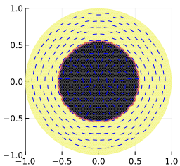
(a) $t=0.01$

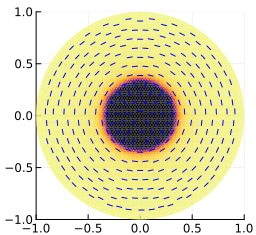
(b) $t=15$

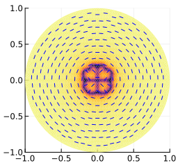
(c) $t=30$

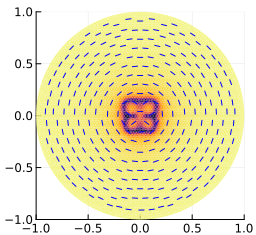
(d) $t=45$

(e) $t=60$

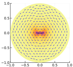
(f) $t=75$

(g) $t=90$

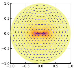
(h) $t=180$

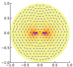
(i) $t=270$

Figure 1. Simulated evolution of a degree 1 tactoid, in which the initial and boundary conditions are defined by $\mathbf{n}_{0}=(-\sin\theta,\cos\theta)$ in (5.5).

5.3.2. Degree -1 tactoid

In the second trial, we take the director to wind in the reverse direction as the boundary of $\Omega$, by setting

(5.7) $$\mathbf{n}_{0}=\begin{pmatrix}-\cos\theta\\ \sin\theta\end{pmatrix}.$$

This leads to a tactoid of topological degree -1. In Figure 2, we observe that the tactoid shrinks in a radially asymmetrical way until it collapses into a vortex of degree -1, which eventually splits into two vortices of degree -1/2 that slowly move apart. Unlike the vortices in the previous experiment, these vortices have long V-shaped “tails” in which the scalar order parameter is small, and these tails persist as the vortices move.

(a) $t=0.01$

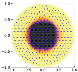
(b) $t=5$

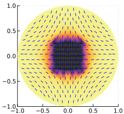
(c) $t=10$

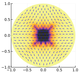
(d) $t=15$

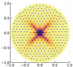
(e) $t=20$

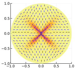
(f) $t=25$

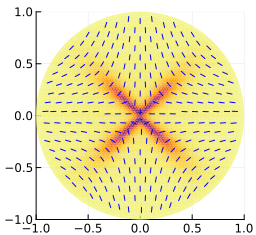
(g) $t=30$

(h) $t=60$

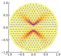
(i) $t=90$

Figure 2. Simulated evolution of a degree -1 tactoid, in which the initial and boundary conditions are defined by $\mathbf{n}_{0}=(-\cos\theta,\sin\theta)$ in (5.5).

5.3.3. Degree 0 tactoid

Finally, we take the constant director

(5.8) $$\mathbf{n}_{0}=\begin{pmatrix}1\\ 0\end{pmatrix},$$

leading to a tactoid of degree 0. As seen in Figure 3, this tactoid shrinks until it disappears entirely, leaving behind a uniform sample without vortices. As the tactoid shrinks, six “arms” emerge in the shape of an asterisk and persist longer than the surrounding tactoid, but we take this to be a side effect of the mesh structure.

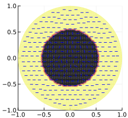
(a) $t=0.01$

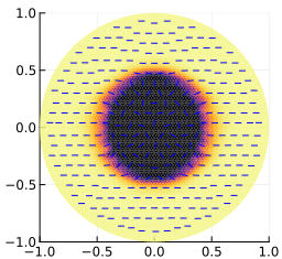
(b) $t=5$

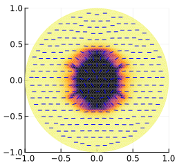
(c) $t=10$

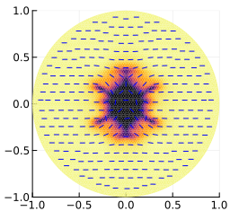
(d) $t=15$

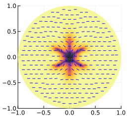
(e) $t=20$

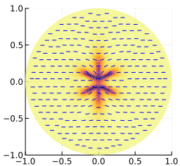
(f) $t=25$

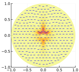
(g) $t=30$

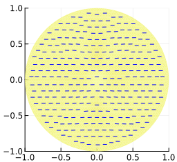
(h) $t=35$

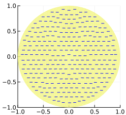
(i) $t=40$

Figure 3. Simulated evolution of a degree 0 tactoid, in which the initial and boundary conditions are defined by $\mathbf{n}_{0}=(1,0)$ in (5.5).

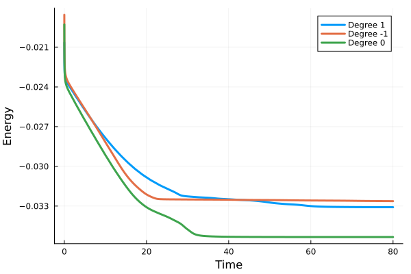
Figure 4. Energies of decaying tactoids over time for experiments outlined in Sections 5.3.1 (blue), 5.3.2 (orange), and 5.3.3 (green).

Appendix A Tensor calculus lemmas

Lemma A.1.

$|\mathrm{div}\,Q|^{2}\leq 3|\nabla Q|^{2}$ for all $Q\in\mathbb{R}^{3\times 3}$.

Proof.

(A.1) $$|\mathrm{div}\,Q|^{2} =\sum_{i=1}^{3}\left(Q_{i1,1}+Q_{i2,2}+Q_{i3,3}\right)^{2}$$

$$=\sum_{i=1}^{3}\left(Q_{i1,1}^{2}+Q_{i2,2}^{2}+Q_{i3,3}^{2}+2Q_{i1,1}Q_{i2,2}+2Q_{i1,1}Q_{i3,3}+2Q_{i2,2}Q_{i3,3}\right)$$

$$=\sum_{i=1}^{3}\left(3Q_{i1,1}^{2}+3Q_{i2,2}^{2}+3Q_{i3,3}^{2}-(Q_{i1,1}-Q_{i2,2})^{2}-(Q_{i1,1}-Q_{i3,3})^{2}-(Q_{i2,2}-Q_{i3,3})^{2}\right)$$

$$\leq\sum_{i=1}^{3}\left(3Q_{i1,1}^{2}+3Q_{i2,2}^{2}+3Q_{i3,3}^{2}\right)\leq 3|\nabla Q|^{2}$$

∎

Lemma A.2.

$|\mathrm{curl}\,Q|^{2}\leq 2|\nabla Q|^{2}$ for all $Q\in\mathbb{R}^{3\times 3}$.

Proof.

Here we take indices modulo 3 for simplicity; so, for example, $Q_{02,4}$ would mean $Q_{32,1}$.

(A.2) $$|\mathrm{curl}\,Q|^{2} =\sum_{i,j=1}^{3}(Q_{ji,(i+1)}-Q_{j(i+1),i})^{2}=\sum_{i,j=1}^{3}\left(2Q_{ji,(i+1)}^{2}+2Q_{j(i+1),i}^{2}-(Q_{ji,(i+1)}+Q_{j(i+1),i})^{2}\right)$$

$$\leq\sum_{i,j=1}^{3}\left(2Q_{ji,(i+1)}^{2}+2Q_{j(i+1),i}^{2}+2Q_{ji,i}^{2}\right)=2|\nabla Q|^{2}$$

∎

Lemma A.3.

$\left\lVert AB\right\rVert_{L^{2}}\leq 3\left\lVert A\right\rVert_{L^{\infty}}\left\lVert B\right\rVert_{L^{2}}$ for all $A\in L^{\infty}(\Omega;\mathbb{R}^{3\times 3}),B\in L^{2}(\Omega;\mathbb{R}^{3\times 3})$.

Proof.

(A.3) $$\left\lVert AB\right\rVert_{L^{2}}^{2} =\int_{\Omega}|AB|_{F}^{2}\,dx\leq\int_{\Omega}|A|_{F}^{2}|B|_{F}^{2}\,dx=\int_{\Omega}\left(\sum_{i,j=1}^{3}A_{ij}^{2}(x)\right)|B|_{F}^{2}\,dx$$

$$\leq\int_{\Omega}\left(9\max_{i,j,y}A_{ij}^{2}(y)\right)|B|_{F}^{2}\,dx=9\left\lVert A\right\rVert_{L^{\infty}}^{2}\left\lVert B\right\rVert_{L^{2}}^{2}$$

∎

References

- [1] S. Bartels. Numerical Methods for Nonlinear Partial Differential Equations. Springer International Publishing, Cham, 2015.
- [2] D. W. Berreman and S. Meiboom. Tensor representation of Oseen-Frank strain energy in uniaxial cholesterics. Phys. Rev. A, 30:1955–1959, Oct 1984.
- [3] J. P. Borthagaray, R. H. Nochetto, and S. W. Walker. A structure-preserving FEM for the uniaxially constrained Q-tensor model of nematic liquid crystals. Numer. Math., 145(4):837–881, 2020.
- [4] J. P. Borthagaray and S. W. Walker. The -tensor model with uniaxial constraint. In Geometric partial differential equations. Part II, volume 22 of Handb. Numer. Anal., pages 313–382. Elsevier/North-Holland, Amsterdam, 2021.
- [5] A. Braides. Local minimization, variational evolution and -convergence, volume 2094 of Lecture Notes in Mathematics. Springer, Cham, 2014.
- [6] Y. Cai, J. Shen, and X. Xu. A stable scheme and its convergence analysis for a 2D dynamic -tensor model of nematic liquid crystals. Math. Models Methods Appl. Sci., 27(8):1459–1488, 2017.
- [7] J. Castellano. Liquid Gold: The Story of Liquid Crystal Displays and the Creation of an Industry. World Scientific, 2005.
- [8] P. de Gennes and J. Prost. The Physics of Liquid Crystals. International Series of Monogr. Clarendon Press, 1995.
- [9] S. Dickmann. Numerische Berechnung von Feld und Molekülausrichtung in Flüssigkristallanzeigen. PhD thesis, Universität Karlsruhe (TH), 1995. Düsseldorf 1995. (Fortschritt-Berichte VDI. Reihe 20, Nr.155.) Fak. f. Elektrotechnik, Diss. v. 15.11.1994.
- [10] L. C. Evans. Partial differential equations, volume 19 of Graduate Studies in Mathematics. American Mathematical Society, Providence, RI, second edition, 2010.
- [11] L. C. Evans and R. F. Gariepy. Measure theory and fine properties of functions. Textbooks in Mathematics. CRC Press, Boca Raton, FL, revised edition, 2015.
- [12] F. C. Frank. I. Liquid crystals. On the theory of liquid crystals. Discussions of The Faraday Society, 25:19–28, 1958.
- [13] D. Golovaty, Y.-K. Kim, O. D. Lavrentovich, M. Novack, and P. Sternberg. Phase transitions in nematics: textures with tactoids and disclinations. Math. Model. Nat. Phenom., 15:8, 2020.
- [14] D. Golovaty, M. Novack, and P. Sternberg. A novel Landau–de Gennes model with quartic elastic terms. European J. Appl. Math., 32(1):177–198, 2021.
- [15] V. M. Gudibanda, F. Weber, and Y. Yue. Convergence analysis of a fully discrete energy-stable numerical scheme for the Q-tensor flow of liquid crystals. SIAM J. Numer. Anal., 60(4):2150–2181, 2022.
- [16] M. Hirsch and F. Weber. A Convergent Finite Element Scheme for the Q-Tensor Model of Liquid Crystals Subjected to an Electric Field. arXiv e-prints, page arXiv:2307.11229, July 2023.
- [17] R. Koizumi, D. Golovaty, A. Alqarni, B.-X. Li, P. J. Sternberg, and O. D. Lavrentovich. Topological transformations of a nematic drop. Science Advances, 9(27):eadf3385, 2023.
- [18] D. M. L. Longa and H.-R. Trebin. An extension of the Landau-Ginzburg-de Gennes theory for liquid crystals. Liquid Crystals, 2(6):769–796, 1987.
- [19] L. Longa and H.-R. Trebin. Structure of the elastic free energy for chiral nematic liquid crystals. Phys. Rev. A, 39:2160–2168, Feb 1989.
- [20] N. J. Mottram and C. J. P. Newton. Introduction to Q-tensor theory. arXiv e-prints, page arXiv:1409.3542, Sept. 2014.
- [21] C. Oseen. The theory of liquid crystals. Transactions of The Faraday Society, 29:883–899, 1933.
- [22] P.-O. Persson and G. Strang. A Simple Mesh Generator in MATLAB. SIAM Review, 46(2):329–345, 2004.
- [23] C. D. Schimming, J. Viñals, and S. W. Walker. Numerical method for the equilibrium configurations of a Maier-Saupe bulk potential in a Q-tensor model of an anisotropic nematic liquid crystal. Journal of Computational Physics, 441:110441, 2021.
- [24] I. W. Stewart. The static and dynamic continuum theory of liquid crystals: a mathematical introduction. CRC Press, 2019.
- [25] G. Van Der Zwan. On the tensor vs. the vector character of the director field in a nematic liquid crystal. Physica A: Statistical Mechanics and its Applications, 150(2):299–309, 1988.
- [26] E. G. Virga. Variational theories for liquid crystals, volume 8 of Applied Mathematics and Mathematical Computation. Chapman & Hall, London, 1994.
- [27] F. Weber and Y. Yue. On the convergence of an IEQ-based first-order semi-discrete scheme for the Beris-Edwards system. ESAIM Math. Model. Numer. Anal., 57(6):3275–3302, 2023.
- [28] J. Zhao, X. Yang, Y. Gong, and Q. Wang. A novel linear second order unconditionally energy stable scheme for a hydrodynamic Q-tensor model of liquid crystals. Computer Methods in Applied Mechanics and Engineering, 318:803–825, 2017.