Fast Shortest Path Polyline Smoothing With G1 Continuity and Bounded Curvature

Abstract

In this work, we propose a novel and efficient method for smoothing polylines in motion planning tasks. The algorithm applies to motion planning of vehicles with bounded curvature. In the paper, we show that the generated path: 1. has minimal length, 2. is $G^{1}$ continuous, and 3. is collision-free by construction, if the hypotheses are respected. We compare our solution with the state-of.the-art and show its convenience both in terms of computation time and of length of the compute path.

This work has been submitted to the IEEE for possible publication. Copyright may be transferred without notice, after which this version may no longer be accessible.

I Introduction

Motion planning is a fundamental task for many applications, ranging from robotic arm manipulation [12] to autonomous vehicle navigation [7]. The goal is to find a feasible (or optimal) path or trajectory to move an agent from a start to a target position, avoiding obstacles along the way.

When considering mobile robots subject to a minimum turning radius and moving at constant speed, the optimal path connecting two different configurations is given by Dubins curves [6]. When the robot has to travel across an area cluttered with obstacles, a popular strategy is to first identify a collision-free polyline joining an initial and a final configuration and then interpolate it by a smooth path (e.g., by a sequence of Dubins manoeuvres), which respect the kinematic constraint of the vehicle. Finding a good interpolation requires a good compromise between the computation time and quality of the resulting path. Some of the existing approaches, prioritise the quality of the path, but their high computational cost could make them unfit for real–time path generation [14]. Conversely, methods that prioritise computational efficiency can sometimes produce paths that lack formal mathematical properties or feasibility guarantees [2], compromising the quality of motion. Indeed, an important additional problem is that even if the initial polyline is guaranteed to be collision free, this is not necessarily true for the interpolated path.

In this paper, we propose the Dubins Path Smoothing (DPS) algorithm, a novel solution designed to achieve a fast interpolation of a polyline with a sequence of motion primitives respecting $G^{1}$ continuity and bounded curvature constraint. An example output of the algorithm is in Figure 1, where a polyline of points, shown in blue, is approximated by a sequence of Dubins manoeuvres (in red) respecting the non-holonomic constraint of the mobile robot.

Figure 1: In blue the original 4-points polyline $P=\{p_{0},\ldots,p_{3}\}$ and in red the smoothed path from DPS.

The key findings of the paper are the following: 1. the length of the interpolated path is upper bounded by that of the polyline; 2. under some assumptions on the polyline, the interpolated path is guaranteed to be collision-free if the polyline is also collision-free, 3. the solution is robust: if we cut away some pieces of the solution, the remaining segments are not affected; 4. given some constraints on the construction of the smoothed path, we prove its optimality, i.e., it is the shortest one; 5. since the computed path is a combination of segments and arcs of circle, then an offset of the solution is a path with the same characteristics and curve primitives. This is a fundamental property for tasks such as CNC where the set of available curve-classes is restricted.

In the paper, we describe the algorithm and offer a comprehensive theoretical analysis supporting the aforementioned claims. In addition, we provide both a sequential and parallel implementation of the algorithm and show its efficiency and effectiveness against existing methods. Finally, we report our experimental results derived from its execution with a real robot with limited hardware to show in a concrete use-case its computational efficiency.

The remainder of this paper is structured as follows. In Section II, we present a review of the state of the art on algorithms for interpolation and approximation of polylines. In Section III, we detail the tackled problem and in Section IV we show the proposed algorithm, also providing formal mathematical support to the claims. The experimental results and the performance evaluation are presented in Section V, and in Section VI we discuss the potential algorithm applications, limitations, and future work.

II Related Work

Nonholomic vehicles cannot follow a series of segments as in a polyline, but instead must find a combination of smoothly joint segments to correctly follow the path.

The problem of finding the shortest path with $G^{1}$ continuity to go from an initial position to a final one, with fixed initial and final orientation and also fixed minimum turning radius, was formalized in [15] and the solution was formulated in [6], now known as the Markov-Dubins path.

A generalization of the problem, in which the goal is to interpolate multiple points, is called the Multi-Point Markov-Dubins Problem (MPMDP) [7, 14]. Some works have focused on optimal control formulations [14, 9], which are then computed using Non-Linear Programming solvers [14], or Mixed-Integer Non-Linear Programming ones [8]. While this approach allows for finding precise solutions, it also comes with considerable computational costs and it may not converge, hence not find a solution. A different approach is presented in [8], in which the authors sample possible angles for each waypoint and, by exploiting dynamic programming and refinements on the solutions, they are able to compute the path with great precision and low computational costs. An extension to their work allows for using GPGPUs in order to parallelize the computation and further improve performance [21].

A related subproblem that has gained a lot of traction is the 3-Points Dubins Problem (3PDP) [9, 22], which is a sub-problem of the MPMDP focusing on interpolating 3 points with only the middle angle unknown. It can be used to change parts of the interpolated problem by inserting another point and connecting the previous and next node to the new one, while not changing the rest of the path.

Previous work has dealt also with the MPMDP by proposing solutions which embed in the same procedure both the sampling of the points and the following interpolation based on Dubins curve. In [5], the authors propose an approach based on a modified essential visibility graph, in which they connect circles centered in the obstacles’ vertexes. Similarly, in [29], the authors construct a so called Dubins path graph to hold all the different pieces of all the possible solutions, and then they run Dijkstra algorithm on a weight matrix to find the shortest path. In [24], the authors propose a revisited A* algorithm, which takes into account the nonholonomic constraints. This new implementation of A* is applied to a weighted graph which represents the scenario by interpolating a Dubins path between each node and obstacle. A combined solution for point sampling, using RRT*, and interpolation with Dubins curves is proposed in [11]. A post-process algorithm prevents possible collisions from happening during the interpolation step by computing a Dubins path pairwise considering the initial and final angles aligned with the segments that form the path obtained from RRT*. A modified version of RRT* that takes into account nonholonomic constraints is proposed in [32]. Here, the authors implemented an RRT* version that creates the Dubins path together with the sampling itself; this is achieved by connecting each new point with a feasible Dubins curve rather than a straight line as in classic RRT*. Similarly, in [27], the points are sampled in the 3D space from which the Dubins curves are directly created, representing feasible flight procedures defined by the International Civil Avionics Organization.

Focusing on the problem of fitting (or smoothing) a polyline, an approach similar to our was presented in [31], in which the authors propose an algorithm with complexity $O(n^{2})$ to smooth the polyline by first finding maximum convex subsections of the polyline and then approximating them with curves. Another analogous approach was presented in [2], in which the authors use Fermat Spirals to approximate the polyline with a series of differentiable curves, providing an easy to follow path for UAVs and UMVs. While these approaches may provide good approximations minimizing variations in the curvature, based on the theoretical complexity presented, they are not as performing as ours, and they lack a formal proof of correctness and optimality. In recent times, it was shown that a curvilinear coordinate transformation could be used to iteratively adapt the polyline to the reference frame [28]. The authors consider the polyline as the control polygon of a B-spline, which is then iteratively refined in conjunction with a sampling step, in order to reduce the curvature and smooth a $C^{2}$. Nevertheless, the authors neither consider shortest paths, nor guarantee curvature bound.

A final comparison can be made with biarcs [1], which provide a fast solution to a similar problem of fitting points given an initial and final angles with $G^{1}$ continuity. However, they do not consider bounded curvature nor minimize the length of the solution.

III Problem Statement

In this section, we provide the problem statement and show a sub-problem, which can be solved, without loss of generality, exploiting the Bellman’s principle of optimality.

Figure 2: Visual representation of the standard placement for the 3-points sub-problem.

Definition 1 (Polyline).

A polyline $P=(p_{0},p_{1},\ldots,p_{n-1})$ is an ordered sequence of $n>2$ points $p_{j}=(x_{j},y_{j})\in\mathbb{R}^{2}$.

Assumption 1 (Conditions on the polyline).

Any triplet of consecutive points $p_{j-1},p_{j},p_{j+1}$ of the polyline $P$ is not-aligned, and, given a scenario with obstacles, the polyline $P$ is collision-free w.r.t. the obstacles by design (e.g., given by RRT* [13]).

We will later provide a formal proof of the minimum size of which the obstacles should be inflated in order to produce a collision-free polyline $P$ as in Assumption 1.

Definition 2 (Problem).

Let $P$ be a collision-free polyline. The goal is to find a feasible path $\mathcal{P}$ approximating the polyline $P$ with a shortest path for a non-holonomic robot subject to a minimum turning radius $r$, respecting $G^{1}$ continuity.

We define the angles

$$\theta_{j}=\mathrm{atan2}(y_{j+1}-y_{j},x_{j+1}-x_{j}),\quad j<n-1$$

as the direction between point $p_{j}$ and point $p_{j+1}$, and

$$\alpha_{j}=\pi-(\theta_{j}-\theta_{j-1})$$

as the internal angle formed between $\overrightarrow{p_{j-1}p_{j}}$ and $\overrightarrow{p_{j}p_{j+1}}$, as in Figure 2.

To tackle the problem, without loss of generality, we can consider the sub-problem of finding an approximate path $Q$ with $G^{1}$ continuity and bounded curvature for 3 consecutive non-aligned points $p_{i},p_{m},p_{f}$ (respectively initial, middle and final points). When they are aligned, the solution coincides with the polyline itself. To solve this problem, we construct the circle of fixed radius $r$ tangent to the two lines defined by the polyline $\{p_{i},p_{m},p_{f}\}$, as shown in Figure 2. This intersection defines the tangent points $q_{m_{1}}$ and $q_{m_{2}}$ in proximity of point $p_{m}$.

Considering sub-problems composed of 3 points allows for an easier and more efficient computation of the approximate path, since each sub-problem can be solved separately and hence computed in parallel.

We want to construct the shortest path with $G^{1}$ continuity and bounded curvature interpolating with line segments and circular arcs the sequence of ordered points $Q=(p_{i},q_{m_{1}},q_{m_{2}},p_{f})$ shown in Figure 2. The designed path is feasible for a non-holonomic robot to follow by construction. Indeed, every arc $\widearc{q_{m_{1}}q_{m_{2}}}$ is from a circle with the radius equal to the minimum turning radius $r$ of the robot, and the arrival angle, after every arc, corresponds to the slope of the next straight segment in the path. The $G^{1}$ continuity condition and the bounded curvature enable the robot to navigate the constructed path.

It is important to notice that the segments between the points of $P$ must be long enough to contain the tangent points in the correct order. For instance, in the case of Figure 2, the segment $\overline{p_{i}p_{m}}$ must be longer than the segment $\overline{q_{m_{1}}p_{m}}$. We ensure this in Lemma 2.

IV Solution formalization

In this section, we will formalize the 3-points sub-problem and its solution. In order to ease the following demonstration, without loss of generality, we shall translate and rotate the initial configuration for the 3-points sub-problem. We start by shifting the points by the coordinates of $p_{i}$, bringing it to the origin, then we apply a rotation $R(\varphi)$ to bring the point $p_{m}$ to the positive $x$-axis. If $p_{f}$ is below the $x$-axis ($y_{f}<0$), we reflect it on the $x$-axis and consider it positive.

Lemma 2 (Existence constraint).

Let $P=(p_{i},p_{m},p_{f})$ be a polyline of 3 non aligned points, and $\alpha_{m}$ the angle in $p_{m}$, as in Figure 2. The following constraint must be satisfied to ensure the existence of a $G^{1}$ approximation of the polyline:

$$\min\left(\lvert\lvert p_{m}-p_{i}\rvert\rvert,\lvert\lvert p_{f}-p_{m}\rvert\rvert\right)\geq\frac{r}{\tan(\alpha_{m}/2)}.$$ (1)

Proof.

In the standard setting, the angle $\alpha_{m}$ is equal to:

$$\alpha_{m}=\pi-\theta_{m},\quad\theta_{i}=0.$$

The two triangles $\overset{\triangle}{q_{m_{1}}p_{m}C}$ and $\overset{\triangle}{q_{m_{2}}p_{m}C}$ are congruent since they have three congruent edges, namely $r$, $d$, which they share, and $l$, which is $l=\sqrt{d^{2}-r^{2}}$.

Since,

$$r=d\sin{\frac{\alpha_{m}}{2}},\quad l=d\cos{\frac{\alpha_{m}}{2}},$$ (2)

it follows that:

$$l=\frac{r}{\tan(\alpha_{m}/2)},\quad d=\frac{r}{\sin(\alpha_{m}/2)}.$$ (3)

Consequently, the tangent points are:

$$q_{m_{1}}=(x_{m}-l,0),\quad q_{m_{2}}=(x_{m}+l\cos{\theta_{m}},\leavevmode\nobreak\ l\sin{\theta_{m}}),$$

and, it must hold that:

$$\begin{cases}l\leq x_{m}\\ l\leq||p_{f}-p_{i}||\end{cases},$$

meaning that the tangent points are within the segments of the polyline.

Finally, $\alpha_{m}\in\{0,\pi\}$ makes the denominator of Equation 1 vanish, but this situation corresponds to aligned points, which is excluded by Assumption 1. ∎

In the general case, when considering the whole polyline $P$, we also must ensure that the tangent points in the segment $\overline{p_{j}p_{k}}$ exist and are consecutive, that is, $||p_{j}-q_{j_{2}}||\leq||p_{j}-q_{k_{1}}||$ and $||p_{k}-q_{k_{1}}||\leq||p_{k}-q_{j_{2}}||$.

Corollary 3 (Global existence condition).

From Lemma 2, a solution exist if, for every two consecutive points $p_{j},\,p_{k}\in P$, the following constraint is also satisfied:

$$||p_{j}-p_{k}||\geq\left\lvert\frac{r}{\tan(\alpha_{j}/2)}\right\rvert+\left\lvert\frac{r}{\tan(\alpha_{k}/2)}\right\rvert.$$ (4)

Corollary 4 (Tangent points).

If the constraints in Lemma 2 and Corollary 3 are satisfied, then the tangent points $q_{j_{1}},q_{j_{2}}$ between the circle and the vectors $v_{j_{1}}=\overrightarrow{p_{j-1}p_{j}}$ and $v_{j_{2}}=\overrightarrow{p_{j}p_{j+1}}$ in the general position exist and are given by:

$$\begin{array}[]{rcl}q_{j_{1}}&=&p_{j}-l_{j}\hat{v}_{j_{1}},\\ q_{j_{2}}&=&p_{j}+l_{j}\hat{v}_{j_{2}}\end{array},$$ (5)

where $\hat{v}_{j_{1}}$ is the direction from $p_{j-1}$ to $p_{j}$, and $\hat{v}_{j_{2}}$ the direction from $p_{j}$ to $p_{j+1}$.

Our DPS algorithm generates a path that does not interpolate $P$, but it is possible to derive an upper bound of its distance from $P$.

Corollary 5 (Distance from the polyline points).

The path $Q$ has distance $D_{j}$ from the intermediate point $p_{j}$ of the polyline $P$ given by:

$$D_{j}=d-r=r\left(\frac{1}{\sin(\alpha_{m}/2)}-1\right)=r\cdot\text{excsc}(\alpha_{m}/2)$$ (6)

The lemma and its corollaries are implemented in Algorithm 1, which runs in constant time.

1:function solve_3_points($p_{i}=(x_{i},y_{i})$, $p_{m}=(x_{m},y_{m})$, $p_{f}=(x_{f},y_{f})$)

2:     $v_{1}\leftarrow[x_{m}-x_{i},y_{m}-y_{i}]^{T}$

3:     $v_{2}\leftarrow[x_{f}-x_{m},y_{f}-y_{m}]^{T}$

4:     $\hat{v_{1}}\leftarrow v_{1}/||v_{1}||$

5:     $\hat{v_{2}}\leftarrow v_{2}/||v_{2}||$

6:     $l=r\dfrac{||v_{1}\times v_{2}||}{(v_{1}\cdot v_{2})+||v_{1}||\,||v_{2}||}$

7:     $q_{m_{1}}\leftarrow p_{m}-l\hat{v_{1}}$

8:     $q_{m_{2}}\leftarrow p_{m}+l\hat{v_{2}}$

9:     $Q\leftarrow\left\{\overline{p_{i}q_{m_{1}}}+\widearc{q_{m_{1}}q_{m_{2}}}\right\}$

10:    return $Q$

Algorithm 1 The pseudo-code to compute the $i^{\text{th}}$ piece of the path $\mathcal{P}$ (i.e., $Q_{i}$), in the general case.

On the complexity of the algorithm. Since the computation of each individual segment of the path can be performed in constant time, the overall complexity of the algorithm to compute all $n-1$ segments of the polyline $P$ is linear with respect to the number of points $n$. Since every time a new problem is provided, each segment of the path must be computed, the algorithm’s complexity is bounded by $n$ in both the best and worst cases. Therefore, the algorithm operates in $\Theta(n)$ time.

Figure 3: In red, an example of the J Dubins path type in the standard setting used in Theorem 7.

Assumption 6 (Minimum distance between points).

Let $r$ be the minimum turning radius of the robot, $p_{j}$ and $p_{k}$ two consecutive points of the polyline $P$ and $q_{k_{2}}$ the first tangent point after $p_{k}$. We assume that the points $p_{j}$ and $q_{k_{2}}$ have a distance of at least $4r$:

$$||p_{j}-q_{k_{2}}||\geq 4r.$$

Based on this assumption, we now prove that our solution has length optimality.

Theorem 7 (Optimality of $\mathbf{Q}$).

The path $Q$ is a Dubins path, i.e., the shortest one of bounded curvature and $G^{1}$ continuity.

Proof.

Using the principle of Bellman, it is possible to consider the sub-problem of showing the optimality of the sub-path given by three points $p_{i},q_{m_{1}},q_{m_{2}}$, see Figure 3. If the theorem holds for the sub-problem, then it holds also for the whole path $Q$.

In order to do so, we show that the path $p_{i},q_{m_{1}},q_{m_{2}}$ is a Dubins path, i.e., the shortest one connecting with $G^{1}$ continuity and bounded curvature the points $p_{i}$ with angle $\theta_{i}$ and $q_{m_{2}}$ with angle $\theta_{m}$. The $G^{1}$ continuity and the bounded curvature are given by construction, and now we prove the length optimality.

To take advantage of the Dubins formulation, we need to recast the problem to Dubins standard setting, i.e., bringing the initial and final points ($p_{i}$ and $q_{m_{2}}$, respectively) on the $x$-axis with $p_{i}$ in the origin. Without loss of generality, we first perform a translation of the points so that $p_{i}$ is on the origin. Then, we rotate the points so that $q_{m_{2}}$ is on the positive $x$-axis, and finally we scale the points so that the radius is unitary, as in [20].

We can now show that our path is a path of type J, that is, a path composed of a straight line and a circle.

Dubins paths can be in the form of CSC, i.e., formed by a circle arc followed by a straight segment and finally by another circle arc, or in the form CCC, i.e., with three circle arcs [23]. Assumption 6 rules out the cases CCC, hence we have to consider CSC cases only. Starting from a CSC Dubins path, we show the condition for which the first arc has length $\ell_{1}=0$. We use formulas (13) and (19) of  [20], herein adapted to our notation:

$$0=\ell_{1}=|\vartheta_{S}-\theta_{i}|\,\text{mod}2\pi,$$

which happens when the angle of the line segment $\vartheta_{S}$ is equal to the initial angle $\theta_{i}$, in other words, when $\vartheta_{S}=\theta_{i}$. This immediately implies that the final arc has length $\ell_{3}$ given by:

$$\ell_{3}=|\theta_{m}-\vartheta_{S}|\,\text{mod}2\pi=|\theta_{m}-\theta_{i}|=|\pi-\alpha|,$$

which is in agreement with the presented construction. It remains to show that also the length of the straight line segment is the same in Dubins’ formula as well as in our construction. The length of the line segment $\ell_{2}$ from [20] is given by substituting $\vartheta_{S}=\theta_{i}$:

$$\ell_{2}=\left(||p_{i}-p_{m}||-\sin\theta_{m}\right)\cos\theta_{i}+\sin\theta_{i}\cos\theta_{m},$$

which is simplified with trigonometric manipulations to:

$$\ell_{2}=||p_{i}-p_{m}||\cos\theta_{i}-\sin(\theta_{m}-\theta_{i}).$$

We have to prove that $\ell_{2}=||p_{i}-q_{m_{1}}||$, that is, that the optimal Dubins length is the same as the length of our construction, so that the two perfectly match. We first note that $||p_{i}-p_{m}||\cos(\theta_{i})$ corresponds to the segment $||p_{i}-H||$ of Figure 3, hence it remains to show that $||q_{m_{1}}-H||=\sin(\theta_{m}-\theta_{i})$, the latter being equal to $\sin(\pi-\alpha)=\sin\alpha$. The length of the height $h=||q_{m_{2}}-H||$ is on one hand $h=\ell\sin\alpha$, on the other hand we have $h=||q_{m_{1}}-q_{m_{2}}||\cos(\alpha/2)$. Combining the latter two relations, we get

$$\begin{array}[]{rcl}||q_{m_{1}}-H||&=&||q_{m_{1}}-q_{m_{2}}||\sin(\alpha/2)\\[6.99997pt] &=&\displaystyle l\sin(\alpha)\frac{\sin(\alpha/2)}{\cos(\alpha/2)}\\[8.00003pt] &=&\displaystyle\frac{r}{\tan(\alpha/2)}\sin\alpha\tan(\alpha/2)\\[8.00003pt] &=&r\sin\alpha,\end{array}$$

and since, by hypothesis and without loss of generality, $r=1$, we proved that $||q_{m_{1}}-H||=\sin\alpha$ and thus that our construction is a Dubins path. ∎

Corollary 8 (Optimality of $\mathcal{P}$).

Provided Corollary 5 and Theorem 7, and assuming the points $p_{j}\in P$ satisfy Corollary 3, the concatenation of the paths $Q_{i}$ forming $\mathcal{P}$ is the shortest path with distance $D_{j}$ or less from point $p_{j}$ and with bounded turning radius and $G^{1}$ continuity.

Now, we show the minimum offset required to enlarge the obstacles when using motion planning algorithms, such as visibility graphs [16] and RRT* [13], to create a road-map to ensure a collision free path with DPS. In order to do so, we shall consider the visibility graph algorithm, in which the road-map is constructed between the vertexes of the polygons representing the (inflated) obstacles. The resulting polyline, is by construction the closest polyline to the obstacles and hence any other polyline not crossing the (inflated) obstacles, will be collision free.

Figure 4: A scenario in which the mitered offset $O$, in purple, is larger than the radius of the robot $h$ in orange. In blue, the turning radius of the robot and in green the path.

Assumption 9 (Convex obstacles).

The obstacles present in the map are convex. If the obstacles are not convex, a convex hull can be employed to enable Theorem 10.

Theorem 10 (Sufficient condition for a collision-free path).

Let $h$ be the radius of the robot, $r$ the minimum turning radius and $\alpha_{m}$ the angle at the vertex $v$ of a convex obstacle, as shown in Figure 4. The path $Q$, in green, is collision-free if the obstacles in the environment are subject to a mitered offset [4, 30, 17] $O$ of at least:

$$O=\max\left(h\sin\frac{\alpha_{m}}{2}+r\left(1-\sin\frac{\alpha_{m}}{2}\right),\leavevmode\nobreak\ h\right).$$ (7)

Proof.

The goal is to find an offset $O$ such that the path $Q$, is always collision-free, i.e., the following constraints are satisfied along the whole path:

$$\begin{cases}O>h\\ ||v-w||>h\end{cases}.$$ (8)

Since we are considering a mitered offset, the offset $O$ is the radius of a circle with center on the vertex $v$ of the obstacle, as shown in Figure 4.

We can write the second constraint of Equation 8 in terms of $r$ and $O$:

$$||v-w||=\frac{O}{\sin\left(\alpha_{m}/2\right)}-(||c-p_{m}||-r),$$

where the value $||c-p_{m}||$ is $d$ from Equation 3, which can be expressed in function of $r$:

$$\begin{array}[]{rcl}||v-w||&=&\dfrac{O}{\sin\left(\alpha_{m}/2\right)}-\dfrac{r}{\sin(\alpha_{m}/2)}+r\\ &=&\dfrac{O}{\sin\left(\alpha_{m}/2\right)}-r\left(\dfrac{1}{\sin(\alpha_{m}/2)}-1\right)>h.\end{array}$$

By solving for the offset $O$, we have:

$$O>h\sin\frac{\alpha}{2}+r\left(1-\sin\frac{\alpha_{m}}{2}\right).$$ (9)

Finally, the offset must be the maximum value between 9 and $h$. ∎

Lemma 11 ($\mathbf{Q}$ is shorter than $\mathbf{P}$).

The path $Q$ has a total length that is less than the length of the polyline $P$.

Proof.

To show that this is true, we must show that the arc of circle is shorter than reaching the point of the polyline and going back:

$$|\widearc{q_{m_{1}}q_{m_{2}}}|=r(\pi-\alpha)\leq 2l.$$

From Equation 3, it follows that:

$$\pi-\alpha\leq\frac{2}{\tan(\alpha/2)},$$

which is always true for values of $\alpha\in[0,\pi)$. If $\alpha=\pi$, then the three points are aligned, which is excluded by Assumption 1.

∎

V Experimental Results

(a) Tests run on a desktop PC.

(b) Tests run on an embedded system.

Figure 5: Performance comparison of the proposed algorithm, OMPL, and MPDP in path interpolation tasks.

In this section, we present a thorough experimental evaluation of the proposed algorithm. The experiments were conducted on a desktop computer with an Intel i9-10940X processor and an Nvidia RTX A5000 GPU, running Ubuntu 22.04. We divide the tests in different sections in order to highlight the strengths and the weaknesses of our approach compared to the state-of-the-art.

V-A Path Interpolation

In this first experiments, we want to show the performance improvement that our algorithm brings over the state of the art  [7, 1] both for computation times and for the lengths of the approximated path over interpolation. To do so, we fit $N=10^{i},i\in\{1\ldots 6\}$ points randomly sampled and repeat the tests 1000 times. We show the average time values in Figure 5 and the average lengths in Table I.

The points are each time sampled on a circle whose center is the previous point and whose radius is uniformly extracted in $[1,10]$, in such a way that the constraints, shown in Section IV, are satisfied.

We show the performance of our approach in comparison to two state-of-the-art algorithms: the Open Motion Planning Library (OMPL) [26] and the iterative algorithm introduced in [8] that uses dynamic programming to interpolate multiple points with Dubins paths, hereafter referred to as MPDP. There are noteworthy differences between our approach and these algorithms:

• OMPL does not support direct interpolation of multiple points, therefore, we exploit DPS to compute the intermediate points $q_{i}$ and angles $\theta_{i}$, which OMPL then uses to interpolate the path with Dubins manoeuvres.

• MPDP is a sampling-based algorithm designed to interpolate points precisely by finding an approximation of the optimal angles, ensuring that the final path passes through each point. Our algorithm instead focuses on finding shorter paths by not passing though the points, while maintaining a bounded distance and $G^{1}$ curvature continuity.

We implement and evaluate two versions of our algorithm: sequential and parallel, which is possible since the paths between triplets of points are independent, as discussed in Section IV. The parallel version is implemented in CUDA and is distributed on all the GPU cores available.

Figure 5(a) shows that our algorithm (both sequentially and in parallel, respectively DPS-Seq and DPS-Par) outperforms in computational times OMPL by approximately one order of magnitude and MPDP by two orders of magnitude. After an initial setback, the parallel implementation (DPS-Par) surpasses OMPL by one order of magnitude and MPDP by two orders of magnitude as the number of interpolated points increases. The initial lack of performance improvement in the parallel implementation is attributed to the time required to transfer data between CPU and GPU memory, which exceeds the time required for the actual computations of fewer points. For this experiment, we compare also to the biarc [1] implementation. Indeed, biarcs have characteristics similar to the approach we propose, since they are $G^{1}$ curves with lines and circles, but they do not constrain the curvature nor minimize lengths in that form. From a performance aspect, our implementation appears to be faster and also shorter, as shown in Table I.

We also run the same tests on a Nvidia AGX Xavier, which is an embedded system frequently used in automotive. Figure 5(b) shows that our algorithm DPS maintains the gain in performance shown in Figure 5(a).

# of points	DPS	MPDPP	MPDPQ	OMPL	Biarcs
$10^{1}$	1	1.040	1	1	1.11
$10^{2}$	1	1.090	1	1	1.22
$10^{3}$	1	1.085	1	1	1.21
$10^{4}$	1	1.086	1	1	1.21
$10^{5}$	1	1.086	1	1	1.21
$10^{6}$	1	1.086	1	1	1.21

Table I: The ratio between the lengths found using the different algorithms against the lengths found with the sequential algorithm. MPDP_P runs through the points $p$ of the polyline $P$, whereas MPDP_Q runs through the tangent points found using our approach.

Figure 6: The results of the experiments run on the visibility graphs showing the times to achieve a solution given the length of the path found on the visibility graph.

In Table I, we experimentally validate that the paths obtained are actually a concatenation of Dubins manoeuvres. Indeed, while MPDP yields longer paths by passing through the points $p_{j}$ of the polyline (column MPDP_P), if we use it to interpolate the tangent points (column MPDP_Q), then we obtain the same path, showing that the path we obtain is indeed optimal. An identical result, is observed by running OMPL through the tangent points and their angles, giving also an experimental validation of the length optimality.

V-B Road Maps

In this experiment, we evaluate the performance of our algorithm DPS in computing a feasible path using a visibility graph on maps with obstacles chosen from [25].

For this experiment, we first construct the visibility road map [16] by considering the vertices of the inflated obstacles (as described in Theorem 10), then we use A* to compute the shortest path on the road map and finally we interpolate using our algorithm. We compare our approach to MPDP, to which we must feed the extracted polyline, and to OMPL to which we have to pass the tangent points and their angles, as before.

The experiments were run on 10000 different couples of points, for statistical analysis. In Figure 6, the results show that, even when the number of points is low, our algorithm greatly outperforms the competitors. Moreover, the paths that are extracted are feasible to be followed by construction, as proven in Theorem 10.

V-C Path Sampling Interpolation

Figure 7: The number of successful cases out of 500 tests at different timeouts.

In this experiment, we compare three approaches based on RRT* [13]. First, we use the standard RRT* implementation available in OMPL as a baseline, applying it for both sampling the points and interpolating the shortest path with Dubins. Next, we present the results for OMPL-DPS, where points are still sampled using the RRT* implementation from OMPL, but the shortest path is approximated using our approach. Finally, we introduce RRT*-DPS, which involves a standard implementation of RRT* from [13] coupled with our algorithm. It’s important to note that our RRT* implementation does not incorporate heuristic functions or path smoothing (as done by OMPL). However, we employ a 1% tolerance relative to the map size to reach the goal more cleanly. This approach, not used by OMPL, may offer a speed advantage over the other approaches.

In order for RRT* to terminate, we need to specify a timeout. The experiment consisted in varying the number of timeouts in $\{0.05,0.1,0.2,0.5,1,2\}$s, and, for every timeout, we randomly sampled 100 pairs of initial and final points and tested the algorithms. The sampled pairs were run 5 times each and the results shown in Figure 7 are the average values. Our algorithm manages to keep up with the state-of-the-art and outperforms the baseline in multiple timeouts.

It is worth noticing that the bottleneck of path approximation via sampling based methods is the algorithm for sampling. Indeed, when we substitute RRT* from OMPL with a lighter implementation, the performance improvements are notable even for smaller timeouts. While this is indeed expected, the results still show that we are able to reduce the lengths of the paths, while yet maintaining a success rate as high as the one obtain by the state-of-the-art or even surpassing it.

V-D Physical Robot Experiment

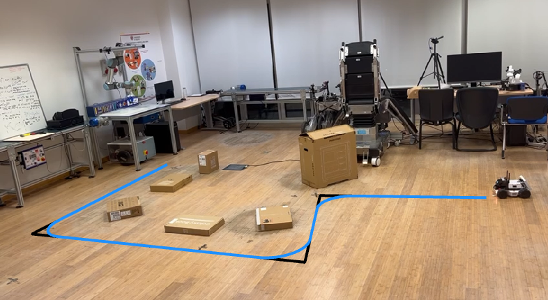
Figure 8: In black, the initial polyline $P$ that the robot was supposed to follow. In blue, the smoothed path $\mathcal{P}$ computed with DPS and followed.

Finally, we briefly showcase an example of our algorithm used in a real scenario by a robot to move smoothing a polyline between obstacles.

For the experiment, we used a car-like vehicle named Agilex Limo, driven with the four-wheel differential mode. We embedded the DPS algorithm implementation in a ROS2 node, which sends command velocity messages to the robot. The lightweight computational requirements to solve the DPS algorithm enables also the Nvidia Jetson Nano, an embedded computer used onboard by the robot, to swiftly find a solution.

VI Conclusion

We have presented DPS, a fast algorithm to generate the shortest smooth approximation of a polylines with $G^{1}$ continuity and bounded curvature.

This approach comes with a series of important proved properties, i.e, proofs and conditions on existence, optimality, feasibility, and bounded distance, enabling not only to find an optimal approximation for the path, but also to ensure the quality of such path.

As a future work, we aim at enabling higher levels of curvature continuity, i.e., $G^{2}$ with clothoids or $G^{3}-G^{4}$ with intrinsic splines.

References

- [1] Enrico Bertolazzi and Marco Frego. A Note on Robust Biarc Computation. Computer-Aided Design and Applications, 16(5):822–835, 2019.
- [2] Xiao Chen, Jianqiang Zhang, Min Yang, Liu Zhong, and Jiao Dong. Continuous-Curvature Path Generation Using Fermat’s Spiral for Unmanned Marine and Aerial Vehicles. In 2018 Chinese Control And Decision Conference (CCDC), pages 4911–4916, 2018.
- [3] Zheng Chen and Tal Shima. Shortest Dubins paths through three points. Automatica, 105:368–375, 2019.
- [4] B.K. Choi and S.C. Park. A pair-wise offset algorithm for 2D point-sequence curve. Computer-Aided Design, 31(12):735–745, 1999.
- [5] Egidio D’Amato, Immacolata Notaro, and Massimiliano Mattei. Reactive Collision Avoidance using Essential Visibility Graphs. In 2019 6th International Conference on Control, Decision and Information Technologies (CoDIT), pages 522–527, 2019.
- [6] L. E. Dubins. On Curves of Minimal Length with a Constraint on Average Curvature, and with Prescribed Initial and Terminal Positions and Tangents. American Journal of Mathematics, 79(3):497–516, 1957.
- [7] Marco Frego, Paolo Bevilacqua, Stefano Divan, Fabiano Zenatti, Luigi Palopoli, Francesco Biral, and Daniele Fontanelli. Minimum time—Minimum jerk optimal traffic management for AGVs. IEEE Robotics and Automation Letters, 5(4):5307–5314, 2020.
- [8] Marco Frego, Paolo Bevilacqua, Enrico Saccon, Luigi Palopoli, and Daniele Fontanelli. An Iterative Dynamic Programming Approach to the Multipoint Markov-Dubins Problem. IEEE Robotics and Automation Letters, 5(2):2483–2490, 2020.
- [9] Xavier Goaoc, Hyo-Sil Kim, and Sylvain Lazard. Bounded-Curvature Shortest Paths through a Sequence of Points Using Convex Optimization. SIAM Journal on Computing, 42(2):662–684, 2013.
- [10] Xavier Goaoc, Hyo-Sil Kim, and Sylvain Lazard. Bounded-Curvature Shortest Paths through a Sequence of Points Using Convex Optimization. SIAM Journal on Computing, 42(2):662–684, 2013.
- [11] Hung Hoang, Anh Khoa Tran, Lam Nhat Thai Tran, My-Ha Le, and Duc-Thien Tran. A Shortest Smooth-path Motion Planning for a Mobile Robot with Nonholonomic Constraints. In 2021 International Conference on System Science and Engineering (ICSSE), 2021.
- [12] Keunwoo Jang, Sanghyun Kim, and Jaeheung Park. Motion Planning of Mobile Manipulator for Navigation Including Door Traversal. IEEE Robotics and Automation Letters, 8(7):4147–4154, 2023.
- [13] Sertac Karaman and Emilio Frazzoli. Sampling-based algorithms for optimal motion planning. The international journal of robotics research, 30(7):846–894, 2011.
- [14] C Yalçın Kaya. Markov–dubins interpolating curves. Computational Optimization and Applications, 73(2):647–677, 2019.
- [15] Andrey Andreyevich Markov. Some examples of the solution of a special kind of problem on greatest and least quantities. Soobshch. Karkovsk. Mat. Obshch, 1:250–276, 1887.
- [16] Hanlin Niu, Al Savvaris, Antonios Tsourdos, and Ze Ji. Voronoi-visibility roadmap-based path planning algorithm for unmanned surface vehicles. Journal of Navigation, 72(4):850–874, 2019.
- [17] Sang C. Park and Yun C. Chung. Mitered offset for profile machining. Computer-Aided Design, 35(5):501–505, 2003.
- [18] Gianfranco Parlangeli. Shortest paths for Dubins vehicles in presence of via points. IFAC-PapersOnLine, 52(8):295–300, 2019. 10th IFAC Symposium on Intelligent Autonomous Vehicles IAV 2019.
- [19] Gianfranco Parlangeli, Daniela De Palma, and Rossella Attanasi. A novel approach for 3PDP and real-time via point path planning of Dubins’ vehicles in marine applications. Control Engineering Practice, 144:105814, 2024.
- [20] Mattia Piazza, Enrico Bertolazzi, and Marco Frego. A Non-Smooth Numerical Optimization Approach to the Three-Point Dubins Problem (3PDP). Algorithms, 17(8), 2024.
- [21] Enrico Saccon, Paolo Bevilacqua, Daniele Fontanelli, Marco Frego, Luigi Palopoli, and Roberto Passerone. Robot Motion Planning: can GPUs be a Game Changer? In 2021 IEEE 45th Annual Computers, Software, and Applications Conference (COMPSAC), pages 21–30, 2021.
- [22] Armin Sadeghi and Stephen L. Smith. On efficient computation of shortest Dubins paths through three consecutive points. In 2016 IEEE 55th Conference on Decision and Control (CDC), 2016.
- [23] Andrei M. Shkel and Vladimir Lumelsky. Classification of the Dubins set. Robotics and Autonomous Systems, 34(4):179–202, 2001.
- [24] Xueqian Song and Shiqiang Hu. 2D Path Planning with Dubins-Path-Based A* Algorithm for a Fixed-Wing UAV. In 2017 3rd IEEE International Conference on Control Science and Systems Engineering (ICCSSE), pages 69–73, 2017.
- [25] Nathan Sturtevant. Benchmarks for Grid-Based Pathfinding. Transactions on Computational Intelligence and AI in Games, 4, 2012.
- [26] Ioan A. Şucan, Mark Moll, and Lydia E. Kavraki. The Open Motion Planning Library. IEEE Robotics & Automation Magazine, 19(4):72–82, December 2012. https://ompl.kavrakilab.org.
- [27] Raúl Sáez, Daichi Toratani, Ryota Mori, and Xavier Prats. Generation of RNP Approach Flight Procedures with an RRT* Path-Planning Algorithm. In 2023 IEEE/AIAA 42nd Digital Avionics Systems Conference (DASC), pages 1–10, 2023.
- [28] Gerald Würsching and Matthias Althoff. Robust and Efficient Curvilinear Coordinate Transformation with Guaranteed Map Coverage for Motion Planning. In IEEE Intelligent Vehicles Symposium (IV), 2024.
- [29] Chaojie Yang, Lifen Liu, and Jiang Wu. Path planning algorithm for small UAV based on dubins path. In 2016 IEEE International Conference on Aircraft Utility Systems (AUS), pages 1144–1148, 2016.
- [30] Il Lang Yi, Yuan-Shin Lee, and Hayong Shin. Mitered offset of a mesh using QEM and vertex split. In Proceedings of the 2008 ACM symposium on Solid and physical modeling, SPM ’08, page 315–320, New York, NY, USA, 2008. Association for Computing Machinery.
- [31] G.M. Zaverucha. Approximating polylines by curved paths. In IEEE International Conference Mechatronics and Automation, 2005, volume 2, pages 758–763 Vol. 2, 2005.
- [32] Dino Živojević and Jasmin Velagić. Path Planning for Mobile Robot using Dubins-curve based RRT Algorithm with Differential Constraints. In 2019 International Symposium ELMAR, pages 139–142, 2019.