Photon Ring Dimming as a Signature of Photon-Axion Conversion in Janis-Newman-Winicour Naked Singularity

Abstract

The possible existence of axions in the universe introduces the intriguing possibility of photon-axion conversion in strong magnetic fields, particularly near compact objects like supermassive black holes or even naked singularity. In this study, we investigate the conversion of photons into axions in the vicinity of a Janis-Newman-Winicour (JNW) spacetime, a well-known naked singularity solution. Our analysis reveals that photons can be efficiently converted into axions with masses less than $100\rm\ neV$. We calculate the conversion probability and find that it is significantly influenced by the characteristic parameter of the JNW spacetime. The potential observational signatures of this conversion, would be the dimming of photon ring in the X-ray and gamma-ray spectrum. Our findings suggest that compact objects like M87* could be prime candidates for detecting photon-axion conversion effects, provided future advances in high-resolution observations. Our analysis also suggests that the scattering of photons during the propagationn through plasma is insignicant for the estimating conversion probability.

1 Introduction

Axions are hypothetical pseudoscalar elementary particle proposed as a solution to the strong CP (Charge Parity) problem in QCD (Quantum chromodynamics) [1, 2, 3, 4, 5, 6, 7, 8]. In cosmology, axions can have significant implications. For instance, heavy axions can achieve slow-roll inflation due to their shift symmetry [9, 10, 11], light axions are a potential dark matter candidate [12, 13, 14, 15, 16]. Additionally, axions with a mass of approximately $10^{-33}~{}\rm eV$ can imitate a cosmological constant [17, 18, 19]. Investigating axions and determining their masses from a cosmological standpoint has been done in literature[20, 21]. However, various aspects of photon-axion conversion mechanism has yet to be studied in the context of astrophysical scenarios.

In the presence of an external magnetic field, axions and photons oscillate into each other due to the coupling $\mathcal{L}_{\Phi\upgamma}=-(1/4)g_{\Phi\upgamma}\Phi\,F_{\mu\nu}\tilde{F}^{\mu\nu}=g_{\Phi\upgamma}\Phi\,\textbf{E.B}$, where $g_{\Phi\upgamma}$ denotes the axion-photon coupling constant, $\Phi$ represents the axion field, $F_{\mu\nu}$ is the electromagnetic field-strength tensor, and $\tilde{F}^{\mu\nu}$ is its dual [22, 23, 24, 25, 26]. The search for solar axions [27, 28] and axion dark matter [29] is heavily based on the phenomenon of photon-axion conversion. This process is also considered a possible explanation for the dimming of supernovae [30, 31, 32, 33] and might cause distortions in the cosmic microwave background spectrum [34, 35]. Detecting high-energy gamma-ray signals [36, 37, 38, 39, 40, 41, 42, 43, 44] and X-ray or gamma-ray emissions from sources such as active galactic nuclei [45, 46, 47, 48, 49, 50, 51, 52, 53, 54, 55] hinges on the reconversion of photons into axions in extragalactic space, enabling the photons to avoid electron-positron pair production [56, 57, 58]. Relativistic axions converting to photons in magnetic field of the galaxy cluster can account for the soft X-ray excess in cluster of galaxies like Coma cluster in a cosmic background[59]. Interestingly, the axion field has also been studied as a probe of quantum gravity[60, 61]. Study of axion field in inflationary era is also a study of interest in literature[62]. Nevertheless, despite exploring various scenarios, the absence of observational evidence places limits on the axion coupling constant [63, 64].

The intense gravitational interaction in strong gravitational fields, such as those considered around compact objects at the centre of the galaxies, is expected to provide significant insights into the fundamental characteristics of the underlying geometry. Until recently, there was a lack of direct observations investigating the geometry in the vicinity of compact objects. The prospect of comprehending the characteristics of intense gravitational forces has greatly enhanced due to two groundbreaking findings: the measurement of gravitational waves resulting from the collision of binary black holes and neutron stars[65, 66], and the imaging of the shadow cast by the compact object at the centre of the M87 galaxy[67, 68, 69, 70, 71, 72, 73]. The Event Horizon Telescope recently captured images of polarised synchrotron emission at 230 GHz from the compact object located at the centre of the M87 galaxy[74]. The polarised synchrotron radiation offers important details on the magnetic field structure and plasma properties in the vicinity of the compact object. Using these measurements, the EHT collaboration evaluated the magnetic field strength to be approximately $1-30$ Gauss, average electron density ($n_{e}$) around $10^{3}-10^{7}~{}\rm cm^{-3}$, and the electron temperature of the radiating plasma to be around $10^{11}\rm~{}K$[75].

Both photons and axions have wavelengths that allow the magnetic field, extended across a greater radial distance, making the conversion process smoother. Photons undergo gravitational deflection when they come into proximity with a supermassive compact object due to its intense gravitational pull. Photons that precisely have the critical impact parameter will travel in an unstable circular path around the compact object, ultimately creating a luminous ring. Photon-axion conversion decreases the number of photons that manage to escape the photon sphere, leading to a reduction in the brightness of the circular photon ring. Thus, the existence of this conversion leads to attenuation in the brightness of the photon ring in the observed image. The nature of the gravitational theory can also be better studied by examining the spectrum of photons, emanating from a region near the photon sphere. The photon ring dimming of the M87* compact object, which is assumed to be a Schwarzschild black hole, has been thoroughly examined[76]. The extension of the work to the spherically symmetric spacetime has also been studied recently[77]. In this article, we have improved the techniques by considering the generalised spacetime and finally applying the results for the Janis-Newman-Winicour naked singularity.

One of the fundamental unanswered questions in general relativity is the final fate of the gravitational collapse of a massive body, such as a star. It has been conjectured that the final state of any generic complete gravitational collapse leads to a Kerr black hole identifiable by only its mass and angular momentum. All other information describing the original conditions of the collapse, the symmetries and the type of matter fields that were there in the beginning of the collapse gets radiated away. It turns out that it is quite difficult to establish this conjecture either analytically or numerically and therefore one cannot clearly say that the ultimate fate of a gravitational collapse invariably leads to a black hole. In fact, research has shown that such gravitational collapses with a set of suitable initial conditions often lead to the development of naked singularities[78, 79, 80, 81, 82, 83, 84, 85, 86, 87, 88, 89, 90, 91, 92, 93, 94, 95, 96], even though such things are disallowed according to the cosmic censorship conjecture[97].

While the end result of gravitational collapse continues to be highly contentious, it is interesting studying the observed distinctions between black holes and naked singularities, presuming that they have been generated by some mechanism. This has piqued the interest of researchers due to the abundance of data accessible in the electromagnetic domain since it can improve our knowledge of the nature of compact objects in X-ray binaries or at galactic centres. Observations related to accretion disks[98, 99, 100, 101, 102, 103, 104, 105, 106, 107, 108] or gravitational lensing[109, 110, 111, 112, 113, 114, 115, 116] have indicated that black holes and naked singularities often exhibit few distinct features which might be utilised as a viable probe to discriminate between them. Further, extremely high energy collisions and fluxes of the escaping collision products can be another feasible technique to discriminate between the two separate entities[117]. There are nevertheless occasions where certain wormhole spacetimes and naked singularities exhibit similar observational properties like that of a black hole which makes the separation extremely challenging[118, 119, 120, 121]. It is interesting to note that horizonless ultra-compact objects feature photon spheres, which make them look like black holes in different observational models[122, 123, 124, 125, 126, 127, 128, 129, 130, 131]. There has been a lot of interest in naked singularities among black hole mimickers[132]. Extensive research has been conducted to investigate the gravitational lensing processes associated with naked singularities, as photon spheres enable these singularities to imitate the visual appearance of black holes[113, 133, 134, 135, 136, 137, 138, 139, 140]. More precisely, a photon originating near the singularity would require an endless amount of time in terms of coordinate time to reach a distant observer, similar to photons leaving the event horizon of a black hole[141].The presence of photon spheres, together with this discovery, results in the lack of images of distant sources within the critical curve. This absence creates a shadow in the images of naked singularities. However, in certain spacetimes that contain naked singularities, photons have the ability to approach and exit the singularity within a finite coordinate time[142]. When considering these situations, the nature of the singularity plays a crucial role in determining the differences between images of naked singularities and black hole images as observed by distant observers. Detection of naked singularity spacetime may be possible with next generation Event Horizon Telescope (EHT) also[143]. Even the possibility of the compact object at the core of our own Milkyway galaxy and also the at the core of Messier 87 be a naked singularity can not be ignored[144, 145, 146, 147, 148].

In the present work we discuss the Janis-Newman-Winicour (JNW) naked singularity which represents an exact solution of the Einstein’s equations with a massless scalar field[149]. Fisher developed this solution initially using a different parametrisation[150], and Bronnikov and Khodunov later investigated its stability[142]. Virbhadra proved the equivalency of the Wyman solution with the Janis-Newman-Winicour spacetime[151], which Wyman discovered earlier[152]. Interestingly, the spherically symmetric and asymptotically flat exact metric solution becomes a naked singularity solution rather than a Schwarzschild solution upon the inclusion of the massless scalar field to the action. The optical characteristics of the Janis-Newman-Winicour spacetime, such as gravitational lensing, accretion, and shadow, have been the subject of numerous literary works[114, 113, 112, 115, 110, 111, 153, 154, 155, 156, 157, 158].

This paper is organised as follows: In 2, comprehensive treatment of photon-axion conversion mechanism has been done. In next section, i.e, 3 we have calculated the time spent by the photons near photon-sphere for a more generalised spherically symmetric spacetime. In 4, a discussion on the photons that are approaching the photon sphere from the photonic plasma source has been done. Concept of relative luminosity and conversion probability for the conversion mechanism have been studied in 5. In the same section, we have also discussed the possibility of scattering of photons during the propagation. Next section , i.e 6 is dedicated to the study of Janis-Newman-Winicour naked singularity and the conversion factor for such a spacetime. In second last section of paper, i.e, in 7, we have explored the dimming phenomenon of the photon ring for JNW naked singularity followed by a discussion on required resolution to observe such dimming effect. Finally we have dedicated the last section to the discussion of the major findings and possible future research projects based on the photon-axion conversion phenomena.

2 Photon-Axion conversion mechanism

In this section, we examine the phenomenon of photon-axion mixing in more detail to understand how photon-axion conversion might impact distant sources. We consider a situation where electromagnetic waves propagate in the presence of a constant magnetic field B. This is crucial since this magnetic field serves as a catalyst for the phenomenon of photon-axion conversion. The interplay between the magnetic field and electromagnetic waves gives rise to the following electromagnetic field,

$$F_{\mu\nu}=\bar{F}_{\mu\nu}+\partial_{\mu}A_{\nu}-\partial_{\nu}A_{\mu}.$$ (1)

Also note that $F_{\mu\nu}\equiv(\nabla_{\mu}A_{\nu}-\nabla_{\nu}A_{\mu})$, denotes the electromagnetic field strength tensor for the gauge field $A_{\mu}$. In this scenario, we have considered a constant magnetic field as our background electromagnetic field. In this context, $\bar{F}_{\mu\nu}$ is represented as

$$\bar{F}_{0i}=\bar{E}_{i}=0,$$ (2)

$$\tilde{\bar{F}}_{0i}=\frac{1}{2}\epsilon_{0ijk}\bar{F}_{jk}=B_{i}.$$ (3)

We opt for the Coulomb gauge for the propagating photons, expressing the vector potential $A_{\mu}$ with the condition $\bm{\nabla.\text{A}}=0$, ensuring the vanishing of the third component of A i.e., $A_{z}$. In the leading approximation, considering the dispersion relation $\omega\simeq k$, we represent the 3-vector A as a plane wave solution:

$$\textbf{A}(z,t)=i\begin{pmatrix}A_{x}(z)\\ A_{y}(z)\\ 0\end{pmatrix}e^{-i\omega t},$$ (4)

assuming that the spatial variation of magnetic fields significantly exceeds the wavelength of photons or axions. The Klein-Gordon equation for the axion field is

$$(\Box-m^{2}_{\Phi})\Phi=\frac{1}{4}g_{\Phi\upgamma}F_{\mu\nu}\tilde{F}^{\mu\nu},$$ (5)

where $\Phi$ denotes the axion field with mass $m_{\Phi}$, $g_{\Phi\upgamma}$ is the axion-photon coupling constant, $\tilde{F}_{\mu\nu}=\frac{1}{2}\epsilon_{\mu\nu\rho\sigma}F^{\rho\sigma}$ is dual of $F_{\mu\nu}$ with $\epsilon_{\mu\nu\rho\sigma}$ being an anti-symmetric tensor in its indices. Further, the Maxwell equation is given as

$$\partial_{\mu}F^{\mu\nu}=-g_{\Phi\upgamma}\tilde{F}^{\rho\nu}\partial_{\rho}\Phi,$$ (6)

here we employed the Bianchi identity $\partial_{\mu}\tilde{F}^{\rho\nu}=0$. It is essential to note that, while the Bianchi identity remains unaltered, the inclusion of the photon-axion coupling term leads to modifications in Maxwell’s equations.

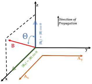
Figure 1: In the Cartesian coordinate system, the magnetic field (B) is oriented in the $x$-$z$ plane at an angle $\Theta$ to the photon’s propagation vector. The transverse component (B_T) aligns with the $x$-axis, parallel to $A_{x}$, while $A_{y}$ is perpendicular to the transverse field.

Assuming the relativistic axion with momentum $k\gg\,m_{\Phi}$, the solution for the field can be expressed as

$$\Phi(z,t)=\Phi(z)e^{-i\omega t}.$$ (7)

We examine a monochromatic light beam propagating along the z-direction. The magnetic field B is located in the $x-z$ plane, illustrated in Figure 1, with $\Theta$ representing the angle between the direction of B and the $z$-axis. Components $A_{x}$ and $A_{y}$ represent the vector potential parallel and perpendicular to $\textbf{B}_{T}$, respectively, where $\textbf{B}_{T}$ denotes the projection of B onto the $x$-axis.

The spatial components of Equation 6, expressed under the Coulomb gauge as:

$$\Box\textbf{A}-\bm{\nabla}\dot{A}^{0}=g_{\Phi\upgamma}\textbf{B}\dot{\Phi}.$$ (8)

The equation governing the behavior of the time component of gauge fields is as follows:

$$\bm{\nabla}^{2}A^{0}=-g_{\Phi\upgamma}\textbf{B}.\bm{\nabla}\Phi.$$ (9)

The dynamics of the axion can be reformulated as follows

$$(\Box-m^{2}_{\Phi})\Phi=-g_{\Phi\upgamma}\textbf{B}.(\dot{\bm{A}}+\bm{\nabla}A^{0}).$$ (10)

From equations 8 and 10, it is evident that only the component of A parallel to B undergoes mixing with the axion. We have made the assumption that B lies in the $x-z$ plane without loss of generality. Now, in the ($x,y,z$) coordinate system, we have the following components for the magnetic field and propagating photons:

$$\textbf{B}=(|\textbf{B}|\sin{\Theta},0,|\textbf{B}|\cos{\Theta}),$$ (11)

$$\textbf{A}=(i\,A_{x}(z),i\,A_{y}(z),0)e^{-i\omega t},$$ (12)

where $\Theta$ is the angle between the direction of B and the $z$-axis. $A_{x}$ and $A_{y}$ represent the components of the photon field along the $x$-axis and $y$-axis, respectively.

For the considered photon-axion system [159, 160, 161, 162, 163] in a constant uniform magnetic field the Lagrangian for the system is [164]

$$\mathcal{L}=\mathcal{L}_{\Phi}+\mathcal{L}_{\Phi\upgamma}+\mathcal{L}_{\upgamma},$$ (13)

here $\mathcal{L}_{\Phi}$ is the axion field Lagrangian defined as

$$\mathcal{L}_{\Phi}=-\frac{1}{2}\bigl{(}\partial_{\mu}\Phi\,\partial^{\mu}\Phi+m_{\Phi}^{2}\Phi^{2}\bigl{)},$$ (14)

The axion-photon interaction $\mathcal{L}_{\Phi\upgamma}$ is

$$\mathcal{L}_{\Phi\upgamma}=-\frac{1}{4}g_{\Phi\upgamma}\Phi\,F_{\mu\nu}\tilde{F}^{\mu\nu}=g_{\Phi\upgamma}\Phi\,\textbf{E.B},$$ (15)

The quantum electrodynamic Lagrangian for photon $\mathcal{L}_{\upgamma}$ is given as

$$\mathcal{L}_{\upgamma}=-\frac{1}{4}\,F_{\mu\nu}F^{\mu\nu}+\mathcal{L}_{EH},$$ (16)

the vacuum polarizability effect arising from photon-photon interaction, in the limit where photon frequencies are considerably smaller than the electron mass and magnetic field strengths are weak in comparison to critical field strengths, is described by the Euler-Heisenberg effective Lagrangian $\mathcal{L}_{EH}$ given as [160]

$$\mathcal{L}_{EH}=\frac{\alpha^{2}}{90\,m_{e}^{4}}\Bigl{[}(F_{\mu\nu}F^{\mu\nu})^{2}+\frac{7}{4}(\tilde{F}_{\mu\nu}F^{\mu\nu})^{2}\Bigr{]},$$ (17)

where $\alpha$ is the fine structure constant (with value $1/137$) and $m_{e}$ is the electron mass ($511$ keV). This Lagrangian emerges from quantum field-theoretic effects, specifically describing one-loop corrections to classical electrodynamics. It contributes the following term on the right-hand side of 6

$$\frac{4\alpha^{2}}{45\,m_{e}^{4}}\partial_{\mu}\Bigl{(}F_{\alpha\beta}F^{\alpha\beta}F^{\mu\nu}+\frac{7}{4}F_{\alpha\beta}\tilde{F}^{\alpha\beta}F^{\mu\nu}\Bigr{)}.$$ (18)

Utilizing Equation (12) and assuming a plane wave solution, we obtain the following equations in the linear order of A

$$F_{\alpha\beta}F^{\alpha\beta} =2|\textbf{B}|^{2}+4\omega|\textbf{B}|\sin{\Theta}A_{y},$$ (19a)

$$F_{\alpha\beta}\tilde{F}^{\alpha\beta} =-4\omega|\textbf{B}|\sin{\Theta}A_{x}.$$ (19b)

The Euler-Heisenberg Lagrangian introduces a modification to Maxwell’s equations through the inclusion of the term

$$\frac{4\alpha^{2}}{45\,m_{e}^{4}}\partial_{\mu}\left[\bigl{(}2|\textbf{B}|^{2}+4\omega|\textbf{B}|\sin{\Theta}A_{y}\bigl{)}\,F^{\mu\nu}+\frac{7}{4}\bigl{(}-4\omega|\textbf{B}|\sin{\Theta}A_{x}\bigl{)}F^{\mu\nu}\right],$$ (20)

With the addition of this term to the right side of equation (8), we get

$$\Box A_{x}+7\omega^{2}\zeta\sin^{2}{\Theta}+\omega g_{\Phi\upgamma}\Phi|\textbf{B}|\sin{\Theta}=0,$$ (21)

$$\Box A_{y}+4\omega^{2}\zeta\sin^{2}{\Theta}A_{y}=0,$$ (22)

where,

$$\zeta=\frac{\alpha}{45\pi}\Bigl{(}\frac{|\textbf{B}|}{|\textbf{B}|_{\text{crit}}}\Bigr{)}^{2}\ \ ,\ \ \ \ \ \ \ |\textbf{B}|_{\text{crit}}=\frac{m_{e}^{2}}{e}.$$ (23)

By introducing a term $-\omega^{2}_{pl}A_{x}$ to the equations of motion, we can account for the influences of the surrounding plasma, with $\omega_{pl}$ is plasma frequency,

$$\omega_{pl}\equiv\sqrt{\frac{4\pi\alpha n_{e}}{m_{e}}}=3.7\times 10^{-11}\text{eV}\sqrt{\frac{n_{e}}{\text{cm}^{-3}}},$$ (24)

where, $n_{e}$ denotes the number density of electrons in the medium through which the photon propagates. Only the $A_{x}$ component undergoes mixing with the axion, leading to the pertinent equations

$$\Box A_{x}-\omega^{2}_{pl}A_{x}+7\omega^{2}\zeta\sin^{2}{\Theta}A_{x}+\omega g_{\Phi\upgamma}\Phi|\textbf{B}|\sin{\Theta}=0,$$ (25)

$$(\Box-m^{2}_{\Phi})\Phi+\omega\,g_{\Phi\upgamma}|\textbf{B}|\sin{\Theta}A_{x}=0.$$ (26)

The solutions of the fields as provided in 4 and 7 can be written as

$$A_{x}(t,z)=\tilde{A}(z)e^{-i(\omega t-kz)}+\text{h.c},$$ (27)

$$\Phi(t,z)=\tilde{\Phi}(z)e^{-i(\omega t-kz)}+\text{h.c}.$$ (28)

The photons, traveling along the z-direction, undergo conversion into axions, and their amplitudes also exhibit variations with the distance $z$. It is expected that these amplitudes change slowly, indicated by the condition that the ratio of the second-order partial derivative to the first-order partial derivative of the amplitudes with respect to the propagation direction $z$ is much less than the momentum $k$ i.e., $|\partial_{z}^{2}\tilde{A}(z)|\ll k|\partial_{z}\tilde{A}(z)|$ and $|\partial_{z}^{2}\tilde{\Phi}(z)|\ll k|\partial_{z}\tilde{\Phi}(z)|$
According to ultra-relativistic limit $|m_{\Phi}^{2}|\gg\omega^{2}$ and $\omega\sim k$ then the operator,

$$\Box =(\omega+i\partial_{z})(\omega-i\partial_{z})=(\omega+i\partial_{z})(\omega+k)$$ (29)

$$\approx 2\omega(\omega+i\partial_{z}).$$

Using this lowest-order approximation, we obtain

$$\Box A_{x}(z,t)\simeq 2i\omega\partial_{z}\tilde{A}(z)e^{-i(\omega t-kz)}+\text{h.c},$$ (30)

$$\Box\Phi(z,t)\simeq 2i\omega\partial_{z}\tilde{\Phi}(z)e^{-i(\omega t-kz)}+\text{h.c}.$$ (31)

The equations of motion simplify to,

$$i\frac{d}{dz}\tilde{A}(z)=\biggl{(}\frac{\omega^{2}_{pl}}{2\omega}-\frac{28\alpha^{2}\omega}{90m^{4}_{e}}\big{(}|\textbf{B}|\sin{\Theta}\big{)}^{2}\biggl{)}\tilde{A}(z)-\frac{1}{2}g_{\Phi\upgamma}|\textbf{B}|\sin{\Theta}\tilde{\Phi}(z),$$ (32)

$$i\frac{d}{dz}\tilde{\Phi}(z)=\biggl{(}-\frac{1}{2}g_{\Phi\upgamma}|\textbf{B}|\sin{\Theta}\biggr{)}\tilde{A}(z)+\frac{m^{2}_{\Phi}}{2\omega}\tilde{\Phi}(z).$$ (33)

Conveniently, we can rewrite the equations as

$$i\frac{d}{dz}\Psi(z)=\textbf{M}\Psi(z),$$ (34)

where,

$$\Psi(z)=\begin{bmatrix}\tilde{A}(z)\\ \tilde{\Phi}(z)\end{bmatrix}\ \ ,\ \ \ \textbf{M}=\begin{bmatrix}\Delta_{\|}&-\Delta_{\text{M}}\\ -\Delta_{\text{M}}&\Delta_{\Phi}\end{bmatrix}$$ (35)

here,

$$\Delta_{\|} =\Delta_{pl}-\Delta_{vac},$$ (36a)

$$\Delta_{pl} \equiv\frac{\omega_{\mathrm{pl}}^{2}}{2\omega}=6.9\times 10^{-25}\mathrm{eV}\left(\frac{n_{e}}{\mathrm{~{}cm}^{-3}}\right)\left(\frac{\mathrm{keV}}{\omega}\right),$$ (36b)

$$\Delta_{vac} \equiv\frac{28\alpha^{2}\omega}{90m_{e}^{4}}(|\mathbf{B}|\sin\Theta)^{2}=9.3\times 10^{-29}\mathrm{eV}\left(\frac{\omega}{\mathrm{keV}}\right)\Bigl{(}\frac{|\mathbf{B}|}{\mathrm{Gauss}}\Bigl{)}^{2}\sin^{2}\Theta,$$ (36c)

$$\Delta_{\mathrm{M}} \equiv\frac{1}{2}g_{\Phi\upgamma}|\mathbf{B}|\sin\Theta=9.8\times 10^{-23}\mathrm{eV}\left(\frac{g_{\Phi\upgamma}}{10^{-11}\mathrm{GeV}^{-1}}\right)\Bigl{(}\frac{|\mathbf{B}|}{\text{ Gauss }}\Bigl{)}\sin\Theta,$$ (36d)

$$\Delta_{\Phi} \equiv\frac{m_{\Phi}^{2}}{2\omega}=5\times 10^{-22}\mathrm{eV}\left(\frac{m_{\Phi}}{\mathrm{neV}}\right)^{2}\left(\frac{\mathrm{keV}}{\omega}\right).$$ (36e)

These $\Delta_{pl}$, $\Delta_{vac}$, $\Delta_{\text{M}}$, $\Delta_{\Phi}$ have been evaluated in our analysis of M$87^{*}$ and are consistently defined as positive, which differs from the definition in [159]. The matrix M exhibits eigenvalues that are

$$\lambda_{\pm}=\frac{(\Delta_{\|}+\Delta_{\Phi})\pm\sqrt{(\Delta_{\|}-\Delta_{\Phi})^{2}+(2\Delta_{\text{M}})^{2}}}{2}$$ (37)

Now we diagonalize M by introducing an orthogonal matrix O such that

$$\textbf{O}^{T}\textbf{M}\textbf{O}=\begin{bmatrix}\lambda_{+}&0\\ 0&\lambda_{-}\end{bmatrix}\ ,\ \ \ \ \textbf{O}\equiv\begin{bmatrix}\cos{v}&\sin{v}\\ -\sin{v}&\cos{v}\end{bmatrix},$$ (38)

where $v$ denotes the mixing angle, given as

$$v=\frac{1}{2}\arctan\left(\frac{2\Delta_{\text{M}}}{\Delta_{\Phi}-\Delta_{\|}}\right).$$ (39)

The Equation 34 becomes,

$$i\frac{d}{dz}(\textbf{O}^{T}\Psi(z))=\begin{bmatrix}\lambda_{+}&0\\ 0&\lambda_{-}\end{bmatrix}(\textbf{O}^{T}\Psi(z)),$$ (40)

Upon solving the equation, we obtain

$$\Psi(z)=\textbf{O}\begin{bmatrix}e^{-iz\lambda_{+}}&0\\ 0&e^{-iz\lambda_{-}}\end{bmatrix}\textbf{O}^{T}\Psi(0)$$ (41)

Ultimately, we have determined the general solutions to be

$$\tilde{A}(z)=\bigr{(}\cos^{2}{v}\,e^{-iz\lambda_{+}}+\sin^{2}{v}\,e^{-iz\lambda_{-}}\bigl{)}\tilde{A}(0)+\sin{v}\cos{v}\bigr{(}e^{-iz\lambda_{+}}-e^{-iz\lambda_{-}}\bigr{)}\tilde{\Phi}(0),$$ (42)

$$\tilde{\Phi}(z)=\sin{v}\cos{v}\bigr{(}e^{-iz\lambda_{+}}-e^{-iz\lambda_{-}}\bigl{)}\tilde{A}(0)+\bigr{(}\cos^{2}{v}\,e^{-iz\lambda_{-}}+\sin^{2}{v}\,e^{-iz\lambda_{+}}\bigr{)}\tilde{\Phi}(0).$$ (43)

With the initial condition $\tilde{\Phi}(0)=0$ and $\tilde{A}(0)=1$, considering the axion density to be negligibly small compared to that of photons, we can determine the probability of photon-to-axion conversion as a function of distance $z$ as

$$P_{\upgamma\rightarrow\Phi}(z) =|\tilde{\Phi}(z)|^{2},$$ (44)

$$=\sin^{2}{2v}\,\sin^{2}{\Bigr{(}\frac{\Delta_{\rm osc}}{2}z\Bigl{)}},$$

$$=\left(\frac{\Delta_{\text{M}}}{\Delta_{\rm osc}/2}\right)^{2}\sin^{2}{\Bigr{(}\frac{\Delta_{\rm osc}}{2}z\Bigl{)}},$$

where, $\Delta_{\rm osc}^{-1}$ represents the oscillation length, defined as

$$\Delta_{\rm osc}\equiv\lambda_{+}-\lambda_{-}=\sqrt{(\Delta_{\Phi}-\Delta_{\|})^{2}+(2\Delta_{\text{M}})^{2}}.$$ (45)

The conversion of photons to axions crucially depends on determining $\Delta_{\text{M}}$ using the parameters $g_{\Phi\upgamma}$ and $|\textbf{B}_{T}|$. The conversion process is hindered by the contributions of finite axion mass encoded in $\Delta_{\Phi}$, one-loop corrections of electrons encoded in $\Delta_{vac}$, and plasma contribution encoded in $\Delta_{pl}$. In the case of relativistic axions, the frequency of the propagating photons, i.e, $\omega$ is markedly greater than the axion mass $m_{\Phi}$, and for photons traversing through a medium, $\omega$ significantly exceeds the plasma frequency $\omega_{pl}$. To confirm the validity of the current framework, a minimum of three of the following requirements must be fulfilled:

1. $$\frac{\alpha}{45\pi}\left(\frac{|\mathbf{B}|}{|\mathbf{B}|_{\text{crit}}}\right)^{2}\ll 1,$$

   $$\text{where }|\mathbf{B}|_{\text{crit}}\equiv\frac{m_{e}^{2}}{\sqrt{4\pi\alpha}}=4\times 10^{13}\ \text{Gauss},$$

   where $m_{e}$ is the mass of the elctron and $\alpha$ is the structure constant.

2. To validate the assumption of relativistic axions, it is necessary that

   $$\omega\gg m_{\Phi},$$

3. For photons to move effectively in the surrounding plasma, it is essential that

   $$\omega\gg\omega_{pl}.$$

From 44 and 45, one can notice that the condition for the most effective conversion probability is

$$\left(\Delta_{\Phi}+\Delta_{\rm vac}-\Delta_{\rm pl}\right)^{2}\ll 4\Delta_{M}^{2}$$ (46)

For such scenario, using 45, one can find the characteristic length scale associated with the most effective conversion as

$$\Delta_{\rm osc}^{-1}\simeq\left(2\Delta_{M}\right)^{-1}=3.4\times 10^{2}\times\left(2\times 10^{9}M_{\odot}\right)\times\left(\dfrac{\text{Gauss}}{|\mathbf{B}|}\right)\left(\dfrac{10^{-11}\rm Gev^{-1}}{g_{\Phi\upgamma}}\right)$$ (47)

For supermassive compact object M$87^{*}$, the mass has been reported to be $6.2^{+1.1}_{-0.5}\times 10^{9}~{}M_{\odot}$ along with the associated magnetic field in the vicinity of the compact object to be around $(1-30)$ Gauss. Again from 47, one can notice that for the magnetic field $|\mathbf{B}|\sim 10^{1-2}$ Gauss, the conversion length becomes comparable to Schwarzschild radius of a supermassive black hole of mass around $10^{9}~{}M_{\odot}$ if the coupling constant is $g_{\Phi\upgamma}\sim 10^{-11}~{}\rm GeV^{-1}$. So, for supermassive compact object M$87^{*}$, we can expect the conversion to axion to occur efficiently since photons can stay at the photon sphere for a considerable amount of time.

3 Geodesic motion of photons

We consider the geodesic motion of photon in a static spacetime with spherical symmetry. In this case, the magnetic field strength is on the order of Gauss, and it is not strong enough to have any appreciable back reaction on the spherically symmetric geometry. The general spherically symmetric metric is given by

$$ds^{2}=-f(r)dt^{2}+\dfrac{1}{g(r)}dr^{2}+r^{2}\mathcal{R}^{2}(r)\left(d\theta^{2}+\sin^{2}\theta d\phi^{2}\right)$$ (48)

If $\lambda$ is treated as affine parameter, then the geodesic of a photon can be represented by $x^{\alpha}(\lambda)=\{t(\lambda),r(\lambda),\theta(\lambda),\phi(\lambda)\}$. the spherical symmetry of spacetime ensures the existence of two Killing vectors: $t^{\mu}=(1,0,0,0)$ and $\phi^{\mu}=(0,0,0,1)$. Also, without loss of generality, we can assume the geodesic of the photon to be at $\theta=\pi/2$. Due to the existence of these Killing vectors, we can introduce two conserved quantities as

$$E =f(r)\dfrac{dt}{d\lambda}$$ (49a)

$$L =r^{2}\mathcal{R}^{2}(r)\dfrac{d\phi}{d\lambda}$$ (49b)

One can interpret the conserved quantities $E$ and $L$ as the energy and the angular momentum of the orbiting photon.

Now if $s$ is a dimensionful parameter, then the four momentum of the photon can be given by $p^{\mu}=E\dfrac{dx^{\mu}}{ds}$. With such definition, the null geodesic satisfies the following equations:

$$\dfrac{dr}{ds} =\pm\sqrt{\mathbb{R}(r)},\hskip 28.45274pt\mathbb{R}(r)=\mathcal{A}(r)(1-V_{\rm eff})$$ (50a)

$$\dfrac{d\phi}{ds} =\dfrac{b}{r^{2}\mathcal{R}^{2}(r)}$$ (50b)

$$\dfrac{dt}{ds} =-\dfrac{1}{f(r)}$$ (50c)

where, we have used the following definitions:

$$\mathcal{A}(r) =\dfrac{g(r)}{f(r)}$$ (51a)

$$V_{\rm eff} =\dfrac{b^{2}}{r^{2}\mathcal{R}^{2}(r)}f(r)$$ (51b)

The radius at which photons have zero radial velocity and can circle a central gravitational object at a fixed radial distance is known as the photon sphere. To determine the radius of the photon sphere, we need to employ the following conditions: $\mathbb{R}(r)=0$ and $\dfrac{\differential\mathbb{R}}{\differential r}=0$. Let us assume the radius of the photon sphere is $r_{ph}$. This can be determined with the help of the following equation

$$\dfrac{f^{\prime}(r_{ph})}{f(r_{ph})}=2\left[\dfrac{1}{r_{ph}}+\dfrac{\mathcal{R}^{\prime}(r_{ph})}{\mathcal{R}(r_{ph})}\right]$$ (52)

At the photon sphere, the critical impact parameter for photons with zero radial velocity is provided by

$$b_{c}=\dfrac{r_{ph}\mathcal{R}(r_{ph})}{\sqrt{f(r_{ph})}}$$ (53)

We will now examine the behaviour of photon geodesics in a perturbative approach close to the photon sphere[165]. Here are the definitions of dimensionless fractional variations of the radius and the critical impact parameter around the photon sphere

$$r =r_{ph}(1+\delta r)$$ (54a)

$$b =b_{c}(1+\delta b)$$ (54b)

One can obtain the critical value of the impact parameter by expanding it as follows

$$\dfrac{b}{b_{c}} =1+\bigg{[}\dfrac{1}{8}\left\{\dfrac{4r_{ph}f^{\prime}(r_{ph})}{f(r_{ph})}+\left(\dfrac{r_{ph}f^{\prime}(r_{ph})}{f(r_{ph})}\right)^{2}-2r_{ph}^{2}\left(\dfrac{f^{\prime\prime}(r_{ph})}{f(r_{ph})}-\dfrac{2\mathcal{R}^{\prime\prime}(r_{ph})}{\mathcal{R}(r_{ph})}\right)\right\}-1\bigg{]}\delta r^{2}+\mathcal{O}\left(\delta r^{3}\right)$$ (55)

As we are interested in the orbits that are close to the photon sphere, $\delta r$ and $\delta b$ must be taken simultaneously to zero at a rate $\delta b\propto\delta r^{2}$. With the leading term retained, this approximation provides the form of $\mathbb{R}(r)$ around the photon sphere as

$$\mathbb{R}(r)=\mathcal{A}(r_{ph})\left(\mathcal{P}\delta r^{2}-2\delta b\right)$$ (56)

where we have defined

$$\mathcal{P}\equiv 1+r_{ph}^{2}\left[\left\{\dfrac{f^{\prime}(r_{ph})}{f(r_{ph})}\right\}^{2}-3\left\{\dfrac{\mathcal{R}^{\prime}(r_{ph})}{\mathcal{R}(r_{ph})}\right\}^{2}-\dfrac{2f^{\prime}(r_{ph})}{r_{ph}f(r_{ph})}-\dfrac{f^{\prime\prime}(r_{ph})}{2f(r_{ph})}+\dfrac{\mathcal{R}^{\prime\prime}(r_{ph})}{\mathcal{R}(r_{ph})}\right]$$ (57)

and

$$\bigg{[}\dfrac{1}{8}\left\{\dfrac{4r_{ph}f^{\prime}(r_{ph})}{f(r_{ph})}+\left(\dfrac{r_{ph}f^{\prime}(r_{ph})}{f(r_{ph})}\right)^{2}-2r_{ph}^{2}\left(\dfrac{f^{\prime\prime}(r_{ph})}{f(r_{ph})}-\dfrac{2\mathcal{R}^{\prime\prime}(r_{ph})}{\mathcal{R}(r_{ph})}\right)\right\}-1\bigg{]}\left(\dfrac{M}{r_{ph}}\right)^{2}\equiv\mathfrak{a}$$ (58)

Setting the potential to zero yields the turning point. In the vicinity of the photon sphere, using the leading order approximation, we have

$$\delta r_{turn}=\sqrt{\dfrac{2\delta b}{\mathcal{P}}}$$ (59)

We need to find the amount of affine parameter in the region $-\updelta R<\delta r<\updelta R$ around the photon sphere, such that $0<\updelta R\ll 1$. From 56, we can conclude that there is no turning point for $\delta b<0$. In this particular case, we have

$$\Delta s=\int_{-\updelta R}^{\updelta R}\dfrac{r_{ph}\differential\delta r}{\sqrt{\mathcal{A}(r_{ph})}\sqrt{\mathcal{P}\delta r^{2}-2\delta b}}=\dfrac{r_{ph}}{\sqrt{\mathcal{A}(r_{ph})}}\dfrac{1}{\sqrt{\mathcal{P}}}\ln\left[\dfrac{\mathcal{P}\updelta R^{2}}{-2\delta b}\left(1+\sqrt{1-\dfrac{2\delta b}{\mathcal{P}\updelta R^{2}}}\right)\right]$$ (60)

Using 60, One can notice the existence of logarithmic divergence when $\delta b$ is approached to zero. One can also notice that we can have a single turning point if we consider the case $\delta b>0$. For this case, we need to consider $\updelta R>\delta r_{\rm turn}$ for photons to graze the region of our interest. In particular, for $\delta>0$, we can calculate the change in the affine parameter as

$$\Delta s=2\times\dfrac{r_{ph}}{\sqrt{\mathcal{A}(r_{ph})}}\int_{\sqrt{\frac{2}{\mathcal{P}}\delta b}}^{\updelta R}\dfrac{\differential\delta r}{\sqrt{\mathcal{P}\delta r^{2}-2\delta b}}=\dfrac{r_{ph}}{\sqrt{\mathcal{P}\mathcal{A}(r_{ph})}}\ln\left[\dfrac{\mathcal{P}\updelta R^{2}}{2|\delta b|}\left(1+\sqrt{1-\dfrac{2\delta b}{\mathcal{P}\updelta R^{2}}}\right)^{2}\right]\Theta\left(\updelta R^{2}-\dfrac{2}{\mathcal{P}}\delta b\right)$$ (61)

Further, considering $\delta b\ll\frac{\mathcal{P}}{2}\updelta R^{2}$, we have

$$\Delta s\approx\dfrac{r_{ph}}{\sqrt{\mathcal{P}\mathcal{A}(r_{ph})}}\ln\left[2\mathcal{P}\dfrac{\updelta R^{2}}{\delta b}\right]$$ (62)

Now using 62 and 50, we can have the lapse in time $t$ near the photon sphere as

$$\Delta t\simeq-\dfrac{1}{f(r_{ph})}\dfrac{r_{ph}}{\sqrt{\mathcal{P}}\sqrt{\mathcal{A}(r_{ph})}}\ln\left[\dfrac{2(b-b_{c})}{\mathcal{P}b_{c}}\times\dfrac{r_{ph}^{2}}{\epsilon^{2}M^{2}}\right]\equiv\mathfrak{T}(b)$$ (63)

where the small parameter has been redefined as

$$\epsilon=\left(\dfrac{r_{ph}}{M}\right)\delta r$$ (64)

Here $M$ is the mass parameter of the given spacetime.

4 Photons approaching the photon sphere

4.1 Connection between impact parameter and emission angle

Let us consider a beam of light directed towards the photon sphere of a compact object with an impact parameter $b$ from a point $p_{e}$ located at $r_{e}$ in spherically symmetric spacetime coordinates. Introducing an angle $\Upsilon_{e}$ between the initial direction of the incident photon and the line toward the centre of the compact object, as shown in 2, allows us to characterize the trajectory of the photon.

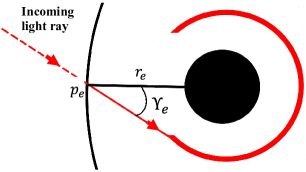
Figure 2: The trajectory of the light ray originating from a point $p_{e}$ towards the photon sphere is depicted by the red curve. This point, $p_{e}$, is situated on a sphere with a radius denoted as $r_{e}$, centred around the compact object within a spherically symmetric coordinate system. The angle $\Upsilon_{e}$ corresponds to the zenith angle.

In the context of the spherically symmetric spacetime described by the 48 and assuming $g(r)=f(r)$, the tetrad vectors are provided by

$$e^{(0)}=\left(\sqrt{f(r)},0,0,0\right),$$ (65a)

$$e^{(1)}=\left(0,\frac{1}{\sqrt{f(r)}},0,0\right),$$ (65b)

$$e^{(2)}=\left(0,0,r\mathcal{R}(r),0\right),$$ (65c)

$$e^{(3)}=\left(0,0,0,r\mathcal{R}(r)\sin\theta\right).$$ (65d)

The tetrads $e^{(1)}$ and $e^{(3)}$ serve as orthonormal bases, aligning parallel and perpendicular to the path leading to the centre of compact objects, respectively. Consequently, the angle $\Upsilon_{e}$ is expressed as:

$$\tan\Upsilon_{e}=\left|\frac{k^{\mu}e_{\mu}^{(3)}}{k^{\mu}e_{\mu}^{(1)}}\right|_{p_{e}}=\left|r\mathcal{R}(r)\sqrt{f(r)}\sin\theta\frac{d\phi}{dr}\right|_{p_{e}},$$ (66)

here, $k^{\mu}={dx^{\mu}}/{d\lambda}$ represents the tangent vector tracing the geodesics of the photons with the affine parameter $\lambda$. For simplicity, we assume that the geodesic plane lies in the $\theta=\pi/2$ plane. Using 50, we derive

$$b=\frac{r_{e}\mathcal{R}(r_{e})}{\sqrt{f\left(r_{e}\right)}}\sin\Upsilon_{e}.$$ (67)

This equation establishes a link between the emission angle $\Upsilon_{e}$, evaluated at $p_{e}$, and the impact parameter $b$.

4.2 Photon sphere inflow from spherical region

We envision the compact object situated at the centre of a sphere, where photons are emitted isotropically from every point with a specific emissivity. We aim to estimate the approximate number of photons approaching a photon sphere. To accomplish this, we adopt a spherically symmetric spacetime as our model geometry.

Let $\differential N/\differential\tau_{e}$ represent the number of photons emitted with a frequency width $d\omega_{e}$ from $dV_{e}$, and travelling through an infinitesimal solid angle $d\omega_{e}$ per unit time $\tau_{e}$ as observed from the emission point $p_{e}$. Here, $V_{e}$, $\omega_{e}$, $\tau_{e}$, and $\Omega$ are all in a local inertial frame at $p_{e}$, as shown in 3.

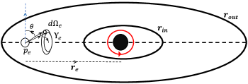
Figure 3: Photons are emitted from a spherical region with boundaries defined by $r_{in}$ and $r_{out}$, and they converge towards the photon sphere of the compact object, which is represented by the red circle.

Designating $\Psi_{e}$ as the azimuthal angle in the plane perpendicular to the direction from point $p_{e}$ to the compact object, and $\Upsilon_{e}$ as the zenithal angle measured from that direction, we assume isotropic emission from $p_{e}$. Under this assumption, we consider $J_{e}$ to be independent of $\Upsilon_{e}$ and $\Psi_{e}$. Hence, the expression for a photon with all the conditions is given as

$$\differential^{6}\left(\frac{\differential N}{\differential\tau_{e}}\right)=J_{e}\left(\omega_{e},r_{e}\right)\differential\Omega_{e}\differential V_{e}\differential\omega_{e}.$$ (68)

We reframe 68 in relation to the impact parameter $b$ of a photon. Employing 67 and $\differential b=(r_{e}\mathcal{R}(r_{e})/\sqrt{f(r_{e})})\cos{\Upsilon_{e}}d\Upsilon_{e}$, we obtain the intended outcome for a constant $r_{e}$. Upon integration 68 across the angle $\Psi_{e}$, we determine the number of photons emitted towards the direction of the photon sphere per unit time as

$$\differential^{5}\left(\frac{\differential N}{\differential\tau_{e}}\right)=\frac{1}{2}\times 2\pi J_{e}\left(\omega_{e},r_{e}\right)\dfrac{\sqrt{f\left(r_{e}\right)}}{r_{e}\mathcal{R}(r_{e})}\dfrac{b}{\sqrt{\dfrac{r_{e}^{2}\mathcal{R}^{2}(r_{e})}{f\left(r_{e}\right)}-b^{2}}}\times\differential b\,\differential V_{e}\differential\omega_{e}$$ (69)

To account for the restriction that only photons within angle of $0\leq\Upsilon\leq\pi/2$ can approach the photon sphere, we multiply by a factor of $1/2$ in 69. Within a local inertial frame at $p_{e}$, with volume element $\differential V_{e}=(r_{e}^{2}\mathcal{R}^{2}(r_{e})/\sqrt{f(r_{e})})\sin{\theta}\differential r_{e}\,\differential\theta\differential\phi$ and the time element $\differential\tau_{e}=\sqrt{f(r_{e})}\differential t$ in spherically symmetric spacetime, the number count of photons with an impact parameter falling within the range $(b,b+\differential b)$, emanating from a spherical shell with a width of $\differential r_{e}$ and a unit frequency of $\omega_{e}$, is determined by integrating 69 over $\theta$ and $\phi$, given as

$$\frac{\differential^{4}N}{\differential t\differential\omega_{e}\differential b\differential r_{e}}=4\pi^{2}J_{e}\left(\omega_{e},r_{e}\right)\frac{br_{e}\mathcal{R}(r_{e})\sqrt{f\left(r_{e}\right)}}{\sqrt{\dfrac{r_{e}^{2}\mathcal{R}^{2}(r_{e})}{f\left(r_{e}\right)}-b^{2}}}.$$ (70)

It is important to note that $\omega_{e}$ represents the frequency in a local inertial frame at the emission point $p_{e}$, and it is defined as

$$\omega_{e}=\left.k^{\mu}e_{\mu}^{(0)}\right|_{p_{e}}=\left.\frac{dt}{d\lambda}\sqrt{f\left(r_{e}\right)}\right|_{p_{e}}=\frac{E}{\sqrt{f\left(r_{e}\right)}},$$ (71)

here, $k^{\mu}=\differential x^{\mu}/\differential\lambda$ represents the tangent vector to the geodesic, $\lambda$ denotes the affine parameter, and $e^{(\alpha)}_{\mu}$ signifies the local tetrad at the emission point $p_{e}$. The frequency measured in a local inertial frame at the photon sphere situated at $r=r_{{ph}}$ is denoted as $\omega_{c}\equiv\dfrac{E}{\sqrt{f(r_{ph})}}$. With an impact parameter in the range $(b,b+db)$, the quantity of photons that reach the photon sphere within a specific time interval $dt$ and frequency $\omega_{c}$ is governed by

$$\left(\frac{\differential^{3}N}{\differential t\differential\omega_{c}\differential b}\right)=4\pi^{2}\int_{r_{\text{in }}}^{r_{\text{out }}}\mathrm{d}r_{e}J_{e}\left(\frac{\sqrt{f\left(r_{{ph}}\right)}\omega_{c}}{\sqrt{f\left(r_{e}\right)}},r_{e}\right)\times\dfrac{br_{e}\mathcal{R}(r_{e})\sqrt{f\left(r_{e}\right)}}{\sqrt{\dfrac{r_{e}^{2}\mathcal{R}^{2}(r_{e})}{f\left(r_{e}\right)}-b^{2}}}.$$ (72)

In this context, the emission region is confined within a spherical region with an inner radius $r_{\mathrm{in}}$ and an outer radius $r_{\mathrm{out}}$. Given our focus on the vicinity of the photon sphere, integrating 72 within the range ($b_{c},b_{c}(1+\mathfrak{a}\epsilon^{2})$), we obtain

$$\frac{\differential^{2}N}{\differential t\differential\omega_{c}}\simeq 4\pi^{2}\mathfrak{a}\epsilon^{2}b_{c}^{2}\int_{r_{\text{in }}}^{r_{\text{out }}}\mathrm{d}r_{e}J_{e}\left(\frac{\sqrt{f\left(r_{\mathrm{ph}}\right)}\omega_{c}}{\sqrt{f\left(r_{e}\right)}},r_{e}\right)\times\frac{r_{e}\mathcal{R}(r_{e})\sqrt{f\left(r_{e}\right)}}{\sqrt{\dfrac{r_{e}^{2}\mathcal{R}^{2}(r_{e})}{f\left(r_{e}\right)}-b_{c}^{2}}},$$ (73)

Here, it is presumed that $r_{e}$ is significantly greater than the radius of the photon sphere, such that $r_{\text{in}}^{2}\mathcal{R}^{2}(r_{\rm in})/f(r_{\text{in}})>b^{2}$ holds for $b$ in the range ($b_{c},b_{c}(1+\mathfrak{a}\epsilon^{2})$).

4.3 Photonic sources in the proximity to galactic compact objects

Recent observations have revealed the presence of an electromagnetic plasma in the vicinity of a supermassive compact object [72]. Photons with frequencies significantly higher than the plasma frequency ($\omega\gg\omega_{pl}$) can traverse this plasma. This high-frequency radiation originates from charged particles being accelerated within the Coulomb field of another charge, a phenomenon commonly referred to as free-free emission or bremsstrahlung. Understanding this process thoroughly requires a quantum treatment, as it enables the production of photons with energies comparable to those of the emitting particles. The energy emitted by this process per unit time, per unit frequency, and unit volume is mathematically represented as [166]

$$\frac{\differential W}{\differential\tau_{e}\differential\omega_{e}\differential V_{e}}=\frac{2^{4}\alpha^{3}}{3m_{e}}\left(\frac{2\pi}{3m_{e}}\right)^{1/2}T_{e}^{-1/2}n_{e}^{2}e^{-\omega_{e}/T_{e}}\bar{g}_{ff},$$ (74)

here, $T_{e}$ represents the electron temperature, $n_{e}$ denotes the electron number density in the plasma, and $\bar{g}_{ff}$ represents the velocity-averaged Gaunt factor for free emission. The emission rate is expressed as an approximate classical result multiplied by the free emission Gaunt factor $\bar{g}_{ff}$, which takes into account the quantum-mechanical Born approximation. Although $\bar{g}_{ff}$ is a function of the energy of the electron and the frequency of emission, for order-of-magnitude estimation, can be considered to be approximately unity. Additionally, we assume that the ion density $n_{i}$ is equal to $n_{e}$. For isotropic radiation, $J_{e}^{(N)}$ as defined in 68 gives

$$J_{e}^{(N)}\left(\omega_{e},r_{e}\right)=\frac{1}{4\pi\omega_{e}}\left(\frac{2^{4}\alpha^{3}}{3m_{e}}\right)\left(\frac{2\pi}{3m_{e}}\right)^{1/2}\times T_{e}^{-1/2}n_{e}^{2}e^{-\omega_{e}/T_{e}}\bar{g}_{ff}.$$ (75)

The Event Horizon Telescope (EHT) images of M87* reveal a bright ring-like structure, corresponding to the emission from the inner part of the hot accretion disk. The observed properties of the emission, such as its spectrum and variability, align with expectations from a hot accretion flow. The temperature of hot accretion is nearly virial, approximately $T\approx GMm_{p}/6k_{B}r\approx 10^{12}K(r/M)^{-1}$, with $m_{p}$ representing the proton mass [167, 168]. When studying accretion processes around supermassive compact objects like M87*, theoretical models are commonly employed to understand the properties and behaviour of the accreting material. One such model is the spherical accretion model, which assumes that the accretion flow onto the compact object is spherically symmetric. However, it’s important to note that while the spherical accretion model serves as a useful starting point for understanding the overall behaviour of the accretion flow around M87*, it simplifies the actual complex processes that may occur. The spherical mass accretion rate can be expressed as $M=4\pi r^{2}\rho v_{r}$, with mass density $\rho$ and radial velocity $v_{r}$. Assuming constant mass accretion and free-falling gas, $vr\alpha r^{-1/2}$, we find that $\rho\alpha(r/M)^{-3/2}$. Consequently, we can assume that the electron temperature and number density of electrons obey a power law

$$T_{e}=T_{e,c}\left(\frac{r_{e}}{r_{\mathrm{ph}}}\right)^{-1},$$ (76a)

$$n_{e}=n_{e,c}\left(\frac{r_{e}}{r_{\mathrm{ph}}}\right)^{-3/2},$$ (76b)

where $T_{e,c}$ and $n_{e,c}$ denote the value at the photon sphere.

5 Relative luminosity and conversion of photons into axions

5.1 Relationship between the spacetime metric and the conversion probability and factor

In the preceding section, we explored the presence of the photon sphere within a generally spherically symmetric spacetime and calculated the photon time-lapse in such contexts. To streamline our analysis, we adopt the universal spherically symmetric metric in the following form:

$$ds^{2}=-f(r)dt^{2}+\dfrac{1}{f(r)}dr^{2}+r^{2}\mathcal{R}^{2}(r)\left(d\theta^{2}+\sin^{2}\theta d\phi^{2}\right)$$ (77)

The period during which photons remain near the photon sphere and their impact parameter $b$ is close to critical value $b_{c}$ around the photon sphere ($r_{ph}<r<r_{ph}(1+\delta r)$) is given by

$$\mathfrak{T}(b)=-\dfrac{1}{f(r_{ph})}\dfrac{r_{ph}}{\sqrt{\mathcal{P}}}\ln\left[\dfrac{2(b-b_{c})}{\mathcal{P}b_{c}}\dfrac{r_{ph}^{2}}{\epsilon^{2}M^{2}}\right]$$ (78)

The following equation can be used to determine how many photons near the photon sphere converted to axions per unit time $t$ and unit frequency $\omega_{c}$,

$$\dfrac{\differential^{2}N_{\upgamma\to\Phi}}{\differential t\differential\omega_{c}}=\int_{b_{c}}^{b_{c}(1+\mathfrak{a}\epsilon^{2})}\differential b\dfrac{1}{2}\left(\dfrac{\differential^{3}N}{\differential t\differential\omega_{c}\differential b}\right)P_{\upgamma\to\Phi}\left(\sqrt{f(r_{ph})}\mathfrak{T}(b)\right)$$ (79)

where

$$P_{\upgamma\to\Phi}\left(\sqrt{f(r_{ph})}\mathfrak{T}(b)\right)=\left(\dfrac{2\Delta_{M}}{\Delta_{\rm osc}}\right)^{2}\times\sin^{2}\left(-\dfrac{\Delta_{\rm osc}}{2}\dfrac{1}{\sqrt{f(r_{ph})}}\dfrac{r_{ph}}{\sqrt{\mathcal{P}}}\ln\left[\dfrac{2(b-b_{c})}{\mathcal{P}b_{c}}\dfrac{r_{ph}^{2}}{\epsilon^{2}M^{2}}\right]\right)$$ (80)

The factor of $1/2$ in 79 represents the proportionality between photons with polarisation parallel to the external magnetic field and the production of axions. The number of photons entering the region $r_{ph}<r<r_{ph}\left(1+\epsilon M/r_{ph}\right)$ and escaping to infinity can be found by integrating over the interval $(b_{c},,b_{c}(1+\mathfrak{a}\epsilon^{2}))$. Since there is no significant variation in the number of photons when the impact parameter changes in this situation, we can approximate it by considering its value at $b=b_{c}$ outside the integral. Then 79 takes the following form

$$\dfrac{\differential^{2}N_{\upgamma\to\Phi}}{\differential t\differential\omega_{c}}\simeq\dfrac{1}{2}\left(\dfrac{\differential^{3}N}{\differential t\differential\omega_{c}\differential b}\right)\bigg{|}_{b}\times\left(\dfrac{2\Delta_{\rm M}}{\Delta_{\rm osc}}\right)^{2}\int_{b_{c}}^{b_{c}(1+\mathfrak{a}\epsilon^{2})}\sin^{2}\left[\dfrac{\Delta_{\rm osc}}{2}\mathfrak{T}(b)\sqrt{f(r_{ph})}\right]\differential b$$ (81)

The integral in 81 can further be simplified as

$$\mathcal{I}=\int_{b_{c}}^{b_{c}(1+\mathfrak{a}\epsilon^{2})}\differential b~{}\sin^{2}\left[\dfrac{\Delta_{\rm osc}}{2}\mathfrak{T}(b)\sqrt{f(r_{ph})}\right]=\dfrac{1}{2}\left(\dfrac{1}{1+\mathcal{Y}^{2}}\right)\mathfrak{a}b_{c}\epsilon^{2}$$ (82)

where we have used the following definition

$$\mathcal{Y}=\dfrac{\sqrt{\mathcal{P}}\sqrt{f(r_{ph})}}{r_{ph}\Delta_{\rm osc}}$$ (83)

The fraction of photons that transform into axions when entering the vicinity of the photon sphere is provided as

$$\frac{\differential^{2}N_{\upgamma\rightarrow\phi}}{\differential t\differential\omega_{c}}\bigg{/}\dfrac{\differential^{2}N}{\differential t\differential\omega_{c}}\simeq\dfrac{1}{4}\left(\frac{2\Delta_{\rm M}}{\Delta_{\rm osc}}\right)^{2}\left(\dfrac{1}{1+\mathcal{Y}^{2}}\right)$$ (84)

Now, in the scenario of efficient conversion, we can choose the condition to be $\Delta_{\rm osc}\simeq 2\Delta_{\rm M}$. In this particular case, the conversion factor(C.F.) can be given by

$$CF=\frac{\differential N_{\upgamma\rightarrow\Phi}}{\differential t\differential\omega_{c}}\bigg{/}\dfrac{\differential^{2}N}{\differential t\differential\omega_{c}}\Bigg{|}_{\text{ efficient conversion}} \simeq\dfrac{1}{4}\left(\dfrac{1}{1+\mathcal{Y}^{2}}\right)$$ (85)

$$=\dfrac{1}{4}\left[\dfrac{\left(\dfrac{r_{ph}}{M}\right)^{2}\left(2M\Delta_{\rm M}\right)^{2}}{\left(\dfrac{r_{ph}}{M}\right)^{2}\left(2M\Delta_{\rm M}\right)^{2}+{\mathcal{P}f(r_{ph})}}\right]$$ (86)

Now, inserting 73 into the 81, we have

$$\dfrac{\differential^{2}N_{\upgamma\to\Phi}}{\differential t\differential\omega_{c}} \simeq{\mathfrak{a}\pi^{2}\epsilon^{2}}b_{c}\left(\dfrac{2\Delta_{\rm M}}{\Delta_{\rm osc}}\right)^{2}\left[\dfrac{\left(\Delta_{\rm osc}r_{ph}\right)^{2}}{\left(\Delta_{\rm osc}r_{ph}\right)^{2}+\mathcal{P}f(r_{ph})}\right]$$

$$\hskip 113.81102pt\times\int_{r_{\rm in}}^{r_{\rm out}}\differential r_{e}J_{e}\left(\frac{\sqrt{f(r_{ph})}\omega_{c}}{\sqrt{f(r_{e})}},r_{e}\right)\left[\frac{br_{e}\mathcal{R}(r_{e})\sqrt{f(r_{e})}}{\sqrt{\dfrac{r_{e}^{2}\mathcal{R}^{2}(r_{e})}{f(r_{e})}-b^{2}}}\right]$$ (87)

5.1 helps us to determine the number of axions produced during the conversion of photons into axion.

5.2 Scattering of photons by the plasma

In earlier analysis, for the shake of simplicity, we have neglected the possibility of the scattering of photons by the surrounding plasma while it propagate through the plasma. While taking into consideration the fact that photons have a limited mean free path while incorporating the scattering phenomena, the expression for the number of photons that are converted into axions per unit time and unit frequency as given in 79 needs to be modified in the following way

$$\dfrac{\differential^{2}N_{\upgamma\to\Phi}}{\differential t\differential\omega}=\int_{b_{c}}^{b_{c}(1+\mathfrak{a}\epsilon^{2})}\differential b\dfrac{1}{2}\left(\dfrac{\differential^{3}}{\differential t\differential\omega_{c}\differential b}\right)P_{\upgamma\to\Phi}\left(\sqrt{f(r_{ph})}\mathfrak{T}(b)\right)\exp\left(-\dfrac{\sqrt{f(r_{ph})}\mathfrak{T}(b)}{\ell}\right)$$ (88)

where $\ell$ denotes the mean free path of the propagating photons. Implementing similar treatment like 81, one can come up with the following equation

$$\dfrac{\differential^{2}N_{\upgamma\to\Phi}}{\differential t\differential\omega}=\dfrac{1}{2}\left(\dfrac{\differential^{3}N}{\differential t\differential\omega_{c}\differential t}\right)\bigg{|}_{b=b_{c}}\times\left(\dfrac{2\Delta_{M}}{\Delta_{\rm osc}}\right)^{2}\times\int_{b_{c}}^{b_{c}(1+\mathfrak{a}\epsilon^{2})}\differential b\sin^{2}\left[\dfrac{\Delta_{\rm osc}}{2}\mathfrak{T}(b)\sqrt{f(r_{ph})}\right]\exp\left(-\dfrac{\sqrt{f(r_{ph})}\mathfrak{T}(b)}{\ell}\right)$$ (89)

Let us define the quantity

$$\mathcal{Z}\equiv\dfrac{1}{\ell\Delta_{\rm osc}}$$ (90)

The integral in 89 can be simplified as

$$\widetilde{\mathcal{I}} =\int_{b_{c}}^{b_{c}(1+\mathfrak{a}\epsilon^{2})}\differential b\sin^{2}\left[\dfrac{\Delta_{\rm osc}}{2}\mathfrak{T}(b)\sqrt{f(r_{ph})}\right]\exp\left(-\dfrac{\sqrt{f(r_{ph})}\mathfrak{T}(b)}{\ell}\right)$$ (91)

$$=\dfrac{\mathfrak{a}b_{c}\epsilon^{2}\mathcal{Y}}{2}\int_{0}^{\infty}\differential x~{}~{}(1-\cos x)\exp\left\{-(\mathcal{Z+Y})x\right\}$$

$$=\dfrac{1}{2}\mathfrak{a}b_{c}\epsilon^{2}\dfrac{1}{\left(1+\dfrac{\mathcal{Z}}{\mathcal{{Y}}}\right)\left\{1+(\mathcal{Y+Z})^{2}\right\}}$$ (92)

Hence the number of photons converted into axions per unit time per unit frequency is provided by

$$\dfrac{\differential^{2}N_{\upgamma\to\Phi}}{\differential t\differential\omega} =\dfrac{\mathfrak{a}b_{c}\epsilon^{2}}{4}\left(\dfrac{\differential^{3}N}{\differential t\differential\omega_{c}\differential t}\right)\bigg{|}_{b=b_{c}}\left(\dfrac{2\Delta_{M}}{\Delta_{\rm osc}}\right)^{2}\left[\left(1+\dfrac{\mathcal{Z}}{\mathcal{Y}}\right)\left\{1+(\mathcal{Y+Z})^{2}\right\}\right]^{-1}$$ (93)

$$=\dfrac{\mathfrak{a}b_{c}\epsilon^{2}}{4}\left(\dfrac{\differential^{3}N}{\differential t\differential\omega_{c}\differential t}\right)\bigg{|}_{b=b_{c}}\left(\dfrac{2\Delta_{M}}{\Delta_{\rm osc}}\right)^{2}\left[\left(1+\dfrac{1}{\left(\dfrac{\ell}{r_{ph}}\right)\sqrt{\mathcal{P}}\sqrt{f(r_{ph})}}\right)\left\{1+\left(\dfrac{1+\left(\dfrac{\ell}{r_{ph}}\right)\sqrt{\mathcal{P}}\sqrt{f(r_{ph})}}{\left(\dfrac{\ell}{r_{ph}}\right)~{}\left(\dfrac{r_{ph}}{M}\right)M\Delta_{\rm osc}}\right)^{2}\right\}\right]^{-1}$$ (94)

It is important to note that we can retrieve 86 with help of 94 when the following condition holds

$$\dfrac{\ell/M}{\dfrac{1}{\sqrt{\mathcal{P}}\sqrt{f(r_{ph})}}\left(\dfrac{r_{ph}}{M}\right)}\ggg 1$$ (95)

The mean free path for photons with a frequency lower than the electron mass $m_{e}$ is provided by

$$\dfrac{\ell}{M}=\dfrac{1}{\left(\dfrac{\sigma_{T}}{M^{2}}\right)\left(n_{e}M^{3}\right)}$$ (96)

where $\sigma_{T}=\dfrac{8\pi}{3}\left(\dfrac{\alpha}{m_{e}}\right)^{2}\approx 1.3\times 10^{-25}~{}M_{\odot}^{2}$ is the Thomson scattering cross-section and $n_{e}$ is the electron density. In our analysis, we have considered the compact object which has billions of solar mass. For such scenario, it is clear that 95 is automatically satisfied if

$$\mathfrak{S}\equiv\dfrac{1}{\sqrt{\mathcal{P}}\sqrt{f(r_{ph})}}\dfrac{r_{ph}}{M}\lesssim 10$$ (97)

From now we denote this important factor $\mathfrak{S}\equiv\dfrac{1}{\sqrt{\mathcal{P}}\sqrt{f(r_{ph})}}\dfrac{r_{ph}}{M}$ as "scattering-limit-factor". In the next section, we will show that 97 is indeed satisfied in our analysis.

6 Janis-Newman-Winicour Spacetime: An overview in brief

6.1 Revisiting the spacetime

In this study, we explore the Einstein massless scalar field theory (EMS) with minimal coupling between the massless scalar field and gravity. The action associated to the theory is expressed by[152, 151]

$$S=\int\differential^{4}x\sqrt{-g}\left[\dfrac{R}{16\pi G}-\dfrac{1}{2}\nabla_{\mu}\xi(r)\nabla^{\mu}\xi(r)\right]$$ (98)

where, $g$ is the determinant of the metric tensor, $R$ is the Ricci scalar and $\xi(r)$ is the minimally coupled non-trivial scalar field. The associated Einstein gravitational field equations, which are derived from the action above, have an exact static solution that is spherically symmetric in four dimensions. The corresponding spacetime metric is given byx

$$ds^{2}=-\left(1-\dfrac{B}{r}\right)^{\gamma}dt^{2}+\left(1-\dfrac{B}{r}\right)^{-\gamma}dr^{2}+\left(1-\dfrac{B}{r}\right)^{1-\gamma}r^{2}\left(d\theta^{2}+\sin\theta d\phi^{2}\right)$$ (99)

where the range of the parameter $\gamma$ is $0\leq\gamma<1$ and $B=\dfrac{2M}{\gamma}$, $M$ being the Arnowitt-Deser-Misner (ADM) mass of the gravitating object. One can notice that when $\gamma=1$, the solution becomes a Schwarzschild solution. This spacetime is widely known as Janis-Newman-Winicour solution. At $r=B$, there exists a curvature singularity. We limit ourselves to the region $r>B$ since this metric depicts a naked singularity because it is not covered by the event horizon for a non-trivial scalar field. The scalar field solution and the corresponding energy-momentum tensor are provided, respectively, by[155]

$$\xi(r) =\dfrac{Q}{B}\ln\left(1-\dfrac{B}{r}\right)$$ (100)

$$T_{\mu\nu} =\nabla_{\mu}\xi\nabla_{\nu}\xi-\dfrac{1}{2}g_{\mu\nu}\nabla^{\alpha}\xi\nabla_{\alpha}\xi$$ (101)

where parameter $B$ is related to the scalar charge $Q$ by

$$B=2\sqrt{Q^{2}+M^{2}}=2M\sqrt{1+q^{2}}$$ (102)

where $q\equiv\dfrac{Q}{M}$ is the dimensionless charge parameter. It is easy to notice that with the vanishing charge parameter, one can recover the Schwarzschild solution. For the existence of a photon sphere, the range of the charge parameter is $0<q\leq\sqrt{3}$, which is equivalent to the parameter space $0.5\leq\gamma\leq 1.0$. The existence of the photon sphere and the corresponding shadow cast will be discussed in the following subsection.

6.2 Shadow cast by Janis-Newman-Winicour naked singularity

The literature on the shadow of naked singularity is extensive[155, 169], much like that on black hole shadows. Indeed, research has been done on the shadow of naked singularity even in the absence of a photon sphere[170]. Nevertheless, we will limit our region of analysis to, $0.5<\gamma\leq 1$ for obvious reasons. In this particular limit, we will have both the photon sphere and shadow cast for spacetime. However, one can extend the limit of the parameter $\gamma$ to study the other properties of spacetime.

The radius of photon sphere $r_{ph}$ and the radius of the shadow $r_{sh}$ can be expressed in terms of the characteristic parameter $\gamma$ only. These are given as

$$\dfrac{r_{ph}}{M} =\left(2+\dfrac{1}{\gamma}\right)$$ (103a)

$$\dfrac{r_{sh}}{M} =\sqrt{\left(2+\dfrac{1}{\gamma}\right)^{1+2\gamma}\left(2-\dfrac{1}{\gamma}\right)^{1-2\gamma}}$$ (103b)

In 4, the atypical behaviour of the photon sphere and the corresponding shadow have been shown. One can notice that unlike most of the other scenarios, here for JNW spacetime, the radius of photon sphere increases and the shadow radius decreases as we gradually decrease the value of the characteristic parameter $\gamma$ in the range $\gamma\in[0.5,1)$. This counter-intuitive nature of photon sphere and shadow for JNW spacetime has been discussed widely in literature[155].

We also need to discuss the innermost circular orbits for timelike geodesics in order to incorporate the behaviour of the accretion disk with the change of the characteristic parameter $\gamma$. Depending on the range of the parameter, there can be either one or two circular timelike geodesics in the equatorial plane. These are calculated as the roots of the following equation:

$$\left(\dfrac{r}{M}\right)^{2}-2\left(3+\dfrac{1}{\gamma}\right)\dfrac{r}{M}+2\left(2+\dfrac{3}{\gamma}+\dfrac{1}{\gamma^{2}}\right)=0$$ (104)

Solutions of the 104 can explicitly be found as

$$\dfrac{r_{\pm}}{M}=3+\dfrac{1}{\gamma}\pm\sqrt{5-\dfrac{1}{\gamma^{2}}}$$ (105)

In 4, the radius of the outer circular orbit ($r_{+}$) has been shown with an orange solid line, and the radius of the inner circular orbit ($r_{-}$) has been depicted with a blue solid line. From the figure, it is easy to understand that for the range $\gamma\in[0.5,1)$, only one circular orbit exists. The radius of this innermost circular orbit initially increases with a decreasing value of $\gamma$ from unity, before getting decreased; however, the radius finally becomes the same for the Schwarzschild scenario for the value of $\gamma=0.5$.

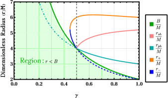
Figure 4: The figure above shows how the radius of the photon sphere ($r_{ph}$), the corresponding shadow radius ($r_{sh}$), and the innermost circular orbits ($r_{\pm}$) for massive particles in Janis-Newman-Winicour (JNW) spacetime depend on the parameter $\gamma$. Unlike other spacetimes, in this scenario, the shadow radius decreases monotonically as the photon sphere radius increases within the range $0.5\leq\gamma\leq 1$. The JNW spacetime features a singularity at $r=B\equiv r_{g}$, where $B=\dfrac{2M}{\gamma}$, $M$ being the Arnowitt-Deser-Misner (ADM) mass of the gravitating object. The green shaded area, i.e., the region $r<r_{g}=B$, represents an unphysical solution. Additionally, at $\gamma=0.50$, the photon sphere radius and shadow radius coincide, meaning $r_{ph}=r_{sh}=r_{g}=B$. The dashed blue line and dot-dashed cyan lines depict extended numerical solutions of $r_{-}$ and $r_{ph}$, which are unphysical.

6.3 Conversion factor for JNW spacetime

As discussed in previous section, the scattering of photon in plasma can affect the conversion factor. However, in 5.2, we also have discussed the possibility of neglecting the effect of such phenomena. For JNW spacetime in the parameter range $0.5\leq\gamma\leq 1$, one can always show that

$$0\leq\dfrac{1}{\sqrt{\mathcal{P}}\sqrt{f(r_{ph})}}\dfrac{r_{ph}}{M}=\left(2-\dfrac{1}{\gamma}\right)^{\frac{1-\gamma}{2}}\left(2+\dfrac{1}{\gamma}\right)^{\frac{1+\gamma}{2}}\leq 3$$ (106)

This result has also been depicted in 5. As a result, for this spacetime, one can readily show that 97 is indeed satisfied. Hence, we can ignore the scattering of photons inside the plasma for our further analysis.

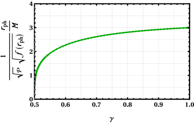
(a) Change in the scattering-limit factor has been shown for the range of the characteristic parameter $\gamma$ in range $(0.5,1)$.

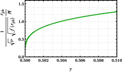
(b) Change in the scattering-limit factor has been shown for the range of the characteristic parameter $\gamma$ in range $(0.5,0.510)$.

Figure 5: Variation of the dimensionless scattering-limit-factor has been depicted with the change of the characteristic parameter $\gamma$ in the range $0.5\leq\gamma\leq 1$. One can observe that this factor monotonically increases from $0$ to $3$.

In 6, we have illustrated the variations of the conversion factor (CF), in the effective conversion regime, i.e, when $\Delta_{\rm osc}=2\Delta_{M}$, with the variation of dimensionless quantity $M\Delta_{\rm M}$ and dimensionless characteristic parameter $\gamma$.

In particular, in 6a and 6b, the variation of the conversion factor has been demonstrated while the characteristic parameter $\gamma$ has been varied, keeping the dimensionless quantity $M\Delta_{M}$ constant. One can observe that the change in conversion factor is more rapid in the range $0.50\lesssim\gamma\lesssim 0.60$. Although, for $\gamma>0.60$, the conversion factor monotonically increases, the rate of increase is much lower than the previously mentioned range of the parameter $\gamma$. As shown in 6c, for a fixed value of the characteristic parameter $\gamma$, the conversion factor increases monotonically with the increase in the value of dimensionless quantity $M\Delta_{M}$, and gradually approaches its peak value i.e. $25\%$ conversion. This phenomenon is explained by the selective conversion of photons that have a polarization aligned with the magnetic field. The production of photons with this polarization and axions occurs at an equal rate due to significant mixing. Examining 6c, it can also be noticed that for sufficiently high value of dimensionless quantity $M\Delta_{M}$ (in this case $M\Delta_{M}\sim 4-5$), the conversion rate almost approaches its peak value, seemingly irrespective of the value of the characteristic parameter $\gamma$. This can also be confirmed by examining 86.

In 6d, contour lines represent consistent levels of the conversion factor, emphasizing the areas in the parameter space where notable fluctuations in the conversion factor take place. Similarly, in 6e, the colour gradient illustrates the density of the conversion factor, providing insights into the places with large variance in conversion efficiency. From 6d and 6e, it is easily understood that the conversion factor is effectively enhanced for relatively high value of both $\gamma$ and $M\Delta_{M}$.

(a) Rapid increase in conversion factor has been depicted for minor variation of the characteristic parameter $\gamma$ near $\gamma=0.50$ for different fixed values of dimensionless quantity $M\Delta_{M}$.

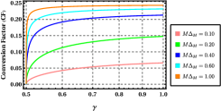
(b) Variation of the conversion factor with the change in characteristic parameter $\gamma$ has been shown for full range of the parameter, for various values of dimensionless quantity $M\Delta_{M}$.

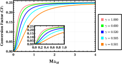
(c) With changes in the dimensionless quantity $M\Delta_{M}$, variations in the conversion factor have been demonstrated for different values of dimensionless parameter $\gamma$.

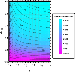
(d) This plot depicts the variation of the conversion factor in response to changes in two dimensionless parameters, $M\Delta_{M}$ and $\gamma$. Contour lines indicate constant levels of the conversion factor, highlighting the regions of the parameter space where significant changes in the conversion factor occur.

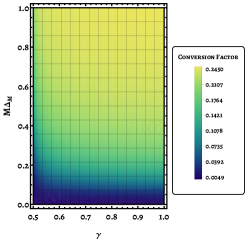
(e) This density plot illustrates the distribution of the conversion factor over the ranges of two dimensionless parameters, $M\Delta_{M}$ and $\gamma$. The colour gradient represents the density of the conversion factor, providing insights into the regions with significant variation in conversion efficiency.

Figure 6: In the instance of effective conversion, i.e. when $\Delta_{\rm osc}=2\Delta_{M}$, the variation of the conversion factor has been demonstrated in conjunction with the change of the dimension-less parameters $\gamma$ and dimensionless quantity $M\Delta_{M}$.

7 Dimming of the photon ring Luminosity

7.1 Dimming of the photon sphere

After we have determined the conversion factor, all that is required of us is to make a count of the photon numbers that have approached the photon sphere and then escaped to infinity. This will allow us to determine the number of photons that have been converted and the newly formed axion. With the help of 73 and 75, the photon count can be determined as

$$\dfrac{\differential^{2}N}{\differential t\differential\omega_{c}}=\mathfrak{L}^{0}_{\omega}\omega_{\rm obs}^{-1}\times 2\mathfrak{a}\left(\dfrac{b_{c}}{M}\right)^{2}\left(\dfrac{r_{ph}}{M}\right)\times\int_{x_{\rm in}}^{x_{\rm out}}\differential x_{e}\left[\dfrac{x_{e}^{-3/2}\mathcal{R}(x_{e})f(x_{e})}{\sqrt{\dfrac{x_{e}^{2}\mathcal{R}^{2}(x_{e})}{f(x_{e})}-\left(\dfrac{b_{c}}{r_{ph}}\right)^{2}}}\right]e^{-\dfrac{\omega_{\rm obs}}{T_{e,c}}\dfrac{x_{e}}{\sqrt{f(x_{e})}}}$$ (107)

where the variable $x$ is defined as $x=r/r_{ph}$ and the quantity $\mathfrak{L}^{0}_{\omega}$ is defined as

$$\mathfrak{L}^{0}_{\omega} =2\pi^{2}\epsilon^{2}M^{3}\left(\dfrac{4\alpha^{3}}{3\pi m_{e}}\right)\left(\dfrac{2\pi}{3m_{e}}\right)^{1/2}T_{e,c}^{-1/2}n_{e,c}^{2}\bar{g}_{ff}$$ (108)

$$=6.48\times 10^{27}{\rm erg.sec^{-1}.KeV^{-1}}\epsilon^{2}\left(\dfrac{M}{6.2\times 10^{9}M_{\odot}}\right)^{3}\left(\dfrac{T_{e,c}}{10^{11}K}\right)^{-1/2}\left(\dfrac{n_{e,c}}{10^{4}{\rm cm^{-3}}}\right)^{2}\bar{g}_{ff}$$ (109)

One should notice the fact, due to gravitational redshift, the observed frequency $\omega_{\rm obs}$ is directly connected to the frequency $\omega_{c}$ at the photon sphere as $\omega_{\rm obs}=\sqrt{f(r_{ph})}\omega_{c}$. As the distance of M87* is around $D\approx 16.8{\rm Mpc}$, the cosmological redshift of M87* can be calculated to be $\mathfrak{z}\approx\dfrac{H_{0}D}{c}\approx 0.004$, where $H_{0}$ is the present value of the Hubble parameter, which is considered to be $71{\rm km/s/Mpc}$ for our study. Within the local universe, galaxies, such as the Messier galaxy, generally have peculiar velocities that are normally in the range of a few hundred kilometres per second. However, while evaluating the prevailing gravitational redshift, we disregard minor factors like peculiar velocities and cosmic expansion.

We construct the following quantity to be the relative luminosity (RL) of photons prior to any conversion as

$$\dfrac{\mathfrak{L}^{\upgamma}_{\omega}}{\mathfrak{L}^{0}_{\omega}}\equiv\dfrac{\omega_{\rm obs}}{\mathfrak{L}^{0}_{\omega}}\left(\dfrac{\differential^{2}N}{\differential t\differential\omega_{c}}\right)=2\mathfrak{a}\left(\dfrac{b_{c}}{M}\right)^{2}\left(\dfrac{r_{ph}}{M}\right)\times\int_{x_{\rm in}}^{x_{\rm out}}\differential x_{e}\left[\dfrac{x_{e}^{-3/2}\mathcal{R}(x_{e})f(x_{e})}{\sqrt{\dfrac{x_{e}^{2}\mathcal{R}^{2}(x_{e})}{f(x_{e})}-\left(\dfrac{b_{c}}{r_{ph}}\right)^{2}}}\right]e^{-\dfrac{\omega_{\rm obs}}{T_{e,c}}\dfrac{x_{e}}{\sqrt{f(x_{e})}}}$$ (110)

The relative luminosity for the axions as generated throughout photon-axion conversion can be calculated by

$$\dfrac{\mathfrak{L}^{\upgamma\to\Phi}_{\omega}}{\mathfrak{L}^{0}_{\omega}}=\dfrac{\mathfrak{L}^{\upgamma}_{\omega}}{\mathfrak{L}^{0}_{\omega}}\dfrac{1}{4}\left(\dfrac{2\Delta_{\rm M}}{\Delta_{\rm osc}}\right)^{2}\left(\dfrac{1}{1+\mathcal{Y}^{2}}\right)$$ (111)

In 7, we have illustrated the spectral variation of the relative luminosity for both photons and axions with respect to the characteristic parameter $\gamma$. The spectrum has been standardized based on the undistorted relative brightness for a Schwarzschild black hole at very low frequencies. In 7a and 7b, the dotted lines show the relative luminosity of photons in the absence of photon conversion. While the solid lines show that the spectrum is reduced as a result of the fraction of photons becoming axions. The influence of the attenuation of the spectrum from its undistorted component becomes increasingly evident when the parameter is gradually reduced from its peak value $\gamma_{\rm max}=1$. From 7a and 7b, it can also be inferred that the percentage of attenuation along with initiation point of attenuation-frequency depends on the mass of axions. In 7c and 7d, the variation of axion spectra has been depicted for a set of three values of characteristic parameter $\gamma$. It is noticed that the spread of the band of axion spectra for axion mass $m_{\Phi}=10\rm~{}neV$ is narrower than that of the spectrum for axion mass $m_{\Phi}=1\rm~{}neV$.

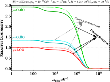
(a) The relative brightness spectra of photons, both dimmed and undimmed, have been shown with the axion mass assumed to be $m_{\Phi}=1~{}~{}\rm neV$ for different set of values of characteristic parameter $\gamma$.

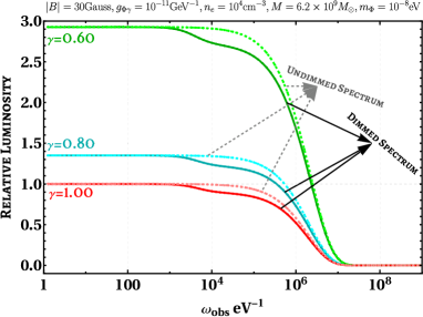
(b) The relative luminosity spectrum of photons has been illustrated, considering the axion mass as $m_{\Phi}=10~{}~{}\rm neV$, with both dimmed and undimmed conditions for different set of values of characteristic parameter $\gamma$.

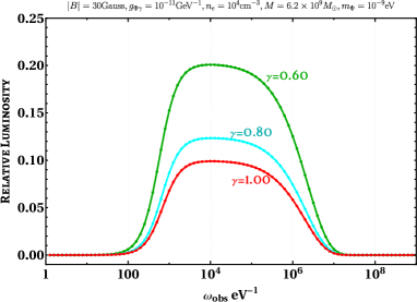
(c) The relative brightness spectrum of axions is shown with an axion mass of $m_{\Phi}=1~{}~{}\rm neV$, with varying values of the characteristic parameter $\gamma$.

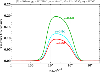
(d) The relative brightness spectrum of axions is shown with an axion mass of $m_{\Phi}=10~{}~{}\rm neV$, with varying values of the characteristic parameter $\gamma$.

Figure 7: The relative luminosity spectra of photons has been depicted both before (using dotted lines) and after (using solid lines) the conversion of photons into axions. In this scenario, we have made the assumption that the magnetic field linked to the compact object is $|\mathbf{B}|=30$ Gauss, the coupling between the axion and photon is $g_{\Phi\upgamma}=10^{-11}\rm GeV^{-1}$, electron number density to be $n_{e}=10^{4}\rm cm^{-3}$ and the mass of the compact object is $M=6.2\times 10^{9}M_{\odot}$. Plots have been exhibited for two distinct mass values of axions.

In 8 we have demonstrated the continuous variation of relative luminosity spectrum with the simultaneous variation of characteristic parameter $\gamma$ in the specified range of $0.5<\gamma<1$, assuming axion mass to be $1~{}\rm neV$. In 8a and 8b we have depicted the variation of photon spectra without the photon-axion conversion and with photon-axion conversion, respectively. Axion spectrum arising due to the photon-axion conversion phenomena has been illustrated in 8c. This photon luminosity is suppressed at higher frequency because there are so few high-temperature electrons in the electromagnetic plasma that can produce photons at such high frequencies.

The condition of flat part of the photon spectrum can be understood with the help of 75. The exponential factor, arising in the equation 75, can be put to unity if

$$\dfrac{\omega_{e}}{T_{e}}=\dfrac{\omega_{c}}{T_{e,c}}\sqrt{\dfrac{f(r_{c})}{f(r_{e})}}\left(\dfrac{r_{e}}{r_{ph}}\right)\ll 1$$ (112)

In such circumstances, the Relative Luminosity (RL) reaches its maximum value and the spectrum approaches an almost flat region.

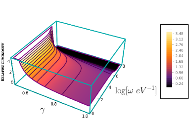
(a) Variation of relative luminosity of photons has been depicted before the conversion of photons into axions.

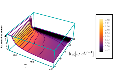
(b) Variation of relative luminosity of photons has been depicted after the conversion of photons into axions.

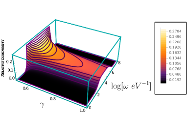
(c) Variation of relative luminosity of axions produced via photon-to-axion conversion process.

Figure 8: The relative luminosity spectra of photons and axions have been illustrated, with the state before and after the conversion of photons into axions. It is assumed that the magnetic field connected to the compact object is $|\mathbf{B}|=30~{}~{}\rm Gauss$, the interaction between the axion and photon is $10^{-11}~{}~{}\rm GeV^{-1}$, and the electron density is $n_{e}=10^{4}~{}~{}\rm cm^{3}$. The mass of the compact object is $M=6.2\times 10^{9}M_{\odot}$. The plots are illustrated for axion mass value $m_{\Phi}=1~{}\rm neV$.

7.2 Required resolution of the image

We expect that the photon-axion conversion will affect the observed photon spectrum. However, since the conversion occurs only near the photon sphere, we should note that only the spectrum near the photon sphere can be distorted. Thus, to observe the spectral distortion, we need to resolve the near-horizon region itself. Although the Event Horizon Telescope has effectively captured images of the structure near the compact object using radio waves, it is not currently equipped to perform high-resolution studies in the X-ray and gamma-ray ranges. Under these circumstances, the overall brightness emanating from the area surrounding the compact object will be significant. Total luminosity of photons emanating from a region $r_{\rm isco}<r_{e}<\mathscr{R}$ can be provided by the following approximate formula

$$\mathcal{L}_{\rm total} =4\pi\int_{r_{\rm isco}}^{\mathscr{R}}\differential r_{e}~{}r_{e}^{2}\dfrac{dW}{\differential r_{e}\differential\omega_{e}\differential V_{e}}\sim\dfrac{16}{\epsilon^{2}}\left(\dfrac{r_{ph}}{M}\right)^{3}\left[\sqrt{\left(\dfrac{\mathscr{R}}{r_{ph}}\right)}-\sqrt{\left(\dfrac{r_{\rm isco}}{r_{ph}}\right)}\right]\mathcal{L}_{\omega}^{0}$$ (113)

where $r_{\rm isco}$ represents the radius of innermost stable circular orbit. From 113, one can conclude that the majority of the overall brightness will be attributed to the emission originating from the area beyond photon sphere. As a result, the reduction in brightness caused by the conversion will be negligible. We know that the Chandra observatory has angular resolution of order of arc-sec and hence unable to detect the dimming phenomena for M87* since it observes the area beyond the photon sphere. The observation of such dimming can be possible only if we increase the resolution of the captured image of the compact object. To achieve such precision, we need to track the photons near the photon sphere of the compact object, i.e, over a region where $\mathscr{R}\sim r_{ph}$. The required resolution for such scenario is

$$\theta=\evaluated{\dfrac{\mathscr{R}}{D}}_{\gamma=1}\lesssim 10^{-5}{\rm arcsec}\left(\dfrac{M}{6.2\times 10^{9}M_{\odot}}\right)\left(\dfrac{16.8{\rm Mpc}}{D}\right)$$ (114)

where $D$ is the distance of compact object from the observer. So, for M87* compact object, even for X-ray and gamma-ray, we need the angular resolution $\theta\lesssim 10~{}\upmu{\rm as}$. In 7 and 8, The expected energy spectrum are illustrated with multiple examples. The horizontal axis represent the frequency we observe, denoted as $\omega_{\rm obs}$. This frequency is connected to the frequency at the photon sphere, denoted as $\omega_{c}$, by the equation $\omega_{\rm obs}=\sqrt{f(r_{ph})}\omega_{c}$, where $\sqrt{f(r_{ph})}$ is a constant factor accounting for gravitational redshift. We disregarded further minor influences, such as peculiar velocities and cosmic expansion. In each of such scenarios, the spectral luminosity has been normalised by the infrared value for $\gamma=1$ case. We also assumed that the photons are created by thermal bremsstrahlung of the gas spread over a spherical region (starting from $r_{\rm isco}$) around the compact object. One should remember that the cut-off frequency of the spectrum is at around $\omega_{\rm obs}\sim T_{e,c}\sim 10^{7}~{}\rm eV$ due to the exponential suppression factor in 107. For $\theta\simeq 1~{}\rm arcsec$, due to the lack of angular resolution, we are unable to discover any spectral distortion in the X-ray spectrum. On the other hand, when $\theta$ equals around few $\rm\upmu as$, we are able to resolve the photon sphere itself, which allows us to observe the reduction in the brightness for the X-ray spectrum.

8 Conclusion

If one consider the existence of the axions in the universe, photons that pass through a magnetic field can undergo a conversion process into axions due to the presence of a coupling term $\dfrac{1}{4}g_{\Phi\upgamma}\Phi F^{\mu\nu}\tilde{F}^{\mu\nu}$ in the Lagrangian. It is widely recognized that active galactic nuclei contain a compact object at their centre. Furthermore, it is anticipated that substantial magnetic fields would be present in the vicinity of the compact object. Nevertheless, it is impossible to avoid the potential existence of a naked singularity with sufficiently strong magnetic field at the core of the galaxy. From 47, we determine that the propagation length necessary for conversion is of the order of a milli-parsec, which is comparable to the Schwarzschild radius of a supermassive compact object with a mass of $10^{9}~{}M_{\odot}$, when we take into account an associated magnetic field of approximately $|B|\sim 30$ Gauss, an axion-photon coupling of $g_{\Phi\upgamma}\sim 10^{-11}~{}\rm GeV^{-1}$, and an electron number density of $10^{4}~{}\rm cm^{-3}$. At first glance, it appears that the magnetic field must be sustained in the radial direction throughout the conversion length. Nevertheless, photons can orbit a photon sphere of the compact object for a specific amount of time. The magnetic field is automatically maintained during propagation due to the fact that such orbiting particles maintain a nearly constant radius. Therefore, it is anticipated that the conversion of photons into axions would take place with high efficiency in the vicinity of the compact object.

Our investigations further show that photons in the X-ray and gamma-ray spectra can be efficiently converted into axions with masses less than $100~{}\rm neV$. Therefore, by using electromagnetic waves to study the area surrounding the compact object, it may be possible to detect a decrease in the brightness of the photon ring in those specific wavelengths, as long as future advancements allow for a high level of detail. Larger values of the mass of a gravitating object correspond to increased dimming, making the compact object like M87* prominent candidates for detecting photon ring dimming. While the Event Horizon Telescope has succeeded in imaging the region in the radio band, acquiring such high-resolution observations in the X-ray and gamma-ray bands remains a problem. This study presents the determination of the distance travelled by photons along the curved path of a spherically symmetric spacetime. This allows us to compute the likelihood of photon-axion conversion in the spacetime of a naked singularity with spherical symmetry, assuming the mass of the compact object is already known. By choosing a more generalised spacetime metric in 3, we have broadened the notions presented in existing literature [163, 76], leading to a more comprehensive approach. However, after achieving the generalisation, we have applied the results for a naked singularity solution. There are various naked singularity in literature. Out of these, the most important naked singularity solution is Janis-Newman-Winicour spacetime, which has been considered here for our analysis. For the sake of simplicity, in our analysis we have assumed that the magnetic field and plasma density are uniform in the vicinity of the photon sphere. Since our analysis is applicable for large parameter range, we expect our analysis to work in relatively more realistic situations where inhomogeneity in magnetic field or plasma density are present. The sources that release photons through a radiative bremsstrahlung process are believed to exist outside the photon sphere. The brightness is mostly influenced by the lower limit of the integral in 73 rather than the upper limit. Therefore, the distance we choose from the centre of the compact object is of greater significance. In this study, we have defined the lower limit as the innermost stable circular orbit (ISCO). Another important thing to notice is that the “scattering-limit-factor” ($\mathfrak{S}$) as defined in 97 has an upper limit $\mathfrak{S}_{\rm upp}=3$ and monotonically decreases to $\mathfrak{S}_{\rm low}=0$ as we vary the characteristic parameter $\gamma$ of JNW spacetime from $\gamma=1$ to $\gamma=0.5$. So the impact of the effect of scattering of photons to determine the conversion factor is more prominent for the Schwarzschild black hole than that of the JNW naked singularity. In fact, for JNW spacetime with characteristic parameter $\gamma$ very near to limiting value $\gamma_{\rm low}=0.5$, one can safely ignore the effect of scattering phenomena entirely, even for very small value of photon mean free path.

There are other avenues to explore beyond the current project. One approach is to incorporate the rotational motion of the compact object. The rotating compact object exhibits the intriguing phenomenon of photons orbiting at two distinct radii on the equatorial plane. Due to the gravitational redshift experienced by photons released from various distances, the conversion into axions at those radii may result in dimming at different frequencies. It is also crucial to investigate the impact of photon-axion conversion on the polarisation of light emitted from the photon sphere. It is also worth studying conversion not only in the background of the magnetic field but also in the background of the axion[171, 172], since they are the potential candidate for dark matter and may be produced due to superradiance instability of the compact object [173, 174]. Another possible direction is to test the effect of conversion mechanism for the regular compact objects and even for regularised version of JNW spacetime[175] and to explore astrophysical aspects and the possibility of distinguishing such solutions from singular ones.

References

- [1] R. D. Peccei and H. R. Quinn, “Cp conservation in the presence of instantons,” Phys. Rev. Lett 38 no. 328, (1977) 1440–1443.
- [2] S. Weinberg, “A new light boson?,” Physical Review Letters 40 no. 4, (1978) 223.
- [3] F. Wilczek, “Problem of strong p and t invariance in the presence of instantons,” Physical Review Letters 40 no. 5, (1978) 279.
- [4] J. E. Kim, “Weak-interaction singlet and strong cp invariance,” Physical Review Letters 43 no. 2, (1979) 103.
- [5] M. A. Shifman, A. Vainshtein, and V. I. Zakharov, “Can confinement ensure natural cp invariance of strong interactions?,” Nuclear Physics B 166 no. 3, (1980) 493–506.
- [6] M. Dine, W. Fischler, and M. Srednicki, “A simple solution to the strong cp problem with a harmless axion,” Physics letters B 104 no. 3, (1981) 199–202.
- [7] A. R. Zhitnitsky, “On Possible Suppression of the Axion Hadron Interactions. (In Russian),” Sov. J. Nucl. Phys. 31 (1980) 260.
- [8] J. P. Conlon, “The QCD axion and moduli stabilisation,” JHEP 05 (2006) 078, arXiv:hep-th/0602233.
- [9] K. Freese, J. A. Frieman, and A. V. Olinto, “Natural inflation with pseudo nambu-goldstone bosons,” Physical Review Letters 65 no. 26, (1990) 3233.
- [10] J. E. Kim, H. P. Nilles, and M. Peloso, “Completing natural inflation,” Journal of Cosmology and Astroparticle Physics 2005 no. 01, (2005) 005.
- [11] S. Dimopoulos, S. Kachru, J. McGreevy, and J. G. Wacker, “N-flation,” Journal of Cosmology and Astroparticle Physics 2008 no. 08, (2008) 003.
- [12] J. Preskill, M. B. Wise, and F. Wilczek, “Cosmology of the invisible axion,” Physics Letters B 120 no. 1-3, (1983) 127–132.
- [13] L. F. Abbott and P. Sikivie, “A cosmological bound on the invisible axion,” Physics Letters B 120 no. 1-3, (1983) 133–136.
- [14] M. Dine and W. Fischler, “The not-so-harmless axion,” Physics Letters B 120 no. 1-3, (1983) 137–141.
- [15] L. Hui, J. P. Ostriker, S. Tremaine, and E. Witten, “Ultralight scalars as cosmological dark matter,” Physical Review D 95 no. 4, (2017) 043541.
- [16] F. Chadha-Day, J. Ellis, and D. J. Marsh, “Axion dark matter: What is it and why now?,” Science advances 8 no. 8, (2022) eabj3618.
- [17] J. A. Frieman, C. T. Hill, A. Stebbins, and I. Waga, “Cosmology with ultralight pseudo nambu-goldstone bosons,” Physical Review Letters 75 no. 11, (1995) 2077.
- [18] K. Choi, “String or m theory axion as a quintessence,” Physical Review D 62 no. 4, (2000) 043509.
- [19] E. J. Copeland, M. Sami, and S. Tsujikawa, “Dynamics of dark energy,” International Journal of Modern Physics D 15 no. 11, (2006) 1753–1935.
- [20] D. J. E. Marsh, “Axion Cosmology,” Phys. Rept. 643 (2016) 1–79, arXiv:1510.07633 [astro-ph.CO].
- [21] P. Sikivie, “AXIONS IN COSMOLOGY,” in 14th Summer School on Particle Physics, pp. 1–40. 1983.
- [22] P. Sikivie, “Experimental tests of the "invisible" axion,” Phys. Rev. Lett. 51 (1983) 1415. Erratum in Phys. Rev. Lett. 52, 695 (1984).
- [23] G. Raffelt and L. Stodolsky, “Mixing of the photon with low-mass particles,” Physical Review D 37 no. 5, (1988) 1237.
- [24] A. A. Anselm, “Experimental test for arion-photon oscillations in a homogeneous constant magnetic field,” Physical Review D 37 no. 7, (1988) 2001.
- [25] G. G. Raffelt, “Particle physics from stars,” Annual Review of Nuclear and Particle Science 49 no. 1, (1999) 163–216.
- [26] L. Maiani, R. Petronzio, and E. Zavattini, “Effects of nearly massless, spin-zero particles on light propagation in a magnetic field,” Physics Letters B 175 no. 3, (1986) 359–363.
- [27] E. Armengaud, F. Avignone, M. Betz, P. Brax, P. Brun, G. Cantatore, J. Carmona, G. Carosi, F. Caspers, S. Caspi, et al., “Conceptual design of the international axion observatory (iaxo),” Journal of Instrumentation 9 no. 05, (2014) T05002.
- [28] C. collaboration, “New cast limit on the axion–photon interaction,” Nature Physics 13 no. 6, (2017) 584–590.
- [29] S. J. Asztalos, G. Carosi, C. Hagmann, D. Kinion, K. Van Bibber, M. Hotz, L. Rosenberg, G. Rybka, J. Hoskins, J. Hwang, et al., “Squid-based microwave cavity search for dark-matter axions,” Physical review letters 104 no. 4, (2010) 041301.
- [30] C. Csaki, N. Kaloper, and J. Terning, “Dimming supernovae without cosmic acceleration,” Physical Review Letters 88 no. 16, (2002) 161302.
- [31] C. Csaki, N. Kaloper, and J. Terning, “Effects of the intergalactic plasma on supernova dimming via photon–axion oscillations,” Physics Letters B 535 no. 1-4, (2002) 33–36.
- [32] C. Deffayet, D. Harari, J.-P. Uzan, and M. Zaldarriaga, “Dimming of supernovae by photon-pseudoscalar conversion and the intergalactic plasma,” Physical Review D 66 no. 4, (2002) 043517.
- [33] Y. Grossman, S. Roy, and J. Zupan, “Effects of initial axion production and photon–axion oscillation on type ia supernova dimming,” Physics Letters B 543 no. 1-2, (2002) 23–28.
- [34] A. Mirizzi, J. Redondo, and G. Sigl, “Constraining resonant photon-axion conversions in the early universe,” Journal of Cosmology and Astroparticle Physics 2009 no. 08, (2009) 001.
- [35] H. Tashiro, J. Silk, and D. J. Marsh, “Constraints on primordial magnetic fields from cmb distortions in the axiverse,” Physical Review D 88 no. 12, (2013) 125024.
- [36] G. Galanti, L. Nava, M. Roncadelli, F. Tavecchio, and G. Bonnoli, “Observability of the very-high-energy emission from grb 221009a,” Physical Review Letters 131 no. 25, (2023) 251001.
- [37] J. P. Conlon and F. V. Day, “3.55 keV photon lines from axion to photon conversion in the Milky Way and M31,” JCAP 11 (2014) 033, arXiv:1404.7741 [hep-ph].
- [38] S. V. Troitsky, “Parameters of axion-like particles required to explain high-energy photons from grb 221009a,” JETP Letters 116 no. 11, (2022) 767–770.
- [39] A. Baktash, D. Horns, and M. Meyer, “Interpretation of multi-TeV photons from GRB221009A,” arXiv:2210.07172 [astro-ph.HE].
- [40] W. Lin and T. T. Yanagida, “Electroweak axion in light of grb221009a,” Chinese Physics Letters 40 no. 6, (2023) 069801.
- [41] M. Gonzalez, D. A. Rojas, A. Pratts, S. Hernandez-Cadena, N. Fraija, R. Alfaro, Y. P. Araujo, and J. Montes, “Grb 221009a: A light dark matter burst or an extremely bright inverse compton component?,” The Astrophysical Journal 944 no. 2, (2023) 178.
- [42] S. Nakagawa, F. Takahashi, M. Yamada, and W. Yin, “Axion dark matter from first-order phase transition, and very high energy photons from grb 221009a,” Physics Letters B 839 (2023) 137824.
- [43] P. Carenza and M. C. D. Marsh, “On ALP scenarios and GRB 221009A,” arXiv:2211.02010 [astro-ph.HE].
- [44] L. Wang and B.-Q. Ma, “Axion-photon conversion of grb221009a,” Physical Review D 108 no. 2, (2023) 023002.
- [45] J. P. Conlon, M. C. D. Marsh, and A. J. Powell, “Galaxy cluster thermal x-ray spectra constrain axionlike particles,” Phys. Rev. D 93 no. 12, (2016) 123526, arXiv:1509.06748 [hep-ph].
- [46] M. Berg, J. P. Conlon, F. Day, N. Jennings, S. Krippendorf, A. J. Powell, and M. Rummel, “Constraints on Axion-Like Particles from X-ray Observations of NGC1275,” Astrophys. J. 847 no. 2, (2017) 101, arXiv:1605.01043 [astro-ph.HE].
- [47] J. P. Conlon, F. Day, N. Jennings, S. Krippendorf, and M. Rummel, “Constraints on Axion-Like Particles from Non-Observation of Spectral Modulations for X-ray Point Sources,” JCAP 07 (2017) 005, arXiv:1704.05256 [astro-ph.HE].
- [48] D. Hooper and P. D. Serpico, “Detecting axionlike particles with gamma ray telescopes,” Physical Review Letters 99 no. 23, (2007) 231102.
- [49] K. A. Hochmuth and G. Sigl, “Effects of axion-photon mixing on gamma-ray spectra from magnetized astrophysical sources,” Physical Review D—Particles, Fields, Gravitation, and Cosmology 76 no. 12, (2007) 123011.
- [50] A. De Angelis, O. Mansutti, and M. Roncadelli, “Axion-like particles, cosmic magnetic fields and gamma-ray astrophysics,” Physics Letters B 659 no. 5, (2008) 847–855.
- [51] A. Abramowski, F. Acero, F. Aharonian, F. Ait Benkhali, A. Akhperjanian, E. Angüner, G. Anton, S. Balenderan, A. Balzer, A. Barnacka, et al., “Constraints on axionlike particles with hess from the irregularity of the pks 2155-304 energy spectrum,” Physical Review D—Particles, Fields, Gravitation, and Cosmology 88 no. 10, (2013) 102003.
- [52] M. Ajello, A. Albert, B. Anderson, L. Baldini, G. Barbiellini, D. Bastieri, R. Bellazzini, E. Bissaldi, R. Blandford, E. Bloom, et al., “Search for spectral irregularities due to photon–axionlike-particle oscillations with the fermi large area telescope,” Physical Review Letters 116 no. 16, (2016) 161101.
- [53] M. D. Marsh, H. R. Russell, A. C. Fabian, B. R. McNamara, P. Nulsen, and C. S. Reynolds, “A new bound on axion-like particles,” Journal of Cosmology and Astroparticle Physics 2017 no. 12, (2017) 036.
- [54] C. Zhang, Y.-F. Liang, S. Li, N.-H. Liao, L. Feng, Q. Yuan, Y.-Z. Fan, and Z.-Z. Ren, “New bounds on axionlike particles from the fermi large area telescope observation of pks 2155-304,” Physical Review D 97 no. 6, (2018) 063009.
- [55] C. S. Reynolds, M. D. Marsh, H. R. Russell, A. C. Fabian, R. Smith, F. Tombesi, and S. Veilleux, “Astrophysical limits on very light axion-like particles from chandra grating spectroscopy of ngc 1275,” The Astrophysical Journal 890 no. 1, (2020) 59.
- [56] M. Simet, D. Hooper, and P. D. Serpico, “Milky way as a kiloparsec-scale axionscope,” Physical Review D—Particles, Fields, Gravitation, and Cosmology 77 no. 6, (2008) 063001.
- [57] A. Mirizzi and D. Montanino, “Stochastic conversions of tev photons into axion-like particles in extragalactic magnetic fields,” Journal of Cosmology and Astroparticle Physics 2009 no. 12, (2009) 004.
- [58] M. Meyer, D. Horns, and M. Raue, “First lower limits on the photon-axion-like particle coupling from very high energy gamma-ray observations,” Physical Review D—Particles, Fields, Gravitation, and Cosmology 87 no. 3, (2013) 035027.
- [59] S. Angus, J. P. Conlon, M. C. D. Marsh, A. J. Powell, and L. T. Witkowski, “Soft X-ray Excess in the Coma Cluster from a Cosmic Axion Background,” JCAP 09 (2014) 026, arXiv:1312.3947 [astro-ph.HE].
- [60] J. P. Conlon and S. Krippendorf, “Axion decay constants away from the lamppost,” JHEP 04 (2016) 085, arXiv:1601.00647 [hep-th].
- [61] J. P. Conlon and M. C. D. Marsh, “Excess Astrophysical Photons from a 0.1–1 keV Cosmic Axion Background,” Phys. Rev. Lett. 111 no. 15, (2013) 151301, arXiv:1305.3603 [astro-ph.CO].
- [62] J. P. Conlon and M. C. D. Marsh, “The Cosmophenomenology of Axionic Dark Radiation,” JHEP 10 (2013) 214, arXiv:1304.1804 [hep-ph].
- [63] M. J. Dolan, F. J. Hiskens, and R. R. Volkas, “Advancing globular cluster constraints on the axion-photon coupling,” Journal of Cosmology and Astroparticle Physics 2022 no. 10, (2022) 096.
- [64] C. Dessert, D. Dunsky, and B. R. Safdi, “Upper limit on the axion-photon coupling from magnetic white dwarf polarization,” Physical Review D 105 no. 10, (2022) 103034.
- [65] LIGO Scientific, Virgo Collaboration, B. P. Abbott et al., “Observation of Gravitational Waves from a Binary Black Hole Merger,” Phys. Rev. Lett. 116 no. 6, (2016) 061102, arXiv:1602.03837 [gr-qc].
- [66] LIGO Scientific, Virgo Collaboration, B. P. Abbott et al., “GW170817: Observation of Gravitational Waves from a Binary Neutron Star Inspiral,” Phys. Rev. Lett. 119 no. 16, (2017) 161101, arXiv:1710.05832 [gr-qc].
- [67] Event Horizon Telescope Collaboration, V. L. Fish, K. Akiyama, K. L. Bouman, A. A. Chael, M. D. Johnson, S. S. Doeleman, L. Blackburn, J. F. C. Wardle, and W. T. Freeman, “Observing—and Imaging—Active Galactic Nuclei with the Event Horizon Telescope,” Galaxies 4 no. 4, (2016) 54, arXiv:1607.03034 [astro-ph.IM].
- [68] Event Horizon Telescope Collaboration, K. Akiyama et al., “First M87 Event Horizon Telescope Results. I. The Shadow of the Supermassive Black Hole,” Astrophys. J. Lett. 875 (2019) L1, arXiv:1906.11238 [astro-ph.GA].
- [69] Event Horizon Telescope Collaboration, K. Akiyama et al., “First M87 Event Horizon Telescope Results. II. Array and Instrumentation,” Astrophys. J. Lett. 875 no. 1, (2019) L2, arXiv:1906.11239 [astro-ph.IM].
- [70] Event Horizon Telescope Collaboration, K. Akiyama et al., “First M87 Event Horizon Telescope Results. III. Data Processing and Calibration,” Astrophys. J. Lett. 875 no. 1, (2019) L3, arXiv:1906.11240 [astro-ph.GA].
- [71] Event Horizon Telescope Collaboration, K. Akiyama et al., “First M87 Event Horizon Telescope Results. IV. Imaging the Central Supermassive Black Hole,” Astrophys. J. Lett. 875 no. 1, (2019) L4, arXiv:1906.11241 [astro-ph.GA].
- [72] Event Horizon Telescope Collaboration, K. Akiyama et al., “First M87 Event Horizon Telescope Results. V. Physical Origin of the Asymmetric Ring,” Astrophys. J. Lett. 875 no. 1, (2019) L5, arXiv:1906.11242 [astro-ph.GA].
- [73] Event Horizon Telescope Collaboration, K. Akiyama et al., “First M87 Event Horizon Telescope Results. VI. The Shadow and Mass of the Central Black Hole,” Astrophys. J. Lett. 875 no. 1, (2019) L6, arXiv:1906.11243 [astro-ph.GA].
- [74] Event Horizon Telescope Collaboration, K. Akiyama et al., “First M87 Event Horizon Telescope Results. VII. Polarization of the Ring,” Astrophys. J. Lett. 910 no. 1, (2021) L12, arXiv:2105.01169 [astro-ph.HE].
- [75] Event Horizon Telescope Collaboration, K. Akiyama et al., “First M87 Event Horizon Telescope Results. VIII. Magnetic Field Structure near The Event Horizon,” Astrophys. J. Lett. 910 no. 1, (2021) L13, arXiv:2105.01173 [astro-ph.HE].
- [76] K. Nomura, K. Saito, and J. Soda, “Observing axions through photon ring dimming of black holes,” Phys. Rev. D 107 no. 12, (2023) 123505, arXiv:2212.03020 [hep-ph].
- [77] S. Roy, P. Sarkar, S. Sau, and S. SenGupta, “Exploring axions through the photon ring of a spherically symmetric black hole,” JCAP 11 (2023) 099, arXiv:2310.05908 [gr-qc].
- [78] X. Y. Chew, I. G. Choi, H. J. Kim, and D.-h. Yeom, “Can a naked singularity be formed during the gravitational collapse of a Janis-Newman-Winicour solution?,” arXiv:2408.03016 [gr-qc].
- [79] C.-M. Chen, C.-C. Huang, S. P. Kim, and C.-Y. Wei, “Catastrophic Emission of Charges from Near-Extremal Rotating Charged Nariai Black Holes,” arXiv:2408.12343 [hep-th].
- [80] P. S. Joshi and I. H. Dwivedi, “Naked singularities in spherically symmetric inhomogeneous Tolman-Bondi dust cloud collapse,” Phys. Rev. D 47 (1993) 5357–5369, arXiv:gr-qc/9303037.
- [81] S. L. Shapiro and S. A. Teukolsky, “Formation of naked singularities: The violation of cosmic censorship,” Phys. Rev. Lett. 66 (Feb, 1991) 994–997. https://link.aps.org/doi/10.1103/PhysRevLett.66.994.
- [82] B. Waugh and K. Lake, “Strengths of Shell Focusing Singularities in Marginally Bound Collapsing Selfsimilar Tolman Space-times,” Phys. Rev. D 38 (1988) 1315–1316.
- [83] A. Ori and T. Piran, “Naked singularities in self-similar spherical gravitational collapse,” Phys. Rev. Lett. 59 (Nov, 1987) 2137–2140. https://link.aps.org/doi/10.1103/PhysRevLett.59.2137.
- [84] R. Mizuno, S. Ohashi, and T. Shiromizu, “Violation of cosmic censorship in the gravitational collapse of a dust cloud in five dimensions,” PTEP 2016 no. 10, (2016) 103E03, arXiv:1607.02698 [gr-qc].
- [85] T. Harada, “Gravitational collapse and naked singularities,” Pramana 63 (2004) 741–754, arXiv:gr-qc/0407109.
- [86] R. Giambo, F. Giannoni, G. Magli, and P. Piccione, “Naked singularities in the gravitational collapse of barotropic spherical fluids,” Gen. Rel. Grav. 36 (2004) 1279–1298, arXiv:gr-qc/0303043.
- [87] D. M. Eardley and L. Smarr, “Time functions in numerical relativity: Marginally bound dust collapse,” Phys. Rev. D 19 (Apr, 1979) 2239–2259. https://link.aps.org/doi/10.1103/PhysRevD.19.2239.
- [88] K. Lake, “Naked singularities in gravitational collapse which is not self-similar,” Phys. Rev. D 43 (Feb, 1991) 1416–1417. https://link.aps.org/doi/10.1103/PhysRevD.43.1416.
- [89] R. Goswami and P. S. Joshi, “Spherical gravitational collapse in N-dimensions,” Phys. Rev. D 76 (2007) 084026, arXiv:gr-qc/0608136.
- [90] T. Harada, H. Iguchi, and K.-i. Nakao, “Naked singularity formation in the collapse of a spherical cloud of counter rotating particles,” Phys. Rev. D 58 (1998) 041502, arXiv:gr-qc/9805071.
- [91] P. S. Joshi, N. Dadhich, and R. Maartens, “Why do naked singularities form in gravitational collapse?,” Phys. Rev. D 65 (2002) 101501, arXiv:gr-qc/0109051.
- [92] C. Chakraborty, S. Bhattacharyya, and P. S. Joshi, “Low mass naked singularities from dark core collapse,” JCAP 07 (2024) 053, arXiv:2405.08758 [astro-ph.HE].
- [93] P. Rudra, “Gravitational collapse in energy-momentum squared gravity: Nature of singularities,” Nucl. Phys. B 1000 (2024) 116461, arXiv:2402.07957 [gr-qc].
- [94] V. Vertogradov, “The eternal naked singularity formation in the case of gravitational collapse of generalized Vaidya space–time,” Int. J. Mod. Phys. A 33 no. 17, (2018) 1850102, arXiv:2210.16131 [gr-qc].
- [95] J.-Q. Guo, P. S. Joshi, R. Narayan, and L. Zhang, “Accretion disks around naked singularities,” Class. Quant. Grav. 38 no. 3, (2021) 035012, arXiv:2011.06154 [gr-qc].
- [96] R. Shaikh and P. S. Joshi, “Can we distinguish black holes from naked singularities by the images of their accretion disks?,” JCAP 10 (2019) 064, arXiv:1909.10322 [gr-qc].
- [97] R. Penrose, “Gravitational collapse: The role of general relativity,” Riv. Nuovo Cim. 1 (1969) 252–276.
- [98] W. Kluźniak and T. Krajewski, “Outflows from naked singularities, infall through the black hole horizon: hydrodynamic simulations of accretion in the Reissner-Nordström space-time,” arXiv:2408.08359 [astro-ph.HE].
- [99] Z. Kovacs and T. Harko, “Can accretion disk properties observationally distinguish black holes from naked singularities?,” Phys. Rev. D 82 (2010) 124047, arXiv:1011.4127 [gr-qc].
- [100] M. Blaschke and Z. Stuchlík, “Efficiency of the Keplerian accretion in braneworld Kerr-Newman spacetimes and mining instability of some naked singularity spacetimes,” Phys. Rev. D 94 no. 8, (2016) 086006, arXiv:1610.07462 [gr-qc].
- [101] Z. Stuchlik and J. Schee, “Appearance of Keplerian discs orbiting Kerr superspinars,” Class. Quant. Grav. 27 (2010) 215017, arXiv:1101.3569 [gr-qc].
- [102] C. Bambi, K. Freese, T. Harada, R. Takahashi, and N. Yoshida, “Accretion process onto super-spinning objects,” Phys. Rev. D 80 (2009) 104023, arXiv:0910.1634 [gr-qc].
- [103] P. S. Joshi, D. Malafarina, and R. Narayan, “Equilibrium configurations from gravitational collapse,” Class. Quant. Grav. 28 (2011) 235018, arXiv:1106.5438 [gr-qc].
- [104] P. Pradhan and P. Majumdar, “Circular Orbits in Extremal Reissner Nordstrom Spacetimes,” Phys. Lett. A 375 (2011) 474–479, arXiv:1001.0359 [gr-qc].
- [105] D. Pugliese, H. Quevedo, and R. Ruffini, “Equatorial circular motion in Kerr spacetime,” Phys. Rev. D 84 (2011) 044030, arXiv:1105.2959 [gr-qc].
- [106] D. Tahelyani, A. B. Joshi, D. Dey, and P. S. Joshi, “Comparing thin accretion disk properties of naked singularities and black holes,” Phys. Rev. D 106 no. 4, (2022) 044036, arXiv:2205.04055 [gr-qc].
- [107] R. K. Karimov, R. N. Izmailov, A. A. Potapov, and K. K. Nandi, “Can accretion properties distinguish between a naked singularity, wormhole and black hole?,” Eur. Phys. J. C 80 no. 12, (2020) 1138, arXiv:2012.13564 [gr-qc].
- [108] G. Gyulchev, J. Kunz, P. Nedkova, T. Vetsov, and S. Yazadjiev, “Observational signatures of strongly naked singularities: image of the thin accretion disk,” Eur. Phys. J. C 80 no. 11, (2020) 1017, arXiv:2003.06943 [gr-qc].
- [109] K. Hioki and K.-i. Maeda, “Measurement of the Kerr Spin Parameter by Observation of a Compact Object’s Shadow,” Phys. Rev. D 80 (2009) 024042, arXiv:0904.3575 [astro-ph.HE].
- [110] L. Yang and Z. Li, “Shadow of a dressed black hole and determination of spin and viewing angle,” Int. J. Mod. Phys. D 25 no. 02, (2015) 1650026, arXiv:1511.00086 [astro-ph.HE].
- [111] R. Takahashi, “Shapes and positions of black hole shadows in accretion disks and spin parameters of black holes,” J. Korean Phys. Soc. 45 (2004) S1808–S1812, arXiv:astro-ph/0405099.
- [112] K. S. Virbhadra, D. Narasimha, and S. M. Chitre, “Role of the scalar field in gravitational lensing,” Astron. Astrophys. 337 (1998) 1–8, arXiv:astro-ph/9801174.
- [113] K. S. Virbhadra and G. F. R. Ellis, “Gravitational lensing by naked singularities,” Phys. Rev. D 65 (May, 2002) 103004. https://link.aps.org/doi/10.1103/PhysRevD.65.103004.
- [114] G. N. Gyulchev and S. S. Yazadjiev, “Gravitational Lensing by Rotating Naked Singularities,” Phys. Rev. D 78 (2008) 083004, arXiv:0806.3289 [gr-qc].
- [115] K. S. Virbhadra and C. R. Keeton, “Time delay and magnification centroid due to gravitational lensing by black holes and naked singularities,” Phys. Rev. D 77 (2008) 124014, arXiv:0710.2333 [gr-qc].
- [116] K. P. Kaur, P. S. Joshi, D. Dey, A. B. Joshi, and R. P. Desai, “Comparing Shadows of Blackhole and Naked Singularity,” arXiv:2106.13175 [gr-qc].
- [117] M. Patil and P. S. Joshi, “High energy particle collisions in superspinning Kerr geometry,” Phys. Rev. D 84 (2011) 104001, arXiv:1103.1083 [gr-qc].
- [118] P. V. P. Cunha, C. A. R. Herdeiro, and M. J. Rodriguez, “Does the black hole shadow probe the event horizon geometry?,” Phys. Rev. D 97 no. 8, (2018) 084020, arXiv:1802.02675 [gr-qc].
- [119] G. Gyulchev, P. Nedkova, V. Tinchev, and S. Yazadjiev, “On the shadow of rotating traversable wormholes,” Eur. Phys. J. C 78 no. 7, (2018) 544, arXiv:1805.11591 [gr-qc].
- [120] R. Shaikh, “Shadows of rotating wormholes,” Phys. Rev. D 98 no. 2, (2018) 024044, arXiv:1803.11422 [gr-qc].
- [121] P. G. Nedkova, V. K. Tinchev, and S. S. Yazadjiev, “Shadow of a rotating traversable wormhole,” Phys. Rev. D 88 no. 12, (2013) 124019, arXiv:1307.7647 [gr-qc].
- [122] G. J. Olmo, D. Rubiera-Garcia, and D. S.-C. Gómez, “New light rings from multiple critical curves as observational signatures of black hole mimickers,” Phys. Lett. B 829 (2022) 137045, arXiv:2110.10002 [gr-qc].
- [123] S. Ghosh and A. Bhattacharyya, “Analytical study of gravitational lensing in Kerr-Newman black-bounce spacetime,” JCAP 11 (2022) 006, arXiv:2206.09954 [gr-qc].
- [124] F. Schmidt, “Weak lensing probes of modified gravity,” Phys. Rev. D 78 (Aug, 2008) 043002. https://link.aps.org/doi/10.1103/PhysRevD.78.043002.
- [125] K. Liao, Z. Li, S. Cao, M. Biesiada, X. Zheng, and Z.-H. Zhu, “The Distance Duality Relation From Strong Gravitational Lensing,” Astrophys. J. 822 no. 2, (2016) 74, arXiv:1511.01318 [astro-ph.CO].
- [126] P. Goulart, “Phantom wormholes in Einstein–Maxwell-dilaton theory,” Class. Quant. Grav. 35 no. 2, (2018) 025012, arXiv:1708.00935 [gr-qc].
- [127] X. Qin, S. Chen, and J. Jing, “Image of a regular phantom compact object and its luminosity under spherical accretions,” Class. Quant. Grav. 38 no. 11, (2021) 115008, arXiv:2011.04310 [gr-qc].
- [128] J. R. Nascimento, A. Y. Petrov, P. J. Porfírio, and A. R. Soares, “Gravitational lensing in black-bounce spacetimes,” Phys. Rev. D 102 (Aug, 2020) 044021. https://link.aps.org/doi/10.1103/PhysRevD.102.044021.
- [129] S. U. Islam, J. Kumar, and S. G. Ghosh, “Strong gravitational lensing by rotating Simpson-Visser black holes,” JCAP 10 (2021) 013, arXiv:2104.00696 [gr-qc].
- [130] H. C. D. L. Junior, J.-Z. Yang, L. C. B. Crispino, P. V. P. Cunha, and C. A. R. Herdeiro, “Einstein-maxwell-dilaton neutral black holes in strong magnetic fields: Topological charge, shadows, and lensing,” Phys. Rev. D 105 (Mar, 2022) 064070. https://link.aps.org/doi/10.1103/PhysRevD.105.064070.
- [131] N. Tsukamoto, “Gravitational lensing by two photon spheres in a black-bounce spacetime in strong deflection limits,” Phys. Rev. D 104 no. 6, (2021) 064022, arXiv:2105.14336 [gr-qc].
- [132] W.-H. Shao, C.-Y. Chen, and P. Chen, “Generating Rotating Spacetime in Ricci-Based Gravity: Naked Singularity as a Black Hole Mimicker,” JCAP 03 (2021) 041, arXiv:2011.07763 [gr-qc].
- [133] K. S. Virbhadra and C. R. Keeton, “Time delay and magnification centroid due to gravitational lensing by black holes and naked singularities,” Phys. Rev. D 77 (Jun, 2008) 124014. https://link.aps.org/doi/10.1103/PhysRevD.77.124014.
- [134] G. N. Gyulchev and S. S. Yazadjiev, “Gravitational lensing by rotating naked singularities,” Phys. Rev. D 78 (Oct, 2008) 083004. https://link.aps.org/doi/10.1103/PhysRevD.78.083004.
- [135] S. Sahu, M. Patil, D. Narasimha, and P. S. Joshi, “Can strong gravitational lensing distinguish naked singularities from black holes?,” Phys. Rev. D 86 (Sep, 2012) 063010. https://link.aps.org/doi/10.1103/PhysRevD.86.063010.
- [136] R. Shaikh, P. Banerjee, S. Paul, and T. Sarkar, “Analytical approach to strong gravitational lensing from ultracompact objects,” Phys. Rev. D 99 (May, 2019) 104040. https://link.aps.org/doi/10.1103/PhysRevD.99.104040.
- [137] N. Tsukamoto, “Gravitational lensing by a photon sphere in a Reissner-Nordström naked singularity spacetime in strong deflection limits,” Phys. Rev. D 104 no. 12, (2021) 124016, arXiv:2107.07146 [gr-qc].
- [138] S. Paul, “Strong gravitational lensing by a strongly naked null singularity,” Phys. Rev. D 102 (Sep, 2020) 064045. https://link.aps.org/doi/10.1103/PhysRevD.102.064045.
- [139] M. Wang, G. Guo, P. Yan, S. Chen, and J. Jing, “The ring-shaped shadow of rotating naked singularity with a complete photon sphere,” arXiv:2307.16748 [gr-qc].
- [140] Y. Chen, P. Wang, H. Wu, and H. Yang, “Gravitational lensing by Born-Infeld naked singularities,” Phys. Rev. D 109 no. 8, (2024) 084014, arXiv:2305.17411 [gr-qc].
- [141] R. Shaikh, P. Kocherlakota, R. Narayan, and P. S. Joshi, “Shadows of spherically symmetric black holes and naked singularities,” Monthly Notices of the Royal Astronomical Society 482 no. 1, (10, 2018) 52–64, https://academic.oup.com/mnras/article-pdf/482/1/52/26145030/sty2624.pdf. https://doi.org/10.1093/mnras/sty2624.
- [142] M. Y. Khlopov, B. A. Malomed, and Y. B. Zeldovich, “Gravitational instability of scalar fields and formation of primordial black holes,” Monthly Notices of the Royal Astronomical Society 215 no. 4, (08, 1985) 575–589, https://academic.oup.com/mnras/article-pdf/215/4/575/4082842/mnras215-0575.pdf. https://doi.org/10.1093/mnras/215.4.575.
- [143] V. Deliyski, G. Gyulchev, P. Nedkova, and S. Yazadjiev, “Observing naked singularities by the present and next-generation Event Horizon Telescope,” arXiv:2401.14092 [gr-qc].
- [144] F. D. Lora-Clavijo, G. D. Prada-Méndez, L. M. Becerra, and E. A. Becerra-Vergara, “The q-metric naked singularity: a viable explanation for the nature of the central object in the Milky Way,” Class. Quant. Grav. 40 no. 24, (2023) 245012, arXiv:2311.06653 [gr-qc].
- [145] K. Pal, K. Pal, R. Shaikh, and T. Sarkar, “A rotating modified JNW spacetime as a Kerr black hole mimicker,” JCAP 11 (2023) 060, arXiv:2305.07518 [gr-qc].
- [146] R. Mishra, R. S. S. Vieira, and W. Kluźniak, “General upper limit on the electric charge of Sgr A* in the Reissner–Nordström metric,” Mon. Not. Roy. Astron. Soc. 530 no. 3, (2024) 3038–3042, arXiv:2304.04313 [gr-qc].
- [147] V. Deliyski, G. Gyulchev, P. Nedkova, and S. Yazadjiev, “Polarized image of equatorial emission in horizonless spacetimes: Naked singularities,” Phys. Rev. D 108 no. 10, (2023) 104049, arXiv:2303.14756 [gr-qc].
- [148] B. Nguyen, P. Christian, and C.-k. Chan, “Shadow Geometry of Kerr Naked Singularities,” Astrophys. J. 954 no. 1, (2023) 78, arXiv:2302.08094 [astro-ph.HE].
- [149] A. I. Janis, E. T. Newman, and J. Winicour, “Reality of the schwarzschild singularity,” Phys. Rev. Lett. 20 (Apr, 1968) 878–880. https://link.aps.org/doi/10.1103/PhysRevLett.20.878.
- [150] I. Z. Fisher, “Scalar mesostatic field with regard for gravitational effects,” Zh. Eksp. Teor. Fiz. 18 (1948) 636–640, arXiv:gr-qc/9911008.
- [151] K. S. Virbhadra, “Janis-Newman-Winicour and Wyman solutions are the same,” Int. J. Mod. Phys. A 12 (1997) 4831–4836, arXiv:gr-qc/9701021.
- [152] M. Wyman, “Static spherically symmetric scalar fields in general relativity,” Phys. Rev. D 24 (Aug, 1981) 839–841. https://link.aps.org/doi/10.1103/PhysRevD.24.839.
- [153] G. Gyulchev, P. Nedkova, T. Vetsov, and S. Yazadjiev, “Image of the janis-newman-winicour naked singularity with a thin accretion disk,” Phys. Rev. D 100 (Jul, 2019) 024055. https://link.aps.org/doi/10.1103/PhysRevD.100.024055.
- [154] A. N. Chowdhury, M. Patil, D. Malafarina, and P. S. Joshi, “Circular geodesics and accretion disks in Janis-Newman-Winicour and Gamma metric,” Phys. Rev. D 85 (2012) 104031, arXiv:1112.2522 [gr-qc].
- [155] S. Sau, I. Banerjee, and S. SenGupta, “Imprints of the Janis-Newman-Winicour spacetime on observations related to shadow and accretion,” Phys. Rev. D 102 no. 6, (2020) 064027, arXiv:2004.02840 [gr-qc].
- [156] D. Chen, Y. Chen, P. Wang, T. Wu, and H. Wu, “Gravitational lensing by transparent Janis–Newman–Winicour naked singularities,” Eur. Phys. J. C 84 no. 6, (2024) 584, arXiv:2309.00905 [gr-qc].
- [157] O. S. Stashko and V. I. Zhdanov, “Circular orbits of test particles interacting with massless linear scalar field of the naked singularity,” Phys. Rev. D 106 no. 10, (2022) 104049, arXiv:2209.00160 [gr-qc].
- [158] V. Patel, D. Tahelyani, A. B. Joshi, D. Dey, and P. S. Joshi, “Light trajectory and shadow shape in the rotating naked singularity,” Eur. Phys. J. C 82 no. 9, (2022) 798, arXiv:2206.06750 [gr-qc].
- [159] G. Raffelt and L. Stodolsky, “Mixing of the Photon with Low Mass Particles,” Phys. Rev. D 37 (1988) 1237.
- [160] A. Mirizzi, G. G. Raffelt, and P. D. Serpico, “Photon-axion conversion in intergalactic magnetic fields and cosmological consequences,” Lect. Notes Phys. 741 (2008) 115–134, arXiv:astro-ph/0607415.
- [161] K. A. Hochmuth and G. Sigl, “Effects of Axion-Photon Mixing on Gamma-Ray Spectra from Magnetized Astrophysical Sources,” Phys. Rev. D 76 (2007) 123011, arXiv:0708.1144 [astro-ph].
- [162] E. Masaki, A. Aoki, and J. Soda, “Photon-Axion Conversion, Magnetic Field Configuration, and Polarization of Photons,” Phys. Rev. D 96 no. 4, (2017) 043519, arXiv:1702.08843 [astro-ph.CO].
- [163] S. Roy, P. Sarkar, S. Sau, and S. SenGupta, “Exploring axions through the photon ring of a spherically symmetric black hole,” Journal of Cosmology and Astroparticle Physics 2023 no. 11, (Nov, 2023) 099. https://dx.doi.org/10.1088/1475-7516/2023/11/099.
- [164] G. G. Raffelt, Stars as laboratories for fundamental physics: The astrophysics of neutrinos, axions, and other weakly interacting particles. University of Chicago press, 1996.
- [165] S. E. Gralla, D. E. Holz, and R. M. Wald, “Black Hole Shadows, Photon Rings, and Lensing Rings,” Phys. Rev. D 100 no. 2, (2019) 024018, arXiv:1906.00873 [astro-ph.HE].
- [166] G. B. Rybicki and A. P. Lightman, “Radiative processes in astrophysics. originally published,” 2004.
- [167] E. Quataert, “A thermal bremsstrahlung model for the quiescent x-ray emission from sagittarius a*,” Astrophys. J. 575 (2002) 855–859, arXiv:astro-ph/0201395.
- [168] F. Yuan and R. Narayan, “Hot Accretion Flows Around Black Holes,” Ann. Rev. Astron. Astrophys. 52 (2014) 529–588, arXiv:1401.0586 [astro-ph.HE].
- [169] D. N. Solanki, P. Bambhaniya, D. Dey, P. S. Joshi, and K. N. Pathak, “Shadows and precession of orbits in rotating Janis–Newman–Winicour spacetime,” Eur. Phys. J. C 82 no. 1, (2022) 77, arXiv:2109.14937 [gr-qc].
- [170] A. B. Joshi, D. Dey, P. S. Joshi, and P. Bambhaniya, “Shadow of a Naked Singularity without Photon Sphere,” Phys. Rev. D 102 no. 2, (2020) 024022, arXiv:2004.06525 [gr-qc].
- [171] E. Masaki, A. Aoki, and J. Soda, “Stability of Axion Dark Matter-Photon Conversion,” Phys. Rev. D 101 no. 4, (2020) 043505, arXiv:1909.11470 [hep-ph].
- [172] J. A. Dror, H. Murayama, and N. L. Rodd, “Cosmic axion background,” Phys. Rev. D 103 no. 11, (2021) 115004, arXiv:2101.09287 [hep-ph]. [Erratum: Phys.Rev.D 106, 119902 (2022)].
- [173] R. Brito, V. Cardoso, and P. Pani, “Superradiance: New Frontiers in Black Hole Physics,” Lect. Notes Phys. 906 (2015) pp.1–237, arXiv:1501.06570 [gr-qc].
- [174] F. V. Day and J. I. McDonald, “Axion superradiance in rotating neutron stars,” JCAP 10 (2019) 051, arXiv:1904.08341 [hep-ph].
- [175] K. Pal, K. Pal, P. Roy, and T. Sarkar, “Regularizing the JNW and JMN naked singularities,” Eur. Phys. J. C 83 no. 5, (2023) 397, arXiv:2206.11764 [gr-qc].