BEnDEM:A Boltzmann Sampler Based on Bootstrapped Denoising Energy Matching
Abstract
Developing an efficient sampler capable of generating independent and identically distributed (IID) samples from a Boltzmann distribution is a crucial challenge in scientific research, e.g. molecular dynamics. In this work, we intend to learn neural samplers given energy functions instead of data sampled from the Boltzmann distribution. By learning the energies of the noised data, we propose a diffusion-based sampler, ENergy-based Denoising Energy Matching, which theoretically has lower variance and more complexity compared to related works. Furthermore, a novel bootstrapping technique is applied to EnDEM to balance between bias and variance. We evaluate EnDEM and BEnDEM on a -dimensional Gaussian Mixture Model (GMM) and a -particle double-welling potential (DW-4). The experimental results demonstrate that BEnDEM can achieve state-of-the-art performance while being more robust.
1 Introduction
Given energy functions , samplers for unnormalized target distributions i.e. Boltzmann distribution are fundamental in probabilistic modeling and physical systems simulation. For example, predicting the folding of proteins could be formalized as sampling from a Boltzmann distribution (Śledź and Caflisch,, 2018), where the energies are defined by inter-atomic forces (Case et al.,, 2021). Efficient samplers for many-particle systems could have the potential to speed up drug discovery (Zheng et al.,, 2024) and material design (Komanduri et al.,, 2000).
However, most related works face challenges with scalability to high dimensions and are time-consuming. To solve these problems, a previous work(Akhound-Sadegh et al.,, 2024) proposes Iterated Denoising Energy Matching (iDEM), which is not only computationally tractable but also guarantees good coverage of all modes. iDEM proposes a bi-level training scheme that iteratively generates samples from the learned sampler and performs score matching to the Monte Carlo estimated target. While Woo and Ahn, (2024) proposes a variant, iEFM, that targets the MC estimated vector fields in a Flow Matching fashion, which we found can be linked through Tweedie’s formula (Efron,, 2011) shown in Appendix G. Nevertheless, both iDEM and iEFM require large numbers of MC samplings for score estimation to minimize the variance at large time steps, which holds disadvantages for complicated energy functions.
In this work, we propose an energy-based variant of DEM, ENergy-based DEM (EnDEM), which targets the MC estimated noised energies instead of scores. Despite a need to differentiate the neural network when simulating the diffusion sampler, EnDEM is theoretically found to be targeting less noisy objectives compared with iDEM. Our method demonstrates better performance on a -dimensional Gaussian Mixture Model (GMM) and a -particle double-welling potential (DW-4). To further reduce the variance, Bootstrap ENDEM (BEnDEM) is proposed in our work, which estimates high noise-level energies by bootstrapping from slightly lower noise-level estimators. We theoretically found that BEnDEM trades bias to the variance of training target, which empirically leads to state-of-the-art performance.
2 Related works
Conventional methods for many-body system simulation are based on molecular dynamics (MD) Leimkuhler and Matthews, (2012) techniques which require long simulation times. Others leverage Monte Carlo techniques e.g. Annealed Importance Sampling (AIS) (Lyman and Zuckerman,, 2007), which are computationally expensive. To speed up this process, a promising remedy is training a deep generative model, i.e. a neural sampler. Unlike data-driven tasks, simply minimizing the reverse Kullback-Leibler (KL) divergence for samplers can lead to mode-seeking behavior. Noé et al., (2019) address this problem by using the Boltzmann Generator, which minimizes the combination of forward and reverse KL divergence.
Inspired by the rapid development of deep generative models, e.g. diffusion models (Song and Ermon,, 2019; Ho et al.,, 2020), pseudo samples could be generated from an arbitrary prior distribution. Then, we can train the neural samplers by matching these sample trajectories, as in Path Integral Sampler (PIS)(Zhang and Chen,, 2022) and Denoising Diffusion Sampler (DDS) (Vargas et al.,, 2023). Midgley et al., (2023) further deploy a replay buffer for the trajectories while proposing an -divergence as the objective to avoid mode-seeking. However, these methods require simulation during training, which still poses challenges for scaling up to higher dimensional tasks.
3 Methods
3.1 Denoising diffusion based Boltzmann sampler
In this work, we consider training an energy-based diffusion sampler corresponding to a variance exploding (VE) noising process defined by , where , is a function of time and is a Brownian motion. Then the corresponding reverse SDE with Brownian motion is , where is the marginal distribution of the diffusion process that starts at . Given access to the system energy and the perturbation kernel , where , one can obtain the marginal distribution
| (1) |
iDEM is proposed to train a score network to match an MC score estimator
| (2) |
Instead of the score network, here we consider training an energy network, , to approximate the following noised energy, i.e. the energy of noised data
| (3) |
where . Then the score of marginal distribution at can be approximated by differentiating the energy network w.r.t its input , i.e. . We train EnDEM with a bi-level scheme by iterating: (a) an outer-loop that simulates the energy-based diffusion sampler and updates the replay buffer; (b) a simulation-free inner-loop that matches the noised energies of samples in the replay buffer. Detailed implementation is discussed in Appendix A.
3.2 Energy-based Iterated Denoising Energy Matching
EnDEM targets a novel MC energy estimator that approximates the noised energies
| (4) |
where Equation 4 can be implemented by the LogSumExp trick for stability. We characterize the bias of with the following proposition:
Proposition 1
If is sub-Gaussian, then there exists a constant such that with probability (over ) we have
| (5) |
with , where .
Proposition 1 shows that the training target of EnDEM has a smaller bound of bias compared with the one of DEM, especially on regions with steep gradient, i.e. large . The complete proof is given in Appendix B. Besides, we characterize the variance of and as follows:
Proposition 2
If is sub-Gaussian and is bounded, the total variance of the MC score estimator is consistently larger than that of the MC energy estimator in low-energy regions, with
| (6) |
Under certain assumption, we can extend that holds on high-energy regions.
It demonstrates that the MC energy estimator can provide a less noisy training signal than the score one, showcasing the theoretical advantage of EnDEM compared with DEM. The complete proof is provided in Appendix C.
3.3 Bootstrap EnDEM: an improvement with bootstrapped energy estimation
Bootstrap EnDEM, or BEnDEM, targets a novel MC energy estimator at a high noise level that is bootstrapped from the learned energies at a slightly lower noise level. Intuitively, the variance of exploded at a high noise level as a result of the VE noising process; while we can estimate these energies from the ones at a low noise level rather than the system energy to reduce variance. Suppose a low-level noise-convolved energy is well learned, say , we can construct a bootstrap energy estimator at higher noise level by
| (7) |
where and a well learned neural network for any . We show that this bootstrap energy estimator is trading variance to bias, in terms of training target, characterized in the following proposition:
Proposition 3
Given a bootstrap trajectory such that , where , and is a small number. Suppose is converged to the estimator in Eq. 4 at . Let and , where . The variance of the bootstrap energy estimator is given by
| (8) |
and the bias of learning is given by
| (9) |
4 Experiments
| Energy | GMM-40 () | DW-4 () | ||||||
|---|---|---|---|---|---|---|---|---|
| Sampler | x- | - | TV | ESS | x- | - | TV | ESS |
| DDS | 11.69 | 86.69 | 0.944 | 0.264 | 0.701 | 109.8 | 0.429 | 0.136 |
| PIS | 5.806 | 76.35 | 0.940 | 0.261 | * | * | * | * |
| FAB | 3.828 | 64.23 | 0.824 | 0.256 | 0.614 | 211.5 | 0.359 | 0.118 |
| iDEM | 8.512 | 562.7 | 0.909 | 0.180 | 0.532 | 2.109 | 0.161 | 0.301 |
| EnDEM (ours) | 5.192 | 85.05 | 0.906 | 0.231 | 0.489 | 0.999 | 0.145 | 0.289 |
| BEnDEM (ours) | 3.652 | 2.973 | 0.830 | 0.310 | 0.467 | 0.458 | 0.134 | 0.306 |
We evaluate our methods and baseline models on 2 potentials, the Gaussian mixture model (GMM) and the 4-particle double-well (DW-4) potential. We provide the full description of the experimental setting in Appendix H.
Baseline. We compare EnDEM and BEnDEM to following recent works: Denoising Diffusion Sampler (DDS)(Vargas et al.,, 2023), Path Integral Sampler (PIS)(Zhang and Chen,, 2022), Flow Annealed Bootstrap (FAB)(Midgley et al.,, 2023) and Iterated Denoising Energy Matching (iDEM)(Akhound-Sadegh et al.,, 2024). For a fair comparison, we set the number of integration steps to and the number of MC samples to . For baselines, we train all samplers using an NVIDIA-A100 GPU.
Architecture. We implement the same network architecture (MLP for GMM and EGNN for DW-4) for all baselines. To ensure a similar number of parameters for each sampler, if the score network is parameterized by , the energy network is set to be with a learnable scalar . Furthermore, this setting ensures SE(3) invariance for the energy network.
Metrics. We use x-, , TV and ESS as metrics. To compute and TV, we use pre-generated samples as datasets: (a) For GMM, we sample from the ground truth distribution; (b) For DW-4, we use samples from Klein et al., 2023b , which are generated from a single MCMC chain . To compute ESS, we use the generated sample of each sampler to train an optimal transport conditional flow matching (OT-CFM) model (Tong et al.,, 2024) for likelihood computation.
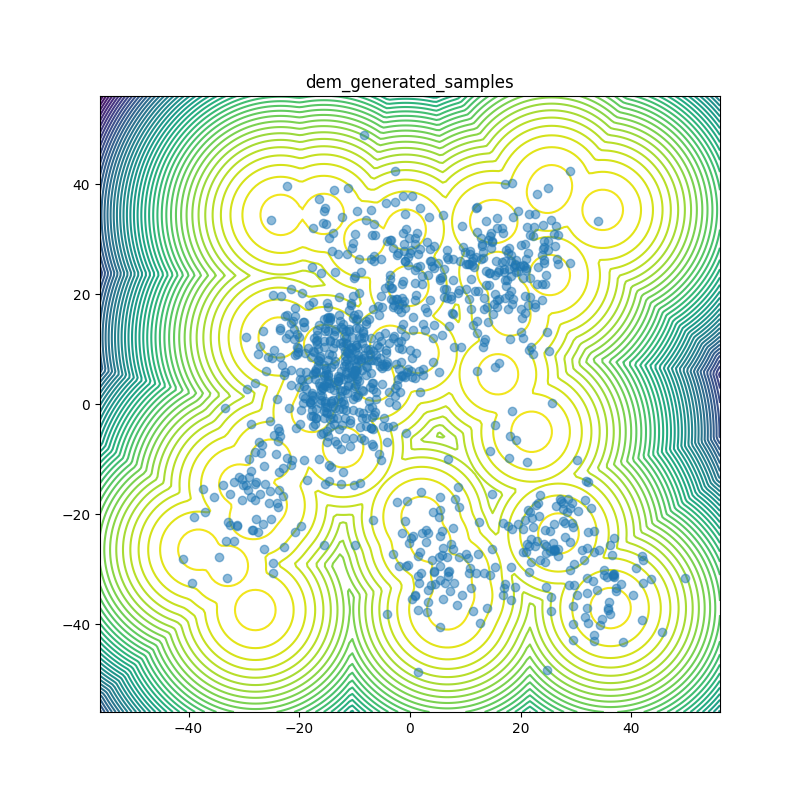
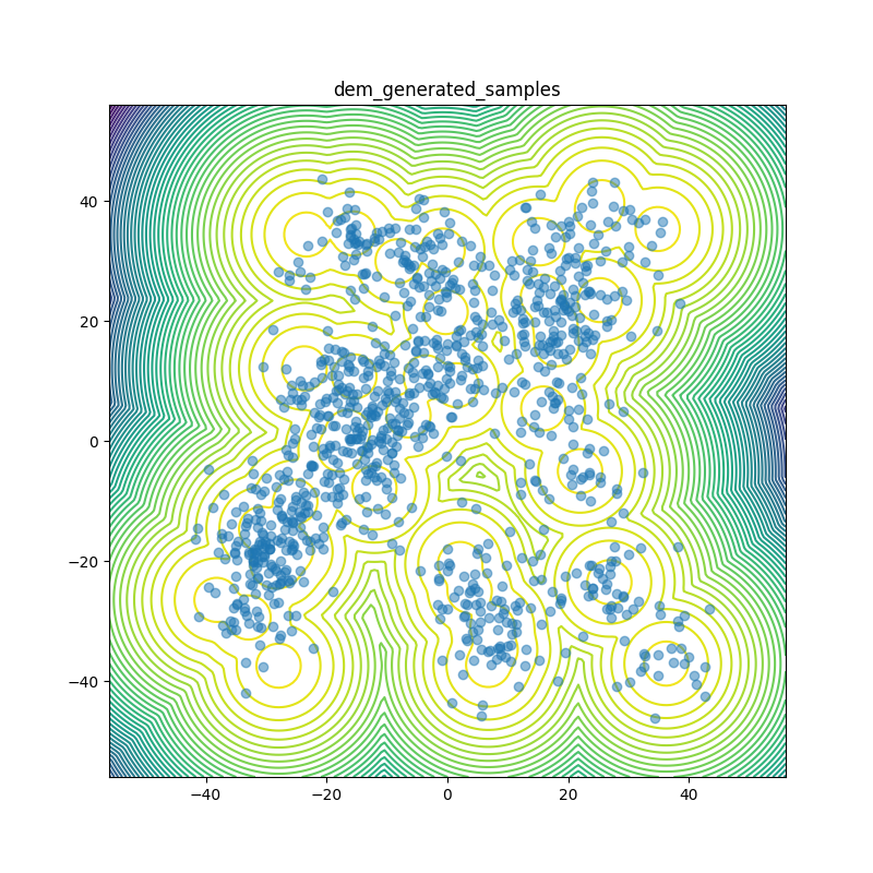
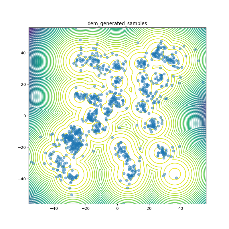
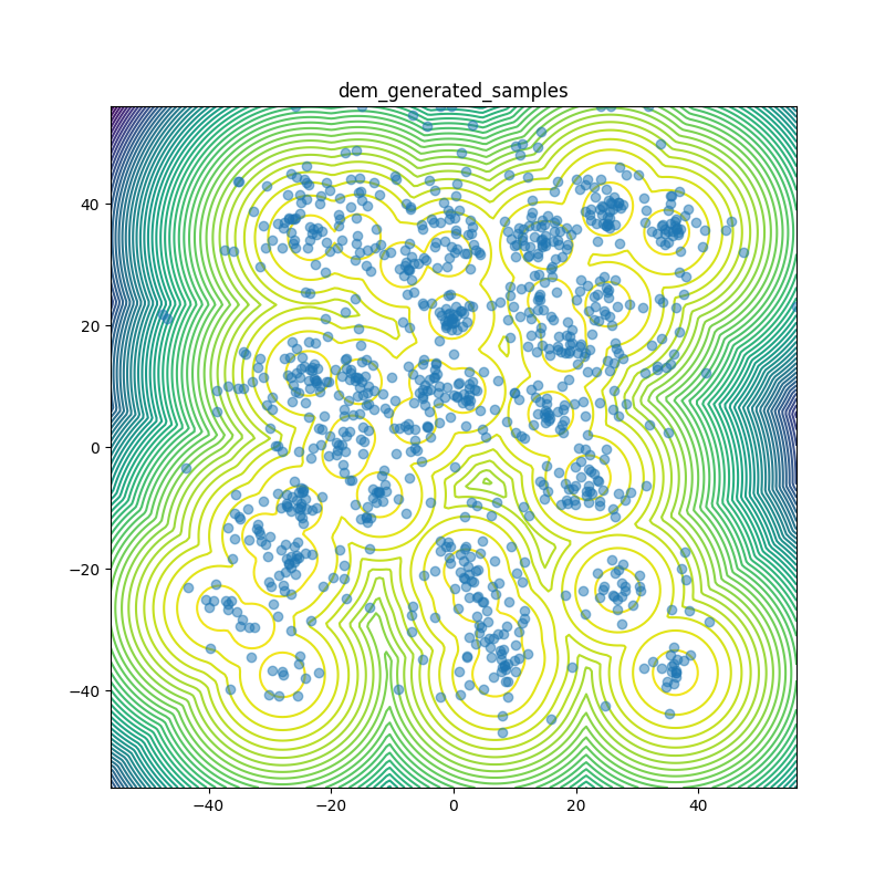
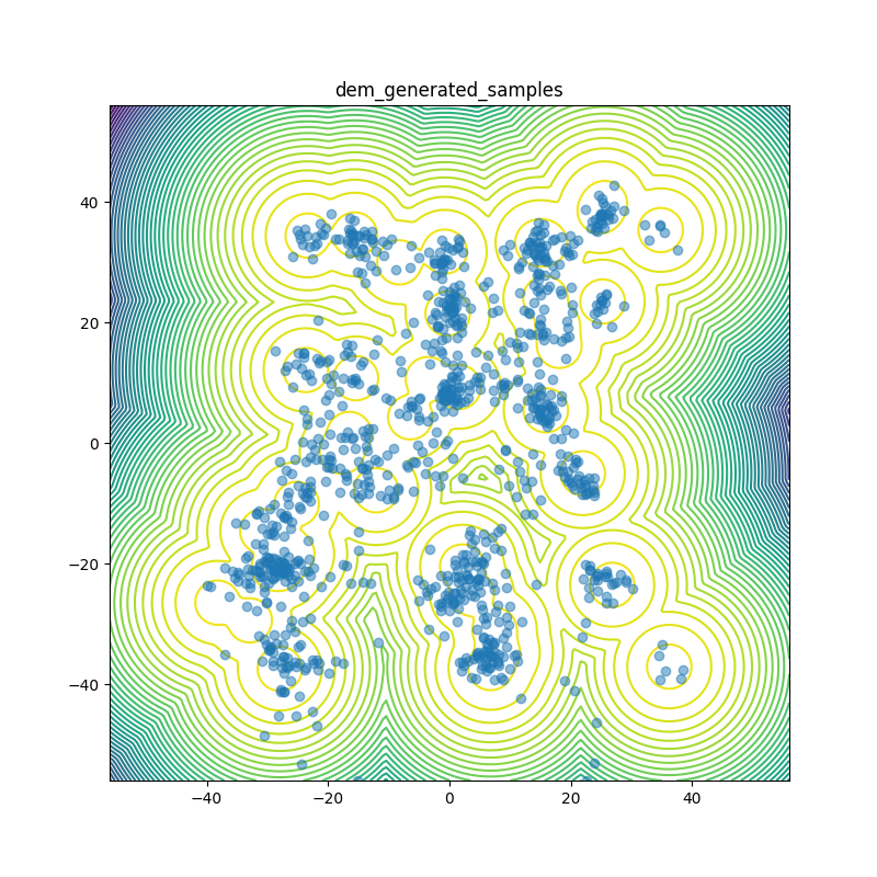
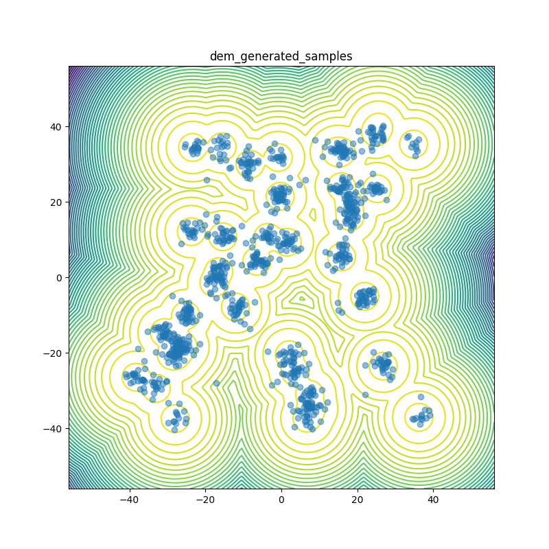
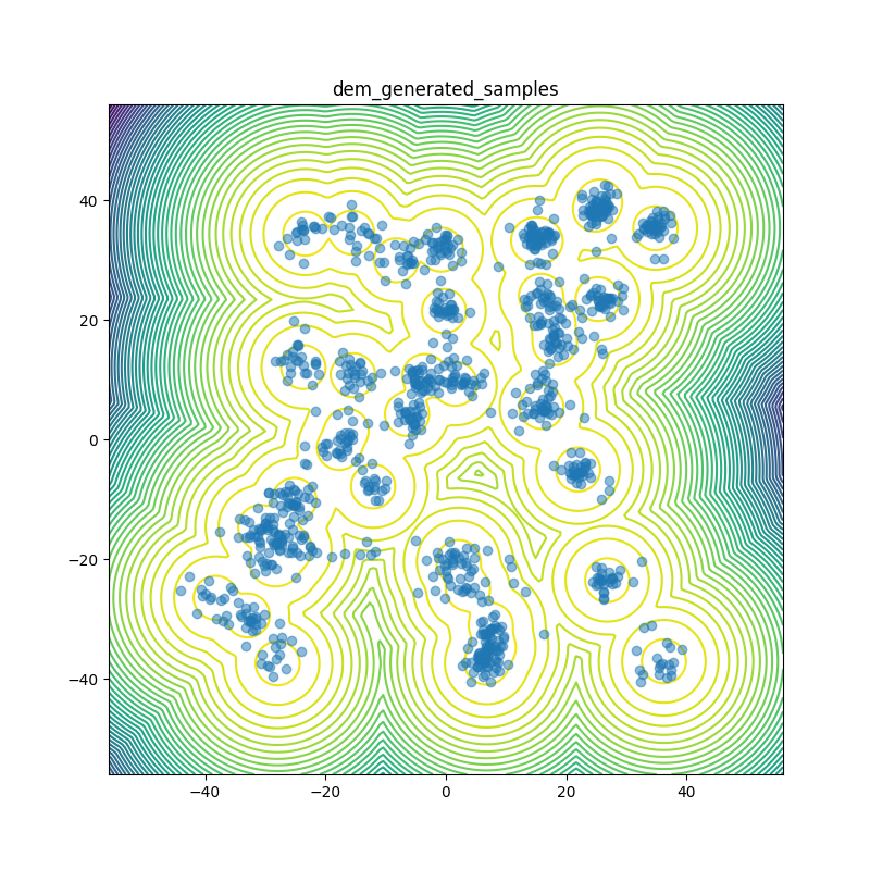
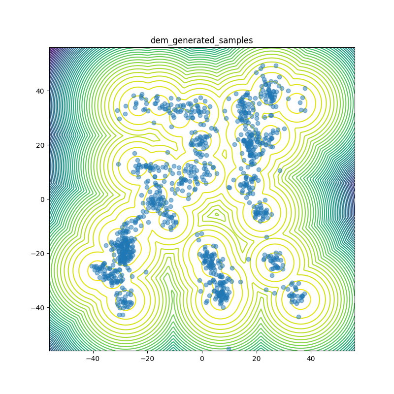
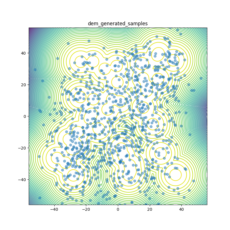
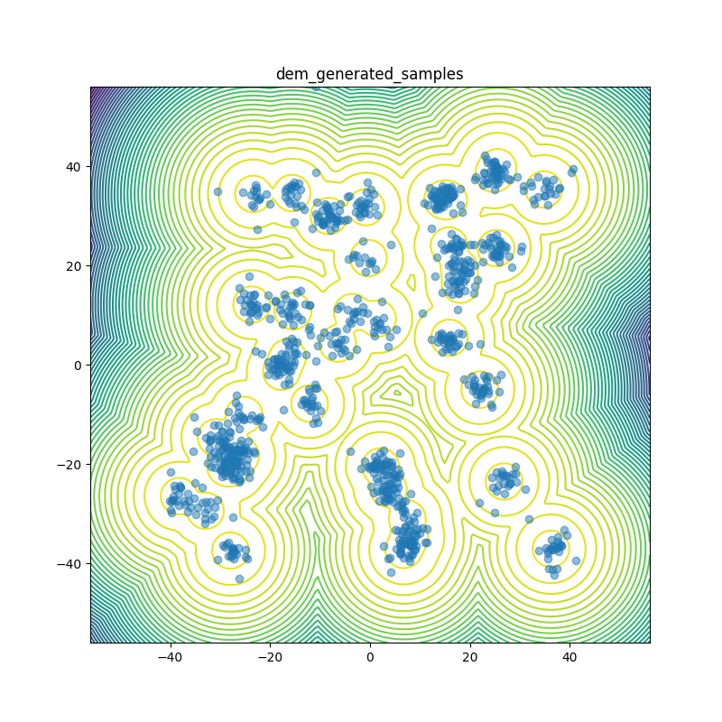
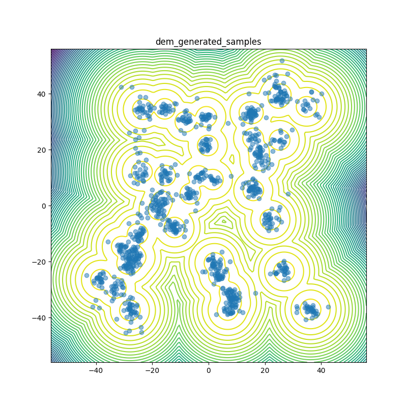
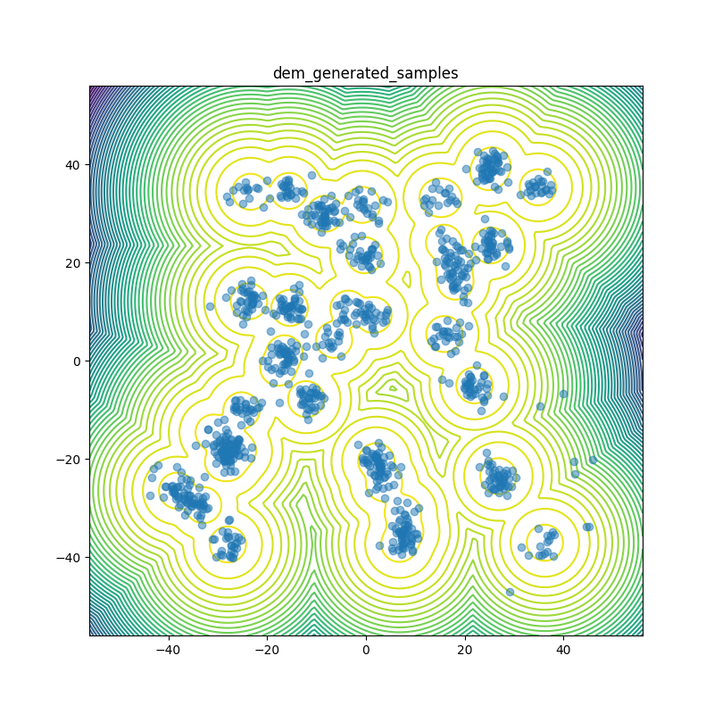
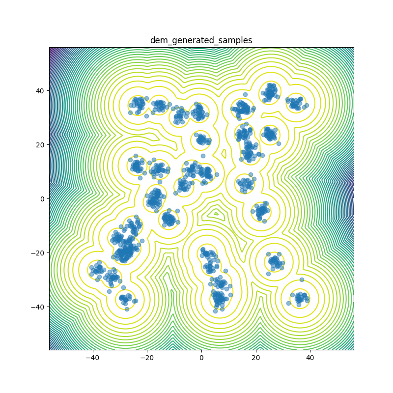
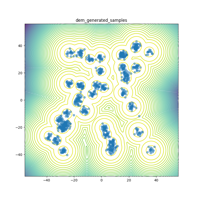
Main results. We report x-, , TV and ESS for GMM and DW-4 potentials in Table 1. It shows that when the reverse SDE integration step is limited to , EnDEM can outperform iDEM on all metrics in each task, showcasing its robustness. Furthermore, BEnDEM can outperform EnDEM by targeting the bootstrap energy estimator, achieving state-of-the-art performance. In addition, the visualized results for GMM are provided in Figure 1, which shows that EnDEM can generate samples more concentrated to the GMM modes than iDEM and BEnDEM can further boost this concentration.
5 Conclusion
In this work, we introduce EnDEM and BEnDEM, neural samplers for Boltzmann distribution and equilibrium systems like many-body systems. EnDEM uses a novel Monte Carlo energy estimator with reduced bias and variance. BEnDEM builds on EnDEM, employing an energy estimator bootstrapped from lower noise-level data, theoretically trading bias for variance. Empirically, BEnDEM achieves state-of-the-art results on the GMM and DW4 benchmarks. Future work will focus on scaling these methods to higher-dimensional tasks like Lennard-Jones potential.
Acknowledgements
José Miguel Hernández-Lobato acknowledges support from a Turing AI Fellowship under grant EP/V023756/1.
References
- Akhound-Sadegh et al., (2024) Akhound-Sadegh, T., Rector-Brooks, J., Bose, A. J., Mittal, S., Lemos, P., Liu, C.-H., Sendera, M., Ravanbakhsh, S., Gidel, G., Bengio, Y., Malkin, N., and Tong, A. (2024). Iterated denoising energy matching for sampling from boltzmann densities.
- Case et al., (2021) Case, D. A., Aktulga, H. M., Belfon, K., Ben-Shalom, I., Brozell, S. R., Cerutti, D. S., Cheatham III, T. E., Cruzeiro, V. W. D., Darden, T. A., Duke, R. E., et al. (2021). Amber 2021. University of California, San Francisco.
- Efron, (2011) Efron, B. (2011). Tweedie’s formula and selection bias. Journal of the American Statistical Association, 106(496):1602–1614.
- Flamary et al., (2021) Flamary, R., Courty, N., Gramfort, A., Alaya, M. Z., Boisbunon, A., Chambon, S., Chapel, L., Corenflos, A., Fatras, K., Fournier, N., Gautheron, L., Gayraud, N. T., Janati, H., Rakotomamonjy, A., Redko, I., Rolet, A., Schutz, A., Seguy, V., Sutherland, D. J., Tavenard, R., Tong, A., and Vayer, T. (2021). Pot: Python optimal transport. Journal of Machine Learning Research, 22(78):1–8.
- Ho et al., (2020) Ho, J., Jain, A., and Abbeel, P. (2020). Denoising diffusion probabilistic models. Advances in neural information processing systems, 33:6840–6851.
- Karras et al., (2022) Karras, T., Aittala, M., Aila, T., and Laine, S. (2022). Elucidating the design space of diffusion-based generative models. Advances in neural information processing systems, 35:26565–26577.
- (7) Klein, L., Krämer, A., and Noe, F. (2023a). Equivariant flow matching. In Oh, A., Naumann, T., Globerson, A., Saenko, K., Hardt, M., and Levine, S., editors, Advances in Neural Information Processing Systems, volume 36, pages 59886–59910. Curran Associates, Inc.
- (8) Klein, L., Krämer, A., and Noé, F. (2023b). Equivariant flow matching.
- Köhler et al., (2020) Köhler, J., Klein, L., and Noe, F. (2020). Equivariant flows: Exact likelihood generative learning for symmetric densities. In III, H. D. and Singh, A., editors, Proceedings of the 37th International Conference on Machine Learning, volume 119 of Proceedings of Machine Learning Research, pages 5361–5370. PMLR.
- Komanduri et al., (2000) Komanduri, R., Chandrasekaran, N., and Raff, L. (2000). Md simulation of nanometric cutting of single crystal aluminum–effect of crystal orientation and direction of cutting. Wear, 242(1-2):60–88.
- Leimkuhler and Matthews, (2012) Leimkuhler, B. and Matthews, C. (2012). Rational construction of stochastic numerical methods for molecular sampling. Applied Mathematics Research eXpress.
- Lyman and Zuckerman, (2007) Lyman, E. and Zuckerman, D. M. (2007). Annealed importance sampling of peptides. The Journal of chemical physics, 127(6).
- Midgley et al., (2023) Midgley, L. I., Stimper, V., Simm, G. N. C., Schölkopf, B., and Hernández-Lobato, J. M. (2023). Flow annealed importance sampling bootstrap.
- Moore et al., (2024) Moore, J. H., Cole, D. J., and Csanyi, G. (2024). Computing hydration free energies of small molecules with first principles accuracy.
- Noé et al., (2019) Noé, F., Olsson, S., Köhler, J., and Wu, H. (2019). Boltzmann generators – sampling equilibrium states of many-body systems with deep learning.
- Owen, (2023) Owen, A. B. (2023). Practical Quasi-Monte Carlo Integration. https://artowen.su.domains/mc/practicalqmc.pdf.
- Śledź and Caflisch, (2018) Śledź, P. and Caflisch, A. (2018). Protein structure-based drug design: from docking to molecular dynamics. Current opinion in structural biology, 48:93–102.
- Song and Ermon, (2019) Song, Y. and Ermon, S. (2019). Generative modeling by estimating gradients of the data distribution. Advances in neural information processing systems, 32.
- Song et al., (2020) Song, Y., Sohl-Dickstein, J., Kingma, D. P., Kumar, A., Ermon, S., and Poole, B. (2020). Score-based generative modeling through stochastic differential equations. arXiv preprint arXiv:2011.13456.
- Tong et al., (2024) Tong, A., Fatras, K., Malkin, N., Huguet, G., Zhang, Y., Rector-Brooks, J., Wolf, G., and Bengio, Y. (2024). Improving and generalizing flow-based generative models with minibatch optimal transport.
- Vargas et al., (2023) Vargas, F., Grathwohl, W., and Doucet, A. (2023). Denoising diffusion samplers.
- Woo and Ahn, (2024) Woo, D. and Ahn, S. (2024). Iterated energy-based flow matching for sampling from boltzmann densities.
- Zhang and Chen, (2022) Zhang, Q. and Chen, Y. (2022). Path integral sampler: a stochastic control approach for sampling.
- Zheng et al., (2024) Zheng, S., He, J., Liu, C., Shi, Y., Lu, Z., Feng, W., Ju, F., Wang, J., Zhu, J., Min, Y., et al. (2024). Predicting equilibrium distributions for molecular systems with deep learning. Nature Machine Intelligence, pages 1–10.
Appendix A Training Details
Algorithm 1 describes EnDEM in detail. The key difference in training the BEnDEM is only in the inner-loop.
To train the BEnDEM, it’s crucial that the bootstrap energy estimation at can be accurate only when the noised energy at is well-learned. Therefore, we need to sequentially learn energy at small t using the original MC energy estimator then refines the estimator using bootstrap for large t, which is inefficient. To be more efficient, we adapt a rejection training scheme: (a) given and , we first compute the loss of targeting the MC energy estimator (4), and ; (b) These losses indicate how does the energy network fit the noised energies at different times, and therefore compute as an indicator; (c) with probability , we accept targeting a energy estimator bootstrapped from and otherwise we stick to target the original MC estimator. We provide a full description of the inner-loop of BEnDEM training in Algorithm 2.
Appendix B Proof of Proposition 1
Proposition 1
If is sub-Gaussian, then there exists a constant such that with probability (over ) we have
| (10) |
with , where .
Proof. We first introduce the error bound of the MC score estimator , where , proposed by Akhound-Sadegh et al., (2024) as follows
| (11) |
which assumes that is sub-Gaussian. Let’s define the following variables
| (12) | ||||
| (13) |
By the sub-Gaussianess assumption, it’s easy to show that the constant term in Equation 11 is . Notice that is a logarithm of an unbiased estimator . By the sub-Gaussian assumption, one can derive that is also sub-Gaussian. Furthermore, it’s mean and variance can be derived by employing a first-order Taylor expansion:
| (14) | ||||
| (15) |
And one can obtain its concentration inequality by incorporating the sub-Gaussianess
| (16) |
By using the above Inequality 16 and the triangle inequality
| (17) | ||||
| (18) | ||||
| (19) | ||||
| (20) | ||||
| (21) |
Therefore, we have . It demonstrates a less biased estimator, which, what’s more, doesn’t require a sub-Gaussianess assumption over .
Appendix C Proof of Proposition 2
Proposition 2
If is sub-Gaussian and is bounded, the total variance of the MC score estimator is consistently larger than that of the MC energy estimator in low-energy regions, with
| (22) |
Under certain assumption, we can extend that holds on high-energy regions.
Proof. We split the proof into two parts: low-energy region and high-energy one. The proof in the low-energy region requires only the aforementioned sub-Gaussianess and bounded assumptions, while the one in the high-energy region requires an additional constraint which will be clarified later. Review that can be expressed as an importance-weighted estimator as follows:
| (23) |
Let , where . Since a bounded variable is sub-Gaussian, this assumption resembles a sub-Gaussianess assumption of . Then each element of , i.e. , is bounded by . And therefore are sub-Gaussian.
In low-energy regions. is concentrated away from as is small. Then, there exists a constant such that and thus for each element :
| (24) | ||||
| (25) |
therefore, the element of , i.e., is bounded by , suggesting it is sub-Gaussian. While Inequality 11 can be expressed as
| (26) |
We can roughly derive a bound elementwisely
| (27) |
which suggests that we can approximate the variance of by leveraging its sub-Gaussianess
| (28) |
Therefore, according to Equation 15 we can derive that
| (29) | ||||
| (30) | ||||
| (31) |
In high-energy region. we assume that there exists a direction with a large norm pointing to low energy regions, i.e. such that are positively related to . According to Section 9.2 in Owen, (2023), the asymptotic variance of a self-normalized importance sampling estimator is given by:
| (32) | ||||
| (33) | ||||
| (34) |
By substituting , , , , and , as well as using and are positive related, we have:
| (35) | ||||
| (36) |
Therefore, if we further have a large variance over the system score at this region, i.e. , then we have
| (38) |
and thus holds.
Appendix D Proof of Proposition 3
Proposition 3
Given a bootstrap trajectory such that , where , and is a small number. Suppose is converged to the estimator in Eq. 4 at . Let and , where . The variance of the bootstrap energy estimator is given by
| (39) |
and the bias of learning is given by
| (40) |
Proof. The variance of can be simply derived by leveraging the variance of a sub-Gaussian random variable similar to Equation 15. While the entire proof for bias of is organized as follows:
-
1.
we first show the bias of Bootstrap() estimator, which is bootstrapped from the system energy
-
2.
we then show the bias of Bootstrap() estimator, which is bootstrapped from a lower level noise convolved energy recursively, by induction.
D.1 Bootstrap() estimator
The Sequential estimator and Bootstrap() estimator are defined by:
| (41) | ||||
| (42) | ||||
| (43) |
The mean and variance of a Sequential estimator can be derived by considering it as the MC estimator with samples:
| (44) |
While an optimal network obtained by targeting the original MC energy estimator 4 at is 111We consider minimizing the -norm, i.e. . Since the target, , is noisy, the optimal outputs are given by the expectation, i.e. . :
| (45) |
Then the optimal Bootstrap() estimator can be expressed as:
| (46) |
Before linking the Bootstrap estimator and the Sequential one, we provide the following approximation which is useful. Let , two random variables and , are corresponding samples. Assume that are close to and concentrated at , while are concentrated at , then
| (47) | ||||
| (48) | ||||
| (49) | ||||
| (50) | ||||
| (51) | ||||
| (52) |
where Approximation applies a first order Taylor expansion of around since are close to ; while Approximation uses under the same assumption. Notice that when is large and is small , are close to and concentrated at . Therefore, by plugging them into Equation 52, Equation 46 can be approximated by
| (53) |
When is large and is small, the bias and variance of are small, then we have
| (54) |
Therefore, the optimal Bootstrap estimator can be approximated as follows:
| (55) |
where its mean and variance depend on those of the Sequential estimator (44):
| (56) | ||||
| (57) |
D.2 Bootstrap() estimator
Given a bootstrap trajectory where and , and is well learned at . Let the energy network be optimal for by learning a sequence of Bootstrap() energy estimators (). Then the optimal value of is given by . We are going to show the variance of a Bootstrap() estimator by induction. Suppose we have:
| (58) |
Then for any , the learning target of is bootstrapped from ,
| (59) | ||||
| (60) |
Assume that is small and is large, then we can apply Approximation 52 and have
| (61) |
In Bootstrap() setting, is not small and we can’t approximate simply by a MC estimator . However, we can sequentially estimate such energy by bootstrapping through the trajectory , resembling a Sequential() estimator which is equivalent to ,
| (62) |
therefore, the optimal output of the energy network at by learning this Bootstrap() estimator is
| (63) |
which suggests that the accumulated bias of a Bootstrap() estimator is given by
| (64) |
Appendix E Incorporating Symmetry Using EnDEM
We consider applying EnDEM and BEnDEM in physical systems with symmetry constraints like -body system. We prove that our MC energy estimator is -invariant under certain conditions, given in the following Proposition.
Proposition 4
Let be the product group and be a -invariant density in . Then the Monte Carlo energy estimator of is -invariant if the sampling distribution is -invariant, i.e.,
Proof. Since is -invariant, then is -invariant as well. Let acts on where . Since is equivalent to . Then we have
| (65) | ||||
| (66) | ||||
| (67) |
Therefore, is invariant to .
Furthermore, is obtained by applying a learned energy network, which is -invariant, to the analogous process and therefore is -invariant as well.
Appendix F EnDEM for General SDEs
Diffusion models can be generalized to any SDEs as , where and is a Brownian motion. Particularly, we consider , i.e.
| (68) |
Then the marginal of the above SDE can be analytically derived as:
| (69) |
where . For example, when and , where is a monotonic function (e.g. linear) increasing from to , the above SDE resembles a Variance Preserving (VP) process (Song et al.,, 2020). In DMs, VP can be a favor since it constrains the magnitude of noisy data across ; while a VE process doesn’t, and the magnitude of data can explode as the noise explodes. Therefore, we aim to discover whether any SDEs rather than VE can be better by generalizing EnDEM and DEM to general SDEs.
In this work, we provide a solution for general SDEs (68) rather than a VE SDE. For simplification, we exchangeably use and . Given a SDE as Equation 68 for any integrable functions and , we can first derive its marginal as Equation 69, which can be expressed as:
| (70) |
Therefore, by defining we have and therefore:
| (71) |
which resembles a VE SDE with noise schedule . In fact, we can also derive this by changing variables:
| (72) | ||||
| (73) | ||||
| (74) |
which also leads to Equation 71. Let be the marginal distribution of and the marginal distribution of , with we have
| (75) | ||||
| (76) | ||||
| (77) |
Therefore, we can learn scores and energies of simply by following DEM and EnDEM for VE SDEs. Then for sampling, we can simulate the reverse SDE of and eventually, we have .
Instead, we can also learn energies and scores of . By changing the variable, we can have
| (78) | ||||
| (79) |
which provides us the energy and score estimator for :
| (80) | ||||
| (81) | ||||
| (82) |
Typically, is a non-negative function, resulting in decreasing from and can be close to when is large. Therefore, the above equations realize that even though both the energies and scores for a general SDE can be estimated, the estimators are not reliable at large since can be extremely large; while the SDE of (74) indicates that this equivalent VE SDE is scaled by , resulting that the variance of at large can be extremely large and requires much more MC samples for a reliable estimator. This issue can be a bottleneck of generalizing DEM, EnDEM, and BEnDEM to other SDE settings, therefore developing more reliable estimators for both scores and energies is of interest in future work.
Appendix G Linking iDEM and iEFM Through Tweedie’s Formula
In this supplementary work, we propose TWEEdie DEM (TweeDEM), by leveraging the Tweedie’s formula (Efron,, 2011) into DEM, i.e. . Surprisingly, TweeDEM can be equivalent to the iEFM-VE proposed by Woo and Ahn, (2024), which is a variant of iDEM corresponding to another family of generative model, flow matching.
We first derive an MC estimator denoiser, i.e. the expected clean data given a noised data at
| (83) | ||||
| (84) | ||||
| (85) |
where the numerator can be estimated by an MC estimator and the denominator can be estimated by another similar MC estimator , suggesting we can approximate this denoiser through self-normalized importance sampling as follows
| (86) | ||||
| (87) |
where , are the importance weights and . Then a new MC score estimator can be constructed by plugging the denoiser estimator into Tweedie’s formula
| (88) |
where resembles the vector fields in Flow Matching. In another perspective, these vector fields can be seen as scores of Gaussian, i.e. , and therefore is an importance-weighted sum of Gaussian scores while can be expressed as an importance-weighted sum of system scores . In addition, Karras et al., (2022) demonstrates that in Denoising Diffusion Models, the optimal scores are an importance-weighted sum of Gaussian scores, while these importance weights are given by the corresponding Gaussian density, i.e. and . We summarize these three different score estimators as follows:
DEM, sum of system scores, weighted by system energies:
DDM, sum of perturbation kernel scores, weighted by perturbation densities:
EFM-VE=DEM+Tweedie, sum of perturbation kernel scores, weighted by system energies:
Appendix H Additional Experimental Details
H.1 Energy functions
GMM. A Gaussian Mixture density in -dimensional space with modes, which is proposed by Midgley et al., (2023). Each mode in this density is evenly weighted, with identical covariances,
| (89) |
and the means are uniformly sampled from , i.e.
| (90) |
Then its energy is defined by the negative-log-likelihood, i.e.
| (91) |
For evaluation, we sample data from this GMM with following Midgley et al., (2023); Akhound-Sadegh et al., (2024) as a test set.
DW-4. First introduced by Köhler et al., (2020), the DW-4 dataset describes a system with particles in -dimensional space, resulting in a task with dimensionality . The energy of the system is given by the double-well potential based on pairwise Euclidean distances of the particles,
| (92) |
where , , and are chosen design parameters of the system, the dimensionless temperature and are Euclidean distance between two particles. Following Akhound-Sadegh et al., (2024), we set , , and , and we use validation and test set from the MCMC samples in Klein et al., 2023a as the “Ground truth” samples for evaluating.
LJ-n. This dataset describes a system consisting of particles in -dimensional space, resulting in a task with dimensionality . Following Akhound-Sadegh et al., (2024), the energy of the system is given by with the Lennard-Jones potential
| (93) | ||||
| and the harmonic potential | ||||
| (94) | ||||
where are Euclidean distance between two particles, , and are physical constants, refers to the center of mass of the system and the oscillator scale. We use , , and the same as Akhound-Sadegh et al., (2024). We test our models in LJ-13 and LJ-55, which correspond to and respectively. And we use the MCMC samples given by Klein et al., 2023a as a test set.
H.2 Evaluation Metrics
2-Wasserstein distance . Given empirical samples from the sampler and ground truth samples , the 2-Wasserstein distance is defined as:
| (95) |
where is the transport plan with marginals constrained to and respectively. Following Akhound-Sadegh et al., (2024), we use the Hungarian algorithm as implemented in the Python optimal transport package (POT) (Flamary et al.,, 2021) to solve this optimization for discrete samples with the Euclidean distance . is based on the data and is based on the corresponding energy.
Effective Sample Size (ESS). This metric measures the quality and efficiency of a set of weighted samples. It quantifies the number of independent and identically distributed (i.i.d.) samples that would be needed to achieve the same level of estimation accuracy as the weighted samples. ESS is defined as
| (96) |
where and . And we follow the setting used by Akhound-Sadegh et al., (2024), which computes from a continuous normalizing flow (CNF) model and is shown to be a relatively good estimator. The CNF is trained by an optimal transport flow matching on samples from each model (OT-CFM) (Tong et al.,, 2024). Under this setting, we can compare the sample quality of various model architectures fairly using the same model architecture, training regime, and numerical likelihood approximation independent of the sampler form. Then given a test sample , its likelihood can be estimated as
| (97) |
where and the flow function.
Total Variation (TV). The total variation measures the dissimilarity between two probability distributions. It quantifies the maximum difference between the probabilities assigned to the same event by two distributions, thereby providing a sense of how distinguishable the distributions are. Given two distribution and , with densities and , over the same sample space , the TV distance is defined as
| (98) |
Following Akhound-Sadegh et al., (2024), for low-dimentional datasets like GMM, we use bins in each dimension. For larger equivariant datasets, the total variation distance is computed over the distribution of the interatomic distances of the particles.
H.3 Experiment Settings
We set the reverse SDE integration steps for iDEM, EnDEM, and BEnDEM in our main experiment as . In experiments for TweeDEM, we set this integration step for TweeDEM and iDEM.
GMM-40. For the basic model , we use an MLP with sinusoidal and positional embeddings which has layers of size as well as positional embeddings of size . The replay buffer is set to a maximum length of .
During training, the generated data was in the range so to calculate the energy it was scaled appropriately by unnormalizing by a factor of . All models are trained with a geometric noise schedule with , , samples for computing both the MC score estimator and MC energy estimator , samples for computing the Bootstrap energy estimator and Bootstrap score estimator and we clipped the norm of and to . All models are trained with a learning rate of .
DW-4. All models use an EGNN with message-passing layers and a -hidden layer MLP of size . All models are trained with a geometric noise schedule with , , a learning rate of , samples for computing and , samples for computing and , and we clipped and to a max norm of .
LJ-13. All models use an EGNN with hidden layers and hidden layer size . All models are trained with a geometric noise schedule with and , a learning rate of , samples for and , samples for and , and we clipped and to a max norm of .
For all datasets. We use clipped scores as targets for iDEM and TweeDEM training for all tasks. Meanwhile, we also clip scores during sampling in outer-loop of training, when calculating the reverse SDE integral. These settings are shown to be crucial especially when the energy landscape is non-smooth and exists extremely large energies or scores, like LJ-13 and LJ-55. In fact, targeting the clipped scores refers to learning scores of smoothed energies. While we’re learning unadjusted energy for EnDEM and BEnDEM, the training can be unstable, and therefore we blue smooth the Lennard-Jones potential through the cubic spline interpolation, according to Moore et al., (2024). Besides, we predict per-particle energies for LJ-n datasets. It shows that this setting can significantly stabilize training and boost performance.
Appendix I Supplementary Experients
I.1 Comparing the Robustness of Energy-Matching and Score-Matching
In this section, we discussed the robustness of the energy-matching model(EnDEM) with the score-matching model(iDEM) by analyzing the influence of the numbers of MC samples used for estimators and choice of noise schedule on the sampler’s performance.
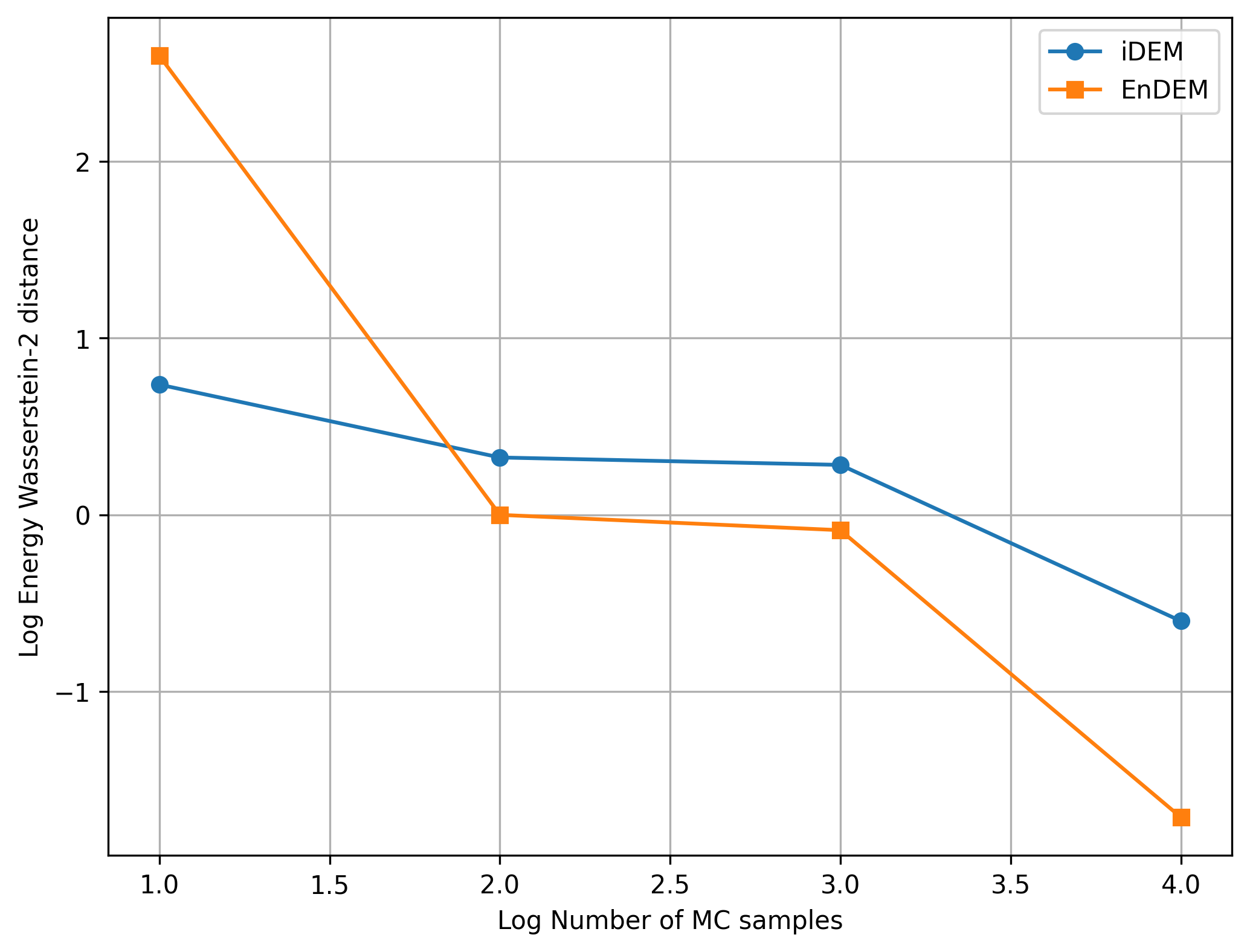
As in Figure 2, EnDEM consistently outperforms iDEM when more than 100 MC samples are used for the estimator. Besides, Endem shows a faster decline when the number of MC samples increases. Therefore, we can conclude that the low variance of Energy-matching makes it more beneficial when we boost with more MC samples.


Then, we evaluate the performance differences when applying various noise schedules. The following four schedules were tested in the experiment:
-
•
Geometric noise schedule: The noise level decreases geometrically in this schedule. The noise at step is given by: where is the initial noise level, is the maximum noise level, and is the time step.
-
•
Cosine noise schedule: The noise level follows a cosine function over time, represented by: , where is a hyper-parameter that controls the decay rate.
-
•
Quadratic noise schedule: The noise level follows a quadratic decay: where is the initial noise level. This schedule applies a slow decay initially, followed by a more rapid reduction.
-
•
Linear noise schedule: In this case, the noise decreases linearly over time, represented as:
The experimental results are depicted in Figure 3 and Figure 4. It is pretty obvious that for iDEM the performance varied for different noise schedules. iDEM favors noise schedules that decay more rapidly to when approaches 0. When applying the linear noise schedules, the samples are a lot more noisy than other schedules. This also proves our theoretical analysis that the variance would make the score network hard to train. On the contrary, all 4 schedules are able to perform well on EnDEM. This illustrates that the reduced variance makes EnDEM more robust and requires less hyperparameter tuning.
I.2 Scaling up to Lennard Jones Potential
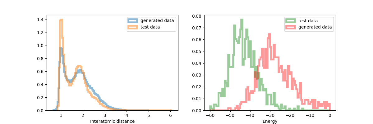
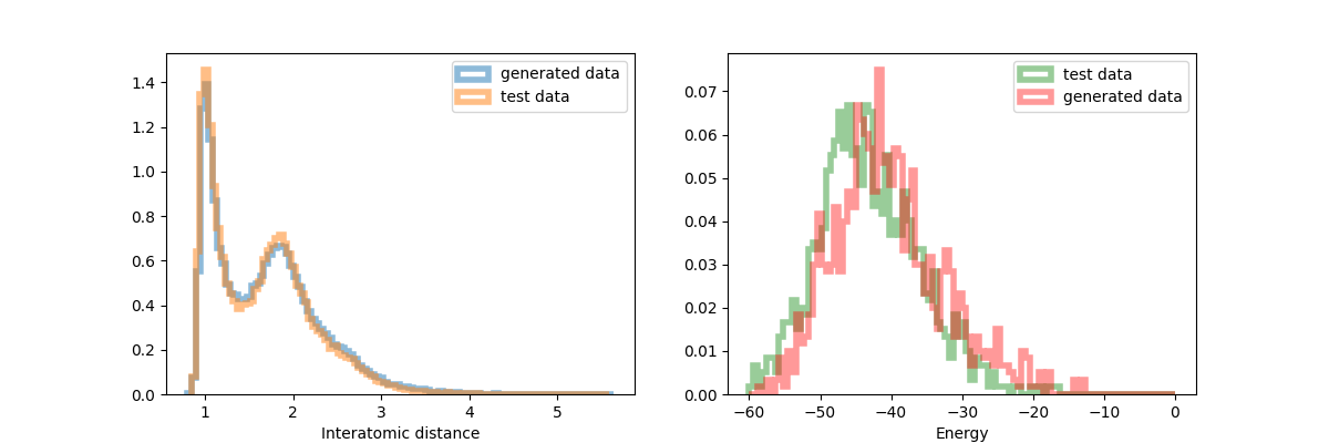
Besides GMM and DW-4, we would also like to show preliminary experimental results on the LJ-13 potentials. The distributions of interatomic distances and energies are shown in Figure 5.
The performance comparison between iDEM and EnDEM for the LJ-13 potential demonstrates the superior accuracy of EnDEM in capturing both the interatomic distance distribution and energy distribution. These results suggest that EnDEM’s capabilities allow it to generalize better in complex many-body systems, like the Lennard-Jones potential, providing more reliable energy estimations and physical interpretations.
I.3 Empirical Analysis of the Variance of and
To justify the theoretical results for the variance of the MC energy estimator (4) and MC score estimator (2), we first empirically explore a D GMM. For better visualization, the GMM is set to be evenly weighted by modes located in with identical variance for each component, resulting in the following density
| (99) |
while the marginal perturbed distribution at can be analytically derived from Gaussian’s property:
| (100) |
given a VE noising process.
We empirically estimate the variance for each pair of by simulating times the MC estimators. Besides, we estimate the expected variance over for each time , i.e. and .

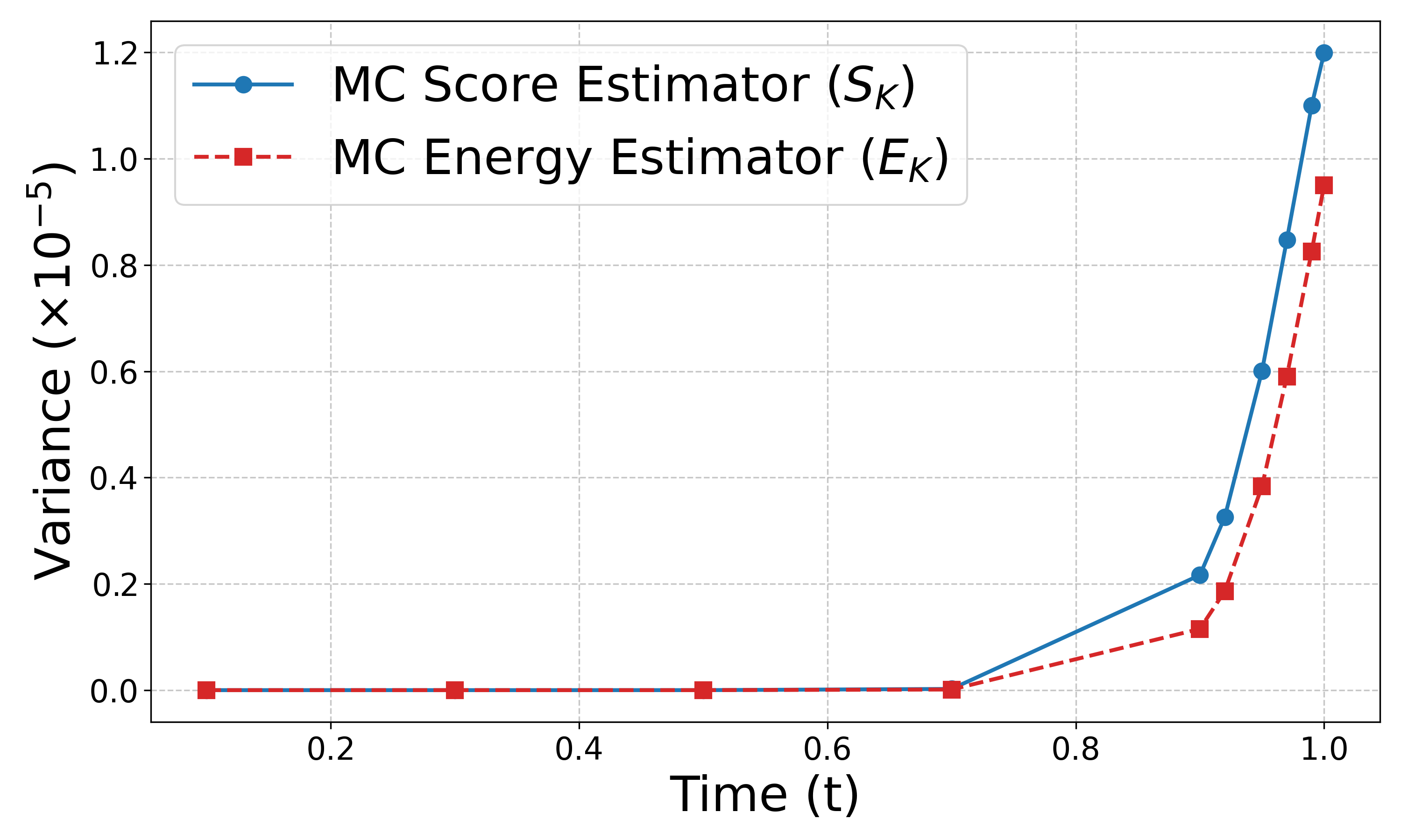
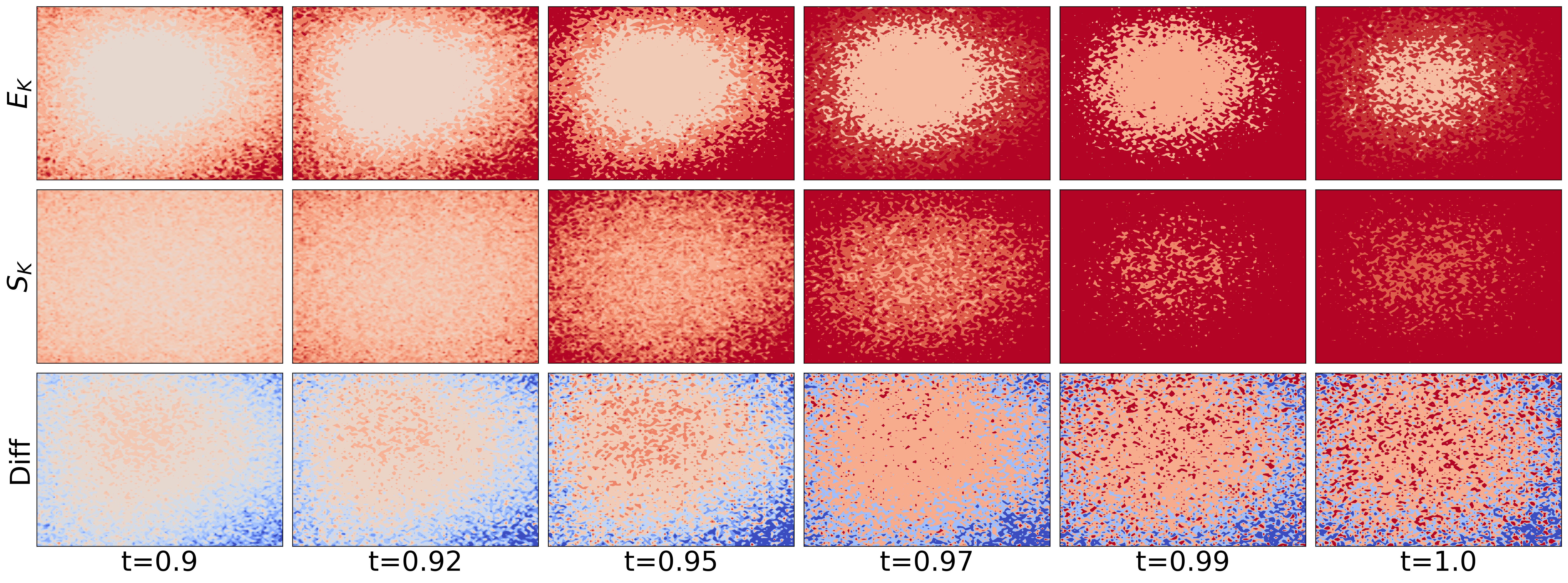
Figure 6(a) shows that, the variance of both MC energy estimator and MC score estimator increase as time increases. In contrast, the variance of can be smaller than that of in most areas, especially when the energies are low (see Figure 6(c)), aligning our Proposition 2. Figure 6(b) shows that in expectation over true data distribution, the variance of is always smaller than that of across .
I.4 Experiments for TweeDEM

| Energy | GMM-40 () | DW-4 () | ||||||
|---|---|---|---|---|---|---|---|---|
| Sampler | x- | - | TV | ESS | x- | - | TV | ESS |
| 2.864 | 0.010 | 0.812 | 0.342 | 1.841 | 0.040 | 0.092 | 0.348 | |
| (ours) | 2.506 | 0.124 | 0.826 | 0.267 | 1.835 | 0.145 | 0.087 | 0.367 |
| iDEM | 3.98 | - | 0.81 | 0.746 | 2.09 | - | 0.09 | 0.827 |
| iDEM (rerun) | 6.406 | 46.90 | 0.859 | 0.200 | 1.862 | 0.030 | 0.093 | 0.383 |
| iEFM-VE | 4.31 | - | - | - | 2.21 | - | - | - |
| iEFM-OT | 4.21 | - | - | - | 2.07 | - | - | - |
| TweeDEM (ours) | 3.182 | 1.753 | 0.815 | 0.280 | 1.910 | 0.217 | 0.120 | 0.372 |
In Appendix G, we propose TweeDEM, a variant of DEM by leveraging Tweedie’s formula (Efron,, 2011), which theoretically links iDEM and iEFM-VE and suggests that we can simply replace the score estimator (2) with (88) to reconstruct a iEFM-VE. We conduct experiments for this variant with the aforementioned GMM and DW-4 potential functions.
Setting. We follow the ones aforementioned, but setting the steps for reverse SDE integration , the number of MC samples for GMM and for DW-4. We set a quadratic noise schedule ranging from to for TweeDEM in DW-4.
To compare the two score estimators and fundamentally, we first conduct experiments using these ground truth estimations for reverse SDE integration, i.e. samplers without learning. In addition, we consider using a neural network to approximate these estimators, i.e. iDEM and TweeDEM.
Table 2 reports x-, , TV and ESS for GMM and DW-4 potentials. We admit that we follow the instructions in the repository released by Akhound-Sadegh et al., (2024) but can’t reproduce the ESS they reported. Therefore, we rerun the iDEM and evaluate it for a more reliable comparisom. Table 2 shows that when using the ground truth estimators for sampling, there’s no significant evidence demonstrating the privilege between and . However, when training a neural sampler, TweeDEM can significantly outperform iDEM (rerun), iEFM-VE, and iEFM-OT for GMM potential. While for DW4, TweeDEM outperforms iEFM-OT and iEFM-VE in terms of but are not as good as our rerun iDEM.
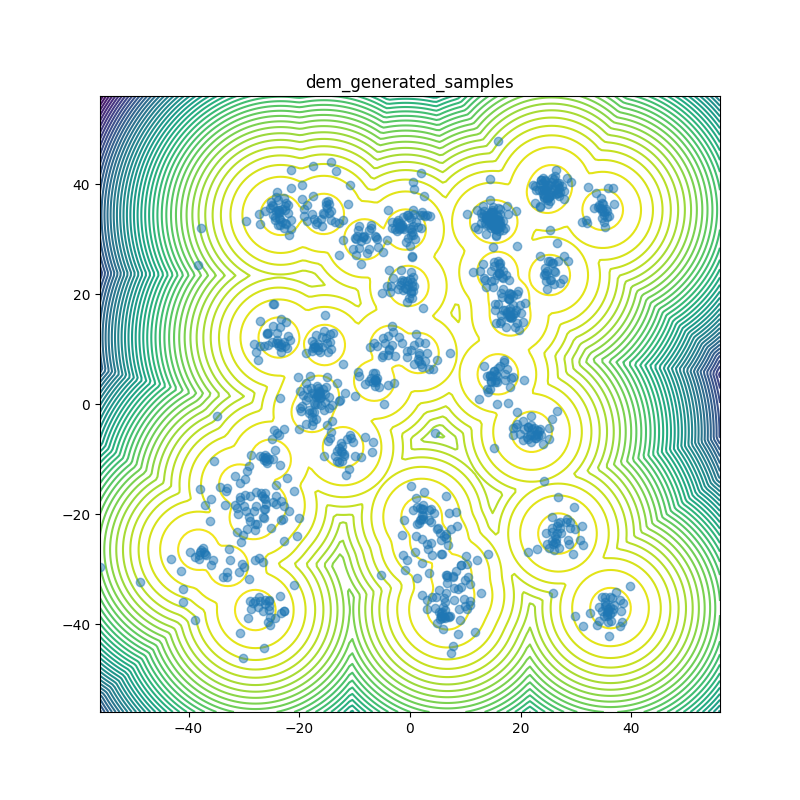
Figure 7 visualizes the generated samples from ground truth samplers, i.e. and , and neural samplers, i.e. TweeDEM and iDEM. It shows that the ground truth samplers can generate well mode-concentrated samples, as well as TweeDEM, while samples generated by iDEM are not concentrated on the modes and therefore result in the high value of based metrics. Also, this phenomenon aligns with the one reported by Woo and Ahn, (2024), where the iEFM-OT and iEFM-VE can generate samples more concentrated on the modes than iDEM.
Above all, simply replacing the score estimator with can improve generated data quality and outperform iEFM in GMM and DW-4 potentials. Though TweeDEM can outperform the previous state-of-the-art sampler iDEM on GMM, it is still not as capable as iDEM on DW-4. Except scaling up and conducting experiments on larger datasets like LJ-13, combing and is of interest in the future, which balances the system scores and Gaussian ones and can possibly provide more useful and less noisy training signals. In addition, we are considering implementing a denoiser network for TweeDEM as our future work, which might stabilize the training process.