RandALO: Out-of-sample risk estimation in no time flat
Abstract
Estimating out-of-sample risk for models trained on large high-dimensional datasets is an expensive but essential part of the machine learning process, enabling practitioners to optimally tune hyperparameters. Cross-validation (CV) serves as the de facto standard for risk estimation but poorly trades off high bias (-fold CV) for computational cost (leave-one-out CV). We propose a randomized approximate leave-one-out (RandALO) risk estimator that is not only a consistent estimator of risk in high dimensions but also less computationally expensive than -fold CV. We support our claims with extensive simulations on synthetic and real data and provide a user-friendly Python package implementing RandALO available on PyPI as randalo and at https://github.com/cvxgrp/randalo.
1 Introduction
Training machine learning models is an often expensive process, especially in large data settings. Not only is there significant cost in the fitting of individual models, but even more importantly, the best model must be chosen from a set of candidates parameterized by a set of “hyperparameters” indexing the models, and each of these models must be fitted and evaluated in order to make the optimal selection. As a result, model selection, also called hyperparameter tuning, tends to be the most computationally expensive part of the machine learning pipeline.
In order to evaluate models, we typically need to set aside unseen “holdout” data to estimate the risk of the model on new samples from the training distribution. When we have an abundance of training samples, such as in the millions or billions, we can afford to set aside a modest holdout set of tens of thousands of examples without compromising model performance. We can then simply evaluate the fitted model on the holdout set and obtain a high precision estimate of model risk, with the only major cost being the fitting of the model on the training data.
In even moderately large data regimes, however, when we have at most tens of thousands of possibly high-dimensional training samples, it is often not possible to set aside a sufficiently large holdout set without sacrificing the quality of our model fit. In these settings, the time-trusted technique for model evaluation is -fold cross-validation (CV): the data is partitioned into roughly equal subsets, and each subset is used as a holdout set while the model is trained on the remaining data, and finally the model risks across each of the folds are averaged. In this way, we get the advantage of evaluating our model on a set of data the same size as the training data.
The downsides of CV are two-fold. Firstly, for each of the folds, a new model must be fit, increasing the computational cost of evaluating risk, and thus model selection, by roughly a factor of .111The cost of training individual models on the fraction of the data is generally a bit less than the cost of training a model on the full dataset, so the total cost is a little less than times. Secondly, and perhaps more alarmingly, -fold CV provides an unbiased estimate only for the risk of a model trained on data points, which can be quite different from the risk of a model trained on points in high dimensions (Donoho et al., 2011). This bias only vanishes as approaches the number of training samples, at which point it becomes known as leave-one-out CV, at the expense of a tremendous computational cost.
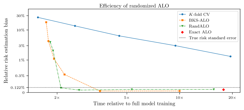
In this work, we propose a randomzied risk estimation procedure (RandALO) that addresses both of these issues. Figure 1 compares bias and real-world wall-clock time for -fold CV to our method RandALO on a high-dimensional lasso problem (experimental details in Section 5.1). Regardless of the choice of , we can implement our method with some choice of Jacobian–vector products and achieve lower bias and lower computational cost. RandALO provides very high quality risk estimates with only bias in around the time of training a model, while we would have to use and nearly the training time to achieve merely bias with -fold CV.
Our method is based on the approximate leave-one-out (ALO) technique of Rahnama Rad and Maleki (2020), which approximates leave-one-out CV using a single step of Newton’s method for each training point. This technique has been shown to enjoy the same consistency properties as leave-one-out CV for large high-dimensional datasets, thus being more accurate than -fold CV. However, a barrier to applying ALO is its poor scaling with dataset size. To address this, we employ randomized numerical linear algebra techniques to reduce the computation down to the cost of solving a constant number of quadratic programs involving the training data, which is enough to be computational advantageous against even the low cost of -fold CV with highly optimized solvers for methods such as the lasso. For non-standard and less optimized solvers, the computational advantage is even more dramatic.
We have also created a Python package, available on PyPI as randalo and at https://github.com/cvxgrp/randalo, that makes applying RandALO as simple as cross-validation. Users can use their solver of choice to first fit the model on all of the training data, and then use our package to estimate its risk. For example, for an ordinary scikit-learn (Pedregosa et al., 2011) Lasso model, we can obtain a RandALO risk estimate with a single additional line of code:
Contributions.
Concretely, our contributions are as follows:
-
1.
We develop a randomized method RandALO (Algorithm 1) for efficiently and accurately computing ALO given access to a Jacobian–vector product oracle for the fully trained model.
-
2.
We prove the asymptotic normality and decorrelation of randomized diagonal estimation for Jacobians of generalized ridge models with high-dimensional elliptical sub-exponential data (Theorem 1).
-
3.
We show that Jacobian–vector products for linear models with non-smooth regularizers can be computed efficiently via appropriate quadratic programs (Theorem 2).
-
4.
We provide extensive experiments in Section 5 demonstrating the advantage of randomized ALO over -fold CV in terms of both risk estimation and computation across a wide variety of linear models and high-dimensional synthetic and real-world datasets.
-
5.
We provide a Python software package that enables the easy application of RandALO to real-world machine learning workflows.
1.1 Related work
Risk estimation is an important aspect of model selection and has a wide literature and long history in machine learning: we refer the reader to Hastie et al. (2009), Chapter 7; Arlot and Celisse (2010); and Zhang and Yang (2015) for an overview of common techniques, particularly emphasizing cross-validation (CV). Generalized cross-validation (GCV) (Craven and Wahba, 1978) is an approximation to leave-one-out (LOO) CV that can be efficiently implemented using randomized methods (Hutchinson, 1990) and has recently been shown to be consistent for linear in high dimensions under certain random matrix assumptions (Patil et al., 2021; Bellec, 2023) and in sketched models (Patil and LeJeune, 2024).
Approximate leave-one-out (ALO) generalizes GCV by performing individual Newton steps toward the LOO objective for each training point rather than making a single uniform correction, coinciding with exact LOO for ridge regression. ALO was proposed for logistic regression (Pregibon, 1981) and kernel logistic regression (Cawley and Talbot, 2008) via iteratively reweighted least squares. More recently, Rahnama Rad and Maleki (2020) showed consistency of ALO under appropriate random data assumptions in high dimensions for arbitrary losses and regularizers (Xu et al., 2021), including non-smooth penalties such as (Auddy et al., 2024). Related and complementary to our work, Stephenson and Broderick (2020) propose to exploit the sparsity in the linear model to reduce computation in ALO. In another direction, Luo et al. (2023) share our aim in making ALO more useful by providing an extension to models obtained from iterative solvers that is consistent along the entire optimization path. Techniques based on approximate leave-one-out have also been among the most successful methods for data attribution in deep learning (Park et al., 2023).
Randomized numerical methods and risk estimation have been paired for decades, with the randomized trace estimator of Hutchinson (1990) originally proposed for estimating the degrees of freedom quantity in GCV used for correcting residuals. Bekas et al. (2007) extended Hutchinson’s approach to a method for estimating the diagonal elements of a matrix, which we base our method upon. Baston and Nakatsukasa (2022) combined this estimator with ideas from Hutch++ (Meyer et al., 2021) to create an improved estimator called Diag++ when the computational budget can be directed towards a prominent low rank component, and Epperly et al. (2024) improve this estimator by enforcing exchangeability in their method XDiag. We found both Diag++ and XDiag to be less accurate than the procedure of Bekas et al. (2007) when the number of matrix–vector products is restricted to be much below the effective rank of the matrix and so did not incorporate them into our method.
2 Approximate leave-one-out for linear models
We consider the class of linear models obtained by empirical risk minimization, having the form
| (1) |
where is an i.i.d. training data set, is a twice differentiable loss function, and is a possibly non-differentiable regularizer. In model selection, we aim to optimize the risk of the model for some risk function :
| (2) |
Here the expectation is taken over an independent sample drawn from the same distribution as the training data, as well as over the training data used to fit the model .222While in principle one would prefer the conditional risk given , cross-validation is only able to estimate marginal risk (Bates et al., 2024). Given a partition of , the cross-validation (CV) family of risk estimators have the following form:
| (3) |
The popular -fold CV consists of a partition of subsets approximately equal in size, while leave-one-out (LOO) CV uses the partition of singletons . Choosing the cross-validation partition is an accuracy–computation trade-off, as using a few large subsets (as in -fold CV) results in relatively quick but low-quality biased risk estimates, while using many small subsets (as in LOO CV) results in high-quality but computationally intensive risk estimates.
Leave-one-out risk estimation naïvely has a cost of essentially times the cost of training the model, which becomes prohibitive for moderately large . However, in certain settings, there are “shortcut” formulas that enable the efficient computation of the LOO predictions starting from the model trained on all of the data. Notably, in the setting of ridge regression where and , we have the following exact form of the LOO prediction in terms of the full prediction and the data matrix formed by stacking the data as rows:
| (4) |
The matrix is often called the “hat” matrix or linear smoothing matrix, and it is also the Jacobian matrix of predictions of the model trained on the full data with respect to the training labels , since . Computing and extracting has the same computational complexity as computing the exact full ridge solution , such as when using a Cholesky decomposition of which can be reused to compute , and so LOO CV can be performed at minimal additional cost.
Outside of ridge regression, LOO can be approximated for each data point by a single step of Netwon’s method towards minimizing the CV objective in the right-hand side of 3 starting from the full solution . This idea was proposed for logistic regression as early as Pregibon (1981), but was only recently proven to provide consistent risk estimation in high dimensions (Rahnama Rad and Maleki, 2020). For general twice differentiable losses and regularizers (note: ALO can also be applied with non-smooth regularizers, as we describe in Section 4), the approximate leave-one-out (ALO) prediction is given by
| (5) |
Here and , while . The matrix is closely related to the Jacobian via the scaling transformation , and so with some abuse of nomenclature we also refer to as the Jacobian. Note that ALO coincides exactly with LOO in the case of ridge regression. We also note that by formulating ALO in terms of the Jacobian, the corrected predictions can be computed without dependence on a specific parameterization of the prediction function. While we consider linear models for the remainder of this work, we describe in Appendix A how ALO can be derived and applied for arbitrary nonlinear prediction functions.
Although LOO and ALO have similar cost to obtaining models via direct methods such as matrix inversion, predictors in machine learning are often found by iterative algorithms that return a high-quality approximate solution very quickly. In ridge regression for example, a solution can be found in time where is the condition number of (see, e.g., Golub and Van Loan, 2013, §11.3). This can be significantly less time than the time needed to perform the inversion in the computation of using direct numerical techniques. In general, this means that it can be significantly faster to obtain a risk estimate via -fold CV which does not require computing the diagonals of , making exact ALO unattractive compared to -fold CV for large-scale data. However, by leveraging randomized methods, we can exploit the same iterative algorithms to approximate ALO in time comparable to or better than the solving for the original full predictor, yielding a risk estimate that often outperforms -fold CV in both accuracy and computational cost.
3 Randomized approximate leave-one-out
The computational bottleneck of ALO lies in extracting the diagonals of the Jacobian . Doing this exactly requires first realizing the full matrix , which is prohibitive in large data settings. This motivates our use of randomized techniques for estimating the diagonal elements of using the extension of Hutchinson’s trace estimator proposed by Bekas et al. (2007). We refer to this method as “BKS” after the names of the authors. This randomized diagonal estimate requires only Jacobian–vector products:
| (6) |
where are i.i.d. Rademacher random vectors, taking values with equal probability, and denotes the element-wise product. It is straightforward to see that and that converges to almost surely as by the strong law of large numbers. However, we need to keep small in order to minimize computation; using for example would have similar computational cost to evaluating in full.
Fortunately, for large scale machine learning problems, the number of Jacobian–vector products needed to reach a desired level of accuracy generally does not increase with the scale of the problem. We capture this formally with the following theorem under elliptical random matrix assumptions on the data, specializing to the case of generalized ridge regression with the regularizer . Note that this matches the general form of 5, aside from possible dependence of on . We prove this result for sub-exponential random data with arbitrary covariance structure and thus can expect the takeaways to be quite general.
Theorem 1.
Let for , where is a diagonal matrix with positive diagonal elements in a finite interval separated from , are i.i.d. zero-mean and unit-variance -sub-exponential variables for some , and are positive semidefinite matrices such that has eigenvalues in . Then for any and , we have the following convergence almost surely in the limit as such that ,
| (7) |
where and .
Proof sketch.
As discussed above, the BKS estimator is unbiased and so . In the case , the remainder has the form . We then apply Lyapunov’s central limit theorem over the randomness in with an appropriate argument that the terms of the sum are not too sparse. Application of the Woodbury identity allows us to extract from inside the inverse and determine the influence of , and then using random matrix theory we can argue that can be reintroduced to obtain the limiting values of and . To show uncorrelatedness, we observe that , which asymptotically vanishes due to the independence of and . We give the proof details along with the definition of -sub-exponential variables in Appendix B. ∎
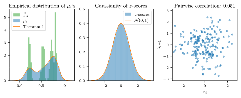
Although the statement of Theorem 1 is asymptotic in and , the distributional convergence occurs very quickly. We illustrate this on a small problem with and in Figure 2. We generate a single fixed dataset with taking values with equal probability, with equal proportion, with with equal proportion, and . Then over 1000 random trials of drawing and computing Jacobian–vector products, we examine the empirical distributions of the results. First, in the left-most plot, we compare the histogram of the ’s (200,000 values total) to the asymptotic density
| (8) |
which is the convolution of the Gaussian error distributions from Theorem 1 with the point masses at each , revealing a near-exact match. In the middle plot, we compare the histogram of -scores—that is, left-most expression in 7—another 200,000 values, with the standard normal density, but this time for only to show that Gaussianity arises without any averaging. In the right-most plot, we demonstrate the uncorrelatedness of the errors by taking the -scores of a single Jacobian–vector product and showing that successive pairs and (199 pairs total) are uncorrelated, as predicted, meaning that we can treat the errors as independent in downstream analysis.
The key takeaway for developing an efficient method for computing ALO is that since the and are even as , the variance of the ’s are regardless of problem size. Furthermore, since the noise is asymptotically uncorrelated across , it is easy to understand the effect on estimation error downstream. On the other hand, however, the quantities and also do not tend to vanish with problem size, so if we want to minimize the number of Jacobian–vector products, we must be able to handle this non-vanishing noise effectively.
3.1 Dealing with noise: Inversion sensitivity
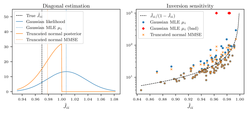
When applying ALO, each corrected prediction is an affine function of . Because of the division by , this means that ALO is extremely sensitive to noise in the estimation of . Unfortunately, by Theorem 1, we know that for any , there is always some nonzero probability that will be near or greater than 1, which means that naïvely plugging in the BKS diagonal estimate would sometimes result in extremely incorrect predictions .
It is straightforward to check that the values must lie in , so one possible solution would be to clip the values of if they are larger than to avoid near division by 0 or an incorrect sign. However, it is difficult to choose robustly: for example, as ridge regression approaches interpolating least squares in high dimensions, the values of approach 1, so a non-adaptive value of would give an inconsistent result. A more sophisticated approach would be to perform minimum mean squared error (MMSE) estimation of given the individual diagonal estimates and an appropriate prior on supported on . Since these diagonal estimates are uncorrelated Gaussian variables by Theorem 1, the sufficient statistics for this estimation problem are the sample means and the sample variances
| (9) |
If we assume that ’s are sufficiently well estimated to plug in in place of the true variances, we can compute the posterior distribution of given and for a uniform prior on :
| (10) |
Thus, the MMSE estimator is the conditional mean of this distribution, which is the mean of a truncated normal distribution with location and scale parameters and on the interval . Numerical functions for evaluating this mean are commonly available in standard scientific computing packages, making this estimator computationally efficient and trivial to implement. We demonstrate the effectiveness of this approach in Figure 3, and we refer to the method in which we plug in the MMSE estimates of into 5 and use the resulting to evaluate risk as BKS-ALO.
This simple MMSE estimation approach enables us to gracefully handle noise that would otherwise need to be handled downstream in the algorithm using ad hoc outlier detection. Furthermore, it still has asymptotic normality in , matching the distribution of , and so makes it straightforward to reason about the remaining bias introduced by noisy estimation of diagonals in ALO.
3.2 Dealing with noise: Risk inflation debiasing
Since the variances of decay only at a rate of , the effects of estimation noise will appear in our risk estimate for any finite . Unfortunately, as demonstrated in Figure 3 (right), the noise can be substantial even for moderate numbers of Jacobian–vector products such as . The effect of this noise is typically a bias towards an inflated estimate of risk, larger than the true risk. To see why this is generally the case, consider a sufficiently large such that Gaussianity is preserved through the mapping and thus for some ,
| (11) |
Let be the ALO-corrected prediction evaluated at instead of , such that for independent of , , and . Now consider any convex risk function . By the law of large numbers and Jensen’s inequality, we should expect to see bias for large . Letting , , and denote random variables matching the empirical distributions of , , and with an independent :
| (12) |
The risk estimate may be inflated even if the risk function is not convex, such as for “zero–one” error , since noisier predictions generally incur higher risk, and the estimation noise behaves like prediction noise.
Fortunately, however, risk functions tend to be well-behaved when it comes to noise in a way that we can exploit to eliminate risk inflation. If the risk function is analytic in a neighborhood around , then
| (13) |
where as , here at a rate that may depend on and . Provided these quantities are well behaved over and , we can take the expectation over these variables as well, obtaining the large-sample limit plug-in risk estimate as a function of :
| (14) |
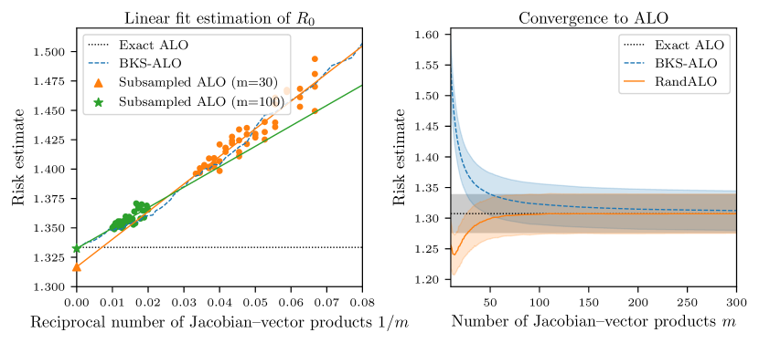
Note that is the true quantity to be estimated, and that for sufficiently large we have the approximate linear relation . Therefore, we can estimate by evaluating our plug-in estimate at several choices of and extracting the intercept term using linear regression. To avoid the need to compute additional Jacobian–vector products, we propose to take subsamples of size of the individual diagonal estimates which have already been computed, such that obtaining the averaged BKS estimate for the subsample has negligible cost. Repeating this subsampling procedure for several sufficiently large values of (e.g., ), we obtain our complete procedure, which we call RandALO, described in Algorithm 1 and demonstrated in Figure 4.
.
4 Computing Jacobian–vector products
We have thus far considered the computation of Jacobian–vector products as a black box operation available to Algorithm 1. In some cases this may be preferred, such as when the Jacobian can be computed via automatic differentiation, as recently exploited in a similar setting for computing Stein’s unbiased risk estimate (Nobel et al., 2023). However, for linear models as we focus on in this work, it is important that the Jacobian–vector products have similar computational complexity to the efficient iterative algorithms that practitioners generally use to obtain their predictive models.
We can determine the Jacobian using implicit differentiation of 1 to obtain the expression in 5 when the regularizer is twice differentiable, but in the general case of non-differentiable regularizers, subtleties arise that need to be handled carefully. We consider a simple yet powerful case, where can be written as a sum of functions with at most one point of non-differentiablity precomposed with affine transformations. Computing Jacobian–vector products then reduces to solving an equality-constrained quadratic program, as stated in the following theorem.
Theorem 2.
Let for solving 1, let be twice-differentiable and strictly convex in its second argument, and let the regularizer have the form for some , , and convex such that
-
•
is twice-differentiable everywhere,
-
•
for all , is twice-differentiable everywhere except , and
-
•
is constant in a neighborhood of .
Then for any vector , if there is a unique solution to the quadratic program
| (15) |
then .
Proof.
First we show that the uniqueness of implies that a particular matrix is invertible. Note that the optimality conditions of 15 are equivalent to
| (16) |
where is a full-rank matrix whose null space equals the intersection of the null spaces of for . For convenience, let . Rewritten more compactly, 16 is the system of linear equations
| (17) |
Seeking a contradiction, assume that there exists such that and . Then solves 17. This would imply that is not the unique solution to 15, contradicting our assumption that is unique. Therefore the matrix on the LHS is invertible (Boyd and Vandenberghe, 2004, §10.1.1).
We now turn to our main focus: applying the Implicit Function Theorem. By rewriting 1 with new constraints for , we obtain
| (18) |
For convenience, let and be the gradient of with respect to its second argument. In the neighborhood of for which is constant, this mapping from to is equal to the mapping from to given by
| (19) |
The constraints form an affine set parallel to the intersection of the null spaces of for all . Accordingly, we can write the optimality conditions of 19 as
| (20) |
where is as defined above. In order to apply the Implicit Function Theorem (Rudin, 1976, Theorem 9.28) to 20, we note that there exists an open set around , such that for all , for all . Therefore, the left-hand side is continuously differentiable on . Further, the Jacobian of the left-hand sides of 20 with respect to is given by
| (21) |
This matrix is the same as the left-hand side of 17, which we showed to be invertible above.
The conditions of this theorem are somewhat technical, but they allow us to generalize to many common regularizers of interest. The essence of the result is that when a solution is found at a non-differentiable point of a regularizer, the Jacobian has no component in the corresponding direction. We now give several examples of how to apply this theorem for a few popular regularizers.
Corollary 3.
For the elastic net penalty , the Jacobian has the form
| (24) |
where selects only the columns of from the set , when is locally constant and either or is invertible.
Proof.
Apply Theorem 2 with and for , where are the standard basis vectors, to obtain that such that satisfies
| (25) |
The constraints ensures that the columns of associated with are multiplied by , allowing the to be expressed as the minimization of the following quadratic: . This can be solved analytically to show that . Because either is invertible or , such that is invertible, is unique for any as required by the theorem. By considering for , we obtain 24. ∎
The above corollary of course recovers the standard ridge regression () and lasso () penalty Jacobians as special cases and matches the extension of ALO to the elastic net by Auddy et al. (2024). Other separable penalties such as the norm admit a similar form. However, we are not restricted to separable penalties. For example, we can also pre-transform before applying a separable penalty.
Corollary 4.
For the linearly transformed penalty , the Jacobian–vector product where is the unique optimal solution to
| (26) |
where selects only the columns of from the set when it is locally constant.
Proof.
Apply Theorem 2 with and for . ∎
The above penalty is commonly used in the compressed sensing literature, where transforms into a frame in which it should be sparse. Another non-separable example is the group lasso.
Corollary 5.
For the group lasso with disjoint idempotent subspace projection operators such that and , the Jacobian has the form
| (27) |
where for when is locally constant.
Proof.
The Hessian of a single norm component is given by
| (28) |
We can then apply Theorem 2. The linear constraint becomes for all such that , which is equivalent to restricting the system to the complementary subspace defined by . ∎
The standard group lasso where feature are partitioned into groups follows under the above corollary when are diagonal matrices with ’s indicating feature membership in each group and ’s elsewhere. We give the non-overlapping group lasso here as it has a simple closed-form Jacobian, but overlapping groups can be easily accommodated in the quadratic program formulation.
Since Theorem 2 describes the Jacobian as a quadratic program in -dimensional space, it requires a known feature representation of the data. However, we can still consider linear models in unknown feature spaces for the ridge regularizer, enabling us to apply RandALO to kernel methods.
Corollary 6.
For the ridge penalty , the Jacobian admits a formulation in terms of the kernel matrix . If and are invertible, then
| (29) |
Proof.
Without loss of generality, since is invertible, assume that . Then starting from the ridge penalty solution in Corollary 3 with and , we can introduce inside and outside the inverse to obtain
| (30) |
Bringing the on the right inside the inverse on the left as cancels terms to produce the stated expression. ∎
4.1 Alternative approaches
There are other methods to evaluate the Jacobian–vector products. By reducing a convex data fitting problem to the conic form of the optimization problem, the Jacobian–vector products can be evaluated as a system of linear equations (Agrawal et al., 2019) or via perturbations to the input solver (Paulus et al., 2024). Other work enables the minimization of non-convex least squares problems (Pineda et al., 2022). We leave extending our efficient method to particular cases of interest such as non-differentiable losses (even jointly with non-differentiable regularizers) to future work.
5 Numerical Experiments
We now demonstrate the effectiveness of RandALO on a variety of problems, including with different losses, regularizers, and models on the data. In particular, we show how RandALO is able to outperform -fold CV (typically, -fold CV as a single point of comparison) in terms of both accuracy of the risk estimate and computational cost. Unless otherwise specified, we implemented these experiments as follows.
RandALO implementation.
We wrote an open-source Python implementation of RandALO based on PyTorch (Paszke et al., 2019) available on PyPI as randalo and at https://github.com/cvxgrp/randalo, capable of accepting arbitrary black-box implementations of Jacobian–vector products.
Jacobian–vector product implementation.
We implement our Jacobian-vector products using the torch_linops library (available at https://github.com/cvxgrp/torch_linops) and SciPy (Virtanen et al., 2020) to solve the quadratic program in 15. For problems with dense data and , we compute the solution directly via the LDL factorization, for sparse data we apply the conjugate gradient (CG) method, and for large dense data we apply MINRES.
Machine learning implementation.
We used standard and well-optimized methods for fitting common models provided by scikit-learn (Pedregosa et al., 2011) for lasso, logistic regression, and cross-validation. For first-difference -regularized regression we implemented the solution using the Clarabel solver (Goulart and Chen, 2024) through CVXPY (Diamond and Boyd, 2016; Agrawal et al., 2018). For kernel logistic regression, we implement a Newton’s method solver using CG.
Hyperparameter selection.
We consider high-dimensional problems similar to those for which ALO is known to provide consistent risk estimation (Xu et al., 2021). For boxplots, we select hyperparameters roughly of the same order as the optimal parameter given the noise level such that the risks at those hyperparameters are of interest.
Risk metrics.
We consider the regression risk metric of squared error as well as the classification risk metric of misclassification error . For each risk estimate , we report the relative error from the conditional risk , with boxplots depicting 100 random trials.
Relative time.
All relative times are reported with respect to the time to fit the model according to 1 on the full training data. For CV, the time reported includes only the fitting of the models in 3, and computing after model selection would be an additional computational cost. For ALO methods, we include the original fitting of the model and add the time required to run Algorithm 1 (omitting the inflation debiasing step for BKS-ALO).
Compute environment.
We compute on Stanford’s Sherlock cluster, drawing new random data and BKS vectors each trial. We run each trial on a single core with 16GB of memory, reporting wall-clock times for each computation done.
5.1 Lasso: Efficiency and problem scaling
In this experiment, we generate and for having non-zero elements drawn as i.i.d. and . We fit a lasso model with and . We fix and set , which balances the loss and regularizer to be of the same order. The conditional squared error risk is given by
| (31) |
In Figure 1 we consider this problem for using the direct dense solver for Jacobian–vector products. Even with the highly optimized coordinate descent solver for lasso, the estimation error–computation trade-off curve for CV is entirely dominated by both BKS-ALO and RandALO. For low numbers of Jacobian–vector products , RandALO provides roughly an order of magnitude improvement in risk estimation and a small additional cost. For larger , RandALO does converge more quickly to the limiting risk estimate, but both BKS-ALO and RandALO are within the standard deviation of the conditional risk from the marginal risk, which is what CV methods provide an estimate of, and so either method could be equally trusted. We consider the same problem setup in Figure 4 where we demonstrate the debiasing improvement of RandALO over BKS-ALO.
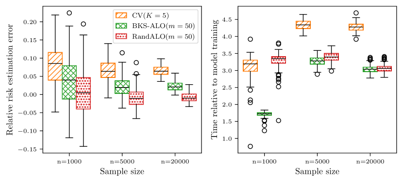
In Figure 5, we consider increasing values of . We use MINRES to compute the Jacobian–vector products for since it scales better to large . We see that the inconsistency of CV remains the same with increasing problem dimension without vanishing, while with only Jacobian–vector products, we have virtually eliminated all bias in RandALO at only a fraction of the time of -fold CV. The overhead due to applying the debiasing procedure of RandALO is substantial for , but it becomes negligible as increases.
5.2 Sparse first-difference regression
In this experiment, we demonstrate the dramatic improvement of randomized ALO over CV for non-standard problems. We now generate data in the same manner as in Section 5.1 except we let be the cumulative sum of having non-zero elements with indices selected at random without replacement and values drawn i.i.d. , such that is piecewise constant , and we let . Accordingly, we use the first-differences regularizer where
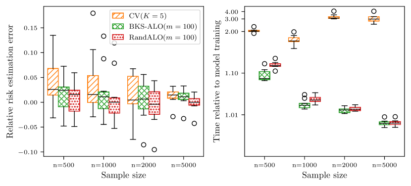
This regularizes towards being piecewise constant. We fix and . Unlike the lasso, this regularizer is used much more rarely and lacks the same highly specialized solving methods. This results in significantly slower solve times and, as shown in Figure 6, being able to avoid the expense of having to fit multiple models, instead solving the quadratic program in 26 for Jacobian–vector products, yields much improved runtime using RandALO at no cost to accuracy.
5.3 Logistic ridge regression
In this example, we demonstrate that randomized ALO works outside of squared error regression. We consider a binary classification problem using the logistic loss function used for binary classification regularized with the ridge penalty . We again consider , while for labels we let with probability for , , and having nonzero elements drawn as i.i.d. , and let otherwise. We let and and choose . We evaluate misclassification error with risk function , which has the conditional risk
| (32) |
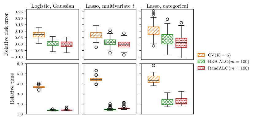
which we can compute via numerical integration with the 2-dimensional Gaussian density. We emphasize that this risk is distinct from the logistic loss used to fit the model. For this problem, we have slower solvers available than for lasso, making the overhead for randomized ALO using the direct solver for Jacobian–vector products small compared to -fold CV, as shown in Figure 7 (left).
5.4 Multivariate data
In this example we consider our first departure from known guarantees for the consistency of ALO. We consider the same setting as Section 5.1 except we let the data be drawn from a scaled multivariate -distribution. That is, where and where denotes the chi-squared distribution with degrees of freedom. We let . Since , we have the same expression for conditional risk from 31 as in the Gaussian case.
Notably, because of the instance-wise scalars , the diagonal Jacobian elements do not all concentrate to the same value, meaning that GCV, which uses where ALO uses in 5, cannot be consistent in general. However, as shown in Figure 7 (middle), ALO provides consistent risk estimation and can be implemented efficiently using our randomized method.
5.5 Categorical data
In our next example, we go even further from standard random matrix assumptions. We sample by drawing independently and uniformly from and concatenating standard basis vectors to form where . We then generate for having non-zero elements drawn as i.i.d. and . We choose and and generate as a sparse data matrix. We apply lasso with . For this problem, we have the covariance structure
| (33) |
where denotes the matrix of all ones. This gives us the conditional squared error
| (34) |
As we show in Figure 7 (right), randomized ALO is still able to provide an accurate risk estimate even for categorical data. As in the other cases, it provides a more accurate risk estimate in less time than -fold CV, here using the iterative CG solver on sparse -dimensional data.
5.6 Hyperparameter sweep
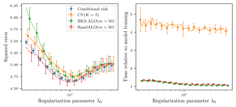
In settings where CV is particularly poorly behaved, RandALO provides a more accurate sense of how risk varies with hyperparameters. We ran an experiment using the same setup as in Section 5.1 but with , , , and . Sweeping across a whole range of lasso regularization parameters , we show in Figure 8 that RandALO provides an extremely high quality risk estimate with minimal computational overhead, eliminating nearly all of the bias of BKS-ALO and providing a significantly better risk estimate curve over CV with extremely minimal computational overhead.
| CV() | BKS-ALO() | RandALO() | ||||||||
|---|---|---|---|---|---|---|---|---|---|---|
| Conditional risk | ||||||||||
| 100 | 0 | 37 | 89 | 67 | 99 | 100 | 100 | 100 | 100 | |
| 0 | 100 | 63 | 11 | 33 | 1 | 0 | 0 | 0 | 0 | |
In fact, for this problem, the bias of CV is sufficiently severe as to yield incorrect hyperparameter selection on the basis of the risk estimate. To emphasize this, in Table 1 we show over the 100 trials how many times the choice , which is around the global minimizer, would be chosen over , which is nearly halfway to null model risk achieved around . Thus for very high-dimensional problems, the risk estimate of RandALO can produce better model selection decisions than CV, in just a fraction of the time.
5.7 Kernel logistic regression on Fashion-MNIST
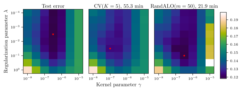
Although we have developed RandALO for linear models, this does not restrict us to models that are linear in the data space. Using Corollary 6, we can also obtain risk estimates for kernel methods with RKHS norm penalties, though with no proven guarantee that ALO provides consistent risk estimation in this setting. In this example on real data from the Fashion-MNIST dataset (Xiao et al., 2017), we apply kernel logistic regression using the same loss and regularizer as in Section 5.3 on the binary task of differentating “casual” (t-shirt, pullover, sneaker) and “formal” (shirt, coat, ankle boot) clothing. We select training samples and 20000 test samples at random and use the radial basis function kernel . The data points are -dimensional vectors of pixel intensities taking values from to .
In Figure 9, we compare the resulting risk estimates for 5-fold CV and RandALO as a function of the ridge parameter and kernel parameter . Both CV and RandALO provide biased risk estimates, and neither selects a parameter that minimizes the test error. Both do select good parameters, with CV achieving % test error and RandALO achieving % test error, compared to the best test error of %, but CV requires nearly triple the amount of computational effort to do so. RandALO provides a better risk estimate than CV where the test error is also small, but outside of the low risk basin the risk estimation is worse, such as for , which corresponds to the kernel becoming too narrow for the data and reducing the effectiveness of ALO.
6 Discussion
We have presented a randomized method for computing the approximate leave-one-out risk estimate that enables efficient hyperparameter tuning in time comparable to and often much better than -fold cross-validation. The key to our method is combining ALO with randomized diagonal estimation along with the crucial proper handling of estimation noise to reduce bias and variance, resulting in our requiring only a fairly small roughly constant number of quadratic program solves regardless of problem size, scaling very favorably to large datasets.
There are a few important extensions that we leave for subsequent work. Firstly, it is important to extend to non-differentiable losses, which include popular losses such as the hinge loss for support vector machines and the pinball loss for quantile regression. These losses are often also paired with non-differentiable regularizers such as the norm, and so it is important to be able to handle joint non-differentiability. With second derivatives of the loss arising very naturally due to the Newton step of ALO, more care is needed in obtaining the appropriate update and making the appropriate adjustments to the randomized diagonal estimation procedure to deal with special non-differentiability behavior.
Secondly, in large-scale machine learning, arguably the most common and important task is multi-class classification. Extending to this case would require first extending ALO to multidimensional outputs and then incorporating an appropriate extension of randomized “diagonal” estimation to these higher order tensors. With a proper extension to multi-class classification, RandALO could be applied to neural networks taking the Jacobian based perspective of ALO from Appendix A. Based on the results of Park et al. (2023) who showed compelling results of applying a method based on ALO for data attribution, we anticipate risk estimates based on linearized neural networks performing very well, having the potential to save precious training data from being set aside for validation.
Acknowledgements
The authors would like to thank Stephen Boyd, Alice Cortinovis, and Pratik Patil for many helpful discussions. PTN was supported in part by the National Science Foundation Graduate Research Fellowship Program under Grant No. DGE-1656518. Any opinions, findings, and conclusions or recommendations expressed in this material are those of the author(s) and do not necessarily reflect the views of the National Science Foundation. DL was supported by ARO grant 2003514594 and Stanford Data Science. EJC was supported by the Office of Naval Research grant N00014-20-1-2157, the National Science Foundation grant DMS-2032014, the Simons Foundation under award 814641. Some of the computing for this project was performed on the Sherlock cluster. The authors would like to thank Stanford University and the Stanford Research Computing Center for providing computational resources and support that contributed to these research results.
Appendix A Generic derivation of ALO
Instead of a linear model , consider an arbitrary model differentiably parameterized by . The fully trained model satisfies the first-order optimality condition
| (35) |
We seek to approximate the LOO solution , which satisfies instead
| (36) |
The key idea is to start from and follow the path of solutions that still satisfy 35; that is, they should still be the solution to a regularized empirical risk minimization problem. As we seek to satisfy 36, this leaves one degree of freedom in 35, namely, the value of , which does not appear in 36. Now following Rahnama Rad and Maleki (2020), we take a Newton step of optimization starting from towards a root of the LOO optimality condition. Under 35, this is equivalent to simply finding a root of the left out loss
| (37) |
Assuming that for any , a root must be a root of . Recall that we had only one degree of freedom in , and denote , which is a function of . Then we can apply one step of Newton’s method starting from to obtain the ALO prediction:
| (38) |
where denotes the total derivative and must be taken through both arguments of . Since derivatives of are inexpensive to evaluate, the fundamental quantity of ALO is the partial derivative , and with reparameterization into , we see that this procedure coincides exactly with 5.
Appendix B Proof of Theorem 1
The concentration result that we will leverage is the Hanson–Wright inequality for -sub-exponential random vectors, generalizing the more common result for sub-Gaussian random vectors. Here the Orlicz (quasi-)norm is defined as
| (39) |
A random variable is -sub-exponential if is finite.
Lemma 7 (Proposition 1.1 and Corollary 1.4, Götze et al., 2021).
Let be a random vector with independent components which satisfy and . Let and let be a symmetric matrix. Then for some constant depending only on , for every ,
| (40) | ||||
| (41) |
From this result we also derive the following corollary for asymmetric quadratic forms.
Corollary 8.
Let and be random vectors with independent components which satisfy and , and let be a matrix. Then for some constant depending only on , for every ,
| (42) |
Proof.
First apply Lemma 7 for
| (43) |
It is straightforward to see that and , giving us the high probability bound
| (44) |
By choosing , we obtain the stated result as an upper bound. ∎
We will also use this result on the spectral concentration for random matrices, which will allow us to conclude that certain spectral properties of the random data do not change even if a single data point is left out. Here the trace norm, or nuclear norm, is defined as .
Lemma 9 (Theorem 1, Rubio and Mestre, 2011).
Let be a random matrix consisting of i.i.d. random variables that have mean 0, variance 1, and finite absolute moment of order for some . Let and be positive semidefinite matrices with operator norm uniformly bounded in , and let . Then, for , as such that , we have for any having trace norm uniformly bounded in ,
| (45) |
where does not depend on but solves and .
Proof of Theorem 1.
Without loss of generality, since can be absorbed into for an equivalent problem with and , assume and is uniformly bounded. Furthermore, it suffices to prove the result for . Let denote the th row of , having the form , and let denote with removed, such that is independent of . Similarly, let denote with removed.
First, since and are independent and zero mean, . It remains then to characterize the variance. By the Woodbury identity, it is straightforward to obtain that
| (46) |
The first term, , is simply . To determine the value of , we can first apply Lemma 7 with and . Note that both and can be uniformly upper bounded by for some constant . Therefore,
| (47) |
For every , if we sum the right-hand side over to , the sum of probabilities is finite. Thus by the Borel–Cantelli lemma, we have . Now applying Lemma 9 with , we see that the trace term takes asymptotically almost surely the same value regardless of whether is left out of or not, since . Thus for .
Next, we need to apply a central limit theorem to obtain Gaussianity of the error. Note that
| (48) |
Since are independent of the remaining quantities, we can apply Lyapunov’s central limit theorem provided we can show that the other terms are not too sparse. That is, we need to show that for some ,
| (49) |
To deal with the numerator, note that by the Woodbury identity,
| (50) |
where is the matrix with both the th and th rows removed. We can then apply Corollary 8 with , , and , which must have and upper bounded by . Choosing , we have
| (51) |
Using a union bound over , we can therefore say that all of these terms are bounded by with probability at least . With similar probability, the denominator of 50 also concentrates for all . Thus, we have
| (52) |
where “” indicates that the inequality holds with sufficiently high probability that the sum of the complementary events across are finite, such that we can apply the Borel–Cantelli lemma to obtain almost sure convergence. We now need only show that the denominator of 49 is lower bounded. Making similar concentration arguments as above using Lemma 7, it is sufficient to show that
| (53) |
is uniformly bounded away from 0. Since has all eigenvalues bounded away from zero, we can ignore it, and so we need only lower bound the smallest singular value of . Again since and have lower bounded eigenvalues, we need only the smallest singular value of to be lower bounded by , which we have by classical results in random matrix theory (Bai and Silverstein, 1998) almost surely. Then , and so we can apply Lyapunov’s central limit theorem to obtain that almost surely over ,
| (54) |
To get a simpler value for the expression in 53, recall that the derivative of a matrix resolvent is a second order resolvent: , meaning that we can apply Lemma 9 to second-order resolvent polynomials as well (such “asymptotic equivalences” hold for derivatives provided all sequences are bounded as they are in our case; see, Theorem 11 of Dobriban and Sheng, 2020), allowing us to replace with :
| (55) |
It remains to show that the element-wise noise of is asymptotically conditionally uncorrelated. That is, we need to show that for .
| (56) |
Note that this term can be expressed as a sum , and that we can therefore exploit the fact that . Observe that we can never have or , and of course . The remaining term, where and , vanishes:
| (57) |
which follows by a similar arguments based on Corollary 8 made earlier in the proof (first apply the Woodbury identity twice to extract and from the inverse as a shrinking scalar, then apply 51), proving the stated result for . To account for , we can simply average Gaussian variables. ∎
References
- Agrawal et al. (2018) A. Agrawal, R. Verschueren, S. Diamond, and S. Boyd. A rewriting system for convex optimization problems. Journal of Control and Decision, 5(1):42–60, 2018.
- Agrawal et al. (2019) A. Agrawal, S. Barratt, S. Boyd, E. Busseti, and W. Moursi. Differentiating through a cone program. Journal of Applied and Numerical Optimization, 1(2):107–115, 2019. doi:10.23952/jano.1.2019.2.02.
- Arlot and Celisse (2010) S. Arlot and A. Celisse. A survey of cross-validation procedures for model selection. Statistics Surveys, 4:40–79, 2010. doi:10.1214/09-SS054.
- Auddy et al. (2024) A. Auddy, H. Zou, K. Rahnama Rad, and A. Maleki. Approximate leave-one-out cross validation for regression with regularizers. In Proceedngs of the 27th International Conference on Artificial Intelligence and Statistics, pages 2377–2385, 2024.
- Bai and Silverstein (1998) Z. D. Bai and J. W. Silverstein. No eigenvalues outside the support of the limiting spectral distribution of large-dimensional sample covariance matrices. The Annals of Probability, 26(1):316–345, 1998. doi:10.1214/aop/1022855421.
- Baston and Nakatsukasa (2022) R. A. Baston and Y. Nakatsukasa. Stochastic diagonal estimation: probabilistic bounds and an improved algorithm. arXiv:2201.10684, 2022.
- Bates et al. (2024) S. Bates, T. Hastie, and R. Tibshirani. Cross-validation: What does it estimate and how well does it do it? Journal of the American Statistical Association, 119(546):1434–1445, 2024. doi:10.1080/01621459.2023.2197686.
- Bekas et al. (2007) C. Bekas, E. Kokiopoulou, and Y. Saad. An estimator for the diagonal of a matrix. Applied Numerical Mathematics, 57(11):1214–1229, 2007. doi:10.1016/j.apnum.2007.01.003.
- Bellec (2023) P. C. Bellec. Out-of-sample error estimation for M-estimators with convex penalty. Information and Inference: A Journal of the IMA, 12(4):2782–2817, 2023. doi:10.1093/imaiai/iaad031.
- Boyd and Vandenberghe (2004) S. Boyd and L. Vandenberghe. Convex Optimization. Cambridge University Press, 2004. ISBN 0521833787.
- Cawley and Talbot (2008) G. C. Cawley and N. L. C. Talbot. Efficient approximate leave-one-out cross-validation for kernel logistic regression. Machine Learning, 71(2):243–264, 2008. doi:10.1007/s10994-008-5055-9.
- Craven and Wahba (1978) P. Craven and G. Wahba. Smoothing noisy data with spline functions. Numerische Mathematik, 31(4):377–403, 1978. doi:10.1007/BF01404567.
- Diamond and Boyd (2016) S. Diamond and S. Boyd. CVXPY: A Python-embedded modeling language for convex optimization. Journal of Machine Learning Research, 17(83):1–5, 2016.
- Dobriban and Sheng (2020) E. Dobriban and Y. Sheng. WONDER: Weighted one-shot distributed ridge regression in high dimensions. Journal of Machine Learning Research, 21(66):1–52, 2020.
- Donoho et al. (2011) D. L. Donoho, A. Maleki, and A. Montanari. The noise-sensitivity phase transition in compressed sensing. IEEE Transactions on Information Theory, 57(10):6920–6941, 2011. doi:10.1109/TIT.2011.2165823.
- Epperly et al. (2024) E. N. Epperly, J. A. Tropp, and R. J. Webber. XTrace: Making the most of every sample in stochastic trace estimation. SIAM Journal on Matrix Analysis and Applications, 45(1):1–23, 2024. doi:10.1137/23M1548323.
- Golub and Van Loan (2013) G. H. Golub and C. F. Van Loan. Matrix Computations. John Hopkins University Press, 4 edition, 2013.
- Götze et al. (2021) F. Götze, H. Sambale, and A. Sinulis. Concentration inequalities for polynomials in -sub-exponential random variables. Electronic Journal of Probability, 26:1–22, 2021. doi:10.1214/21-EJP606.
- Goulart and Chen (2024) P. J. Goulart and Y. Chen. Clarabel: An interior-point solver for conic programs with quadratic objectives. arXiv:2405.12762, 2024.
- Hastie et al. (2009) T. Hastie, R. Tibshirani, and J. Friedman. The Elements of Statistical Learning. Springer Series in Statistics, 2nd edition, 2009. doi:10.1007/978-0-387-84858-7.
- Hutchinson (1990) M. Hutchinson. A stochastic estimator of the trace of the influence matrix for Laplacian smoothing splines. Communications in Statistics – Simulation and Computation, 19(2):433–450, 1990. doi:10.1080/03610919008812866.
- Luo et al. (2023) Y. Luo, Z. Ren, and R. Barber. Iterative approximate cross-validation. In Proceedings of the 40th International Conference on Machine Learning, pages 23083–23102, 2023.
- Meyer et al. (2021) R. A. Meyer, C. Musco, C. Musco, and D. P. Woodruff. Hutch++: Optimal stochastic trace estimation. In The 2021 Symposium on Simplicity in Algorithms (SOSA), pages 142–155, 2021. doi:10.1137/1.9781611976496.16.
- Nobel et al. (2023) P. Nobel, E. Candès, and S. Boyd. Tractable evaluation of stein’s unbiased risk estimate with convex regularizers. IEEE Transactions on Signal Processing, 71:4330–4341, 2023. doi:10.1109/TSP.2023.3323046.
- Park et al. (2023) S. M. Park, K. Georgiev, A. Ilyas, G. Leclerc, and A. Ma̧dry. TRAK: Attributing model behavior at scale. In Proceedings of the 40th International Conference on Machine Learning, pages 27074–27113, 2023.
- Paszke et al. (2019) A. Paszke, S. Gross, F. Massa, A. Lerer, J. Bradbury, G. Chanan, T. Killeen, Z. Lin, N. Gimelshein, L. Antiga, A. Desmaison, A. Kopf, E. Yang, Z. DeVito, M. Raison, A. Tejani, S. Chilamkurthy, B. Steiner, L. Fang, J. Bai, and S. Chintala. PyTorch: An imperative style, high-performance deep learning library. In Advances in Neural Information Processing Systems, volume 32, 2019.
- Patil and LeJeune (2024) P. Patil and D. LeJeune. Asymptotically free sketched ridge ensembles: Risks, cross-validation, and tuning. In Proceedings of the 12th International Conference on Learning Representations, 2024.
- Patil et al. (2021) P. Patil, Y. Wei, A. Rinaldo, and R. Tibshirani. Uniform consistency of cross-validation estimators for high-dimensional ridge regression. In Proceedings of the 24th International Conference on Artificial Intelligence and Statistics, 2021.
- Paulus et al. (2024) A. Paulus, G. Martius, and V. Musil. LPGD: A general framework for backpropagation through embedded optimization layers. arXiv:2407.05920, 2024.
- Pedregosa et al. (2011) F. Pedregosa, G. Varoquaux, A. Gramfort, V. Michel, B. Thirion, O. Grisel, M. Blondel, P. Prettenhofer, R. Weiss, V. Dubourg, J. Vanderplas, A. Passos, D. Cournapeau, M. Brucher, M. Perrot, and E. Duchesnay. Scikit-learn: Machine learning in Python. Journal of Machine Learning Research, 12:2825–2830, 2011.
- Pineda et al. (2022) L. Pineda, T. Fan, M. Monge, S. Venkataraman, P. Sodhi, R. T. Q. Chen, J. Ortiz, D. DeTone, A. Wang, S. Anderson, J. Dong, B. Amos, and M. Mukadam. Theseus: A library for differentiable nonlinear optimization. In Advances in Neural Information Processing Systems, volume 35, pages 3801–3818, 2022.
- Pregibon (1981) D. Pregibon. Logistic regression diagnostics. The Annals of Statistics, 9(4):705–724, 1981. doi:10.1214/aos/1176345513.
- Rahnama Rad and Maleki (2020) K. Rahnama Rad and A. Maleki. A scalable estimate of the out-of-sample prediction error via approximate leave-one-out cross-validation. Journal of the Royal Statistical Society Series B: Statistical Methodology, 82(4):965–996, 2020. doi:10.1111/rssb.12374.
- Rubio and Mestre (2011) F. Rubio and X. Mestre. Spectral convergence for a general class of random matrices. Statistics & Probability Letters, 81(5):592–602, 2011. doi:10.1016/j.spl.2011.01.004.
- Rudin (1976) W. Rudin. Principles of Mathematical Analysis, Third Edition. McGraw-Hill Science Engineering Math, 3rd edition, 1976.
- Stephenson and Broderick (2020) W. Stephenson and T. Broderick. Approximate cross-validation in high dimensions with guarantees. In Proceedings of the 23rd International Conference on Artificial Intelligence and Statistics, pages 2424–2434, 2020.
- Virtanen et al. (2020) P. Virtanen, R. Gommers, T. E. Oliphant, M. Haberland, T. Reddy, D. Cournapeau, E. Burovski, P. Peterson, W. Weckesser, J. Bright, S. J. van der Walt, M. Brett, J. Wilson, K. J. Millman, N. Mayorov, A. R. J. Nelson, E. Jones, R. Kern, E. Larson, C. J. Carey, İ. Polat, Y. Feng, E. W. Moore, J. VanderPlas, D. Laxalde, J. Perktold, R. Cimrman, I. Henriksen, E. A. Quintero, C. R. Harris, A. M. Archibald, A. H. Ribeiro, F. Pedregosa, P. van Mulbregt, and SciPy 1.0 Contributors. SciPy 1.0: Fundamental algorithms for scientific computing in python. Nature Methods, 17:261–272, 2020. doi:10.1038/s41592-019-0686-2.
- Xiao et al. (2017) H. Xiao, K. Rasul, and R. Vollgraf. Fashion-MNIST: a novel image dataset for benchmarking machine learning algorithms. arXiv:1708.07747, 2017.
- Xu et al. (2021) J. Xu, A. Maleki, K. Rahnama Rad, and D. Hsu. Consistent risk estimation in moderately high-dimensional linear regression. IEEE Transactions on Information Theory, 67(9):5997–6030, 2021. doi:10.1109/TIT.2021.3095375.
- Zhang and Yang (2015) Y. Zhang and Y. Yang. Cross-validation for selecting a model selection procedure. Journal of Econometrics, 187(1):95–112, 2015. doi:10.1016/j.jeconom.2015.02.006.