Generalizing Alignment Paradigm of
Text-to-Image Generation with Preferences
through $f$-divergence Minimization

Abstract

Direct Preference Optimization (DPO) has recently expanded its successful application from aligning large language models (LLMs) to aligning text-to-image models with human preferences, which has generated considerable interest within the community. However, we have observed that these approaches rely solely on minimizing the reverse Kullback-Leibler divergence during alignment process between the fine-tuned model and the reference model, neglecting the incorporation of other divergence constraints. In this study, we focus on extending reverse Kullback-Leibler divergence in the alignment paradigm of text-to-image models to $f$-divergence, which aims to garner better alignment performance as well as good generation diversity. We provide the generalized formula of the alignment paradigm under the $f$-divergence condition and thoroughly analyze the impact of different divergence constraints on alignment process from the perspective of gradient fields. We conduct comprehensive evaluation on image-text alignment performance, human value alignment performance and generation diversity performance under different divergence constraints, and the results indicate that alignment based on Jensen-Shannon divergence achieves the best trade-off among them. The option of divergence employed for aligning text-to-image models significantly impacts the trade-off between alignment performance (especially human value alignment) and generation diversity, which highlights the necessity of selecting an appropriate divergence for practical applications.

1 Introduction

Text-to-image generative models have witnessed significant advancements in recent years [1, 2, 3, 4]. When presented with appropriate textual prompts, they are capable of generating high-fidelity images that are semantically coherent with the provided descriptions, which spans a diverse range of topics, piquing significant public interest in their potential applications and societal implications. Existing self-supervised pre-trained generators, although advanced, still exhibit imperfections, with a significant challenge being their alignment with human preferences [5].

Reinforcement Learning from Human Feedback (RLHF) has established itself as a pivotal research endeavor, demonstrating notable efficacy in aligning text-to-image models with human preferences [6, 7, 8]. Faced with the intricate challenge of defining an objective that authentically encapsulates human preferences in the realm of Reinforcement Learning from Human Feedback (RLHF), researchers conventionally assemble a dataset to mirror such preferences through comparative assessments of model-generated outputs [6, 9]. Then, a reward model is trained based on Bradley-Terry model [10], inferring human preferences from the collected dataset. And the text-to-image model is fine-tuned with a reinforcement learning (RL) pipeline. It is noteworthy that such process is conducted while ensuring the model remains closely with its original form, which is achieved by employing a reverse Kullback-Leibler divergence penalty. Significant complexity has been introduced to the RLHF pipeline due to the requirement to train a separate reward model, even though it is somewhat effective. Moreover, Reinforcement learning pipelines also present notable challenges in terms of stability and memory demands towards alignment process of text-to-image models.

Recent research has demonstrated significant success in fine-tuning large language models (LLMs) using methods based on implicit rewards, specially the Direct Preference Optimization (DPO) [11]. Application of similar fine-tuning techniques to text-to-image models has also produced promising results, such as Diffusion-DPO [12], D3PO [13]. Such results have raisen significant interest within the community regarding the alignment of text-to-image models with human value through the methodology of utilizing implicit rewards. Furthermore, researchers have devoted significant efforts to applying such paradigm of aligning human value to text-to-image models, including SPO [14], NCPPO [15], DNO[16], and so on. However, it is the situation that existing research of text-to-image generation alignment predominantly targets solutions subject to the constraint of the reverse Kullback-Leibler divergence, with notable underexploitation of strategies that integrate other types of divergences.

It has been pointed out that models would overfit due to repeated fine-tuning on a few images, thus leading to reduced output diversity [17]. In the alignment of large language models, similar challenges exist; and some studies [18, 19] have highlighted that the mode-seeking property of reverse KL divergence tends to reduce diversity in generated outputs, which can constrain the model’s potential. Studies on aligning large language models [20, 21] indicate that the problem of diversity reduction caused by fine-tuning can be alleviated by incorporating diverse divergence constraints. Therefore, in this study, we also explore the effects of employing diverse divergence constraints on the generation diversity.

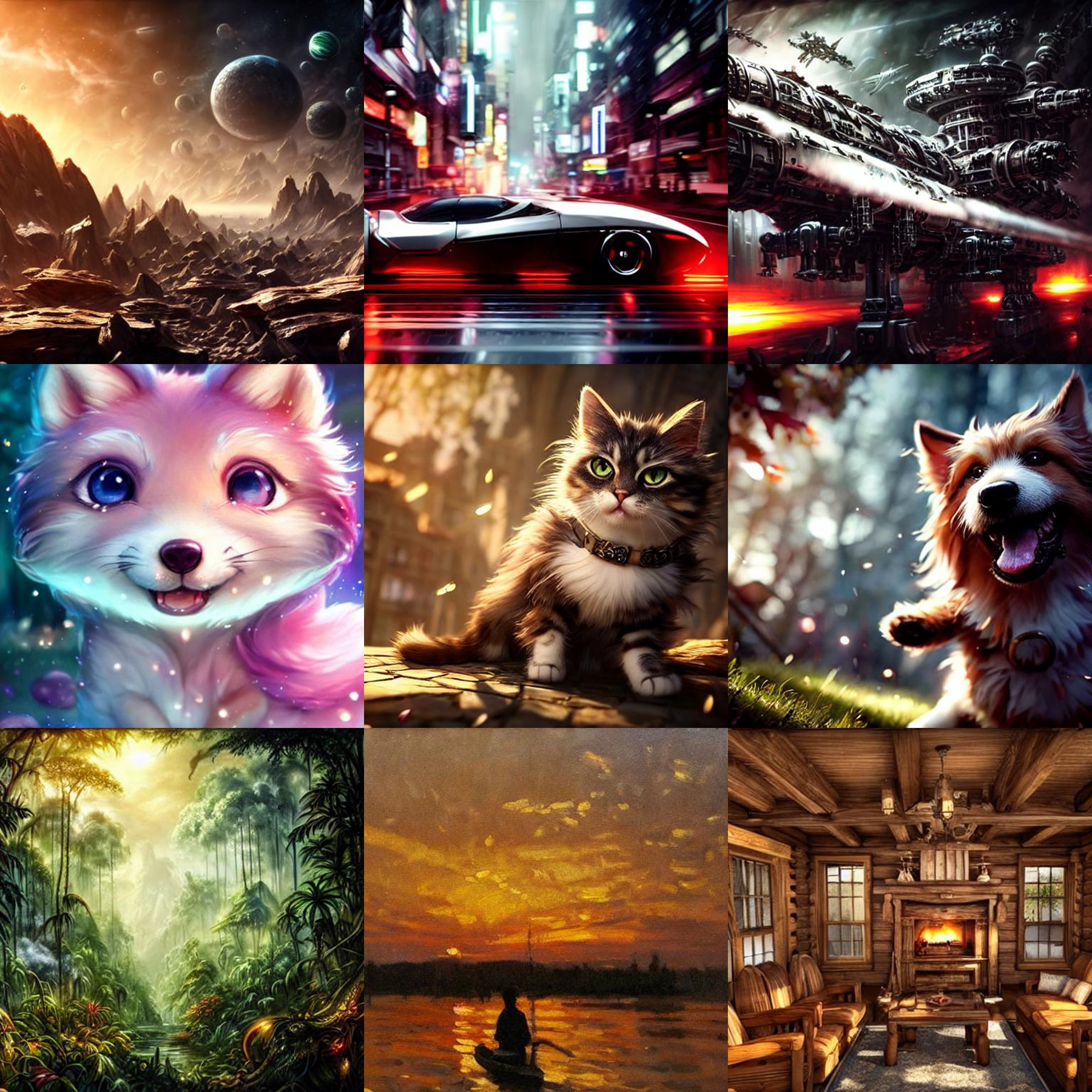
Figure 1: Examples of image generated by the model aligned using the Jensen-Shannon divergence constraint.

In this study, we generalize the alignment of text-to-image models based on reverse Kullback-Leibler divergence to a framework based on $\mathit{f}$-divergence constraints, which encompasses a wider range of divergences, including Jensen-Shannon divergence, forward Kullback-Leibler divergence, $\alpha$-divergence, and so on. We comprehensively analyze the impact of diverse divergence constraints on the alignment process from the perspective of gradient fields. Furthermore, we set Step-aware Preference Optimization (SPO) [14] as our benchmark method, utilize Stable Diffusion V1.5 [22] as our benchmark model, and assess on the test split of HPS-V2 [9] with different divergence constraints. Evaluations are carried out to examine the performance of image-text alignment, human value alignment, and generation diversity, which also aim to discern the certain divergence most effectively balances these three aspects. Our results indicate that Jensen-Shannon divergence successfully strikes the ideal equilibrium among the three criteria examined, while also achieving the highest standard in human value alignment performance. Therefore, in text-to-image alignment, judicious selection of the divergence constraint, tailored to the specific alignment requirements, is paramount. In Figure 1, we present several images generated by the model that have been aligned under the Jensen-Shannon divergence.

To the best of our knowledge, this is the first work to apply different divergence constraints to text-to-image alignment paradigm. Our contributions are summarized as follows: (1) Generalized alignment formula: we propose a generalized formula for text-to-image generation alignment, aiming to provide more choices on divergence constraints in alignment execution. (2) Thorough alignment process analysis: we comprehensively analyze the impact of different divergence constraints on alignment process from the perspective of gradient fields. (3) Extensive alignment evaluations: we conducted extensive evaluations on text-to-image generation alignment, meticulously assessing both alignment performance (image-text alignment and human value alignment) and generation diversity.

2 Related Work

2.1 Aligning Text-to-Image Model with Preferences

Recently, inspired by the alignment approaches based on human preferences, notably exemplified by methods such as direct preference optimization (DPO) [11], eliminating the need for explicit reward models and showing their significant success on Large Language Models (LLMs), and then garnering substantial attention within the community on the development of offline alignment for text-to-image diffusion models. Diffusion-DPO [12] enables text-to-image diffusion models to directly learn from human feedback in an open-vocabulary setting, and fine-tunes them on the contains Pick-a-Pic [6] dataset with image preference pairs. Direct Preference for Denoising Diffusion Policy Optimization (D3PO) [13] proposes a method on generating pairs of images from the same prompt and identifying the preferred and dispreferred images with the help of human evaluators. Step-aware Preference Optimization (SPO) [14] propose an approach that preferences at each step should be assessed and it utilizes a step-aware preference model and a step-wise resampler to ensure accurate step-aware preference alignment. DenseReward method [23] proposes enhancing the DPO scheme by incorporating a temporal discounting approach, which prioritizes the initial denoising steps. Noise-Conditioned Perceptual Preference Optimization (NCPPO) [15] proposes that the optimization process should aligns with human perceptual features, instead of the less informative pixel space. Direct Noise Optimization (DNO) [16] optimizes noise during the sampling process of text-to-image diffusion models. PopAlign [24] is an approach for population-level preference optimization, mitigating the biases of pretrained text-to-image diffusion models. Diffusion-KTO [25] generalizes the human utility maximization framework to the alignment of text-to-image diffusion models. While these studies have demonstrated impressive results in addressing the text-to-image alignment challenge, we also notice that they all rely on reverse Kullback-Leibler divergence to minimize the discrepancy between the fine-tuned model and the reference model.

2.2 $f$-divergence utilized in Generation Models

In previous studies, researchers have extensively examined the application of $f$-divergences in generative models. In the classical work done by [26], the concept of Generative Adversarial Networks (GANs) and their relationship to the Jensen-Shannon divergence are introduced. $f$-GAN [27] proposes that the variational expression of the $f$-divergence can be regarded as the loss function for Generative Adversarial Networks (GANs). Wasserstein-GAN [28] offers theoretical insights into the connection between the choice of divergences and the convergence of probability distributions. Moreover, in the work [29], it is proposed that utilizing various divergences and metrics can result in divergent trade-offs, and distinct evaluations tend to favor specific models. The application of $f$-divergence has also been observed in large language model alignment tasks. $f$-DPG [20] shows that Jensen-Shannon divergence strikes a good balance between different competing objectives, and often significantly outperforming the reverse Kullback-Leibler divergence. $f$-DPO [21] generalizes the framework of DPO by incorporating diverse divergence constraints; and it shows that by adjusting the divergence regularization, we can achieve a better balance between the alignment performance and the generation diversity.

3 Preliminary

3.1 $f$-divergence

For any convex function $f(x):\mathbb{R}^{+}\rightarrow\mathbb{R}$ with $f(1)=0$, and $p_{1},p_{2}$ are two distributions over a discrete set $\mathcal{X}$, the $f$-divergence between $p_{1}$ and $p_{2}$ can be defined as [30]:

$$D_{f}(p_{1}||p_{2})=\mathbb{E}_{x\sim p_{2}}\left[f\left(\frac{p_{1}(x)}{p_{2}(x)}\right)+f^{\prime}(\infty)p_{1}(p_{2}=0)\right],$$

where $f^{\prime}(\infty)=\lim\limits_{t\rightarrow 0}tf(\frac{1}{t})$ [31], $p_{1}(p_{2}=0)=0$ is the $p_{1}$-mass of the set {$x\in\mathcal{X}:p_{2}(x)=0$}. Under normal circumstances, we can make the assumption that the support set of $p_{1}$ is dominated by the support set of $p_{2}$, i.e. $Supp(p_{1})\subset Supp(p_{2})$, and then we can have $p_{1}(p_{2}=0)=0$. Hence, the aforementioned definition can be simplified as:

$$D_{f}(p_{1}||p_{2})=\mathbb{E}_{x\sim p_{2}}\left[f\left(\frac{p_{1}(x)}{p_{2}(x)}\right)\right]$$

For different functions $f(x)$, the $f$-divergence class encompasses a wide range of commonly employed divergence measures, such as reverse Kullback-Leibler (KL) divergence, forward Kullback-Leibler (KL) divergence, $\alpha$-divergence ($\alpha\in(0,1)$), Jensen-Shannon (JS) divergence, and so on.

$f-$divergence	$f(x)$	$f^{\prime}(x)$	$f^{\prime\prime}(x)$
Reverse KL	$x\log x$	$\log x+1$	$\frac{1}{x}$
Forward KL	$-\log x$	$-\frac{1}{x}$	$\frac{1}{x^{2}}$
$\alpha$-divergence	$\frac{x^{1-\alpha}-(1-\alpha)x-\alpha}{\alpha(\alpha-1)}$	$\frac{1-x^{-\alpha}}{\alpha}$	$\frac{1}{x^{\alpha+1}}$
JS divergence	$x\log\frac{2x}{x+1}+\log\frac{2}{x+1}$	$\log\frac{2x}{1+x}$	$\frac{1}{x(1+x)}$

Table 1: Several commonly used $f$-divergence with their derivatives and second derivatives.

In previous studies, reverse KL divergence can be regarded as a specific instance of $\alpha$-divergence with $\alpha=0$; and forward KL divergence as a specific instance of $\alpha$-divergence with $\alpha=1$. We summarize several commonly used $f$-divergence, the derivatives and the second derivatives in Table 1.

4 Method

Much like in the alignment tasks of large language models, there are many concepts that are analogous in the alignment tasks of text-to-image models, and we start by elucidating these parallels. Firstly, the question input of LLMs is akin to the text (condition) input of T2I models, i.e. $x\rightarrow c$; and the output answer of LLMs is akin to the generated image of T2I models, i.e. $y\rightarrow x_{0}$. Moreover, the policy of LLMs parallels the sampling probability of T2I models (especially diffusion models), i.e. $\pi(y|x)\rightarrow p(x_{0:T}|c)$. Finally, the preference data for output answers of LLMs is analogous to the preference data for generated images of T2I models, i.e. $(x,y_{w},y_{l})\rightarrow(c,x_{0}^{w},x_{0}^{l})$. In the following subsections, we first derive the generalized formula of alignment objective function. Then, we analyze the gradient field of different divergences on the alignment process with respect to the objective function and comprehensively analyze the impact of diverse divergence constraints on alignment performance.

4.1 Generalized Formula

In previous studies of Reinforcement Learning from Human Feedback (RLHF), researchers typically aim to maximize the reward function ($r(c,x_{0:T})$) while penalizing the reverse KL divergence between the fine-tuned model and the original model to prevent it from collapsing during training. In our study, we generalize such penalty constraint from the reverse KL divergence ($D_{\text{KL}}\left(p_{\theta}(x_{0:T}|c),p_{\text{ref}}(x_{0:T}|c)\right)$) to the $f$-divergence ($D_{f}\left(p_{\theta}(x_{0:T}|c),p_{\text{ref}}(x_{0:T}|c)\right)$).

We reframe the reinforcement learning objective function as an optimal problem, presenting its formulation as follows:

$$\begin{split}\arg\max\limits_{p_{\theta}}\mathbb{E}_{c\sim p_{c},x_{0:T}\sim p_{\theta}(x_{0:T}|c)}\big{[}r(c,x_{0:T})\big{]}&-\beta D_{f}\Big{(}p_{\theta}(x_{0:T}|c),p_{\text{ref}}(x_{0:T}|c)\Big{)}\\ \text{s.t.}\quad\sum\limits_{x_{0:T}}p_{\theta}(x_{0:T}|c)=1&;\forall x_{0:T}\quad p_{\theta}(x_{0:T}|c)\geq 0\end{split}$$

Such optimization problem can be addressed through the Karush-Kuhn-Tucker (KKT) conditions. Firstly, according to the definition of $f$-divergence, we construct the following Lagrangian function:

$$\begin{split}\mathcal{L}(p_{\theta}(x_{0:T}|c),\lambda,\zeta(x_{0:T}))=\mathbb{E}_{c\sim p_{c},x_{0:T}\sim p_{\theta}}\big{[}&r(c,x_{0:T})\big{]}-\beta\mathbb{E}_{p_{\text{ref}}}f\Bigg{(}\frac{p_{\theta}(x_{0:T}|c)}{p_{\text{ref}}(x_{0:T}|c)}\Bigg{)}\\ &-\lambda\left(\sum\limits_{x_{0:T}}p_{\theta}(x_{0:T})-1\right)+\sum\limits_{x_{0:T}}\zeta(x_{0:T})p_{\theta}(x_{0:T}|c)\end{split}$$

Furthermore, we can derive the Theorem 1 from the Stationarity Condition and Complementary Slackness of the Karush-Kuhn-Tucker (KKT) conditions, i.e.

$$\left\{\begin{aligned} &\nabla_{p_{\theta}(x_{0:T}|c)}\mathcal{L}(p_{\theta}(x_{0:T}|c),\lambda,\zeta(x_{0:T}))=0;\\ &\forall x_{0:T},\zeta(x_{0:T})p_{\theta}(x_{0:T}|c)=0.\end{aligned}\right.$$

Theorem 1.

If $p_{\mathrm{ref}}(x_{0:T}|c)>0$ holds for all condition $c$, $f^{\prime}(x)$ is an invertible function and $0$ is not in the definition domain of function $f^{\prime}(x)$, the reward class consistent with Bradley-Terrry model can be reparameterized with the sampling probability $p_{\theta}(x_{0:T}|c)$ and the reference sampling probability $p_{\mathrm{ref}}(x_{0:T}|c)$ as:

$$r(c,x_{0:T})=\beta f^{\prime}\Bigg{(}\frac{p_{\theta}(x_{0:T}|c)}{p_{\text{ref}}(x_{0:T}|c)}\Bigg{)}+\mathrm{const}$$ (1)

As shown in Theorem 1, the reward function can be represented by a sampling probability $p_{\theta}(x_{0:T}|c)$, a reference sampling probability $p_{\text{ref}}(x_{0:T}|c)$, and a constant $\lambda$ that is independent of $x_{0:T}$. Finally, substituting Equation (1) into the Bradley-Terrry model [10] enables us to derive the generalized formula of text-to-image generation with preferences in Theorem 2.

Theorem 2.

In the substitution process of Bradley-Terry model, the constant $\lambda$ is independent of $x_{0:T}$ and thus can be canceled out, resulting in the following form:

$$\mathcal{L}(\theta)=\mathbb{E}_{\begin{subarray}{c}(c,x_{0}^{w},x_{0}^{l})\sim\mathcal{D},\\ x_{1:T}^{w}\sim p_{\theta}(x_{1:T}^{w}|x_{0}^{w},c),\\ x_{1:T}^{l}\sim p_{\theta}(x_{1:T}^{l}|x_{0}^{l},c).\end{subarray}}-\log\sigma\left[\beta f^{\prime}\left(\frac{p_{\theta}(x_{0:T}^{w}|c)}{p_{\text{ref}}(x_{0:T}^{w}|c)}\right)-\beta f^{\prime}\left(\frac{p_{\theta}(x_{0:T}^{l}|c)}{p_{\text{ref}}(x_{0:T}^{l}|c)}\right)\right]$$ (2)

where $\sigma(\cdot)$ is the Sigmoid function; $f^{\prime}(\cdot)$ represents the derivatives of $f(\cdot)$, as listed in Table 1; $\beta$ is the penalty coefficient.

So far, we have derived the generalized formula for text-to-image generation alignment with preferences. With different divergence constraint choices, we can obtain diverse alignment objectives, thereby offering more options for the alignment process.

4.2 Analysis on Gradient Fields of Alignment Process

In this section, we delve into the gradient fields of alignment objective functions derived from various $f$-divergence, which aims to further elucidate the intricate mechanisms underlying the alignment process.

Let’s abstract from the specific details of $f^{\prime}(\cdot)$, and concentrate instead on a more general formulation of the loss function:

$$\mathcal{L}_{f}\left(\mathrm{X}_{1},\mathrm{X}_{2}\right)=-\mathbb{E}\Big{[}\log\sigma\big{(}\beta f^{\prime}(\mathrm{X}_{1})-\beta f^{\prime}(\mathrm{X}_{2})\big{)}\Big{]}$$ (3)

where $\mathrm{X_{1}}$ is the training win ratio, and is equivalent to $\frac{p_{\theta}(x_{0:T}^{w}|c)}{p_{\text{ref}}(x_{0:T}^{w}|c)}$ ; similarly, $\mathrm{X}_{2}$ is the training loss ratio, and is identical to $\frac{p_{\theta}(x_{0:T}^{l}|c)}{p_{\text{ref}}(x_{0:T}^{l}|c)}$. We present the gradients of Equation (3) with respect to $\mathrm{X_{1}}$ and $\mathrm{X_{2}}$ in the ensuing Theorem 3:

Theorem 3.

The partial derivatives (gradients) of $\mathrm{X_{1}}$ and $\mathrm{X_{2}}$ resulting from Equation (3) can be expressed as follows:

$$\left\{\begin{aligned} \frac{\partial\mathcal{L}_{f}(\mathrm{X_{1}},\mathrm{X_{2}})}{\partial\mathrm{X_{1}}}=-\beta\left(1-\sigma\left(\beta f^{\prime}(\mathrm{X}_{1})-\beta f^{\prime}(\mathrm{X}_{2})\right)\right)f^{\prime\prime}(\mathrm{X}_{1})\\ \frac{\partial\mathcal{L}_{f}(\mathrm{X_{1}},\mathrm{X_{2}})}{\partial\mathrm{X_{2}}}=\beta\left(1-\sigma\left(\beta f^{\prime}(\mathrm{X}_{1})-\beta f^{\prime}(\mathrm{X}_{2})\right)\right)f^{\prime\prime}(\mathrm{X}_{2})\end{aligned}\right.$$

Thus, the gradient ratio of $\mathcal{L}_{f}(\mathrm{X_{1}},\mathrm{X_{2}})$ between enhancement in probability for human-preferred responses ($\mathrm{X}_{1}$) and reduction in probability for human-dispreferred responses ($\mathrm{X}_{2}$) has the expression:

$$\Bigg{|}\frac{\partial\mathcal{L}_{f}(\mathrm{X_{1}},\mathrm{X_{2}})}{\partial\mathrm{X_{1}}}/\frac{\partial\mathcal{L}_{f}(\mathrm{X_{1}},\mathrm{X_{2}})}{\partial\mathrm{X_{2}}}\Bigg{|}=\frac{f^{\prime\prime}(\mathrm{X}_{1})}{f^{\prime\prime}(\mathrm{X}_{2})}$$ (4)

Referencing Table 1, different divergences yield distinct gradient ratios. If selected divergence is reverse Kullback-Leibler divergence, the gradient ratio is $\frac{\mathrm{X}_{2}}{\mathrm{X}_{1}}$; if selected divergence is Jensen-Shannon divergence, the gradient ratio is $\frac{\mathrm{X}_{2}\cdot(\mathrm{X}_{2}+1)}{\mathrm{X}_{1}\cdot(\mathrm{X}_{1}+1)}$; if selected divergence is $\alpha$-divergence, the gradient ratio is $\frac{\mathrm{X}_{2}^{1+\alpha}}{\mathrm{X}_{1}^{1+\alpha}}$; if selected divergence is forward Kullback-Leibler divergence, the gradient ratio is $\frac{\mathrm{X}_{2}^{2}}{\mathrm{X}_{1}^{2}}$. Previous studies [32, 33] present the results of original DPO framework, focusing particularly on its application in the context of reverse Kullback-Leibler divergence; while our outcomes show the generalization under diverse divergences.

Furthermore, as the alignment advances, the value of $\mathrm{X}_{1}$ tends to increase to more than 1, whereas $\mathrm{X}_{2}$ tends to decrease to less than 1. Hence, for any pairwise preference data, $\mathrm{X}_{2}/\mathrm{X}_{1}<1$ holds during the alignment process. Then, Theorem 4 can be easily derived.

Theorem 4.

As alignment progresses, we have $\mathrm{X}_{2}/\mathrm{X}_{1}<1$. Hence,

$$0<\frac{\mathrm{X}_{2}^{2}}{\mathrm{X}_{1}^{2}}<\frac{\mathrm{X}_{2}\cdot(\mathrm{X}_{2}+1)}{\mathrm{X}_{1}\cdot(\mathrm{X}_{1}+1)}<\frac{\mathrm{X}_{2}}{\mathrm{X}_{1}}<1\,\;\,\,\text{and}\,\;\,\,0<\frac{\mathrm{X}_{2}^{2}}{\mathrm{X}_{1}^{2}}<\frac{\mathrm{X}_{2}^{1.8}}{\mathrm{X}_{1}^{1.8}}<\frac{\mathrm{X}_{2}^{1.6}}{\mathrm{X}_{1}^{1.6}}<\frac{\mathrm{X}_{2}^{1.4}}{\mathrm{X}_{1}^{1.4}}<\frac{\mathrm{X}_{2}^{1.2}}{\mathrm{X}_{1}^{1.2}}<\frac{\mathrm{X}_{2}}{\mathrm{X}_{1}}<1$$

Theorem 4 presents the inequality of gradient ratio of different divergences. A lower gradient ratio results in a swifter alteration in the probability of a dispreferred image compared to that of a preferred one, indicating a more pronounced decrease in the probability of dispreferred images. Hence, the decline varies in intensity, with forward KL divergence ($\alpha$=1) exhibiting the highest decrease, reverse KL divergence ($\alpha$=0) the lowest, and both Jensen-Shannon divergence and $\alpha$-divergence ($\alpha\in$(0,1)) falling in between.

In order to obtain a more intuitive understanding of the impact of different divergence choices during the alignment process, we visualize the landscape of alignment objective functions with different divergences in Equation (3) in Appendix F.

5 Experiments

In this section, we present extensive experimental evaluations to answer the following questions:

Q1: When choosing different divergence constraints, would it have a significant impact on the final image-text alignment performance?

Q2: When choosing different divergence constraints, would it have a significant impact on the alignment of human value? If so, which divergence constraint achieves the best performance?

Q3: When choosing different divergence constraints, would it have a significant impact on the generation diversity? Which divergence can achieve the best trade-off between alignment performance and generation diversity?

5.1 Experimental Settings

5.1.1 Benchmark.

Step-aware Preference Optimization (SPO) [14] employs a step-aware preference model and a step-wise resampler to guarantee precise step-aware preference alignment. Consequently, to support a more tangible experimental assessment, we select SPO as our benchmark approach. To establish a fair basis for comparison with prior methods, we select Stable Diffusion v1-5 model [22] as our benchmark model. In order to conduct a more comprehensive evaluation, we utilize the test set of HPS-V2 [9] as our evaluation benchmark dataset, which comprises 400 prompts. We report the mean and standard deviation of metrics of the generated image for these prompts.

5.1.2 Evaluation Metrics.

We evaluate the generated images from three aspects (for the aforementioned three questions).

In terms of model’s image-text alignment performance (for Q1), we adopt the widely used evaluation metrics in Text-to-Image models, i.e., Text-Image CLIP score [34]. CLIP Score is fundamentally based on the CLIP model, transforming input text and images into distinct text and image vectors, and then followed by calculation of the dot product of these vectors. Hence, a higher Text-Image CLIP score indicates a better alignment between the text and the image.

In terms of model’s human value alignment performance (for Q2), we adopt four metrics for comprehensive evaluation. Aesthetic score is obtained using the LAION Aesthetics Predictor [35], which quantifies the average human appreciation for the visual appeal of generated images. ImageReward [7], leveraging a structure that combines ViT-L for image encoding and a 12-layer Transformer for text encoding, which effectively models the human value and preference. PickScore [6] is an advanced scoring function built upon a meticulously curated comprehensive dataset named "Pick-a-Pic". Human Preference Score v2 (HPS-v2) [9] has been developed through the refinement of the CLIP model on HPD-v2, which enhances the precision of assessing human preferences for generated images. Furthermore, higher Aesthetics Score, ImageReward, Pickscore and HPS-V2 suggest better alignment with human value.

In terms of diversity of generated images from the aligned model (for Q3), we adopt eight metrics for a further comprehensive evaluation. Image-Image CLIP score [34] serves as a reliable metric for assessing similarity between images. RMSE, PSNR, and SSIM are conventional metrics used to evaluate image similarity, we also utilize them to assess the diversity of generated images. Feature Similarity Index Measure (FSIM) [36] quantifies the similarity between images by assessing the alignment of edges, shapes, visual patterns, and surface attributes. Learned Perceptual Image Patch Similarity (LPIPS) [37] utilizes the feature representations learned by a deep neural network, which is capable of capturing details of human visual perception such as texture, color, and structure; then the computation of perceptual similarity between two images can be conducted. Furthermore, it’s worth noting that these six metrics all initially describe the similarity between images; and when they are used to describe generation diversity, their properties are the opposite of their properties when describing similarity. Moreover, we opt for Image Entropy, encompassing both Entropy 1D and Entropy 2D, to evaluate the information content diversity within images themselves; they quantifies the average information per pixel, with higher entropy values indicative of a greater diversity and richness in the image’s information content.

5.2 Image-Text Alignment (For Q1)

For text-to-image models, the alignment performance between text prompt and generated images is a crucial evaluation metric. Therefore, we test the Text-Image CLIP score of all models fine-tuned under different divergence constraints to assess the alignment performance in Table 2. The results indicate that the reverse Kullback-Leibler divergence achieves the best text-image alignment performance; while it is also worth noting that different divergences do not significantly affect the final text-image alignment performance.

Model		Text-Image CLIP score $\uparrow$	Aesthetics Score $\uparrow$	ImageReward $\uparrow$	Pickscore $\uparrow$	HPS-V2 $\uparrow$
Original Model		0.352 $\pm$ 0.049	5.648 $\pm$ 0.526	0.173 $\pm$ 1.011	20.908 $\pm$ 1.228	26.933 $\pm$ 1.454
Reverse KL Divergence		0.363 $\pm$ 0.049	5.812 $\pm$ 0.514	0.619 $\pm$ 0.921	21.621 $\pm$ 1.151	27.801 $\pm$ 1.352
$\alpha$-Divergence	$\alpha$=0.2	0.360 $\pm$ 0.048	5.827 $\pm$ 0.546	0.561 $\pm$ 0.957	21.528 $\pm$ 1.177	27.848 $\pm$ 1.391
	$\alpha$=0.4	0.361 $\pm$ 0.047	5.755 $\pm$ 0.518	0.622 $\pm$ 0.911	21.569 $\pm$ 1.204	27.762 $\pm$ 1.385
	$\alpha$=0.6	0.358 $\pm$ 0.047	5.769 $\pm$ 0.481	0.491 $\pm$ 0.943	21.357 $\pm$ 1.180	27.712 $\pm$ 1.350
	$\alpha$=0.8	0.361 $\pm$ 0.050	5.821 $\pm$ 0.511	0.561 $\pm$ 0.965	21.483 $\pm$ 1.175	27.675 $\pm$ 1.379
Forward KL Divergence		0.362 $\pm$ 0.050	5.844 $\pm$ 0.528	0.551 $\pm$ 0.946	21.552 $\pm$ 1.170	27.822 $\pm$ 1.355
Jensen-Shannon Divergence		0.361 $\pm$ 0.049	5.884 $\pm$ 0.514	0.631 $\pm$ 0.939	21.635 $\pm$ 1.149	27.850 $\pm$ 1.388

Table 2: Evaluations of the alignment performance, where the Text-Image CLIP score evaluates image-text alignment performance, and the remaining four metrics evaluate human value alignment performance.

5.3 Human Value Alignment (For Q2)

Evaluating how well the aligned models are with human values and preferences is crucial. To comprehensively assess various divergences in aligning with human values, we compare their performances systematically on four metrics: Aesthetic score, ImageReward, PickScore, and HPS-V2 in Table 2. The comparison between the results of the fine-tuned models and the original model indicates that the alignment process effectively enhances the model in terms of its performance in human values. Furthermore, in comparing the influence of diverse divergence constraints on human value alignment, the results reveal that different divergence would significantly affect human value alignment; remarkably, the Jensen-Shannon (JS) divergence exhibits the best performance across all four human value alignment metrics, suggesting that it serves as a more potent constraint specifically for the scenario of human value alignment. Actually, it also aligns with our previous analysis of the gradient fields, where the Jenson-Shannon (JS) divergence shows the smoothest loss function surface and suboptimal gradient ratio, resulting in a more stable alignment process.

Model		Image-Image CLIP score $\downarrow$	Entropy 1D $\uparrow$	Entropy 2D $\uparrow$	LPIPS $\uparrow$
Original Model		0.8052 $\pm$ 0.0824	3.8235 $\pm$ 0.2960	7.5474 $\pm$ 0.6516	0.2972 $\pm$ 0.0419
Reverse KL Divergence		0.8448 $\pm$ 0.0774	3.9613 $\pm$ 0.1467	7.8347 $\pm$ 0.3694	0.2907 $\pm$ 0.0363
$\alpha$-Divergence	$\alpha=$0.2	0.8436 $\pm$ 0.0854	3.9411 $\pm$ 0.1885	7.7836 $\pm$ 0.4400	0.3047 $\pm$ 0.0377
	$\alpha=$0.4	0.8377 $\pm$ 0.0824	3.9784 $\pm$ 0.1464	7.8206 $\pm$ 0.3729	0.2959 $\pm$ 0.0349
	$\alpha=$0.6	0.8372 $\pm$ 0.0825	3.9275 $\pm$ 0.1991	7.7937 $\pm$ 0.4625	0.3109 $\pm$ 0.0373
	$\alpha=$0.8	0.8423 $\pm$ 0.0795	3.9594 $\pm$ 0.1666	7.7563 $\pm$ 0.4179	0.3001 $\pm$ 0.0377
Forward KL Divergence		0.8454 $\pm$ 0.0821	3.9477 $\pm$ 0.1555	7.7750 $\pm$ 0.3619	0.2962 $\pm$ 0.0347
Jensen-Shannon Divergence		0.8448 $\pm$ 0.0798	3.9632 $\pm$ 0.1487	7.8767 $\pm$ 0.3801	0.2989 $\pm$ 0.0361

Model		RMSE $\uparrow$	PSNR $\downarrow$	SSIM $\downarrow$	FSIM $\downarrow$
Original Model		0.0132 $\pm$ 0.0028	37.745 $\pm$ 1.843	0.8839 $\pm$ 0.0382	0.3791 $\pm$ 0.0230
Reverse KL Divergence		0.0132 $\pm$ 0.0028	36.398 $\pm$ 1.573	0.8512 $\pm$ 0.0372	0.3813 $\pm$ 0.0182
$\alpha$-Divergence	$\alpha=$0.2	0.0163 $\pm$ 0.0027	35.856 $\pm$ 1.467	0.8404 $\pm$ 0.0368	0.3759 $\pm$ 0.0212
	$\alpha=$0.4	0.0154 $\pm$ 0.0025	36.363 $\pm$ 1.427	0.8530 $\pm$ 0.0348	0.3821 $\pm$ 0.0180
	$\alpha=$0.6	0.0166 $\pm$ 0.0026	35.705 $\pm$ 1.373	0.8357 $\pm$ 0.0349	0.3778 $\pm$ 0.0209
	$\alpha=$0.8	0.0155 $\pm$ 0.0028	36.320 $\pm$ 1.566	0.8517 $\pm$ 0.0374	0.3806 $\pm$ 0.0215
Forward KL Divergence		0.0157 $\pm$ 0.0026	36.171 $\pm$ 1.457	0.8468 $\pm$ 0.0351	0.3780 $\pm$ 0.0185
Jensen-Shannon Divergence		0.0158 $\pm$ 0.0026	36.104 $\pm$ 1.431	0.8449 $\pm$ 0.0354	0.3817 $\pm$ 0.0195

Table 3: Evaluations of the generation diversity. The metrics originally utilized for evaluating image similarity exhibit an opposite property when evaluating generation diversity.

5.4 Generation Diversity (For Q3)

We evaluate the generation diversity of aligned models using different divergence constraints from multiple perspectives (embedding diversity, pixel-level diversity, structural diversity, perceptual diversity, information complexity, and so on), and the corresponding results are shown in Table 3. From the results, we can observe that different divergence constraints exhibit advantages in different aspects when evaluated with different generation diversity metrics. Firstly, we would like to compare the aligned models under different divergence constraints to the original model: it is demonstrated that the aligned models show a decrease in embedding diversity; however, they exhibit improvements in other aspects such as pixel-level diversity, structural diversity, information complexity. Such observation reveals a transformation in the alignment process where the variety of the primary subject diminishes, yet the intricacy and breadth of details and structures of the generated images expand, echoing findings from DreamBooth [17].

Furthermore, it has also indicated that increased generative diversity is associated with a decline in alignment performance (both image-text alignment and human value alignment). Therefore, careful consideration of the trade-off between alignment performance and generation diversity is essential when choosing the divergence constraint. Through a deeper comparison and analysis, we can observe that Jensen-Shannon divergence outperforms or matches reverse Kullback-Leibler divergence across most diversity metrics. Combining such observation with the previous evaluation of alignment performance where it achieves the best human value alignment, we believe Jensen-Shannon divergence is a better trade-off between alignment performance and generation diversity.

6 Conclusion

In this paper, we extend the alignment framework for text-to-image models, transitioning from a criterion based on the reverse Kullback-Leibler (KL) divergence to a more inclusive framework grounded in $f$-divergence constraints. Through the analysis of gradient fields (gradient ratio and loss function surface) under diverse divergence constraints, we further illustrate the advantages of different divergence constraints in the alignment process. Regarding image-text alignment, minimal differentiation is observed among the diverse divergence constraints; conversely, for human value alignment, Jensen-Shannon (JS) divergence excels, showcasing its superior performance across all four evaluation metrics. In generative diversity evaluation, we observe that diverse divergence constraints demonstrate strengths in various aspects of diversity. Furthermore, it has been observed that increased generation diversity consistently correlates with a decrease in alignment performance. After thorough comparison, we advocate for the selection of Jensen-Shannon (JS) divergence as the foremost option in practice, which is a better trade-off between alignment performance and generation diversity.

Appendix A Additional Related Work Statement

A.1 Reinforcement from Human Feedback (RLHF).

Reinforcement learning from human feedback (RLHF) [38, 39] is a crucial method for aligning artificial intelligence systems with human values, ensuring that AI systems operate and make decisions in accordance with human goals. It often integrates three core components [40]: feedback collection, reward modeling, and policy optimization. It facilitates humans in communicating goals without the need for manually specifying a reward function. And it leverages human judgments, which are often easier to obtain than demonstrations. Furthermore, RLHF can mitigate reward hacking compared to manually specified proxies, making reward shaping more natural and implicit. Hence, RLHF has been proven to be a valuable tool for assisting policies in learning intricate solutions in control environments [41] and for fine-tuning large scale models [42, 8]. Despite its widespread adoption, it still faces several limitations and open problems. In the work [40], they are summarized as four aspects: challenges with obtaining human feedback; challenges with the reward model training; challenges from policy optimization and challenges with jointly training process. Moreover, it is pointed out that several of such weaknesses can be mitigated through the enhancement of the RLHF approach; and alternatively, some of these weaknesses can be offset by implementing additional safety measures; while others requires avoiding or compensating for with non-RLHF approaches.

A.2 Fine-tuning Large Language Models with Reinforcement Learning .

Before RLHF, LLMs are typically aligned with human preferences through supervised fine-tuning (SFT) on demonstration data. The integration of RLHF into the training process of large language models (LLMs) has marked a significant milestone to the field of foundation model development. It has enabled LLMs to achieve human-level performance on various tasks, including text summarization, machine translation, question answering, and so on. In RLHF based fine-tuning pipeline, LLMs are trained by using human feedback as reward signals, guiding the models towards generating more accurate, relevant, and informative responses. Such iterative process allows LLMs to continuously learn and improve their performance, and this paradigm has led to the emergence of numerous remarkable models, such as OpenAI’s GPT-4 [43], Meta’s Llama 3 [44], Google’s Gemma [45], and so on. Prior works has used policy-gradient methods [46] to this end. While they are indeed quite successful, they often come with high cost training, require extensive hyperparameter tuning process [47], and can be vulnerable to reward hacking, as demonstrated in various studies [48, 49]. Recent methods have emerged that fine-tune policy models by directly training them with a ranking loss on preference data, such as direct preference optimization (DPO) [11], which have been shown to achieve performance on par with RLHF.

A.3 Denoising Diffusion Probabilistic Models.

Denoising diffusion probabilistic models (DDPMs) have become a leading force in generative modeling due to their remarkable ability to generate diverse data formats. Diffusion model class utilizes an iterative denoising process to transform Gaussian noise into samples that adhere to a learned data distribution. Initially introduced in [50], further develop and promote in [51], they have been proved to be highly effective in a range of domains, including image generation [52], audio generation [53], video generation [54], 3D synthesis [55], robotics [56], and so on. Diffusion models, integrating with large-scale language encoders, have demonstrated remarkable performance in text-to-image generation [57, 58]. Advancements in text-to-image generation diffusion models have revolutionized the creation of lifelike visual representations based on written descriptions [59] and such breakthrough has opened exciting opportunities in digital art and design. In order to achieve more precise control over the outputs generated by diffusion models, researchers are exploring innovative methods to guide the diffusion process. While existing text-to-image models have achieved impressive results, they still exhibit several limitations, including challenges with compositionality, attribute binding, and so on. Researchers have also conducted extensive work to improve these aspects. Adapters [60] have been developed to impose additional input constraints, ensuring that the generated content aligns more precisely with specific standards. For the sake of enhancing image quality and generation control, compositional approaches [61, 62] have been developed to integrate multiple models effectively.

Considering the data distribution $x_{0}\sim q_{0}(x_{0}),x_{0}\in\mathbb{R}^{n}$. DDPM algorithm approximates the data distribution $q_{0}$ with a parameterized model with the form of $p_{\theta}(x_{0})=\int p_{\theta}(x_{0:T}|c)dx_{1:T}$, where $p_{\theta}(x_{0:T}|c)$=$p_{T}(x_{T})\prod_{t=1}^{T}p_{\theta}(x_{t-1}|x_{t},c)$, and $c$ is the conditioning information, i.e., image category and image caption. Then, we can describe the reverse process to be an Markov chain with dynamics as follows:

$$p(x_{T})=\mathcal{N}(0,\mathit{I}),p_{\theta}(x_{t-1}|x_{t},c)=\mathcal{N}(x_{t-1};\mu_{\theta}(x_{t},c),\Sigma_{t})$$

Furthermore, DDPMs exploits an approximate posterior $q(x_{1:T}|x_{0},c)$, namely the forward process, adding Gaussian noise to the data acccording to the variance coefficients $\beta_{1},...,\beta_{T}$:

$$q(x_{1:T}|x_{0},c)=\prod\limits_{t=1}^{T}q(x_{t}|x_{t-1}),$$

$$q(x_{t}|x_{t-1},c)=\mathcal{N}(\sqrt{1-\beta_{t}}x_{t-1},\beta_{t}I),$$

$$\alpha_{t}=1-\beta_{t},\widetilde{\alpha_{t}}=\prod\limits_{i=1}^{t}\alpha_{i},\widetilde{\beta_{t}}=\frac{1-\widetilde{\alpha}_{t-1}}{1-\widetilde{\alpha_{t}}}.$$

Based on these, in the work [51], parameterization is applied as follows:

$$\mu_{\theta}(x_{t},c)=\frac{1}{\sqrt{\alpha_{t}}}(x_{t}-\frac{\beta_{t}}{\sqrt{1-\widetilde{\alpha_{t}}}}\epsilon_{\theta}(x_{t},c))$$

A.4 Fine-tuning Text-to-Image Diffusion Models with Reinforcement Learning.

Although reinforcement learning from human feedback has been widely used to align large language models, its application to diffusion models remains largely unexplored. Reward-weighted likelihood maximization [63] proposes a three-stage fine-tuning method that leverages RLHF to enhance the alignment of text-to-image models. Rather than utilizing the reward model in dataset construction process, it is leveraged for the coefficients of loss function. DOODL [64] optimizes the initial diffusion noise vectors with respect to the loss on images generated from the full-chain diffusion, meaning that it improves a single generation iteratively at inference time. DRAFT [65] proposes a simple and effective method for fine-tuning generative models to maximize differentiable reward functions. ReFL [7] utilizes a two-stage approach for diffusion model fine-tuning. In the first stage, leveraging human preference data, a reward model named ImageReward is trained, which is used for guiding the subsequent fine-tuning process. During fine-tuning, ReFL randomly selects timesteps to predict the final image with the purpose of stabilizing the training process and preventing it from focusing solely on the last step. DDPO [8] proposes a reinforcement learning (RL) framework for fine-tuning diffusion models. By defining the denoising process of diffusion models as a MDP problem, it update the pre-trained model with policy gradients to maximize the feedback-trained reward. DPOK [66] is also a RL-based approach to similarly maximize the scored reward; furthermore, DPOK integrates policy optimization with reverse KL regularization for both RL fine-tuning and supervised fine-tuning.

Appendix B Typical DPO-based Text-to-Image Diffusion Alignment

Advancing from the significant accomplishments of Direct Preference Optimization (DPO) in alignment, previous researches have explored its application in the application of text-to-image diffusion models, particularly Diffusion-DPO and D3PO, whose efforts established robust paradigms.

B.1 Diffusion-DPO.

Diffusion-DPO [12] offers an enhanced solution to the text-to-image alignment problem by leveraging the DPO algorithm, which is initially proposed for LLM alignment. We can begin by implementing the following symbol conversions:

• The input question to the text input: $x\rightarrow c$ ;

• The output answer to the generated image: $y\rightarrow x_{0}$ ;

• The policy of large language models to the sampling probability of diffusion models: $\pi(y|x)\rightarrow p(x_{0}|c)$ ;

• The preference data for output answers to the preference data for generated images: $(x,y_{w},y_{l})\rightarrow(c,x_{0}^{w},x_{0}^{l})$.

Given the settings, our goal is to optimize $p(x_{0}|c)$. However, when it comes to applying DPO, challenges are presented particularly for the sake that calculating sampling probability $p(x_{0}|c)$ requires integration over the whole sampling path $(x_{1},x_{2},...,x_{T})$ and $p(x_{0}|c)$ therefore is not computable. Consequently, it modifies the objective into optimizing the distribution of the sampling paths. Based on this, a reinforcement learning (RL)-based objective function is formulated as follows:

$$\arg\max\limits_{p_{\theta}}\mathbb{E}_{c\sim\mathcal{D}_{c},x_{0:T}\sim p_{\theta}(x_{0:T}|c)}\left[r(c,x_{0})\right]-\beta\mathbb{D}_{\text{KL}}\left[p_{\theta}(x_{0:T}|c)||p_{ref}(x_{0:T}|c)\right]$$ (5)

Furthermore, the loss function for Diffusion-DPO can be derived as follows:

$$\mathcal{L}_{\text{\tiny{Diffusion-DPO}}}(\theta)=-\mathbb{E}_{\begin{subarray}{c}(c,x_{0}^{w},x_{0}^{l})\sim\mathcal{D},\\ x_{1:T}^{w}\sim p_{\theta}(x_{1:T}^{w}|x_{0}^{w},c),\\ x_{1:T}^{l}\sim p_{\theta}(x_{1:T}^{l}|x_{0}^{l},c)\end{subarray}}\log\sigma\left(\beta\log\frac{p_{\theta}(x_{0:T}^{w}|c)}{p_{\text{ref}}(x_{0:T}^{w}|c)}-\beta\log\frac{p_{\theta}(x_{0:T}^{l}|c)}{p_{\text{ref}}(x_{0:T}^{l}|c)}\right)$$ (6)

To enhance the training efficiency, Diffusion-DPO utilizes Jensen’s inequality and the convexity of the function $-\log\sigma$ to optimize an upper bound of the original objective function as follows:

$$-\mathbb{E}_{\begin{subarray}{c}(c,x_{0}^{w},x_{0}^{l})\sim\mathcal{D},t\sim\mathcal{U}(0,T),\\ x_{t-1,t}^{w}\sim p_{\theta}(x_{t-1,t}^{w}|x_{0}^{w},c),\\ x_{t-1,t}^{l}\sim p_{\theta}(x_{t-1,t}^{l}|x_{0}^{l},c).\end{subarray}}\log\sigma\Bigg{(}\beta T\log\frac{p_{\theta}(x_{t-1}^{w}|x_{t}^{w},c)}{p_{\text{\tiny{ref}}}(x_{t-1}^{w}|x_{t}^{w},c)}-\beta T\log\frac{p_{\theta}(x_{t-1}^{l}|x_{t}^{l},c)}{p_{\text{\tiny{ref}}}(x_{t-1}^{l}|x_{t}^{l},c)}\Bigg{)}$$ (7)

B.2 Direct Preference for Denoising Diffusion Policy Optimization (D3PO).

D3PO [13] approaches the denoising process as a multi-step Markov Decision Process (MDP) and using the following mapping relationship:

$$\begin{split}s_{t}=\left(c,t,x_{T-t}\right)&;a_{t}=x_{T-1-t};\\ P(s_{t+1}|s_{t},a_{t})=({\delta_{c},\delta_{t+1},\delta_{x_{T-1-t}}})&;\rho_{0}(s_{0})=(p(c),\delta_{0},\mathcal{N}(0,I));\\ \pi(a_{t}|s_{t})=p_{\theta}(x_{T-1-t}|x_{T-t},c)&;r(s_{t},a_{t})=r((c,t,x_{T-t}),x_{T-t-1})\end{split}$$ (8)

where $\delta_{x}$ represents the Dirac delta distribution, and $T$ denotes the maximize denoising timesteps. It sets up a kind of sparse reward: $\forall s_{t},a_{t}$, $r(s_{t},a_{t})=1$ for preferred, while $r(s_{t},a_{t})=-1$ for dispreferred.

Furthermore, D3PO posits that preference for one segment implies that all state-action pairs within the segment are considered superior to those in the other segment. Under such assumption, $T$ sub-segments can be conducted for the alignment process efficiently:

$$\sigma_{i}=\{s_{i},a_{i},s_{i+1},a_{i+1},...,s_{T-1},a_{T-1}\}\quad 0\leq i\leq T-1$$

And the overall loss of D3PO algorithm can be calculated with these sub-segments as follows:

$$\mathcal{L}_{i}(\theta)=-\mathbb{E}_{(s_{i},\sigma_{w}^{i},\sigma_{l}^{i})}\log\rho\Big{(}\beta\log\frac{\pi_{\theta}(a_{i}^{w}|s_{i}^{w})}{\pi_{\text{ref}}(a_{i}^{w}|s_{i}^{w})}-\beta\log\frac{\pi_{\theta}(a_{i}^{l}|s_{i}^{l})}{\pi_{\text{ref}}(a_{i}^{l}|s_{i}^{l})}\Big{)}$$ (9)

where $i\in[0,T-1]$ ; $\sigma_{w}^{i}=\{s_{i}^{w},a_{i}^{w},...,s_{T-1}^{w},a_{T-1}^{w}\}$ denotes the segment preferred over the other segment $\sigma_{l}^{i}=\{s_{i}^{l},a_{i}^{l},...,s_{T-1}^{l},a_{T-1}^{l}\}$.

B.3 Step-aware Preference Optimization (SPO).

Contrary to the prevailing assumption that a uniform preference ordering across all stages of the diffusion process aligns with the final output images, Step-aware Preference Optimization (SPO) posits that this assumption fails to account for the nuanced effectiveness of denoising at each individual stage. SPO addresses such limitation by employing a step-aware preference model and a step-wise resampler. At the $t$-th denoising timestep, a small set $\{x_{t-1}^{1},x_{t-1}^{2},...,x_{t-1}^{k}\}$ is sampled, from which a preference pair $(x_{t-1}^{w},x_{t-1}^{l})$ is established by selecting the most preferred item $x_{t-1}^{w}$ and the most dispreferred one $x_{t-1}^{l}$. A set of preference pairs can be obtained at the $t$-th timestep by sampling from various prompts. And the DPO loss at the $t$-th timestep can be expressed as follows:

$$\mathcal{L}_{t}(\theta)=-\mathbb{E}_{(x_{t-1}^{w},x_{t-1}^{l})\sim p_{\theta}(x_{t-1}|c,t,x_{t})}\log\sigma\Bigg{(}\beta\log\frac{p_{\theta}(x_{t-1}^{w}|c,t,x_{t})}{p_{\text{\tiny{ref}}}(x_{t-1}^{w}|c,t,x_{t})}-\beta\log\frac{p_{\theta}(x_{t-1}^{l}|c,t,x_{t})}{p_{\text{\tiny{ref}}}(x_{t-1}^{l}|c,t,x_{t})}\Bigg{)}$$ (10)

where $c$ refers to the prompt and $p(c)$ is the distribution of the prompts.
Furthermore, the final SPO objective for all $T$ timesteps can be derived as:

$$\begin{split}\mathcal{L}(\theta)=-\mathbb{E}&{}_{t\sim\mathcal{U}[1,T],c\sim p(c),x_{T}\sim\mathcal{N}(0,I)(x_{t-1}^{w},x_{t-1}^{l})\sim p_{\theta}(x_{t-1}|c,t,x_{t})}\\ &\quad\quad\quad\quad\quad\quad\quad\quad\log\sigma\Bigg{(}\beta\log\frac{p_{\theta}(x_{t-1}^{w}|c,t,x_{t})}{p_{\text{\tiny{ref}}}(x_{t-1}^{w}|c,t,x_{t})}-\beta\log\frac{p_{\theta}(x_{t-1}^{l}|c,t,x_{t})}{p_{\text{\tiny{ref}}}(x_{t-1}^{l}|c,t,x_{t})}\Bigg{)}\end{split}$$ (11)

Appendix C Detailed Mathematical Derivation

In this section, we will provide detailed proofs of Theorems.

Theorem 1.

If $p_{\mathrm{ref}}(x_{0:T}|c)>0$ holds for all condition $c$, $f^{\prime}(x)$ is an invertible function and $0$ is not in definition domain of function $f^{\prime}(x)$, the reward class consistent with Bradley-Terrry model can be reparameterized with the policy preference $p_{\theta}(x_{0:T})$ and the reference preference $p_{\mathrm{ref}}(x_{0:T}|c)$ as:

$$r(c,x_{0})=\beta f^{\prime}\Big{(}\frac{p_{\theta}(x_{0:T})}{p_{\mathrm{ref}}(x_{0:T}|c)}\Big{)}+\mathrm{const}$$ (12)

Proof.

Consider the following optimal problem:

$$\begin{split}\max\limits_{p_{\theta}}\mathbb{E}_{c\sim p_{c},x_{0:T}\sim p_{\theta}(x_{0:T}|c)}[r(c,x_{0:T})]&-\beta D_{f}\Big{(}p_{\theta}(x_{0:T}|c),p_{\text{ref}}(x_{0:T}|c)\Big{)}\\ \text{s.t.}\sum\limits_{x_{0:T}}p_{\theta}(x_{0:T}|c)=1&;\;\forall x_{0:T}\quad p_{\theta}(x_{0:T}|c)\geq 0\end{split}$$ (13)

Defining the Lagrange function as:

$$\begin{split}\mathcal{L}(p_{\theta}(&x_{0:T}|c),\lambda,\zeta(x_{0:T}))=\mathbb{E}_{c\sim p_{c},x_{0:T}\sim p_{\theta}(x_{0:T}|c)}[r(c,x_{0:T})]\\ -\beta&\mathbb{E}_{p_{\text{ref}}(x_{0:T}|c)}\Bigg{[}f\Bigg{(}\frac{p_{\theta}(x_{0:T}|c)}{p_{\text{ref}}(x_{0:T}|c)}\Bigg{)}\Bigg{]}-\lambda(\sum\limits_{x_{0:T}}p_{\theta}(x_{0:T})-1)+\sum\limits_{x_{0:T}}\zeta(x_{0:T})p_{\theta}(x_{0:T}|c)\end{split}$$ (14)

We conduct the analysis using Karush-Kuhn-Tucker (KKT) condition as follows.

Firstly, the stationarity condition necessitates that the gradient of the Lagrangian function with respect to the primal variables be equal to zero:

$$\nabla_{p_{\theta}(x_{0:T}|c)}\mathcal{L}(p_{\theta}(x_{0:T}|c),\lambda,\zeta(x_{0:T}))=0;$$

After performing the calculations, it can be determined that:

$$r(c,x_{0})-\beta f^{\prime}\Bigg{(}\frac{p_{\theta}(x_{0:T}|c)}{p_{\text{ref}}(x_{0:T}|c)}\Bigg{)}-\lambda+\zeta(x_{0:T})=0$$ (15)

Hence, we can get the formula of reward class preliminarily:

$$r(c,x_{0})=\beta f^{\prime}\Bigg{(}\frac{p_{\theta}(x_{0:T}|c)}{p_{\text{ref}}(x_{0:T}|c)}\Bigg{)}+\lambda-\zeta(x_{0:T})$$

Furthermore, we would like to consider the dual feasibility, which means the Lagrange multiplier corresponding to inequality constraint must be non-negative:

$$\forall x_{0:T},\zeta(x_{0:T})\geq 0$$

And the primal feasibility holds:

$$\sum\limits_{x_{0:T}}p_{\theta}(x_{0:T}|c)=1;\;\forall x_{0:T}\;p_{\theta}(x_{0:T}|c)\geq 0$$

Finally, we would like to consider the complementary slackness, which shows the fact that the inequality constraint must either meet with equality or have Lagrange multipliers that are zero:

$$\forall x_{0:T},\quad\zeta(x_{0:T})\cdot p_{\theta}(x_{0:T}|c)=0$$ (16)

Since we have made the assumption that 0 is not in the definition domain of function $f^{\prime}(x)$, which shows the fact that $\frac{p_{\theta}(x_{0:T}|c)}{p_{\text{ref}}(x_{0:T}|c)}>0$ always holds true. Moreover, we have assumed that $p_{\text{ref}}(x_{0:T}|c)>0$ holds for all condition $c$; hence, we can draw the conclusion that $p_{\theta}(x_{0:T}|c)>0$ always holds true. Therefore, we must have:

$$\forall x_{0:T};\zeta(x_{0:T})=0$$

The formula of reward class can be written as:

$$r(c,x_{0})=\beta f^{\prime}\Bigg{(}\frac{p_{\theta}(x_{0:T}|c)}{p_{\text{ref}}(x_{0:T}|c)}\Bigg{)}+\lambda$$

The constant $\lambda$ in the formula is independent of $x_{0:T}$, which could be canceled out when applying into the Bradley-Terry model. So far, we have completed the proof. ∎

Theorem 2.

In the substitution process of Bradley-Terry model, the constant $\lambda$ is independent of $x_{0:T}$ and thus can be canceled out, resulting in the following form:

$$\mathcal{L}(\theta)=\mathbb{E}_{\begin{subarray}{c}(c,x_{0}^{w},x_{0}^{l})\sim\mathcal{D},\\ x_{1:T}^{w}\sim p_{\theta}(x_{1:T}^{w}|x_{0}^{w},c),\\ x_{1:T}^{l}\sim p_{\theta}(x_{1:T}^{l}|x_{0}^{l},c).\end{subarray}}-\log\sigma\left[\beta f^{\prime}\left(\frac{p_{\theta}(x_{0:T}^{w}|c)}{p_{\text{ref}}(x_{0:T}^{w}|c)}\right)-\beta f^{\prime}\left(\frac{p_{\theta}(x_{0:T}^{l}|c)}{p_{\text{ref}}(x_{0:T}^{l}|c)}\right)\right]$$ (17)

where $\sigma(\cdot)$ is the Sigmoid function; $f^{\prime}(\cdot)$ represents the derivatives of $f(\cdot)$; $\beta$ is the penalty coefficient.

Proof.

We know that the Bradley-Terry (BT) model provides a framework for representing human preferences as a function of pairwise comparisons:

$$p_{\text{BT}}(x_{0:T}^{w}\succ x_{0}^{l})=\sigma(r_{\phi}(c,x_{0:T}^{w})-r_{\phi}(c,x_{0:T}^{l}))$$

where $r_{\phi}(c,\cdot)$ represents reward function reparameterized by network $\phi$. Furthermore, the loss function can be written as maximum likelihood formula for binary classification:

$$\mathcal{L}_{\text{BT}}=-\mathbb{E}_{c,x_{0:T}^{w},x_{0:T}^{l}}[\log\sigma(r_{\phi}(c,x_{0:T}^{w})-r_{\phi}(c,x_{0:T}^{l}))].$$

Plugging Equation (12) into aforementioned loss function, canceling out the constant $\lambda$, and we can get the generalized formula:

$$\mathcal{L}(\theta)=\mathbb{E}_{\begin{subarray}{c}(c,x_{0}^{w},x_{0}^{l})\sim\mathcal{D},\\ x_{1:T}^{w}\sim p_{\theta}(x_{1:T}^{w}|x_{0}^{w},c),\\ x_{1:T}^{l}\sim p_{\theta}(x_{1:T}^{l}|x_{0}^{l},c)\end{subarray}}-\log\sigma\left[\beta f^{\prime}\left(\frac{p_{\theta}(x_{0:T}^{w}|c)}{p_{\text{ref}}(x_{0:T}^{w}|c)}\right)-\beta f^{\prime}\left(\frac{p_{\theta}(x_{0:T}^{l}|c)}{p_{\text{ref}}(x_{0:T}^{l}|c)}\right)\right]$$

∎

Concentrating instead on a more general formulation of the loss function as follows:

$$\mathcal{L}_{f}\left(\mathrm{X}_{1},\mathrm{X}_{2}\right)=-\mathbb{E}\Big{[}\log\sigma\big{(}\beta f^{\prime}(\mathrm{X}_{1})-\beta f^{\prime}(\mathrm{X}_{2})\big{)}\Big{]},$$ (18)

where $\mathrm{X_{1}}$ is the training win ratio, and is equivalent to $\frac{p_{\theta}(x_{0:T}^{w}|c)}{p_{\text{ref}}(x_{0:T}^{w}|c)}$; similarly, $\mathrm{X}_{2}$ is the training loss ratio, and is identical to $\frac{p_{\theta}(x_{0:T}^{l}|c)}{p_{\text{ref}}(x_{0:T}^{l}|c)}$.

Theorem 3.

The partial derivatives (gradients) of $\mathrm{X_{1}}$ and $\mathrm{X_{2}}$ resulting from Equation (3) can be expressed as follows:

$$\left\{\begin{aligned} \frac{\partial\mathcal{L}_{f}(\mathrm{X_{1}},\mathrm{X_{2}})}{\partial\mathrm{X_{1}}}=-\beta\left(1-\sigma\left(\beta f^{\prime}(\mathrm{X}_{1})-\beta f^{\prime}(\mathrm{X}_{2})\right)\right)f^{\prime\prime}(\mathrm{X}_{1})\\ \frac{\partial\mathcal{L}_{f}(\mathrm{X_{1}},\mathrm{X_{2}})}{\partial\mathrm{X_{2}}}=\beta\left(1-\sigma\left(\beta f^{\prime}(\mathrm{X}_{1})-\beta f^{\prime}(\mathrm{X}_{2})\right)\right)f^{\prime\prime}(\mathrm{X}_{2})\end{aligned}\right.$$

Thus, the gradient ratio of $\mathcal{L}_{f}(\mathrm{X_{1}},\mathrm{X_{2}})$ between enhancement in probability for human-preferred responses ($\mathrm{X}_{1}$) and reduction in probability for human-dispreferred responses ($\mathrm{X}_{2}$) has the expression:

$$\Bigg{|}\frac{\partial\mathcal{L}_{f}(\mathrm{X_{1}},\mathrm{X_{2}})}{\partial\mathrm{X_{1}}}/\frac{\partial\mathcal{L}_{f}(\mathrm{X_{1}},\mathrm{X_{2}})}{\partial\mathrm{X_{2}}}\Bigg{|}=\frac{f^{\prime\prime}(\mathrm{X}_{1})}{f^{\prime\prime}(\mathrm{X}_{2})}$$ (19)

Proof.

It is known that derivative of sigmoid function is given by the following equation:

$$\sigma(x)^{\prime}=\sigma(x)\cdot(1-\sigma(x))$$

Hence,

$$\begin{split}&\frac{\partial\mathcal{L}_{f}(\mathrm{X_{1}},\mathrm{X_{2}})}{\partial\mathrm{X_{1}}}\\ &=-\frac{1}{\sigma\left(\beta f^{\prime}(\mathrm{X}_{1})-\beta f^{\prime}(\mathrm{X}_{2})\right)}\cdot\sigma\left(\beta f^{\prime}(\mathrm{X}_{1})-\beta f^{\prime}(\mathrm{X}_{2})\right)\cdot(1-\sigma\left(\beta f^{\prime}(\mathrm{X}_{1})-\beta f^{\prime}(\mathrm{X}_{2})\right))\cdot\beta f^{\prime\prime}(\mathrm{X}_{1})\\ &=-(1-\sigma\left(\beta f^{\prime}(\mathrm{X}_{1})-\beta f^{\prime}(\mathrm{X}_{2})\right))\cdot\beta f^{\prime\prime}(\mathrm{X}_{1})\\ &=-\beta(1-\sigma\left(\beta f^{\prime}(\mathrm{X}_{1})-\beta f^{\prime}(\mathrm{X}_{2})\right))f^{\prime\prime}(\mathrm{X}_{1})\end{split}$$

$$\begin{split}&\frac{\partial\mathcal{L}_{f}(\mathrm{X_{1}},\mathrm{X_{2}})}{\partial\mathrm{X_{2}}}\\ &=\frac{1}{\sigma\left(\beta f^{\prime}(\mathrm{X}_{1})-\beta f^{\prime}(\mathrm{X}_{2})\right)}\cdot\sigma\left(\beta f^{\prime}(\mathrm{X}_{1})-\beta f^{\prime}(\mathrm{X}_{2})\right)\cdot(1-\sigma\left(\beta f^{\prime}(\mathrm{X}_{1})-\beta f^{\prime}(\mathrm{X}_{2})\right))\cdot\beta f^{\prime\prime}(\mathrm{X}_{2})\\ &=(1-\sigma\left(\beta f^{\prime}(\mathrm{X}_{1})-\beta f^{\prime}(\mathrm{X}_{2})\right))\cdot\beta f^{\prime\prime}(\mathrm{X}_{2})\\ &=\beta(1-\sigma\left(\beta f^{\prime}(\mathrm{X}_{1})-\beta f^{\prime}(\mathrm{X}_{2})\right))f^{\prime\prime}(\mathrm{X}_{2})\end{split}$$

Thus,

$$\Bigg{|}\frac{\partial\mathcal{L}_{f}(\mathrm{X_{1}},\mathrm{X_{2}})}{\partial\mathrm{X_{1}}}/\frac{\partial\mathcal{L}_{f}(\mathrm{X_{1}},\mathrm{X_{2}})}{\partial\mathrm{X_{2}}}\Bigg{|}=\Bigg{|}\frac{-\beta\left(1-\sigma\left(\beta f^{\prime}(\mathrm{X}_{1})-\beta f^{\prime}(\mathrm{X}_{2})\right)\right)f^{\prime\prime}(\mathrm{X}_{1})}{\beta\left(1-\sigma\left(\beta f^{\prime}(\mathrm{X}_{1})-\beta f^{\prime}(\mathrm{X}_{2})\right)\right)f^{\prime\prime}(\mathrm{X}_{2})}\Bigg{|}=\frac{f^{\prime\prime}(\mathrm{X}_{1})}{f^{\prime\prime}(\mathrm{X}_{2})}$$

which completes the proof. ∎

Remark 3.1.

If the divergence is Reverse KL divergence, the aforementioned equation (4) transforms into:

$$\Bigg{|}\frac{\partial\mathcal{L}_{f}(\mathrm{X_{1}},\mathrm{X_{2}})}{\partial\mathrm{X_{1}}}/\frac{\partial\mathcal{L}_{f}(\mathrm{X_{1}},\mathrm{X_{2}})}{\partial\mathrm{X_{2}}}\Bigg{|}=\mathbf{\frac{\mathrm{X}_{2}}{\mathrm{X}_{1}}}$$

If the divergence is Jensen-Shannon divergence, the aforementioned equation (4) transforms into:

$$\Bigg{|}\frac{\partial\mathcal{L}_{f}(\mathrm{X_{1}},\mathrm{X_{2}})}{\partial\mathrm{X_{1}}}/\frac{\partial\mathcal{L}_{f}(\mathrm{X_{1}},\mathrm{X_{2}})}{\partial\mathrm{X_{2}}}\Bigg{|}=\mathbf{\frac{\mathrm{X}_{2}\cdot(\mathrm{X}_{2}+1)}{\mathrm{X}_{1}\cdot(\mathrm{X}_{1}+1)}}$$

If the divergence is $\mathbf{\alpha}$-divergence, the aforementioned equation (4) transforms into:

$$\Bigg{|}\frac{\partial\mathcal{L}_{f}(\mathrm{X_{1}},\mathrm{X_{2}})}{\partial\mathrm{X_{1}}}/\frac{\partial\mathcal{L}_{f}(\mathrm{X_{1}},\mathrm{X_{2}})}{\partial\mathrm{X_{2}}}\Bigg{|}=\mathbf{\frac{\mathrm{X}_{2}^{1+\alpha}}{\mathrm{X}_{1}^{1+\alpha}}}$$

If the divergence is forward KL divergence, the aforementioned equation (4) transforms into:

$$\Bigg{|}\frac{\partial\mathcal{L}_{f}(\mathrm{X_{1}},\mathrm{X_{2}})}{\partial\mathrm{X_{1}}}/\frac{\partial\mathcal{L}_{f}(\mathrm{X_{1}},\mathrm{X_{2}})}{\partial\mathrm{X_{2}}}\Bigg{|}=\mathbf{\frac{\mathrm{X}_{2}^{2}}{\mathrm{X}_{1}^{2}}}$$

Fact 1.

For any pairwise preference data, $\mathrm{X}_{2}/\mathrm{X}_{1}<1$ always holds. As optimization advances, the value of $\mathrm{X}_{1}$ tends to increase to more than 1, whereas $\mathrm{X}_{2}$ tends to decrease to less than 1.

Theorem 4.

As optimization progresses, we have $\mathrm{X}_{2}/\mathrm{X}_{1}<1$. Hence,

$$0<\frac{\mathrm{X}_{2}^{2}}{\mathrm{X}_{1}^{2}}<\frac{\mathrm{X}_{2}\cdot(\mathrm{X}_{2}+1)}{\mathrm{X}_{1}\cdot(\mathrm{X}_{1}+1)}<\frac{\mathrm{X}_{2}}{\mathrm{X}_{1}}<1\,\;\,\,\text{and}\,\;\,\,0<\frac{\mathrm{X}_{2}^{2}}{\mathrm{X}_{1}^{2}}<\frac{\mathrm{X}_{2}^{1.8}}{\mathrm{X}_{1}^{1.8}}<\frac{\mathrm{X}_{2}^{1.6}}{\mathrm{X}_{1}^{1.6}}<\frac{\mathrm{X}_{2}^{1.4}}{\mathrm{X}_{1}^{1.4}}<\frac{\mathrm{X}_{2}^{1.2}}{\mathrm{X}_{1}^{1.2}}<\frac{\mathrm{X}_{2}}{\mathrm{X}_{1}}<1$$

Proof.

Setting $g(x)=a^{x}$, where $0<a<1$, and we have $g^{\prime}(x)=lna\cdot a^{x}\;<0$ always holds.

Thus, $g(x)$ is a monotone decreasing function, and we can easily derive that

$$0<\left(\frac{\mathrm{X}_{2}}{\mathrm{X}_{1}}\right)^{2}<\left(\frac{\mathrm{X}_{2}}{\mathrm{X}_{1}}\right)^{1.8}<\left(\frac{\mathrm{X}_{2}}{\mathrm{X}_{1}}\right)^{1.6}<\left(\frac{\mathrm{X}_{2}}{\mathrm{X}_{1}}\right)^{1.4}<\left(\frac{\mathrm{X}_{2}}{\mathrm{X}_{1}}\right)^{1.2}<\frac{\mathrm{X}_{2}}{\mathrm{X}_{1}}<1$$

Furthermore, we know that $\mathrm{X}_{2}/\mathrm{X}_{1}<1$, i.e. $\mathrm{X}_{2}<\mathrm{X}_{1}$, and then $(\mathrm{X}_{2}+1)/(\mathrm{X}_{1}+1)<1$; therefore,

$$0<\frac{\mathrm{X}_{2}^{2}}{\mathrm{X}_{1}^{2}}<\frac{\mathrm{X}_{2}\cdot(\mathrm{X}_{2}+1)}{\mathrm{X}_{1}\cdot(\mathrm{X}_{1}+1)}<\frac{\mathrm{X}_{2}}{\mathrm{X}_{1}}<1$$

∎

Appendix D Alternate Derivation: From the Rinforcement Learning Perspective

In this section, we aim to further derive the generalized formula under f-divergence from a reinforcement learning perspective. Here, we adopt the premise and setup of D3PO [13], which regarding the process as a multi-step Markov Decision Process (MDP) and using the following mapping relationship:

$$\begin{split}s_{t}=\left(c,t,x_{T-t}\right)&;a_{t}=x_{T-1-t};\\ P(s_{t+1}|s_{t},a_{t})=({\delta_{c},\delta_{t+1},\delta_{x_{T-1-t}}})&;\rho_{0}(s_{0})=(p(c),\delta_{0},\mathcal{N}(0,I));\\ \pi(a_{t}|s_{t})=p_{\theta}(x_{T-1-t}|x_{T-t},c)&;r(s_{t},a_{t})=r((c,t,x_{T-t}),x_{T-t-1})\end{split}$$

where $\delta_{x}$ represents the Dirac delta distribution, and $T$ denotes the maximize denoising timesteps. It sets up a kind of sparse reward: $\forall s_{t},a_{t}$, $r(s_{t},a_{t})=1$ for preferred, while $r(s_{t},a_{t})=-1$ for dispreferred.

Theorem 5.

If $\pi_{\text{ref}}(a|s)$ holds for all $s$, $f^{\prime}(x)$ is an invertible function and $0$ is not in the definition domain of function $f^{\prime}(x)$, the optimal policy $\pi^{*}(a|s)$ has the expression of:

$$\pi^{*}(a|s)=\pi_{\text{ref}}(a|s)\cdot(f^{\prime})^{-1}\Bigg{(}\frac{Q^{*}(s,a)-\lambda}{\beta}\Bigg{)}$$

where $(f^{\prime})^{-1}$ is the inverse function of the derivative of function $f(x)$; $\lambda$ is a fixed, constant term that is independent of $a$.

Proof.

Consider the following optimal problem:

$$\begin{split}\max\limits_{\pi}\mathbb{E}_{s\sim d^{\pi},a\sim\pi(\cdot|s)}\left[Q^{*}(s,a)\right]-\beta D_{f}\left[\pi(a|s),\pi_{\text{ref}}(a|s)\right]\end{split}$$

$$s.t.\sum\limits_{a}\pi(a|s)=1;\forall a\,\pi(a|s)\geq 0$$

where $Q^{*}(s,a)$ is the optimal action-value function; $d^{\pi}=(1-\gamma)\sum_{t=0}^{\infty}\gamma^{t}P_{t}^{\pi}(s)$ represents the state visitation distribution; $s,a,\pi,P_{t}^{\pi}$ adhere to the definitions outlined in equation (8).
Defining the following Lagrange function:

$$\begin{split}\mathcal{L}(\pi(a|s),\lambda,\xi(a))=\mathbb{E}_{s\sim d^{\pi},a\sim\pi(\cdot|s)}&\left[Q^{*}(s,a)\right]\\ -\beta\mathbb{E}_{\pi_{\text{ref}}(a|s)}\Bigg{[}&f\left(\frac{\pi(a|s)}{\pi_{\text{{ref}}}(a|s)}\right)\Bigg{]}-\lambda\left(\sum\limits_{a}\pi(a|s)-1\right)+\xi(a)\pi(a|s)\end{split}$$ (20)

Employing the Karush-Kuhn-Tucker (KKT) conditions for analysis:
Firstly, the stationarity condition necessitates that the gradient of the Lagrangian function with respect to the primal variables should be zero:

$$\nabla_{\pi(a|s)}\mathcal{L}(\pi(a|s),\lambda,\xi(a))=0$$

Performing the calculation, we can get:

$$Q^{*}(s,a)-\beta f^{\prime}\left(\frac{\pi(a|s)}{\pi_{\text{ref}}(a|s)}\right)=\lambda-\xi(a)$$

Furthermore, considering the dual feasibility, which stipulates that the Lagrange multiplier associated with an inequality constraint must adhere to a non-negative condition:

$$\forall a,\,\xi(a)\geq 0$$

And the primal feasibility shows that:

$$\sum\limits_{a}\pi(a|s)=1;\forall a\,\pi(a|s)\geq 0$$

Moreover, thinking about the complementary slackness, which dictates that for an inequality constraint, either the constraint must be satisfied with equality, or its corresponding Lagrange multiplier must be zero:

$$\forall a;\,\pi(a|s)\cdot\xi(a)=0$$

Given that 0 is not in the definition domain of $f^{\prime}(x)$, it follows the fact that $\frac{\pi(a|s)}{\pi_{\text{ref}(a|s)}}>0$ always holds. Moreover, we have the assumption that $\pi_{\text{ref}}(a|s)>0$ is satisfied. Hence, there must be $\pi(a|s)>0$. From the analysis that has been conducted, the subsequent conclusion is attainable:

$$\forall a;\;\xi(a)=0$$

Substituting the above conclusion into the stationarity condition yields:

$$f^{\prime}\left(\frac{\pi(a|s)}{\pi_{\text{ref}}(a|s)}\right)=\frac{Q^{*}(s,a)-\lambda}{\beta}$$

Through certain algebraic computation, we can derive:

$$\pi^{*}(a|s)=\pi_{\text{ref}}(a|s)\cdot(f^{\prime})^{-1}\Bigg{(}\frac{Q^{*}(s,a)-\lambda}{\beta}\Bigg{)}$$

So far, we have completed the proof. ∎

Remark 5.1.

Rearranging the equation in Theorem 5, we can obtain the following formula:

$$Q^{*}(s,a)=\beta f^{\prime}\left(\frac{\pi(a|s)}{\pi_{\text{ref}}(a|s)}\right)+\lambda$$

Substituting the result we obtained in Remark 5.1 into the Bradley-Terry model [10], we can similarly eliminate the constant $\lambda$ and gain the final generalized formula.

Appendix E Further Analysis on the Gradient Fields

In the work [33], it is shown that the original DPO (alignment of LLMs) increasingly loses its ability to steer the direction of response optimization in LLM alignment as the alignment process advances; in other words, it risks degenerating into a mechanism that merely learns the rejected responses, rather than actively shaping the chosen responses’ trajectory towards alignment. We would like to further investigate whether such phenomena continued exist in the context of text-to-image generation alignment with diverse divergence constraints.

Remark 5.2.

If the divergence is Reverse KL divergence, equations in Theorem 3 can be simplified as:

$$\left\{\begin{aligned} \frac{\partial\mathcal{L}_{f}\left(\mathrm{X_{1}},\mathrm{X_{2}}\right)}{\partial\mathrm{X_{1}}}&=-\beta\frac{\mathrm{X}_{2}^{\beta}}{\mathrm{X}_{1}\cdot\left(\mathrm{X_{1}}^{\beta}+\mathrm{X_{2}}^{\beta}\right)}\\ \frac{\partial\mathcal{L}_{f}\left(\mathrm{X_{1}},\mathrm{X_{2}}\right)}{\partial\mathrm{X_{2}}}&=\beta\frac{\mathrm{X}_{2}^{\beta-1}}{\left(\mathrm{X_{1}}^{\beta}+\mathrm{X_{2}}^{\beta}\right)}\end{aligned}\right.$$

The main cause of the aforementioned described phenomenon, known as model learning degradation, occurs as $\mathrm{X}_{2}\rightarrow 0$ and $\beta<1$, resulting in $\frac{\partial\mathcal{L}_{f}\left(\mathrm{X_{1}},\mathrm{X_{2}}\right)}{\partial\mathrm{X_{1}}}$ tends 0 for the sake of $\mathrm{X}_{2}^{\beta}\rightarrow 0$, while $\frac{\partial\mathcal{L}_{f}\left(\mathrm{X_{1}},\mathrm{X_{2}}\right)}{\partial\mathrm{X_{2}}}$ tends infinity as a consequence of $\mathrm{X}_{2}^{\beta-1}\rightarrow\infty$. In fact, in our scenario, the aforementioned phenomenon is mitigated by our typical practice of assigning a relative large value to $\beta$ ($\beta=$10 in the experiments of our work), thus prevent it focus on unlearning rejected items only.

Remark 5.3.

If the divergence is Jensen-Shannon divergence, equations in Theorem 3 can be simplified as:

$$\left\{\begin{aligned} \frac{\partial\mathcal{L}_{f}\left(\mathrm{X_{1}},\mathrm{X_{2}}\right)}{\partial\mathrm{X_{1}}}&=-\beta\cdot\frac{1}{\mathrm{X}_{1}}\cdot\frac{\mathrm{X}_{2}^{\beta}\left(1+\mathrm{X}_{1}\right)^{\beta-1}}{\mathrm{X}_{2}^{\beta}(1+\mathrm{X}_{1})^{\beta}+\mathrm{X}_{1}^{\beta}(1+\mathrm{X}_{2})^{\beta}}\\ \frac{\partial\mathcal{L}_{f}\left(\mathrm{X_{1}},\mathrm{X_{2}}\right)}{\partial\mathrm{X_{2}}}&=-\beta\cdot\frac{1}{\mathrm{X}_{2}+1}\cdot\frac{\mathrm{X}_{2}^{\beta-1}\left(1+\mathrm{X}_{1}\right)^{\beta}}{\mathrm{X}_{2}^{\beta}(1+\mathrm{X}_{1})^{\beta}+\mathrm{X}_{1}^{\beta}(1+\mathrm{X}_{2})^{\beta}}\end{aligned}\right.$$

When $\mathrm{X}_{2}\rightarrow 0$, if $\beta>1$, both $\frac{\partial\mathcal{L}_{f}\left(\mathrm{X_{1}},\mathrm{X_{2}}\right)}{\partial\mathrm{X_{1}}}\rightarrow 0$ and $\frac{\partial\mathcal{L}_{f}\left(\mathrm{X_{1}},\mathrm{X_{2}}\right)}{\partial\mathrm{X_{2}}}\rightarrow 0$ simultaneously; conversely, if $\beta<1$, the result would be $\frac{\partial\mathcal{L}_{f}\left(\mathrm{X_{1}},\mathrm{X_{2}}\right)}{\partial\mathrm{X_{1}}}\rightarrow 0$ but $\frac{\partial\mathcal{L}_{f}\left(\mathrm{X_{1}},\mathrm{X_{2}}\right)}{\partial\mathrm{X_{2}}}\rightarrow\infty$.

Remark 5.3 indicates that when the Jensen-Shannon divergence is selected as an regularization, choosing a value of $\beta$ greater than 1 is advantageous.

Remark 5.4.

If the divergence is $\mathbf{\alpha}$-divergence, equations in Theorem 3 can be simplified as:

$$\left\{\begin{aligned} \frac{\partial\mathcal{L}_{f}\left(\mathrm{X_{1}},\mathrm{X_{2}}\right)}{\partial\mathrm{X_{1}}}&=-\beta\cdot\frac{1}{\mathrm{X}_{1}^{1+\alpha}}\cdot\frac{e^{\beta/\alpha\cdot\frac{1}{\mathrm{X}_{1}^{\alpha}}}}{e^{\beta/\alpha\cdot\frac{1}{\mathrm{X}_{1}^{\alpha}}}+e^{\beta/\alpha\cdot\frac{1}{\mathrm{X}_{2}^{\alpha}}}}\\ \frac{\partial\mathcal{L}_{f}\left(\mathrm{X_{1}},\mathrm{X_{2}}\right)}{\partial\mathrm{X_{2}}}&=\beta\cdot\frac{1}{\mathrm{X}_{2}^{1+\alpha}}\cdot\frac{e^{\beta/\alpha\cdot\frac{1}{\mathrm{X}_{1}^{\alpha}}}}{e^{\beta/\alpha\cdot\frac{1}{\mathrm{X}_{1}^{\alpha}}}+e^{\beta/\alpha\cdot\frac{1}{\mathrm{X}_{2}^{\alpha}}}}\end{aligned}\right.$$

Given that both $\alpha$ and $\beta$ are positive values, it follows that $\frac{\partial\mathcal{L}_{f}\left(\mathrm{X_{1}},\mathrm{X_{2}}\right)}{\partial\mathrm{X_{1}}}\rightarrow 0$ and $\frac{\partial\mathcal{L}_{f}\left(\mathrm{X_{1}},\mathrm{X_{2}}\right)}{\partial\mathrm{X_{2}}}\rightarrow 0$ always hold true when $\mathrm{X}_{2}\rightarrow 0$.

Remark 5.5.

If the divergence is Forward KL divergence, equations in Theorem 3 can be simplified as:

$$\left\{\begin{aligned} \frac{\partial\mathcal{L}_{f}\left(\mathrm{X_{1}},\mathrm{X_{2}}\right)}{\partial\mathrm{X_{1}}}&=-\beta\cdot\frac{1}{\mathrm{X}_{1}^{2}}\cdot\frac{e^{\frac{\beta}{\mathrm{X}_{1}}}}{e^{\frac{\beta}{\mathrm{X}_{1}}}+e^{e^{\frac{\beta}{\mathrm{X}_{2}}}}}\\ \frac{\partial\mathcal{L}_{f}\left(\mathrm{X_{1}},\mathrm{X_{2}}\right)}{\partial\mathrm{X_{2}}}&=\beta\cdot\frac{1}{\mathrm{X}_{2}^{2}}\cdot\frac{e^{\frac{\beta}{\mathrm{X}_{1}}}}{e^{\frac{\beta}{\mathrm{X}_{1}}}+e^{\frac{\beta}{\mathrm{X}_{2}}}}\end{aligned}\right.$$

$\forall\beta$, $\frac{\partial\mathcal{L}_{f}\left(\mathrm{X_{1}},\mathrm{X_{2}}\right)}{\partial\mathrm{X_{1}}}\rightarrow 0$ and $\frac{\partial\mathcal{L}_{f}\left(\mathrm{X_{1}},\mathrm{X_{2}}\right)}{\partial\mathrm{X_{2}}}\rightarrow 0$ always hold true when $\mathrm{X}_{2}\rightarrow 0$.

According to Remark 5.4 and Remark 5.5, if the regularization is in terms of $\alpha$-divergence or Forward KL divergence, then no matter the value of $\beta$, it will not result in model training degradation.

Moreover, we would like to further discuss the relationship between generation diversity and gradient field. Within the work [13], the property of dispersion effect on unseen generations of original DPO has been proposed. It elucidates that as $\mathrm{X}_{2}$ rapidly decreases to 0, the gradient on $\mathrm{X}_{1}$ will gradually diminish, consequently leading to a stochastic decline in the likelihood of the selected response. Such dispersion effect contributes to the genration diversity. Hence, for the sake that forward KL divergence has the minimal gradient ratio and reverse KL divergence has the maximal gradient ratio, should theoretically resulting in optimal alignment diversity for forward KL divergence and poorest alignment diversity for reverse KL divergence. In fact, [21, 20] does reach such a analogous conclusion from a practical point of view in the LLM alignment task.

However, we should also be mindful of two aspects. Firstly, in the task of LLM alignment, typically only one epoch is conducted, thus conforming well to the aforementioned theory. Nevertheless, in the task of Text-to-Image generation alignment, multiple epochs are often performed (e.g., 10 epochs in Diffusion-DPO, SPO and experiments of our work; 1000 epochs in D3PO), which renders the diversity variations caused by the gradient ratio negligible after training for multiple epochs. Secondly, the contextual dimension of images is higher than that of text, and the evaluation indicators for image diversity often focus on different aspects of images. In our experiments, we observe that after sufficient training, $\alpha-$divergence ($\alpha$=0.6) generally achieves the best generation diversity. However, it is worth noting that while it achieves the optimal generation diversity, it performs worst in terms of human value alignment performance. And we can intuitively find that generation diversity and alignment performance are a pair of conflicting entities. To achieve the best trade-off between the two in alignment, we should first pursue better alignment performance, and then, on the basis of assured alignment performance, pursue better generation diversity. Based on a comprehensive theoretical examination and empirical evidence from experimental results, we advocate for regarding Jensen-Shannon divergence as the first choice in practice.

Appendix F Plot of Gradient Fields and Visualization of Landscapes

In order to obtain a more intuitive understanding of the impact of different divergence choices during the alignment process, we visualize the landscape of alignment objective functions with different divergences from two viewing angles, as shown in Figure 2 (the penalty coefficient $\beta$ is selected as 10). Furthermore, to enhance intuition, we plot the gradient field of corresponding loss function on the plane where $Z$ equals 50. When it comes to consider the smoothness within loss function landscape, surface of Jensen-Shannon divergence exhibits the best smoothness, which suggests a more stable alignment process. Moreover, this indicates a more robust alignment mechanism, which helps prevent the process from merely unlearning undesired outputs rather than actively steering chosen outputs towards optimization; and this also mitigates the phenomenon that the gradient on $\mathrm{X}_{1}$ gradually diminishes as $\mathrm{X}_{2}$ rapidly decreases to 0, which consequently leads to a stochastic decline in the likelihood of the selected response [33].

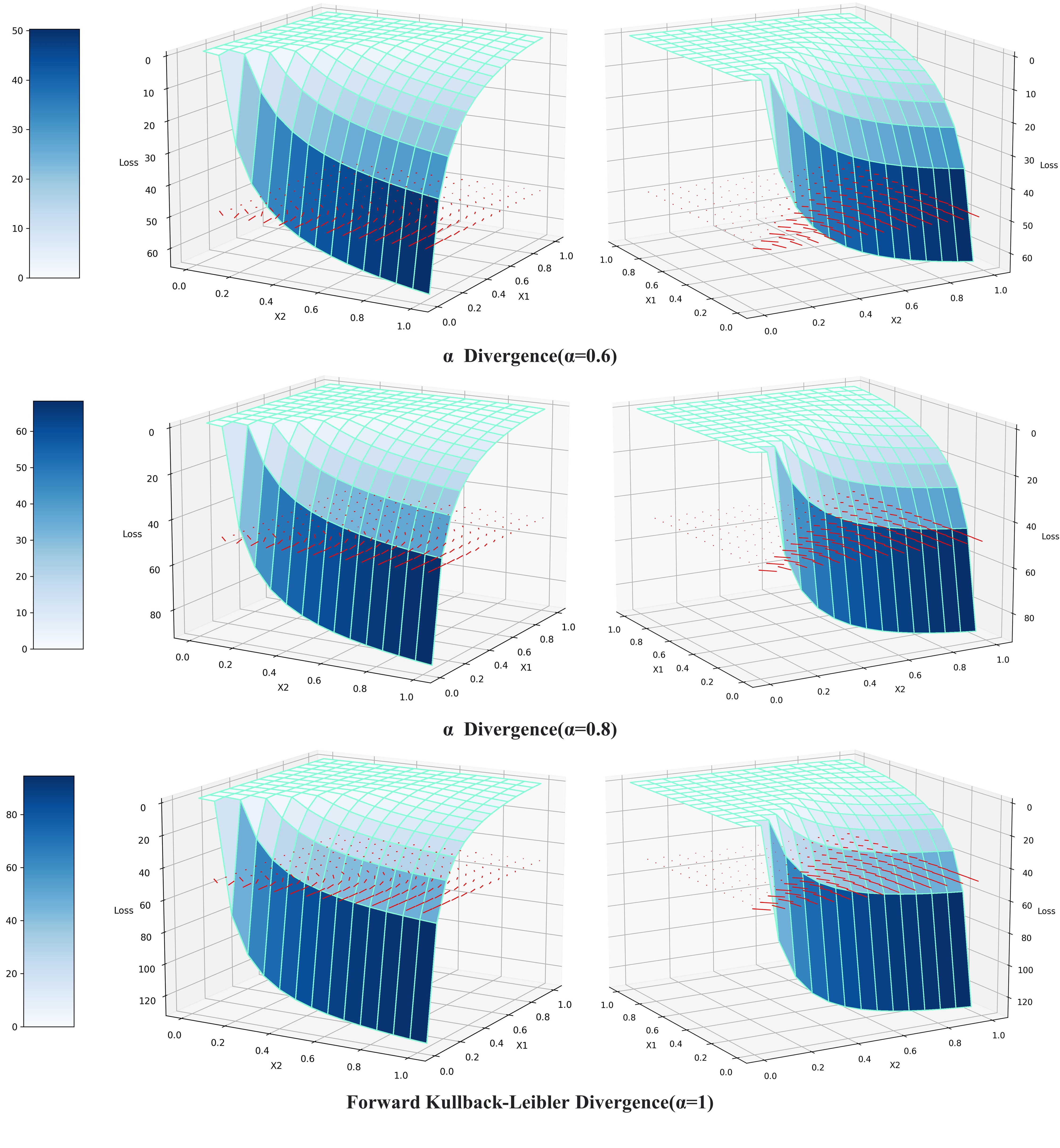
Figure 2: Landscapes’ visualization of alignment objective functions with different divergences from two viewing angles and gradient fields’ visualization of the corresponding loss function on the plane $Z=50$.

Appendix G Detailed Metric Description

G.1 Alignment Performance Metric.

In this paper, we utilize five metrics for evaluating the alignment performance. We employ the text-image CLIP score [34] to evaluate the performance of text-image alignment and the Aesthetics score [35], ImageReward [7], PickScore [6] and HPS-v2 [9] to evaluate the performance of human value alignment .

Text-Image CLIP score. The Text-Image CLIP score serves as a quantitative measure for evaluating the likeness between text-image pairs. CLIP Score is fundamentally based on the CLIP model, which transforms input text and images into distinct text and image vectors, followed by calculation of the dot product of these vectors. Foundational aim of the CLIP model is to cultivate versatile multimodal representations, free from specialized domain expertise, through the integration of linguistic indicators and visual data. Training approach of CLIP model mainly hinges on contrastive learning, where the system partitions the incoming text-image pairs into two categories: one cluster includes similar pairs to the input, whereas the other assembles dissimilar pairs. The model then learns representations of these inputs, with the objective to increment similarity within matching pairs while reducing it between non-matching pairs. Benefiting from its pre-training strategy, it enables the extraction of significant image and text features from vast unsupervised datasets. The CLIP model and CLIP score has demonstrated commendable performance across a wide range of tasks, encompassing image classification, semantic segmentation, image generation, object localization, video interpretation, and so on.

Aesthetics score. The LAION Aesthetics Predictor is utilized to estimate an image’s aesthetic score, quantifying the mean human appreciation for its visual appeal. It leverages a neural network architecture (MLP) that takes CLIP embeddings as inputs to ascertain the average preference level for the image. Each image is assigned a score on the scale of 0 to 10, with 0 signifying the least visually attractive and 10 denoting the highest level of visual appeal.

ImageReward. ImageReward, leveraging a structure that combines ViT-L for image encoding and a 12-layer Transformer for text encoding, tackles the challenges of text-to-image generation to some extent, especially regarding the quality of pre-training data, which are plagued by noise and a skewed distribution that doesn’t match the data users input in prompts. Notably, as a zero-shot evaluation tool, ImageReward often aligns with human judgments, demonstrating the capability to make nuanced quality comparisons between individual samples.

PickScore. A comprehensive, natural dataset, dubbed "Pick-a-Pic," is compiled and utilizing the dataset, an advanced scoring function, namely "PickScore", is built. "PickScore" excels in assessing generated images against prompts, surpassing not only machine learning models but also expert human evaluations. Its utility spans multiple domains such as model evaluation, image generation enhancement, text-to-image dataset refinement, and the optimization of text-to-image models through methodologies such as Reinforcement Learning Human Feedback (RLHF). PickScore follows the architecture of CLIP; provided a prompt $x$ and an image $y$, PickScore $s$ calculates a real number through the representation of $x$ with a text encoder and $y$ with an image encoder as two $d$-dimensional vectors, and subsequently returns their inner product:

$$score(x,y)=\mathrm{E}_{\text{txt}}(x)\cdot\mathrm{E}_{\text{img}}(y)\cdot T$$

where $T$ is the learned temperature parameter of CLIP.

HPS-v2. Human Preference Dataset v2 (HPD-v2) encapsulates human preferences for images sourced from a multitude of platforms. It consists of 798,090 individual human preference choices for 433,760 paired image comparisons. The dataset has been taken care to deliberately collect the text prompts and images to minimize potential biases, a common pitfall in previous datasets. Whereafter, through fine-tuning the CLIP model on HPD-v2, the Human Preference Score v2 (HPS-v2) is derived, a scoring model that can more accurately gauge human preferences for generated images. HPS-v2 has been shown to generalize more effectively than earlier metrics across a variety of image datasets, and it is responsive to algorithmic improvements of text-to-image generative models.

G.2 Generation Diversity Metric

In this work, we utilize eight metrics for comprehensively evaluating generation diversity from diverse aspects: Image-Image CLIP score [34], Image Entropy (Entropy 1D and Entropy 2D) [67], LPIPS [37], RMSE [68], PSNR [69], SSIM [69], FSIM [36].

Image-Image CLIP score. Text-Image CLIP score and Image-Image CLIP score are both grounded in the evaluation of high-dimensional embeddings produced by the CLIP model. Similarly, the Image-Image CLIP score functions as an efficacious metric for evaluating the structural congruity between images, thereby enabling assessments of images’ similarity. Hence, we select Image-Image CLIP score as an indicator for the diversity of images produced by the trained diffusion model: a diminutive CLIP score between two generated images signifies a pronounced disparity, implying that the model demonstrates a heightened capacity for generating diverse content.

Image Entropy (Entropy 1D and Entropy 2D). Image Entropy is a statistical metric employed to evaluate the information content and complexity within an image. It quantifies the average information per pixel, with higher entropy values signaling a greater diversity and richness in the image’s information content. One-dimensional image entropy (Entropy 1D) quantifies the information encapsulated within the distribution’s clustering properties of gray levels:

$$H_{1d}=\sum\limits_{i=0}^{255}P_{i}\log P_{i}$$

where $P_{i}$ presents the proportion of pixels in the image with gray level value $i$.

The one-dimensional image entropy (Entropy 1D) successfully captures the aggregation properties of gray level distribution, yet neglects spatial attributes. To rectify this discrepancy, supplementary feature metrics are incorporated, which, in conjunction with the one-dimensional entropy, serve as the cornerstone for the evolution of two-dimensional image entropy (Entropy 2D). Such augmentation facilitates a more holistic evaluation that merges both spatial and distributional data within an image. The neighborhood gray level mean, when chosen as a spatial feature quantity in conjunction with the pixel gray levels, constitutes a feature tuple denoted as $(i,j)$:

$$P_{i,j}=\frac{f(i,j)}{N^{2}}$$

where $i$ is the gray value of the pixel, and $j$ is the mean gray value of its neighborhood; $f(i,j)$ is the occurrence frequency of characteristic binary $(i,j)$ and $N$ is the dimension of the image. Then the two-dimensional image entropy (Entropy 2D) can be defined as:

$$H_{2d}=\sum\limits_{i=0}^{255}\sum\limits_{j=0}^{255}P_{ij}\log P_{ij}$$

LPIPS. Learned Perceptual Image Patch Similarity (LPIPS) is a deep learning-based metric designed for assessing image similarity, which is calculated based on features output by a deep convolutional neural network (AlexNet in our work). Utilizing the feature representations learned by a deep neural network, which is capable of capturing details of human visual perception such as texture, color, and structure, the computation of perceptual similarity between two images can be conducted. Firstly, pre-trained deep neural networks, notably those like AlexNet [70] or VGG [71], are employed to extract features from input images. The outputs from the network’s intermediate layers are then typically utilized, as they encapsulate a spectrum of abstract features, spanning from rudimentary edge and texture details to more sophisticated representations of objects and scenes, denoted as $\hat{y_{1}^{i}}$, $\hat{y_{2}^{i}}$ $\in\mathbb{R}^{H_{l}\times W_{l}\times C_{l}}$. Subsequently, the distances between extracted features in the feature space can be calculated:

$$d(y_{1},y_{2})=\sum\limits_{l}\frac{1}{H_{l}W_{l}}\sum\limits_{h,w}\|w_{l}\odot(\hat{y_{1}^{i}}-\hat{y_{2}^{i}})\|_{2}^{2}$$

and converted into a comprehensible similarity score by standardizing them to the range of 0 to 1. For our evaluation, LPIPS is selected as a metric; a lower score indicates a higher similarity between images, while a higher score suggests greater diversity or disparity between them.

RMSE. Root Mean Square Error (RMSE) is a statistical metric that primarily employed in statistical analysis and machine learning disciplines, serving as a benchmark for gauging the accuracy of predictions. In our scenario, we utilize the RMSE as a criterion to measure the pixel-level differences between pairs of generated images. Such pixel-level variance can be considered as an indicator of the images’ diversity, thereby offering a quantifiable assessment of the generated images’ diversity:

$$RMSE=\sqrt{\frac{1}{L\times W}\sum\limits_{i=1}^{L\times W}(p_{i}-q_{i})^{2}}$$

where $L$ is the length of the image, $W$ is the width of the image; $p_{i}$ and $q_{i}$ are $i$-th pixels of two generated images.

PNSR. Peak Signal-to-Noise Ratio (PSNR), a prevalent metric in image processing and compression, quantitatively assesses the discrepancy between an original image and its modified counterpart. This metric, typically reported in decibels (dB), is characterized by a higher value indicative of a diminished difference between the two images, effectively serving as a metric for evaluating the diversity of generated images:

$$PSNR=10\log_{10}\Big{(}\frac{Max^{2}}{MSE}\Big{)}$$

where $Max$ denotes the maximum pixel value that an image attain, $MSE$ denotes the mean squared error between two images.

SSIM. Structural Similarity Index Measure (SSIM) is a metric designed to assess the likeness between images by emulating the human visual system’s perception of image quality. Traditional metrics (e.g. RMSE, PNSR, Image Entropy) usually focus on disparities in pixel values, whereas SSIM incorporates the structural aspects of images for evaluation. It is often executed from three aspects: luminance similarity, contrast similarity, and structural similarity - on a scale from 0 to 1:

$$\begin{split}l(x,y)&=\frac{2\mu_{x}\mu_{y}+c_{1}}{\mu_{x}^{2}+\mu_{y}^{2}+c_{1}};\\ c(x,y)&=\frac{2\sigma_{x}\sigma_{y}+c_{2}}{\sigma_{x}^{2}+\sigma_{y}^{2}+c_{2}};\\ s(x,y)&=\frac{\sigma_{xy}+c_{3}}{\sigma_{x}\sigma_{y}+c_{3}}\end{split}$$

where $\mu_{x}$ and $\mu_{y}$ are means of $x$ and $y$; $\sigma_{x}$ and $\sigma_{y}$ are variances of $x$ and $y$, respectively; and $\sigma_{xy}$ is the covariance of $x$ and $y$. SSIM calculates similarity between two images across these three dimensions, providing an overall similarity index ranging from 0 to 1. The closer the value is to 1, the more similar the two images are:

$$SSIM(x,y)=\left[l(x,y)^{\alpha}\cdot c(x,y)^{\beta}\cdot s(x,y)^{\gamma}\right]$$

In typical situations, $\alpha$, $\beta$ and $\gamma$ are all set to 1.

FSIM. Feature Similarity Index Measure (FSIM) utilizes feature similarity for assessment. The Human Visual System (HVS) bases its perception on essential visual attributes, and the phase congruency (PC) feature excels in depicting local structures. Remarkably, PC’s resilience to changes in the image context guarantees the stability of feature extraction. Nonetheless, it’s recognized that modifications in the image can influence visual perception. Therefore, to augment the comprehensive analysis, gradient features, particularly gradient magnitude (GM), are incorporated. Consequently, in FSIM, both PC and GM features collaborate to serve complementary roles, synergistically capturing a holistic evaluation. For two images, the calculations for $PC1$, $GM1$, $PC2$, and $GM2$ are firstly performed. Subsequently, compute the similarity for $PC$ and for $GM$ as follows:

$$\begin{split}S_{PC}(\mathrm{x})&=\frac{2PC_{1}(\mathrm{x})\cdot PC_{2}(\mathrm{x})+T_{1}}{PC_{1}(\mathrm{x})^{2}+PC_{2}(\mathrm{x})^{2}+T_{1}};\\ S_{GM}(\mathrm{x})&=\frac{2GM_{1}(\mathrm{x})\cdot GM_{2}(x)+T_{2}}{GM_{1}(x)^{2}+GM_{2}(x)^{2}+T_{2}}.\end{split}$$

Furthermore, the similarity expressed by fusion of PC and GM can be given as:

$$S_{L}(\mathrm{x})=[S_{PC}(\mathrm{x})]^{\alpha}\cdot[S_{GM}(\mathrm{x})]^{\beta}$$

Finally, the calculation of FSIM is described as follows:

$$FSIM=\frac{\sum_{\mathrm{x}\in\Omega}S_{L}(\mathrm{x})\cdot PC_{m}(\mathrm{x})}{\sum_{\mathrm{x}\in\Omega}PC_{m}(\mathrm{x})}$$

Appendix H Further Larger-Scale Evaluation

To further demonstrate the persuasiveness of our conclusions, we conduct a larger-scale evaluation on the aligned models. We firstly employed the parti-prompts [72] training dataset, which consists of 1632 prompts. Subsequently, the entire HPS-v2 [9] training set, which consists of 3,200 prompts, is employed. Combining the generated images from these sets together, we report the evaluation results on all 4832 prompts in Table 2 (alignment performance) and Table 3 (generation diversity), including the mean and standard deviation. The results obtained are similar to that in the main paper. Jensen-Shannon divergence exhibits the best alignment performance and suboptimal generation diversity, achieving the best trade-off.

Model		Text-Image CLIP score $\uparrow$	Aesthetics Score $\uparrow$	ImageReward $\uparrow$	Pickscore $\uparrow$	HPS-V2 $\uparrow$
Original Model		0.343 $\pm$ 0.054	5.575 $\pm$ 0.556	0.231 $\pm$ 1.047	21.059 $\pm$ 1.216	27.082 $\pm$ 1.541
Reverse KL Divergence		0.353 $\pm$ 0.053	5.698 $\pm$ 0.534	0.661 $\pm$ 0.940	21.682 $\pm$ 1.194	27.907 $\pm$ 1.519
$\alpha$-Divergence	$\alpha$=0.2	0.352 $\pm$ 0.054	5.712 $\pm$ 0.527	0.627 $\pm$ 0.962	21.581 $\pm$ 1.200	27.953 $\pm$ 1.543
	$\alpha$=0.4	0.351 $\pm$ 0.053	5.659 $\pm$ 0.519	0.626 $\pm$ 0.957	21.611 $\pm$ 1.205	27.840 $\pm$ 1.504
	$\alpha$=0.6	0.349 $\pm$ 0.053	5.666 $\pm$ 0.509	0.569 $\pm$ 0.971	21.456 $\pm$ 1.205	27.831 $\pm$ 1.513
	$\alpha$=0.8	0.351 $\pm$ 0.054	5.701 $\pm$ 0.537	0.598 $\pm$ 0.969	21.555 $\pm$ 1.195	27.786 $\pm$ 1.510
Forward KL Divergence		0.353 $\pm$ 0.054	5.735 $\pm$ 0.524	0.626 $\pm$ 0.952	21.640 $\pm$ 1.184	27.941 $\pm$ 1.510
Jensen-Shannon Divergence		0.352 $\pm$ 0.053	5.765 $\pm$ 0.513	0.672 $\pm$ 0.942	21.708 $\pm$ 1.194	27.954 $\pm$ 1.502

Table 4: Evaluations of the alignment performance with larger-scale experiments, where the Text-Image CLIP score evaluates image-text alignment performance, and the remaining four metrics evaluate human value alignment performance.

Model		Image-Image CLIP score $\downarrow$	Entropy 1D $\uparrow$	Entropy 2D $\uparrow$	LPIPS $\uparrow$
Original Model		0.8096 $\pm$ 0.0982	3.8279 $\pm$ 0.2675	7.5427 $\pm$ 0.5896	0.3002 $\pm$ 0.0404
Reverse KL Divergence		0.8491 $\pm$ 0.0891	3.9519 $\pm$ 0.1578	7.7858 $\pm$ 0.3904	0.2957 $\pm$ 0.0349
$\alpha$-Divergence	$\alpha=$0.2	0.8420 $\pm$ 0.0887	3.9231 $\pm$ 0.1743	7.8985 $\pm$ 0.3214	0.3096 $\pm$ 0.0321
	$\alpha=$0.4	0.8471 $\pm$ 0.0892	3.9689 $\pm$ 0.1564	7.7860 $\pm$ 0.3721	0.2995 $\pm$ 0.0348
	$\alpha=$0.6	0.8472 $\pm$ 0.0881	3.9216 $\pm$ 0.1932	7.7592 $\pm$ 0.4400	0.3132 $\pm$ 0.0140
	$\alpha=$0.8	0.8423 $\pm$ 0.0795	3.9448 $\pm$ 0.1851	7.7059 $\pm$ 0.4409	0.3030 $\pm$ 0.0363
Forward KL Divergence		0.8505 $\pm$ 0.0876	3.9409 $\pm$ 0.1639	7.7315 $\pm$ 0.3868	0.3004 $\pm$ 0.0346
Jensen-Shannon Divergence		0.8503 $\pm$ 0.0885	3.9532 $\pm$ 0.1569	7.8239 $\pm$ 0.3928	0.3036 $\pm$ 0.0358

Model		RMSE $\uparrow$	PSNR $\downarrow$	SSIM $\downarrow$	FSIM $\downarrow$
Original Model		0.0133 $\pm$ 0.0028	37.660 $\pm$ 1.879	0.8819 $\pm$ 0.0380	0.3779 $\pm$ 0.0227
Reverse KL Divergence		0.0154 $\pm$ 0.0027	36.360 $\pm$ 1.587	0.8521 $\pm$ 0.0374	0.3800 $\pm$ 0.0185
$\alpha$-Divergence	$\alpha=$0.2	0.0176 $\pm$ 0.0025	35.192 $\pm$ 1.280	0.8354 $\pm$ 0.0350	0.3757 $\pm$ 0.0182
	$\alpha=$0.4	0.0155 $\pm$ 0.0026	36.317 $\pm$ 1.489	0.8535 $\pm$ 0.0357	0.3806 $\pm$ 0.0184
	$\alpha=$0.6	0.0166 $\pm$ 0.0027	35.708 $\pm$ 1.488	0.8371 $\pm$ 0.0348	0.3765 $\pm$ 0.0212
	$\alpha=$0.8	0.0155 $\pm$ 0.0028	36.327 $\pm$ 1.646	0.8528 $\pm$ 0.0383	0.3789 $\pm$ 0.0210
Forward KL Divergence		0.0157 $\pm$ 0.0026	36.133 $\pm$ 1.536	0.8475 $\pm$ 0.0366	0.3763 $\pm$ 0.0194
Jensen-Shannon Divergence		0.0158 $\pm$ 0.0026	36.054 $\pm$ 1.511	0.8450 $\pm$ 0.0363	0.3798 $\pm$ 0.0202

Table 5: Evaluations of the generation diversity with larger-scale experiments. The metrics originally utilized for evaluating image similarity exhibit an opposite property when evaluating generation diversity.

Appendix I Qualitative Comparison of Alignment with Diverse Divergence

References

- Podell et al. [2024] Dustin Podell, Zion English, Kyle Lacey, Andreas Blattmann, Tim Dockhorn, Jonas Müller, Joe Penna, and Robin Rombach. Sdxl: Improving latent diffusion models for high-resolution image synthesis. In The Twelfth International Conference on Learning Representations, 2024.
- Esser et al. [2024] Patrick Esser, Sumith Kulal, Andreas Blattmann, Rahim Entezari, Jonas Müller, Harry Saini, Yam Levi, Dominik Lorenz, Axel Sauer, Frederic Boesel, et al. Scaling rectified flow transformers for high-resolution image synthesis. In Forty-first International Conference on Machine Learning, 2024.
- Li et al. [2024a] Tianhong Li, Yonglong Tian, He Li, Mingyang Deng, and Kaiming He. Autoregressive image generation without vector quantization. arXiv preprint arXiv:2406.11838, 2024a.
- Betker et al. [2023] James Betker, Gabriel Goh, Li Jing, Tim Brooks, Jianfeng Wang, Linjie Li, Long Ouyang, Juntang Zhuang, Joyce Lee, Yufei Guo, et al. Improving image generation with better captions. Computer Science. https://cdn. openai. com/papers/dall-e-3. pdf, 2(3):8, 2023.
- Liu et al. [2021] Xiao Liu, Fanjin Zhang, Zhenyu Hou, Li Mian, Zhaoyu Wang, Jing Zhang, and Jie Tang. Self-supervised learning: Generative or contrastive. IEEE transactions on knowledge and data engineering, 35(1):857–876, 2021.
- Kirstain et al. [2023] Yuval Kirstain, Adam Polyak, Uriel Singer, Shahbuland Matiana, Joe Penna, and Omer Levy. Pick-a-pic: An open dataset of user preferences for text-to-image generation. Advances in Neural Information Processing Systems, 36:36652–36663, 2023.
- Xu et al. [2024] Jiazheng Xu, Xiao Liu, Yuchen Wu, Yuxuan Tong, Qinkai Li, Ming Ding, Jie Tang, and Yuxiao Dong. Imagereward: Learning and evaluating human preferences for text-to-image generation. Advances in Neural Information Processing Systems, 36, 2024.
- Black et al. [2024] Kevin Black, Michael Janner, Yilun Du, Ilya Kostrikov, and Sergey Levine. Training diffusion models with reinforcement learning. In The Twelfth International Conference on Learning Representations, 2024.
- Wu et al. [2023] Xiaoshi Wu, Yiming Hao, Keqiang Sun, Yixiong Chen, Feng Zhu, Rui Zhao, and Hongsheng Li. Human preference score v2: A solid benchmark for evaluating human preferences of text-to-image synthesis. arXiv preprint arXiv:2306.09341, 2023.
- Bradley and Terry [1952] Ralph Allan Bradley and Milton E. Terry. Rank analysis of incomplete block designs: I. the method of paired comparisons. Biometrika, 39(3/4):324–345, 1952. ISSN 00063444.
- Rafailov et al. [2023] Rafael Rafailov, Archit Sharma, Eric Mitchell, Stefano Ermon, Christopher D Manning, and Chelsea Finn. Direct preference optimization: your language model is secretly a reward model. In Proceedings of the 37th International Conference on Neural Information Processing Systems, pages 53728–53741, 2023.
- Wallace et al. [2024] Bram Wallace, Meihua Dang, Rafael Rafailov, Linqi Zhou, Aaron Lou, Senthil Purushwalkam, Stefano Ermon, Caiming Xiong, Shafiq Joty, and Nikhil Naik. Diffusion model alignment using direct preference optimization. In Proceedings of the IEEE/CVF Conference on Computer Vision and Pattern Recognition, pages 8228–8238, 2024.
- Yang et al. [2024a] Kai Yang, Jian Tao, Jiafei Lyu, Chunjiang Ge, Jiaxin Chen, Weihan Shen, Xiaolong Zhu, and Xiu Li. Using human feedback to fine-tune diffusion models without any reward model. In Proceedings of the IEEE/CVF Conference on Computer Vision and Pattern Recognition, pages 8941–8951, 2024a.
- Liang et al. [2024] Zhanhao Liang, Yuhui Yuan, Shuyang Gu, Bohan Chen, Tiankai Hang, Ji Li, and Liang Zheng. Step-aware preference optimization: Aligning preference with denoising performance at each step. arXiv preprint arXiv:2406.04314, 2024.
- Gambashidze et al. [2024] Alexander Gambashidze, Anton Kulikov, Yuriy Sosnin, and Ilya Makarov. Aligning diffusion models with noise-conditioned perception. arXiv preprint arXiv:2406.17636, 2024.
- Tang et al. [2024] Zhiwei Tang, Jiangweizhi Peng, Jiasheng Tang, Mingyi Hong, Fan Wang, and Tsung-Hui Chang. Tuning-free alignment of diffusion models with direct noise optimization. arXiv preprint arXiv:2405.18881, 2024.
- Ruiz et al. [2023] Nataniel Ruiz, Yuanzhen Li, Varun Jampani, Yael Pritch, Michael Rubinstein, and Kfir Aberman. Dreambooth: Fine tuning text-to-image diffusion models for subject-driven generation. In Proceedings of the IEEE/CVF Conference on Computer Vision and Pattern Recognition (CVPR), pages 22500–22510, June 2023.
- Wiher et al. [2022] Gian Wiher, Clara Meister, and Ryan Cotterell. On decoding strategies for neural text generators. Transactions of the Association for Computational Linguistics, 10:997–1012, 2022.
- Perez et al. [2022] Ethan Perez, Saffron Huang, Francis Song, Trevor Cai, Roman Ring, John Aslanides, Amelia Glaese, Nat McAleese, and Geoffrey Irving. Red teaming language models with language models. In Proceedings of the 2022 Conference on Empirical Methods in Natural Language Processing, pages 3419–3448, 2022.
- Go et al. [2023] Dongyoung Go, Tomasz Korbak, Germàn Kruszewski, Jos Rozen, Nahyeon Ryu, and Marc Dymetman. Aligning language models with preferences through -divergence minimization. In International Conference on Machine Learning, pages 11546–11583. PMLR, 2023.
- Wang et al. [2024] Chaoqi Wang, Yibo Jiang, Chenghao Yang, Han Liu, and Yuxin Chen. Beyond reverse kl: Generalizing direct preference optimization with diverse divergence constraints. In The Twelfth International Conference on Learning Representations, 2024.
- Rombach et al. [2022] Robin Rombach, Andreas Blattmann, Dominik Lorenz, Patrick Esser, and Björn Ommer. High-resolution image synthesis with latent diffusion models. In Proceedings of the IEEE/CVF Conference on Computer Vision and Pattern Recognition (CVPR), pages 10684–10695, June 2022.
- Yang et al. [2024b] Shentao Yang, Tianqi Chen, and Mingyuan Zhou. A dense reward view on aligning text-to-image diffusion with preference. In Forty-first International Conference on Machine Learning, 2024b.
- Li et al. [2024b] Shufan Li, Harkanwar Singh, and Aditya Grover. Popalign: Population-level alignment for fair text-to-image generation. arXiv preprint arXiv:2406.19668, 2024b.
- Li et al. [2024c] Shufan Li, Konstantinos Kallidromitis, Akash Gokul, Yusuke Kato, and Kazuki Kozuka. Aligning diffusion models by optimizing human utility. arXiv preprint arXiv:2404.04465, 2024c.
- Goodfellow et al. [2014] Ian Goodfellow, Jean Pouget-Abadie, Mehdi Mirza, Bing Xu, David Warde-Farley, Sherjil Ozair, Aaron Courville, and Yoshua Bengio. Generative adversarial nets. Advances in neural information processing systems, 27, 2014.
- Nowozin et al. [2016] Sebastian Nowozin, Botond Cseke, and Ryota Tomioka. f-gan: Training generative neural samplers using variational divergence minimization. In D. Lee, M. Sugiyama, U. Luxburg, I. Guyon, and R. Garnett, editors, Advances in Neural Information Processing Systems, volume 29. Curran Associates, Inc., 2016.
- Arjovsky et al. [2017] Martin Arjovsky, Soumith Chintala, and Léon Bottou. Wasserstein generative adversarial networks. In International conference on machine learning, pages 214–223. PMLR, 2017.
- Theis et al. [2016] L Theis, A van den Oord, and M Bethge. A note on the evaluation of generative models. In International Conference on Learning Representations (ICLR 2016), pages 1–10, 2016.
- Liese and Vajda [2006] Friedrich Liese and Igor Vajda. On divergences and informations in statistics and information theory. IEEE Transactions on Information Theory, 52(10):4394–4412, 2006.
- Hiriart-Urruty and Lemaréchal [1996] Jean-Baptiste Hiriart-Urruty and Claude Lemaréchal. Convex analysis and minimization algorithms I: Fundamentals, volume 305. Springer science & business media, 1996.
- Feng et al. [2024] Duanyu Feng, Bowen Qin, Chen Huang, Zheng Zhang, and Wenqiang Lei. Towards analyzing and understanding the limitations of dpo: A theoretical perspective. arXiv preprint arXiv:2404.04626, 2024.
- Yan et al. [2024] Yuzi Yan, Yibo Miao, Jialian Li, Yipin Zhang, Jian Xie, Zhijie Deng, and Dong Yan. 3d-properties: Identifying challenges in dpo and charting a path forward. arXiv preprint arXiv:2406.07327, 2024.
- Hessel et al. [2021] Jack Hessel, Ari Holtzman, Maxwell Forbes, Ronan Le Bras, and Yejin Choi. Clipscore: A reference-free evaluation metric for image captioning. arXiv preprint arXiv:2104.08718, 2021.
- Schuhmann et al. [2022] Christoph Schuhmann, Romain Beaumont, Richard Vencu, Cade Gordon, Ross Wightman, Mehdi Cherti, Theo Coombes, Aarush Katta, Clayton Mullis, Mitchell Wortsman, et al. Laion-5b: An open large-scale dataset for training next generation image-text models. Advances in Neural Information Processing Systems, 35:25278–25294, 2022.
- Zhang et al. [2011] Lin Zhang, Lei Zhang, Xuanqin Mou, and David Zhang. Fsim: A feature similarity index for image quality assessment. IEEE transactions on Image Processing, 20(8):2378–2386, 2011.
- Zhang et al. [2018] Richard Zhang, Phillip Isola, Alexei A Efros, Eli Shechtman, and Oliver Wang. The unreasonable effectiveness of deep features as a perceptual metric. In Proceedings of the IEEE conference on computer vision and pattern recognition, pages 586–595, 2018.
- Christiano et al. [2017] Paul F Christiano, Jan Leike, Tom Brown, Miljan Martic, Shane Legg, and Dario Amodei. Deep reinforcement learning from human preferences. Advances in neural information processing systems, 30, 2017.
- Ziegler et al. [2019] Daniel M Ziegler, Nisan Stiennon, Jeffrey Wu, Tom B Brown, Alec Radford, Dario Amodei, Paul Christiano, and Geoffrey Irving. Fine-tuning language models from human preferences. arXiv preprint arXiv:1909.08593, 2019.
- Casper et al. [2023] Stephen Casper, Xander Davies, Claudia Shi, Thomas Krendl Gilbert, Jérémy Scheurer, Javier Rando, Rachel Freedman, Tomasz Korbak, David Lindner, Pedro Freire, et al. Open problems and fundamental limitations of reinforcement learning from human feedback. Transactions on Machine Learning Research, 2023.
- Hejna III and Sadigh [2023] Donald Joseph Hejna III and Dorsa Sadigh. Few-shot preference learning for human-in-the-loop rl. In Conference on Robot Learning, pages 2014–2025. PMLR, 2023.
- Bai et al. [2022] Yuntao Bai, Andy Jones, Kamal Ndousse, Amanda Askell, Anna Chen, Nova DasSarma, Dawn Drain, Stanislav Fort, Deep Ganguli, Tom Henighan, et al. Training a helpful and harmless assistant with reinforcement learning from human feedback. arXiv preprint arXiv:2204.05862, 2022.
- Achiam et al. [2023] Josh Achiam, Steven Adler, Sandhini Agarwal, Lama Ahmad, Ilge Akkaya, Florencia Leoni Aleman, Diogo Almeida, Janko Altenschmidt, Sam Altman, Shyamal Anadkat, et al. Gpt-4 technical report. arXiv preprint arXiv:2303.08774, 2023.
- Touvron et al. [2023] Hugo Touvron, Louis Martin, Kevin Stone, Peter Albert, Amjad Almahairi, Yasmine Babaei, Nikolay Bashlykov, Soumya Batra, Prajjwal Bhargava, Shruti Bhosale, et al. Llama 2: Open foundation and fine-tuned chat models. arXiv preprint arXiv:2307.09288, 2023.
- Team et al. [2024] Gemma Team, Thomas Mesnard, Cassidy Hardin, Robert Dadashi, Surya Bhupatiraju, Shreya Pathak, Laurent Sifre, Morgane Rivière, Mihir Sanjay Kale, Juliette Love, et al. Gemma: Open models based on gemini research and technology. arXiv preprint arXiv:2403.08295, 2024.
- Schulman et al. [2017] John Schulman, Filip Wolski, Prafulla Dhariwal, Alec Radford, and Oleg Klimov. Proximal policy optimization algorithms, 2017.
- Ramamurthy et al. [2023] Rajkumar Ramamurthy, Prithviraj Ammanabrolu, Kianté Brantley, Jack Hessel, Rafet Sifa, Christian Bauckhage, Hannaneh Hajishirzi, and Yejin Choi. Is reinforcement learning (not) for natural language processing: Benchmarks, baselines, and building blocks for natural language policy optimization. In The Eleventh International Conference on Learning Representations, 2023.
- Skalse et al. [2022] Joar Skalse, Nikolaus Howe, Dmitrii Krasheninnikov, and David Krueger. Defining and characterizing reward gaming. Advances in Neural Information Processing Systems, 35:9460–9471, 2022.
- Gao et al. [2023] Leo Gao, John Schulman, and Jacob Hilton. Scaling laws for reward model overoptimization. In International Conference on Machine Learning, pages 10835–10866. PMLR, 2023.
- Sohl-Dickstein et al. [2015] Jascha Sohl-Dickstein, Eric Weiss, Niru Maheswaranathan, and Surya Ganguli. Deep unsupervised learning using nonequilibrium thermodynamics. In International conference on machine learning, pages 2256–2265. PMLR, 2015.
- Ho et al. [2020] Jonathan Ho, Ajay Jain, and Pieter Abbeel. Denoising diffusion probabilistic models. Advances in neural information processing systems, 33:6840–6851, 2020.
- Zhang et al. [2023a] Tianyi Zhang, Zheng Wang, Jing Huang, Mohiuddin Muhammad Tasnim, and Wei Shi. A survey of diffusion based image generation models: Issues and their solutions. arXiv preprint arXiv:2308.13142, 2023a.
- Liao et al. [2024] Huan Liao, Haonan Han, Kai Yang, Tianjiao Du, Rui Yang, Zunnan Xu, Qinmei Xu, Jingquan Liu, Jiasheng Lu, and Xiu Li. Baton: Aligning text-to-audio model with human preference feedback. arXiv preprint arXiv:2402.00744, 2024.
- Xing et al. [2023] Zhen Xing, Qijun Feng, Haoran Chen, Qi Dai, Han Hu, Hang Xu, Zuxuan Wu, and Yu-Gang Jiang. A survey on video diffusion models. arXiv preprint arXiv:2310.10647, 2023.
- Chan et al. [2023] Eric R Chan, Koki Nagano, Matthew A Chan, Alexander W Bergman, Jeong Joon Park, Axel Levy, Miika Aittala, Shalini De Mello, Tero Karras, and Gordon Wetzstein. Generative novel view synthesis with 3d-aware diffusion models. In Proceedings of the IEEE/CVF International Conference on Computer Vision, pages 4217–4229, 2023.
- Kapelyukh et al. [2023] Ivan Kapelyukh, Vitalis Vosylius, and Edward Johns. Dall-e-bot: Introducing web-scale diffusion models to robotics. IEEE Robotics and Automation Letters, 8(7):3956–3963, 2023.
- Raffel et al. [2020] Colin Raffel, Noam Shazeer, Adam Roberts, Katherine Lee, Sharan Narang, Michael Matena, Yanqi Zhou, Wei Li, and Peter J Liu. Exploring the limits of transfer learning with a unified text-to-text transformer. Journal of machine learning research, 21(140):1–67, 2020.
- Radford et al. [2021] Alec Radford, Jong Wook Kim, Chris Hallacy, Aditya Ramesh, Gabriel Goh, Sandhini Agarwal, Girish Sastry, Amanda Askell, Pamela Mishkin, Jack Clark, et al. Learning transferable visual models from natural language supervision. In International conference on machine learning, pages 8748–8763. PMLR, 2021.
- Ramesh et al. [2021] Aditya Ramesh, Mikhail Pavlov, Gabriel Goh, Scott Gray, Chelsea Voss, Alec Radford, Mark Chen, and Ilya Sutskever. Zero-shot text-to-image generation. In International conference on machine learning, pages 8821–8831. Pmlr, 2021.
- Zhang et al. [2023b] Lvmin Zhang, Anyi Rao, and Maneesh Agrawala. Adding conditional control to text-to-image diffusion models. In Proceedings of the IEEE/CVF International Conference on Computer Vision, pages 3836–3847, 2023b.
- Liu et al. [2022] Nan Liu, Shuang Li, Yilun Du, Antonio Torralba, and Joshua B Tenenbaum. Compositional visual generation with composable diffusion models. In European Conference on Computer Vision, pages 423–439. Springer, 2022.
- Feng et al. [2023] Weixi Feng, Xuehai He, Tsu-Jui Fu, Varun Jampani, Arjun Reddy Akula, Pradyumna Narayana, Sugato Basu, Xin Eric Wang, and William Yang Wang. Training-free structured diffusion guidance for compositional text-to-image synthesis. In The Eleventh International Conference on Learning Representations, 2023.
- Lee et al. [2023] Kimin Lee, Hao Liu, Moonkyung Ryu, Olivia Watkins, Yuqing Du, Craig Boutilier, Pieter Abbeel, Mohammad Ghavamzadeh, and Shixiang Shane Gu. Aligning text-to-image models using human feedback. arXiv preprint arXiv:2302.12192, 2023.
- Wallace et al. [2023] Bram Wallace, Akash Gokul, Stefano Ermon, and Nikhil Naik. End-to-end diffusion latent optimization improves classifier guidance. In Proceedings of the IEEE/CVF International Conference on Computer Vision, pages 7280–7290, 2023.
- Clark et al. [2024] Kevin Clark, Paul Vicol, Kevin Swersky, and David J Fleet. Directly fine-tuning diffusion models on differentiable rewards. In The Twelfth International Conference on Learning Representations, 2024.
- Fan et al. [2024] Ying Fan, Olivia Watkins, Yuqing Du, Hao Liu, Moonkyung Ryu, Craig Boutilier, Pieter Abbeel, Mohammad Ghavamzadeh, Kangwook Lee, and Kimin Lee. Reinforcement learning for fine-tuning text-to-image diffusion models. Advances in Neural Information Processing Systems, 36, 2024.
- Sparavigna [2019] Amelia Carolina Sparavigna. Entropy in image analysis, 2019.
- Willmott and Matsuura [2005] Cort J. Willmott and Kenji Matsuura. Advantages of the mean absolute error (mae) over the root mean square error (rmse) in assessing average model performance. Climate Research, 30:79–82, 2005. URL https://api.semanticscholar.org/CorpusID:120556606.
- Horé and Ziou [2010] Alain Horé and Djemel Ziou. Image quality metrics: Psnr vs. ssim. In 2010 20th International Conference on Pattern Recognition, pages 2366–2369, Aug 2010. doi: 10.1109/ICPR.2010.579.
- Krizhevsky et al. [2012] Alex Krizhevsky, Ilya Sutskever, and Geoffrey E Hinton. Imagenet classification with deep convolutional neural networks. In F. Pereira, C.J. Burges, L. Bottou, and K.Q. Weinberger, editors, Advances in Neural Information Processing Systems, volume 25. Curran Associates, Inc., 2012. URL https://proceedings.neurips.cc/paper_files/paper/2012/file/c399862d3b9d6b76c8436e924a68c45b-Paper.pdf.
- Simonyan [2014] Karen Simonyan. Very deep convolutional networks for large-scale image recognition. arXiv preprint arXiv:1409.1556, 2014.
- Yu et al. [2022] Jiahui Yu, Yuanzhong Xu, Jing Yu Koh, Thang Luong, Gunjan Baid, Zirui Wang, Vijay Vasudevan, Alexander Ku, Yinfei Yang, Burcu Karagol Ayan, et al. Scaling autoregressive models for content-rich text-to-image generation. Transactions on Machine Learning Research, 2022.