Feasibility Study of Curvature Effect in Flexible Antenna Arrays for 2-Dimensional Beam Alignment of 6G Wireless Systems

Abstract

This article investigates the influential role of flexible antenna array curvature on the performance of 6G communication systems with carrier frequencies above 100 GHz. It is demonstrated that the curvature of flexible antenna arrays can be leveraged for 2-dimensional beam alignment in phased arrays with relatively small insertion loss. The effect of antenna array bending on the radiation properties such as gain and antenna impedance are analytically studied and simulated for a 4$\times$4 microstrip patch antenna array operating between 97.5-102.5 GHz. Moreover, the deployment of this flexible antenna array in conjunction with state-of-the-art flexible board packaging techniques is examined for 6G wireless transceivers based on 65nm CMOS technology and simulated for three variants of quadrature amplitude modulation (4QAM, 16 QAM, and 64 QAM). The communication performance in terms of signal-to-noise ratio (SNR) and bit error rate (BER) is evaluated using analytical derivations and simulation results which exhibit a relatively close match.

I Introduction

In light of advances in semiconductor technologies, the demand for higher data rates in communication systems and higher resolution in imaging and radar technologies is continuously growing [1]. By increasing the carrier frequency and signal bandwidth, the communication data rate and sensing resolution can increase, respectively [2].

To mitigate the propagation loss at mm-wave and sub-terahertz frequencies, high-gain power amplifiers on the CMOS circuit as well as high-gain and efficient antenna elements for the wireless signal transmission/reception are necessary.

The antenna elements for CMOS-based mm-wave transceivers can be either on-chip [3] or off-chip [4, 5]. To mitigate the limited gain and efficiency of on-chip antennas, off-chip antennas with superior efficiency and bandwidth have been demonstrated in the literature [4] along with low-loss interface technologies [6]. To extend the angular coverage of mm-wave systems, phased-array architectures are adopted. For mm-wave phased array systems, one major challenge is the beam alignment between transmitter (TX) and receiver (RX) channels, which is currently done by various phase shifting techniques. A common challenge among all the techniques is the design of low-power broadband phase-shifting/time-delay circuits with relatively small insertion loss [7]. Not only does the dynamic range of these phase shifters impact the beam alignment range of phased array systems, but they also consume considerable power when realized by active devices[8]. By adopting the mm-wave phased arrays for multiple input multiple output communication systems, phase shifters in each TX and RX channel should be tuned in order to achieve beam alignment and extended coverage [9]. However, as shown in Fig. 1(a) the beam alignment of these conventional linear array systems is limited by the phase shifters.

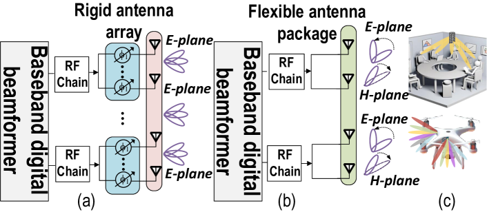
Figure 1: (a) conventional hybrid beamforming architecture with 1-D beam alignment, (b) proposed 2-D beam alignment architecture by extended aerial coverage, (c) target applications to deploy the flexible antenna arrays.

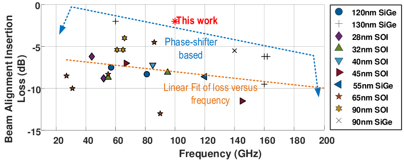
Figure 2: The insertion loss of beam alignment based on phase shifters compared to the proposed flexible antenna.

Building on top of recent advances in fabrication of mm-wave antenna elements above 100 GHz using flexible printed circuit technologies [4], this paper delves into the analysis, simulation, and investigation of extended 2-D beam steering by deploying the curvature of flexible antenna arrays as shown in Fig. 1(b) for indoor and outdoor applications, Fig. 1(c). The main objective of the proposed design is to get rid of the unwanted insertion loss of phase shifters in mm-wave phased arrays (see Fig. 2) and achieve beam alignment with substantially reduced insertion loss. Using the same technology that was deployed in [4] and by introducing novel packaging solutions, the beam rotation in a 4$\times$4 planar microstrip patch antenna array at 97.5-102.5 GHz is analytically studied in Section II where the relationship between the antenna parameters and the degree of folding is presented. In Section III the presented antenna array is deployed in a 6G wireless transceiver based on a 65-nm CMOS transciever and simulations are conducted and compared with analytical derivations for the performance of the 6G systems. The paper is concluded in Section IV.

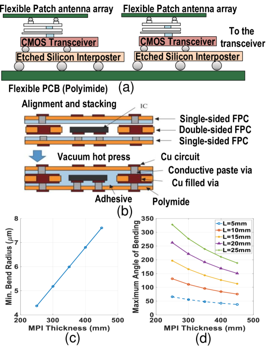
Figure 3: (a) heterogeneous package comprising CMOS chipsets and antenna on FPC, (b) buried chip in FPC package. Measured values of (c) bend radius for various substrate thickness, and (d) board flexibility maximum angle vs. its dimensions.

II Flexible Antenna Design and Packaging

To design a multiple-input multiple-output array, the packaging of the antenna and system-on-chip (SOC), the main board and interposer should be considered. We examine two multi-level integration schemes that are custom designed for this specific application and are shown in Fig. 3. In Fig. 3(a) each CMOS transceiver chip and the corresponding interposer will be placed between two flexible layers (modified polyimide material with $\epsilon_{r}=3.1$ and loss tangent of 0.003) at the bottom and top. This scheme is preferred for MIMO systems. In Fig. 3(b), the buried chip inside the flexible printed circuit board (FPC) materials is proposed with reduced insertion loss for the interface between the board and the chip. Both technologies have been experimentally validated and according to our recent measurements in Fig. 3(c,d), for various thicknesses of the substrate (MPI), the minimum bend radius of few mm is achievable. Moreover, the maximum bend angle of the board increases by the dimensions of the design and can extend to 330 degrees for a board with 25 mm dimension and 250 $\mu$m thickness. By taking into account these technology constraints, the analytical derivations and simulation results are provided to capture the effect of 2-D folding in 6G antenna arrays.

II-A 3-D Folding of a Patch Antenna Array

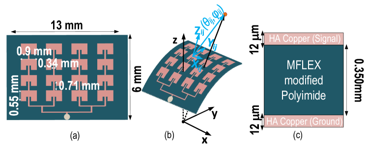
Figure 4: (a) The unfolded rectangular patch antenna array, (b) visual illustration of array bending, (c) metal layer information for the proposed flexible patch antenna array.

For a patch antenna array with m rows and n columns, depicted in Fig. 4(a) (m=n=4), the electric field associated with the arbitrary antenna element located in the i-th row and the j-th column is calculated with respect to its local coordinate system for an observer at ($r_{ij},\theta_{ij},\phi_{ij}$) given by [10]:

$$E^{l}_{\theta_{ij}}=E_{0}(r_{ij})\cos\phi_{ij}\frac{\sin\gamma_{ij}}{\gamma_{ij}}\cos\rho_{ij}$$ (1)

$$E^{l}_{\phi_{ij}}=-E_{0}(r_{ij})\cos\theta_{ij}\sin\phi_{ij}\frac{\sin\gamma_{ij}}{\gamma_{ij}}\cos\rho_{ij}$$ (2)

where

$$\gamma_{ij}=\beta\frac{W}{2}\sin\theta_{ij}\sin\phi_{ij}$$ (3)

$$\rho_{ij}=\beta\frac{L}{2}\sin\theta_{ij}\cos\phi_{ij},$$ (4)

and $W$, $L$, $E_{0}(r)$, are the width and length of each patch antenna and strength of electric field associated with incident power at distance $r$ from the antenna. The exponent $l$ indicates the calculation of the field vectors with respect to the local coordinate system. Moreover, $\theta_{ij}$ and $\phi_{ij}$ are the angles from patch element at $ij$-th location to the target point in the $\theta$ plane and $\phi$ plane, respectively. It is noteworthy that $\gamma_{ij}$ and $\rho_{ij}$ are auxiliary variables defined for the brevity and conciseness of derivations and have no physical significance.

The magnetic fields will be similar to (1) and (2) just with a scaling factor of $\eta$ which is the intrinsic air impedance [11].

The 3-D folding of the antenna array will cause variations in the exact positions and orientations of the array elements. These variations will alter each radiation element’s contribution to the array beam, and subsequently the radiation properties. To capture the arbitrary rotations, a change of coordinate system from spherical to cartesian, allows us to calculate basic rotation matrices $R_{x,ij}$, $R_{y,ij}$ and $R_{z,ij}$. Also, the total $E$ and $H$ vecotr fields in the Cartesian coordinate system can be written as

$$\vec{E}_{ij}(\theta_{ij},\phi_{ij})=\vec{E}_{x_{ij}}(\theta_{ij},\phi_{ij})+\vec{E}_{y_{ij}}(\theta_{ij},\phi_{ij})+\vec{E}_{z_{ij}}(\theta_{ij},\phi_{ij})$$ (5)

where $x_{ij}$,$y_{ij}$, and $z_{ij}$ are the Cartesian coordinates of the target located in the spherical coordinate of ($r_{ij}$, $\theta_{ij}$, $\phi_{ij}$).

For the $m\times n$ antenna array, the angles $\alpha_{x,ij}$, $\alpha_{y,ij}$, and $\alpha_{z,ij}$ represent the corresponding rotation of Cartesian unit vectors at the local coordinate systems when transitioning from the unfolded state to folded state.

The corresponding total rotation of the ij-th antenna element is represented by matrix $R_{tot,ij}$ that is calculated by the matrix product of basic rotation matrices $R_{\alpha_{x,ij}}$, $R_{\alpha_{y,ij}}$, and $R_{\alpha_{z,ij}}$. To transform each local coordinate system into the global coordinate, $R_{tot}^{-1}$ for the $ij$-th element is calculated as follows,

$$R_{tot,ij}^{-1}=\\ \\ \begin{bmatrix}c_{x}^{ij}c_{z}^{ij}-s_{x}^{ij}s_{y}^{ij}s_{z}^{ij}&-s_{x}^{ij}c_{y}^{ij}&c_{x}^{ij}s_{z}^{ij}+s_{x}^{ij}s_{y}^{ij}c_{z}^{ij}\\ s^{ij}_{x}c^{ij}_{z}+c^{ij}_{x}s^{ij}_{y}s^{ij}_{z}&c^{ij}_{x}c^{ij}_{y}&s^{ij}_{x}s^{ij}_{z}-c^{ij}_{x}s^{ij}_{y}c^{ij}_{z}\\ -c^{ij}_{y}s^{ij}_{z}&s^{ij}_{y}&c^{ij}_{y}c^{ij}_{z}\end{bmatrix}$$ (6)

where $s_{w}^{ij}=\sin\alpha_{w,ij}$ and $c_{w}^{ij}=\cos\alpha_{w,ij}$ for $w\in\{x,y,z\}$. For example, $s_{x}^{ij}=\sin\alpha_{x,ij}$ and $c_{y}^{ij}=\cos\alpha_{y,ij}$. In the next step, $E_{ij}(\theta_{ij},\phi_{ij})$ in the global coordinate system should be calculated by applying the $R^{-1}_{tot}$ on the Cartesian unit vectors of electric fields ($E^{x^{l}}_{ij}$,$E^{y^{l}}_{ij}$,$E^{z^{l}}_{ij}$) cascaded with the change of basis (from spherical to cartesian) matrix $T_{CB}$, i.e.,

$$\vec{E}_{ij}(\theta_{ij},\phi_{ij})=R^{-1}_{tot}T_{CB}[0,E_{\theta},E_{\phi}]^{T}$$ (7)

The electric field distribution and amplitude characteristics of an $m\times n$ patch antenna array at a given distance from the center point of the array ($r$) will be calculated as [12]:

$$\vec{E}_{tot}(\theta_{ij},\phi_{ij}) =E_{0}\sum_{i=1}^{m}\sum_{j=1}^{n}\frac{I_{ij}\sin\gamma_{ij}}{\gamma_{ij}}\cos\rho_{ij}\times$$ (8)

$$\quad\left[(\mu_{1})\hat{x}+(\mu_{2})\hat{y}+(\mu_{3})\hat{z}\right]$$

$$|E|(x_{mn},y_{mn},z_{mn}) =E_{0}\sum_{m=1}^{M}\sum_{n=1}^{N}\frac{I_{mn}\sin\gamma_{mn}}{\gamma_{mn}}\cos\rho_{mn}$$ (9)

$$\quad\times\sqrt{(\mu_{1})^{2}+(\mu_{2})^{2}+(\mu_{3})^{2}}$$

Where $\vec{E}_{tot}$ is the summation of the electric fields from all individual antennas calculated based on (7), and $I_{ij}$ is the excitation current of ij-th antenna and:
$\mu_{1}=2\cos\theta_{ij}(c_{x}^{ij}c_{z}^{ij}-s_{x}^{ij}s_{y}^{ij}s_{z}^{ij}),+\cos\phi_{ij}\sin\theta_{ij}c_{y}^{ij}s_{z}^{ij},$
$\mu_{2}=-2\cos\theta_{ij}s_{x}^{ij}c_{y}^{ij}-\cos\phi_{ij}\sin\theta_{ij}s_{y}^{ij}$,
$\mu_{3}=2\cos\theta_{ij}(c_{x}^{ij}s_{z}^{ij}+s_{x}^{ij}s_{y}^{ij}c_{z}^{ij})-\cos\phi_{ij}\sin\theta_{ij}c_{y}^{ij}c_{z}^{ij}.$

The above coefficients capture the effect of bending on the array’s total electric field and by setting $\alpha_{x,ij}=\alpha_{y,ij}=\alpha_{z,ij}=0$, the equations of the unfolded antenna array will be obtained. The total radiated power of the antenna array based on $\vec{E}\times\vec{H}$ is calculated by approximating $\sin\gamma_{ij}\simeq\gamma_{ij}$ and $\cos\rho_{ij}\simeq 1$ as [13]:

$$P_{tot} =\frac{E_{0}^{2}}{2\eta}\int\sum_{i=1}^{m}\sum_{j=1}^{n}\frac{I_{ij}^{2}\sin\gamma_{ij}^{2}}{\gamma_{ij}^{2}}\cos\rho_{ij}^{2}((\kappa_{1})^{2}+(\kappa_{2})^{2})ds$$ (10)

Where $ds=r^{2}\sin\theta d\theta d\phi$, $\kappa_{1}$ and $\kappa_{2}$ are:

$$\kappa_{1} =\cos\theta_{ij}\cos\phi_{ij}\mu_{1}+\cos\theta_{ij}\sin\phi_{ij}\mu_{2}-\sin\theta_{ij}\mu_{3}$$ (11)

$$\kappa_{2} =-\sin\phi_{ij}\mu_{1}+\cos\phi_{ij}\mu_{2}$$

$$P_{tot}=\frac{\sum_{i=1}^{m}\sum_{j=1}^{n}{\pi^{2}E_{0}^{2}I_{ij}^{2}\chi}}{60\eta}$$ (12)

All the parameters that incorporate the effect of folding are represented by $\chi$ parameters which is

$$\chi =64\chi_{1}^{2}+24\chi_{2}+64\chi_{3}+16\chi_{4}+32\chi_{5}^{2}$$ (13)

$$+16\chi_{1}c_{y}^{ij}c_{z}^{ij}+16\chi_{5}c_{y}^{ij}s_{z}^{ij}$$

where$\chi_{1}=c_{x}^{ij}c_{z}^{ij}-s_{x}^{ij}s_{y}^{ij}s_{z}^{ij}$, $\chi_{2}={c_{y}^{ij}}^{2}{s_{z}^{ij}}^{2}$, $\chi_{3}={s_{x}^{ij}}^{2}{c_{y}^{ij}}^{2}$, $\chi_{4}={s_{y}^{ij}}^{2}$, and $\chi_{5}=c_{x}^{ij}s_{z}^{ij}+s_{x}^{ij}s_{y}^{ij}c_{z}^{ij}$. The antenna radiation impedance, $R_{rad}$, based on the measured power is estimated in[14] which is adopted here, i.e.,

$$R_{rad}=\frac{{60mnV_{0}^{2}\eta}}{\sum\limits_{i=1}^{m}\sum\limits_{j=1}^{n}I_{ij}^{2}\pi^{2}E_{0}^{2}\chi}$$ (14)

Where $V_{0}$ denotes the voltage at the edge of input port. By measuring the radiation impedance, the input impedance of the antenna, $Z_{ant}$, will be calculated as:

$$Z_{ant}=R_{rad}\frac{P_{in}}{P_{tot}}+jX_{ant},$$ (15)

which is simplified to a real impedance under negligible values of $X_{ant}$, a condition that is confirmed in the next section.

II-B BER of 6G systems using Bent Antenna Arrays

To capture the impact of antenna bending on the received power by the receiver, we deploy the Friis formula and the received power $P_{r}$ will become

$$P_{r}=P_{t_{\text{max}}}\times G_{T,F}G_{R}\times\frac{\lambda}{\left(4\pi d\right)^{2}}\times\frac{16Z_{PA}^{2}Z_{ant}^{2}}{\left(Z_{PA}+Z_{ant}\right)^{4}},$$ (16)

where $P_{t}$, $G_{T,F}$, $G_{r}$, $\lambda$, and $d$ represent the transmitter power, gain of folded transmitter antenna array, unfolded receiver antenna gain, wavelength, and the distance between the transmitter and receiver, respectively. According to the receiver power in (16), for a 6G QAM transceiver, the signal-to-noise ratio on the receiver side is calculated as [15]:

$$SNR_{Rec}=\frac{P_{r}}{P_{r,n_{in}}+P_{n_{out}}}$$ (17)

Where $P_{r}$, $P_{r,n_{in}}$, and $P_{n_{out}}$ represent the power of the received signal, the power of the received transmitter noise, and the power of the output noise respectively. According to [16], the error-vector magnitude of a QAM constellation is approximated by $1/\sqrt{SNR_{Rec}}$ when number of symbol streams ($T$) is much larger than number of modulation symbols $N$, i.e., ($T\gg N$). Subsequently, the bit-error-rate will be approximated as a function of modulation order, and EVM by

$$\footnotesize P_{b}=\frac{2(1-\frac{1}{L})}{{\log_{2}(L)}}\cdot Q\left(\sqrt{\frac{{3\log_{2}(L)}}{{L^{2}-1}}\cdot\frac{2}{{\text{EVM}^{2}_{RMS}\log_{2}(M)}}}\right)$$ (18)

Where M and L are mode of modulation and the number of levels in each dimension of the M-ary modulation system.

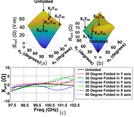
Figure 5: (a) Analytical values versus simulated results for (a) the magnitude of electric field, and (b) input resistance of the 4$\times$4 array, (c) input reactance variations by folding.

III Simulation Results

To assess the analytical derivations in Section II, the $4\times 4$ patch antenna designed based on MFLEX modified polyimide (MPI) material was simulated in Ansys HFSS and four versions with different folding angles on both x- and y-axis were considered. For conciseness, we denote the angle of bending in the x-axis and y-axis by $x_{\xi_{1}},y_{\xi_{2}}$ where $\xi_{1}$ and $\xi_{2}$ are the angle of bending between the first and last antennas in a row or column along the x and y directions, respectively. Other than the unfolded scenario, $x_{9},y_{45}$, $x_{9},y_{90}$, $x_{45},y_{45}$, and $x_{15},y_{45}$ are the simulated versions of the folded antenna array. As shown in Fig. 5(a), the magnitude of radiated electric field changes with the folding angle and for excessively large angles (e.g., $\geq 90^{0}$), the destructive summation of fields from antennas results in weakened radiation intensity. The input impedance of the antenna array, $R_{ant}$, also changes by the folding degree and increases gradually by the bending angle, Fig. 5(b). The simulated electric field and input resistance for the 5 scenarios are shown in ordered pairs comprising magnitude of total electric field and antenna array input impedance, i.e., ($|\vec{E}_{tot}|$,$R_{ant}$), and the values are (51,50), (46,67), (38,62), (30,67), and (46,72) for unfolded, $x_{9},y_{45}$, $x_{9},y_{90}$, $x_{45},y_{45}$, and $x_{15},y_{45}$, respectively. The simulation results match with these analytical equations. Moreover, $X_{ant}$, the reactive part of input impedance, is simulated for various bending scenarios in the x and y directions where the variations are negligible and bounded between $\pm$ 5$\Omega$, Fig. 5(c).

To exploit the beam-steering advantage of the flexible antenna array, three curvature scenarios of concave, flat, and convex both in x any y direction are simulated in HFSS and compared in Fig. 6. It is evident that by folding the array along the y and x axis, the main radiated beam can be tilted corresponding to the folding amount, e.g., from $\theta=-25^{0}$ to $\theta=30^{0}$ in Fig. 6 with little peak gain variation when the curvature changes from concave to convex. To account for the possible beam squint [17] associated with the folding, in Fig.7, the beam stability across the bandwidth is simulated in HFSS where a relatively small squint is observed for both E-plane and H-plane beam rotations. This property serves to utilize this design in 6G systems without a beam squint.

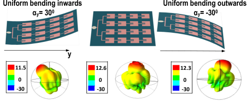
Figure 6: folded Patch array antenna front and side view with radiation pattern

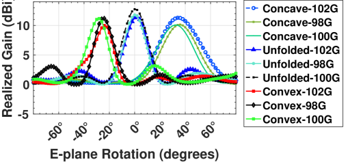
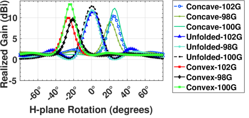
Figure 7: Flexible antenna array beam profile across the bandwidth in (top) E-plane and (bottom) H-plane.

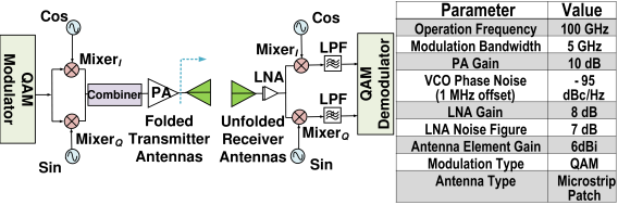
Figure 8: The system level architecture of the simulated 6G wireless system and the design parameters

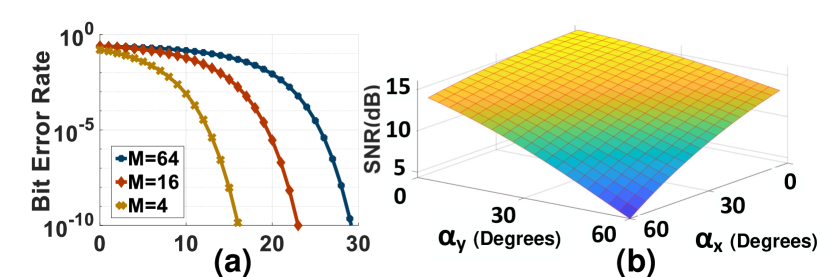
Figure 9: (a) Bit error rate (BER) based on SNR for different modes of QAM, and (b) SNR variation with various folding degrees along the x- and y- axis.

The folded transmitter antenna array was simulated inside a post-layout CMOS-based 6G wireless transceiver shown in Fig. 8 with the listed design parameters. In these simulations, the antenna on the transmitter side is folded and the receiver side is assumed unfolded. Within this configuration, digital baseband QAM signals were generated in the digital signal processor (DSP) and subsequently channeled to two digital-to-analog converters (DACs) for conversion into analog signals. The baseband in-phase (I) and quadrature (Q) components underwent upconversion to Radio Frequency (RF) with the aid of I and Q mixers which have 0 dB conversion gain, driven by quadrature Local Oscillator (LO) signals. The power combination of the two upconverted I and Q components resulted in the generation of the QAM RF signal, poised for transmission to the power amplifier. The amplified signal by the power amplifier that was modulated by the upconverted base-band data, was fed into the folded transmitter antenna array. On the receiver side, the signal was received using the unfolded version of the antenna array and subsequently, was amplified with a low noise amplifier (LNA) and downconvrted by an I-Q mixer. Subsequently, two 4th-order low pass filters (LPF) were utilized to generate the output baseband signal where a digital QAM demodulator was used to extract the output bits. As shown in Fig. 9(a) by increasing the spectral efficiency of QAM modulation, the necessary signal-to-noise ratio to maintain the BER increases [16]. Meanwhile, by excessively folding the transmitter antenna in the 6G wireless system, the SNR decreases. Both simulated BER and analytical values in Table I, suggest that the folded antenna array is a viable choice for 4-QAM and 16-QAM modulations. For 64-QAM modulation, the transmitter maintains a BER within $O(10^{-2})$ for small folding angles. The simulated BER and analytical expressions exhibit a close match.

TABLE I: Simulated and analytical BER for various modes of QAM modulation

Reference	[8]	[18]	[19]	[7]	[20]	This work
Frequency	85 GHz	86 GHz	64 GHz	145 GHz	160 GHz	100 GHz
Type	Active PS*	VM**	Passive PS	Passive PS	Active PS	Flexible Antenna
Insertion loss	7.2 dB	4.99 dB	16.3 dB	11.5 dB	4.5 dB	2 dB
Power (mW)	150 (with PA)	0	0	0	50	0

• PS = phase shifter and **VM = vector modulator

TABLE II: Comparison of Different Beam Rotation Techniques for 6G Communication

IV Conclusion

This work examined the 2-D curvature effects of flexible antenna arrays on the radiation properties as well as communication performance in a 6G wireless system. In addition to proposing experimentally validated package solutions, by evaluating a 97.5-102.5 GHz 4$\times$4 flexible patch antenna array, a beam rotation without peak gain degradation is confirmed up to 60 degrees, without a noticeable beam squint. Moreover, the deployment of the folded antenna array in a CMOS-based QAM transceiver is studied to confirm low BER across the desired bending degrees of the antenna array. As compared against phase shifting techniques in TABLE II, by designing MIMO phased arrays deploying these flexible antennas, the beam alignment can be extended in 2 dimensions beyond the reach of phase shifters while reducing the insertion loss.

References

- [1] Xuyang Liu, Md Hedayatullah Maktoomi, Mahdi Alesheikh, Payam Heydari, and Hamidreza Aghasi, “A 49-63 ghz phase-locked fmcw radar transceiver for high resolution applications,” in ESSCIRC 2023-IEEE 49th European Solid State Circuits Conference (ESSCIRC). IEEE, 2023, pp. 509–512.
- [2] Xiang Yi, Cheng Wang, Xibi Chen, Jinchen Wang, Jesús Grajal, and Ruonan Han, “A 220-to-320-ghz fmcw radar in 65-nm cmos using a frequency-comb architecture,” IEEE Journal of Solid-State Circuits, vol. 56, no. 2, pp. 327–339, 2020.
- [3] Shiji Pan, Francis Caster, Payam Heydari, and Filippo Capolino, “A 94-ghz extremely thin metasurface-based bicmos on-chip antenna,” IEEE Transactions on Antennas and Propagation, vol. 62, no. 9, pp. 4439–4451, 2014.
- [4] Md Hedayatullah Maktoomi, Zisong Wang, Huan Wang, Soheil Saadat, Payam Heydari, and Hamidreza Aghasi, “A sub-terahertz wideband stacked-patch antenna on a flexible printed circuit for 6g applications,” IEEE Transactions on Antennas and Propagation, vol. 70, no. 11, pp. 10047–10061, 2022.
- [5] Mahdi Alesheikh, Rouhollah Feghhi, Fatemeh Modares Sabzevari, Adil Karimov, Masum Hossain, and Karumudi Rambabu, “Design of a high-power gaussian pulse transmitter for sensing and imaging of buried objects,” IEEE Sensors Journal, vol. 22, no. 1, pp. 279–287, 2022.
- [6] Md Hedayatullah Maktoomi, Soheil Saadat, Omeed Momeni, Payam Heydari, and Hamidreza Aghasi, “Broadband antenna design for terahertz communication systems,” IEEE Access, vol. 11, pp. 20897–20911, 2023.
- [7] Mohammadreza Abbasi and Wooram Lee, “A low-loss passive -band phase shifter for calibration-free, precise phase control,” IEEE Journal of Solid-State Circuits, 2024.
- [8] Chun Wang, Pin-Chun Chiu, and Chun-Hsing Li, “A w-band phase-shifter-embedded pa in 40-nm cmos for 6g applications,” in 2023 IEEE/MTT-S International Microwave Symposium - IMS 2023, 2023, pp. 1140–1143.
- [9] Irfan Ahmed, Hedi Khammari, Adnan Shahid, Ahmed Musa, Kwang Soon Kim, Eli De Poorter, and Ingrid Moerman, “A survey on hybrid beamforming techniques in 5g: Architecture and system model perspectives,” IEEE Communications Surveys & Tutorials, vol. 20, no. 4, pp. 3060–3097, 2018.
- [10] Warren L Stutzman and Gary A Thiele, Antenna theory and design, John Wiley & Sons, 2012.
- [11] Constantine A Balanis, Antenna theory: analysis and design, John wiley & sons, 2016.
- [12] Kaiqi Cao, Cheng Jin, Binchao Zhang, Qihao Lv, and Fan Lu, “Beam stabilization of deformed conformal array antenna based on physical-method-driven deep learning,” IEEE Transactions on Antennas and Propagation, vol. 71, no. 5, pp. 4115–4127, 2023.
- [13] James R James and Peter S Hall, Handbook of microstrip antennas, vol. 1, IET, 1989.
- [14] Irfan Ali Tunio, Study of Impedance Matching in Antenna Arrays, Theses, UNIVERSITE DE NANTES, Dec. 2020.
- [15] Behzad Razavi and Razavi Behzad, RF microelectronics, vol. 2, Prentice hall New York, 2012.
- [16] Rishad Ahmed Shafik, Md. Shahriar Rahman, and AHM Razibul Islam, “On the extended relationships among evm, ber and snr as performance metrics,” in 2006 International Conference on Electrical and Computer Engineering, 2006, pp. 408–411.
- [17] Zhijun Liu, Waheed ur Rehman, Xiaodong Xu, and Xiaofeng Tao, “Minimize beam squint solutions for 60ghz millimeter-wave communication system,” in 2013 IEEE 78th Vehicular Technology Conference (VTC Fall). IEEE, 2013, pp. 1–5.
- [18] Mohammad Montaseri, Mostafa Jafari-Nokandi, Aarno Pärssinen, and Timo Rahkonen, “Analysis of hbt vector modulator phase shifters based on gilbert cell for sub-thz regimes,” in 2020 IEEE International Symposium on Circuits and Systems (ISCAS), 2020, pp. 1–5.
- [19] Fanyi Meng, K. MA, Kiat Seng Yeo, and Shanshan xu, “A 57-to-64-ghz 0.094-mm² 5-bit passive phase shifter in 65-nm cmos,” IEEE Transactions on Very Large Scale Integration (VLSI) Systems, vol. 24, pp. 1–1, 09 2015.
- [20] David del Rio, Iñaki Gurutzeaga, Roc Berenguer, Ismo Huhtinen, and Juan Francisco Sevillano, “A compact and high-linearity 140–160 ghz active phase shifter in 55 nm bicmos,” IEEE Microwave and Wireless Components Letters, vol. 31, no. 2, pp. 157–160, 2021.