Bias Begets Bias: the Impact of Biased Embeddings on Diffusion Models
Abstract
With the growing adoption of Text-to-Image (TTI) systems, the social biases of these models have come under increased scrutiny. Herein we conduct a systematic investigation of one such source of bias for diffusion models: embedding spaces. First, because traditional classifier-based fairness definitions require true labels not present in generative modeling, we propose statistical group fairness criteria based on a model’s internal representation of the world. Using these definitions, we demonstrate theoretically and empirically that an unbiased text embedding space for input prompts is a necessary condition for representationally balanced diffusion models, meaning the distribution of generated images satisfy diversity requirements with respect to protected attributes. Next, we investigate the impact of biased embeddings on evaluating the alignment between generated images and prompts, a process which is commonly used to assess diffusion models. We find that biased multimodal embeddings like CLIP can result in lower alignment scores for representationally balanced TTI models, thus rewarding unfair behavior. Finally, we develop a theoretical framework through which biases in alignment evaluation can be studied and propose bias mitigation methods. By specifically adapting the perspective of embedding spaces, we establish new fairness conditions for diffusion model development and evaluation.
1 Introduction
As Text-To-Image (TTI) models become increasingly adept at generating complex and realistic images, they are being integrated into a wide range of commercial and creative services (Ramesh et al., 2021; Rombach et al., 2022; Saharia et al., 2022). The proliferation of these models is evident in various industries; for example, advertising agencies use them to quickly generate visual content for campaigns, while film and game developers employ them to design detailed backgrounds and characters. The ubiquity of these models, however, has also raised significant ethical and fairness concerns, from their potential for misuse to the biases they encode. Addressing these issues is critical to developing TTI models that are not only technologically advanced but also socially responsible and inclusive.
Here, we specifically study diffusion models, a class of models that form the centerpiece of most advanced TTI systems. We first consider direct representational harm; that is, breaches of fairness that arise from generations that are imbalanced across different protected classes. In the literature, it is generally “well-established” that most diffusion models have imbalanced representation in their generations. For instance, Perera & Patel (2023) show that popular TTI models consistently underrepresent minorities in most professions, a finding corroborated by several other papers (Wang et al., 2023; Luccioni et al., 2023; Wan et al., 2024).
Violations of fairness also arise indirectly; most prominently, a model that generates lower quality images of one group versus another creates indirect representational harm. To audit this type of harm, one important evaluation criteria on which TTI models are often benchmarked is the alignment/faithfulness of images to prompts—how well the contents of the generated image match the prompt. If generated images are well-aligned with the prompt across classes, then the model treats these groups equally. While some papers attempt to use human ratings for benchmarking (Lee et al., 2023), this approach is expensive and hard to scale; thus, more recent work has explored automating alignment evaluation. One method growing in popularity is CLIPScore, based on the text-image embedding CLIP (Radford et al., 2021), which measures the cosine similarity between a prompt and an image in the multimodal latent space (Hessel et al., 2022).
Embeddings play a critical role in generating from and evaluating diffusion models. Besides the dataset a model is trained on, the text embedding of the prompt is the only input to a diffusion model; similarly, many popular approaches for prompt-image alignment leverage a joint text-image latent space. Despite their critical role, however, few papers focus on connecting properties of embedding spaces to downstream fairness criteria. In this paper, we demonstrate that two intuitive conclusions hold both theoretically and empirically. In Section 4, we show that biased embeddings cause biased generations in diffusion models. In Section 5, we show biased image-text embedding spaces lead to biased evaluation of prompt-image alignment for any TTI model. As modern machine learning systems increasingly integrate many components, like learned embeddings, our work highlights that the fairness of each part is critical for ensuring the fairness of the whole.
2 Related Work
Theory of Algorithmic Fairness. Existing work in algorithm fairness has concentrated on the setting of supervised learning, where individuals are mapped to outcomes. Traditionally, group fairness notions (like statistical parity) enforce some measure of average equal treatment between members of protected classes, whereas individual fairness notions require similar individuals to be treated similarly, under some task-specific metric (Dwork et al., 2011). More recently, multi-group fairness has emerged as a middle ground, which enforces fairness constraints on (up to exponentially many) subgroups within the dataset. One such notion is multicalibration (Hebert-Johnson et al., 2018), on which we base our work in Section 5, although others have also been proposed (Kearns et al., 2018).
Theory of Diffusion Models. In brief, diffusion models sample from some distribution of images by learning how much noise gets added to images over time so images can be sampled from that distribution by denoising a sample of pure Gaussian noise; the denoising function at time is the same as the statistical score of the noised distribution (Song et al., 2020). Mathematically, the convergence to the true distribution of the sampling process with a sufficiently good approximation of the score can be proved with Girsanov’s thoerem (Theorem A.2); empirically, the process is implemented via a discrete-time approximation, where we iteratively denoise images over small time steps. We defer a full theoretical coverage of diffusion models to Appendix A, and note that we later leverage Theorem A.2 for our proof that biased embeddings cause biased generations.
Bias in Embedding Spaces. Bolukbasi et al. (2016) was the first to demonstrate bias present in word embeddings on the basis of gender, and proposed methods to debias such embeddings, followed by similar work on bias in race (Manzini et al., 2019; Dev & Phillips, 2019). Papakyriakopoulos et al. (2020) train a sentiment classifier on a biased word embedding and illustrate that the downstream classifier’s outputs reflect the direction of biases in the input embedding. These biases have also been observed in multimodal embeddings like CLIP (Wang et al., 2021; Berg et al., 2022), and the impact of these biases on evaluating image captioning methods has been studied (Qiu et al., 2023). However, to our knowledge, our work is the first to analyze the effect of bias in learned embedding spaces like CLIP on the evaluation of TTI systems, as well as the downstream impact of a biased embedding as a component of a generative model.
Bias in Diffusion Models. Several recent papers on fairness in diffusion models propose methods to sample with more equal representation across protected classes (Li et al., 2024; Friedrich et al., 2023; Choi et al., 2024; Shen et al., 2024; Chuang et al., 2023). Of note, Chuang et al. (2023) and Li et al. (2024) intervene on the prompt embedding, using a debiasing projection and a learned fair representation of prompts, respectively. Both works illustrate that debiasing embeddings leads to more representationally fair generations. In Section 4, we show this is a necessary condition.
Prompt-Image Alignment. There are several papers that attempt to benchmark the prompt-image alignment of image generation models. Of these, Lee et al. (2023) rely most heavily on CLIPScore for alignment evaluation. Bakr et al. (2023) use CLIPScore for more specific evaluation criteria like generation of emotion. Chen et al. (2024) define a composite metric called ‘text condition evaluation’ that encompasses alignment and fairness. To calculate the alignment portion of their score, the authors utilize a visual question answering (VQA) model called BLIP (Li et al., 2022). Bakr et al. (2023) and Chen et al. (2024) also raise concerns with utilizing CLIPScore to measure alignment, but do not cite fairness as a concern. There have been several other attempts at evaluating text-image alignment (Hu et al., 2023; Xu et al., 2023; Yarom et al., 2023), all of which potentially demonstrate some form of implicit bias due to their reliance on external models. In this paper, we introduce a framework for studying these biases irrespective of the underlying alignment score function used.
Algorithmic Fairness for Generative Models. In the traditional theory of algorithmic fairness for supervised classifiers, individuals self-identify into different categories and fair algorithms provide guarantees with respect to how individuals in different (sub)groups are treated (Feldman et al., 2015). With generative models, however, we run up against a fundamental epistemic question of identification: generations have no underlying classifications. While most extant literature on fairness in TTI models relies on a different classifier to categorize generations (Friedrich et al., 2023; Shen et al., 2024), this method suffers from two core flaws. First, it relies on physical features alone to define categories, which has the potential to reify stereotypes. Second, these classifiers still exhibit various social biases reflected in their training data (Luccioni et al., 2023); in fact, Section 5 demonstrates that the biases of such classifiers impairs model evaluation. To this end, we attempt to leverage the model’s internal representation of the world in order to construct notions of fairness when defining biased generations. In particular, we imagine that the model knows the class from which it is generating; while we don’t have access to this latent truth, we can operationalize our definitions around it, as we do in Section 4.
3 Preliminaries
Here, we introduce some notation that we will use throughout the manuscript. Let denote the total variation distance. Let denote the set of all prompts (e.g. ‘an image of a doctor interacting with a patient’) and to denote the set of all images. A text-to-image model takes a prompt as the input and returns a distribution over images that can be sampled from. A multimodal embedding consists of a pair of functions , where . We use the set to refer to possible attributes such as race or gender specifiers (e.g. ‘female’) and to denote the base prompt (e.g. ‘firefighter,’ or more generally any descriptor independent of ). For some , the operation represents the prompt obtained by combining an attribute and a base prompt. For example, for and , we have . We also use to denote the map from prompts to prompt embeddings within a diffusion model. Let be the distribution over images generated by the model conditioned on text prompt . The above notation applies to any text-to-image model; for diffusion models specifically, let denote the learned score function of input and time conditioned on a prompt embedding . Let be the length of the denoising period.
4 Biased Embedding, Biased Generations
In Theorem 4.5, we prove that sufficiently strong bias in the prompt embeddings implies representational imbalance in the image generations. We start with some intuition to interpret the result. Suppose we have a base prompt and attributes and . If the embedding of is sufficiently close to the embedding for and images with the attributes and are distinguished from each other, Theorem 4.5 states that the diffusion model conditioned on will mostly produce images similar to when it is conditioned on . Thus most of the images generated from ‘nurse’ would be of ‘woman nurse’, which is exactly representational bias in sampling. To formalize this, we first operationalize our notions of biased prompt embeddings and representational balance that will be relevant throughout this section.
Biased Embeddings. Extant literature on biased embeddings identifies imbalanced distances between words (e.g. if ‘woman’ is closer to ‘nurse’ than ‘man’). We leverage a similar, albeit more general, notion here.
Definition 4.1.
Given set of attributes , base prompt , and some , an embedding for is -close to if .
This is extremely similar to the definition of bias from Bolukbasi et al. (2016), which computes the projection of some base prompt to a learned gender direction. Directly computing the distance between a base prompt and the base prompt with an associated attribute is a natural extension of this idea and also circumvents the assumption in Bolukbasi et al. (2016) that there is an explicit gender direction in the latent space. While closeness does not immediately imply a problematic embedding (e.g. if is large), common biases in embeddings satisfy -closeness to some with small (i.e. places the base prompt closer to some protected attribute than others).
Representational Balance. Now that we have defined a biased embedding, we define our definition of fairness. Informally, a model is representationally balanced if the proportion of images generated of prompt with attribute is at least for . In this section, we rely on the model’s own representations for different attributes .
Definition 4.2.
A model is representationally balanced with respect to attribute set , base prompt , and constants if and for .
This both ensures that produces at least -proportion of images in the support of and that does not place too much mass on images that are unlikely to be generated by . To gain intuition into this definition, we can view as a mixture model consisting of images with and without , with mixture weights and , respectively. If the components are disjoint and equals the component of images with , then we have exactly . We note that this definition does not control for small discrepancies between sampling directly from versus sampling from and conditioning on belonging to the support of . For example, let place mass on three images, and places mass of on the same images. Clearly the is still , and this is representationally fair for , but the -images generated by are different than those generated by . This example arises because our Definition 4.2 is a group fairness notion. For finer control over representation of specific images, one can concatenate subsets of attributes together for multi-group representational control; we view this line of work as an interesting future direction.
We now state the two assumptions of Theorem 4.5. The most important one is that the score function is Lipschitz with respect to the prompt embeddings (Assumption 4.3). Lipschitzness of the learned score function in the first argument is standard in the theory of diffusion literature, e.g., Chen et al. (2023). This assumption can also be interpreted as an individual fairness constraint, where the requirement that similar prompt embeddings produces similar images parallels the notion that similar individuals are mapped to similar outcomes (Dwork et al., 2011). Assumption 4.4 codifies the requirement that represent distinct categories, which is necessary to show violations of our definition of representational balance because it implies that over-representation of one group limits representation of other groups.
Assumption 4.3 (Lipschitz in prompt embeddings).
The score of the diffusion model is -Lipschitz in .
Assumption 4.4 (Distinct categories of identifiers).
There exists such that for all distinct , .
Now we formally state Theorem 4.5.
Theorem 4.5 (Bias in embeddings implies bias in image generations).
Proof.
We first show that . We will do this by writing a bound on , and translating it to a bound on total variation via Pinsker’s Inequality. First, we leverage Theorem A.2, which bounds the KL divergence by the quantity
To evaluate this, we note that by Assumption 4.3, we have an upper bound for all . Hence,
Finally, applying Pinsker’s Inequality, we have that
where the last inequality comes via our -close assumption.
Next, we exhibit for . By the reverse triangle inequality,
By Assumption 4.4, we have that for , so in total we have that
∎
This theorem implies that a base prompt sufficiently close to in the embedding will have total variation bounded by between the resulting distributions; similarly, because the attributes are distinct, the total variation between and for is lower-bounded by . Hence, is generated more, breaking representational balance. Note that an -close prompting embedding is an extremely strong requirement yet necessary to meaningfully control the total variation. As such, we next turn to an empirical investigation of the relationship between bias in prompt embeddings and representational imbalance to verify our theoretical conclusions.
Empirics. Previous work has illustrated that the output of diffusion models is not representationally balanced. For instance, Friedrich et al. (2023) illustrate gender bias in the outputs of occupations queried of Stable Diffusion which reflect both the direction of biases in CLIP embeddings and representational imbalances in the underlying training dataset. We find a similar relationship when comparing generations across occupations from Stable Diffusion 2.1 (SD2.1) against biases in the underlying CLIP embedding.
Since SD2.1 is trained on an underlying dataset (LAION-5B) that is itself representationally imbalanced, however, it is unclear if the bias in image outputs is caused by a biased prompt embedding or imbalanced training dataset. To probe this, we train a conditional diffusion model from scratch with balanced training data across three classes (nurse, philosopher, and person) but with biased prompt embeddings (where nurse is closer to woman, philosopher is closer to man, and person is roughly equidistant). We find that the resulting model is biased in its generations in the same direction as the embedding, with women as the majority of nurse generations, men as the majority of philosopher generations, and a roughly even split in generations of people. We defer the full experimental details to Appendix B.2.
5 Bias in Alignment Auditing
In this section we consider the problem of auditing image generation models for prompt-image alignment and analyze the impact that biased multimodal embeddings may have on the fairness of alignment scores. We note that from here on out, we refer to “score” as the alignment score, not the learned function of a diffusion model. While the results in Section 4 studies the representational harm in the generations of biased diffusion models, this section analyzes harms caused by biased alignment predictors and therefore borrows from richer notions of fairness proposed for classification systems. We define a notion of fairness for alignment functions and demonstrate necessary conditions for multimodal embeddings to satisfy this definition. Additionally, we evaluate the bias of existing auditing functions and suggest simple techniques for mitigating such biases.
5.1 Definitions of Fairness
We begin by defining what it means for an alignment auditing function to be fair. These definitions are inspired by existing work on fairness for predictors introduced by (Hebert-Johnson et al., 2018), and are designed to capture the idea that the alignment of an image with a prompt should be independent of protected attributes like race and gender when they are not explicitly specified in the prompt. Note that this differs from our definition of representational balance in Section 4: the auditing function outputs a scalar, allowing us to borrow definitions from the rich extant fairness literature. We use to denote the true alignment score and to denote an auditing function.
Definition 5.1 (Multiaccuracy).
Let be a collection of subsets of and . An auditing function is -multiaccurate for prompt if, for all ,
In other words, multiaccuracy for a prompt ensures that the function is -accurate on every subset of images . To see how this notion is useful for fairness, consider a set of protected attributes for a base prompt , and let be a subset of images corresponding to prompt with attribute . If , -multiaccuracy guarantees that the auditing function is -accurate on average on each of the protected attributes. Thus, for example, if the prompt we care about is “doctor” and the attributes we care about encompass gender, setting and to images of male and female doctors respectively gives us the guarantee that is -accurate on both genders.111Note that gender is not a binary, and we would hope that generative models are able to capture gender on a spectrum. We use male and female in the example for ease of notation. We analyze the strengths and weaknesses of multiaccuracy and define a stronger fairness guarantee based on multicalibration in Appendix C.1.
To see why these notions of fairness are useful for auditing text-to-image models, we prove the following theorem. Intuitively, this theorem states that if we have subsets of images with particular attributes such that the true alignment is equal in expectation across attributes, and if the auditor is multiaccurate on these subsets of images, then the alignment score remains stable irrespective of how a text-to-image model chooses to sample from these attributes.
Theorem 5.2.
Consider a base prompt and attributes , and let be a subset of images corresponding to prompt with attribute . Assume that for all . Let . Consider a model that, given the prompt , returns an image with probability , where . If the auditing function is -multiaccurate, then irrespective of the probabilities .
Proof.
We see that
By the same logic, we also see that . Thus, , so . ∎
As a corollary of this theorem, we see that irrespective of the probabilities , the difference in the alignment score of two models is at most . Thus, going back to our example of male and female doctors, we see that as long as we expect the average alignment of an image of a male doctor and a female doctor with the prompt “doctor” to be the same, if our auditing function is multiaccurate on the appropriate subsets of images, models will get similar alignment scores irrespective of what proportion of male or female doctors they generate.
Finally, it is worth noting that checking whether an auditing function is multiaccurate may be challenging, since this requires access to the true alignment scores . Note that if we had arbitrary oracle access to there would be no need to evaluate auditing functions at all, since we could just use to audit the alignment of text-to-image models. However, the advantage of our notion of fairness is that it only requires “true” scores for a diverse but fixed set of images on which auditing functions can then be evaluated. Such datasets could be obtained by manual labeling, and there have been several efforts to create large image-caption datasets with alignment ratings (Levinboim et al., 2021; Lee et al., 2021; Vedantam et al., 2015; Hodosh et al., 2013).
5.2 Properties of Fair Embeddings
In this section, we explore necessary conditions for multi-modal embeddings to satisfy multiaccuracy. Let us begin by defining an auditing function in terms of a multi-modal embedding space. For vectors and , we define their cosine similarity as Given a multimodal embedding , we define the auditing function This ensures that . Note that existing techniques like CLIPScore (Hessel et al., 2022) achieve a similar effect by clipping the cosine similarity at a minimum of 0, but this is equivalent to our definition up to a factor of 2 as long as similarity is positive.
Given the definitions of fairness for alignment auditors in Section 5.1, it is natural to ask what properties we would expect from a multimodal embedding space in order to obtain a fair auditor. We start with the following observation, which provides a necessary condition for multiaccuracy based on the average score between a prompt and different subsets of images.
theoremtextimage If is -multiaccurate for a prompt , for all , if , then .
Proof.
Since is -multiaccurate for prompt , for all we know that
Moreover, for some , if , by the triangle inequality we see that
Substituting the definition of , we see that
∎
This implies that given a prompt and subsets of images with similar average true alignment scores, if the embeddings of those images do not have a similar distance (on average) to the embedding of then our auditor is not multiaccurate on those images.
Next, we use this observation to detect bias based only on the prompt embeddings . As discussed in Section 4, prompt embeddings are often biased in themselves, which causes bias in diffusion models when these embeddings are used as inputs. By showing that fair prompt embeddings are necessary for multiaccuracy, the theorem below demonstrates that bias in prompt embeddings also translates to bias in multimodal embeddings, and therefore results in biased alignment auditing.
theoremtexttext Consider a prompt and attributes . Let be a set of images such that for every , is in a ball of radius around . For , if is -multiaccurate for prompt , for any such that , it holds that .
Proof.
Since is -multiaccurate for prompt , if , we know by Section 5.2 that
Next, consider the expression . For all , since is in a ball of radius around , we know that there exists a vector such that and . Thus, we see that
Since , we know that . Thus,
for all , which implies that
By symmetry, note that the same expression holds for and . Thus, by the triangle inequality,
∎
The contrapositive of this theorem implies that, for a prompt , if there are two attributes and such that the embeddings of and are not equidistant from the embedding of , then a multiaccurate auditing function derived from this embedding can not be fair on images that closely match attributes and .
Thus, if the underlying embedding space is not fair on prompts, we should not expect it to be a fair auditor. This allows us to infer bias in a multimodal embedding space by only looking at its prompt embedding function .
5.3 Auditing Alignment with Biased Embeddings
While there have been some efforts to debias CLIP and CLIPScore (Dehdashtian et al., 2024), it is likely that many of the approaches we use to audit prompt-image alignment will continue to exhibit some form of representational bias. Thus, it is important to consider methods to mitigate this bias in the score calculation phase. Currently, the standard method for calculating the alignment score of a model for a prompt using a multimodal embedding is to take the average of the auditing function described in Section 5.2 over several images samples from (Lee et al., 2023). Henceforth, we will refer to this method as score-then-average. As we have discussed, one of the ways in which an embedding space may be biased is if for a prompt , vectors corresponding to images with attribute are more similar to the vector for on average than those with attribute . In this case, a model that generates only images with attribute will consistently get a higher alignment score than a model that generates a balanced distribution of images. In this section, we suggest an alternative method of evaluating alignment based on potentially biased multimodal embeddings that helps alleviate this form of bias. Intuitively, this method measures the maximum similarity score between an image and the base prompt with different protected attributes attached. We call this method subclass-score.
In this approach, given a prompt , we begin with a list of attributes on which we would like to be fair. To calculate the alignment score of a model of this prompt, we start by sampling a set of images from . We then calculate the individual scores of images as
For example, if and , . Finally, to calculate the aggregate score we take the average of over images .
This aims to tackle the issue where embeddings of images with one attribute may be closer on average to the embedding of the prompt than images with other attributes. By measuring the similarity with attribute-specific vectors instead, the relative distance from the embedding of the original prompt is no longer an issue. We note that there remain drawbacks with this approach. First, it may be difficult to identify what attributes are appropriate for which prompts. For instance, Google’s Gemini model recently attempted to impose diversity into prompts where it was not historically accurate or appropriate (Gautam et al., 2024). Also, this does not guarantee fairness conditions like multiaccuracy. For example, it is possible that images with some attribute are closer on average to the prompt than another attribute are to the prompt .
We introduce a second method for generating unbiased alignment scores, average-then-score, in Appendix C.2. This method involves taking the mean of the image embeddings before computing the cosine similarity to the prompt embedding. We evaluate and compare these approaches in Section 5.4.
5.4 Empirical Case-Study: CLIP
In this section, we investigate biases present in an existing method of alignment auditing called CLIPScore (Hessel et al., 2022) based on the multimodal embedding model CLIP (Radford et al., 2021). We then evaluate the techniques proposed in Section 5.3. We find that the text embeddings of CLIP demonstrate gender bias in the representation of occupations, matching the findings of (Bolukbasi et al., 2016). We also find that a similar bias is present in the relationship between text embeddings of occupations and gendered image embeddings. In particular, we see that for the same set of images, male medical professionals got a 0.02 higher score than female medical professionals on average for the prompt “doctor,” and a 0.061 lower score for the prompt “nurse.” This clearly demonstrates an underlying bias in the auditing CLIPScore function; models that generate only male doctors and only female nurses get over higher alignment scores than models with balanced distributions. Finally, we evaluate our bias mitigation methods in Section 5.3 and find that subclass-score performs significantly better than average-then-score, staying roughly consistent across gender ratio. Thus, subclass-score is the a promising step for alleviating gender bias in alignment scores for text-to-image models. Further details can be found in Appendix C.3.3.
6 Conclusion and Future Work
In this paper we study the relationship between bias in embeddings and image generations for text-to-image models. We propose new statistical fairness criteria for generative models, and we prove theoretically and empirically that biased prompt embeddings lead to representationally unfair outputs. This establishes a necessary condition (an unbiased embedding) for an unbiased model. We then investigate the impact of biased prompt embeddings on measuring the alignment between image generations and prompts, as well as multi-accuracy and multi-calibration style definitions for fair alignment auditing algorithms.
There are several interesting directions to take this work. First, the text embedding’s impact on fairness in diffusion models can be further investigated empirically with recently-released open state-of-the-art models that have public training sets (Gokaslan et al., 2023). Next, we are interested in potential augmentations for training or evaluating diffusion models that would compensate for bias in embedding spaces. Finally, while we give several conditions that imply a metric-based auditing function is not fair, it would be interesting to to explore sufficient conditions for fairness, like in (Dwork et al., 2011).
Throughout our manuscript, we have worked around the question of true labels (e.g. race/gender) of artificial generations. In the traditional algorithmic fairness setting of supervised learning, we are satisfied with group algorithmic fairness guarantees because the underlying subjects self-identify into specific groups. Generated images have no such ground truth, which is why we proposed group fairness criteria in Section 4 that bypass these labels. Luccioni et al. (2023) proposes using Visual Question Answering model (VQA) for this purpose, but this introduces another source of bias with the VQA model. We hope that future literature provides a sound resolution to this epistemic question underlying any fairness auditing algorithm for text-to-image models.
Acknowledgements
The authors would like to thank Cynthia Dwork for teaching a class which inspired this project, many thoughtful discussions on fairness in generative models, and her abundant questions/suggestions which have greatly improved the clarity of this manuscript. Additionally, the authors would like to thank the ICML Workshop on Trustworthy Multimodal Foundation Models and Agents (TiFA) for featuring an initial version of this work, and comments from its poster/lightning talk. ML would also like to thank Sitan Chen for introducing him to the theory of diffusion models.
Social Impact Statement
As diffusion models become more broadly used in diverse contexts and applications, it is important that their outputs follow various fairness desiderata. This paper studies several of these desiderata, and provides new methodologies and theoretical frameworks for auditing fairness in diffusion models. We also conduct extensive experiments on real diffusion models. We look forward to future research that will further investigate the questions we raise and consider and provide inclusive solutions.
References
- Bakr et al. (2023) Bakr, E. M., Sun, P., Shen, X., Khan, F. F., Li, L. E., and Elhoseiny, M. Hrs-bench: Holistic, reliable and scalable benchmark for text-to-image models, 2023.
- Berg et al. (2022) Berg, H., Hall, S. M., Bhalgat, Y., Yang, W., Kirk, H. R., Shtedritski, A., and Bain, M. A prompt array keeps the bias away: Debiasing vision-language models with adversarial learning, 2022.
- Bolukbasi et al. (2016) Bolukbasi, T., Chang, K.-W., Zou, J., Saligrama, V., and Kalai, A. Man is to computer programmer as woman is to homemaker? debiasing word embeddings, 2016.
- Chen et al. (2024) Chen, M., Liu, Y., Yi, J., Xu, C., Lai, Q., Wang, H., Ho, T.-Y., and Xu, Q. Evaluating text-to-image generative models: An empirical study on human image synthesis, 2024.
- Chen et al. (2023) Chen, S., Chewi, S., Li, J., Li, Y., Salim, A., and Zhang, A. Sampling is as easy as learning the score: theory for diffusion models with minimal data assumptions. In The Eleventh International Conference on Learning Representations, ICLR 2023, Kigali, Rwanda, May 1-5, 2023. OpenReview.net, 2023. URL https://openreview.net/pdf?id=zyLVMgsZ0U_.
- Choi et al. (2024) Choi, Y., Park, J., Kim, H., Lee, J., and Park, S. Fair sampling in diffusion models through switching mechanism, 2024.
- Chuang et al. (2023) Chuang, C.-Y., Jampani, V., Li, Y., Torralba, A., and Jegelka, S. Debiasing vision-language models via biased prompts, 2023.
- Dehdashtian et al. (2024) Dehdashtian, S., Wang, L., and Boddeti, V. N. Fairerclip: Debiasing clip’s zero-shot predictions using functions in rkhss, 2024.
- Dev & Phillips (2019) Dev, S. and Phillips, J. Attenuating bias in word vectors, 2019.
- Dwork et al. (2011) Dwork, C., Hardt, M., Pitassi, T., Reingold, O., and Zemel, R. Fairness through awareness, 2011.
- Feldman et al. (2015) Feldman, M., Friedler, S. A., Moeller, J., Scheidegger, C., and Venkatasubramanian, S. Certifying and removing disparate impact. In Proceedings of the 21th ACM SIGKDD International Conference on Knowledge Discovery and Data Mining, KDD ’15, pp. 259–268, New York, NY, USA, 2015. Association for Computing Machinery. ISBN 9781450336642. doi: 10.1145/2783258.2783311. URL https://doi.org/10.1145/2783258.2783311.
- Friedrich et al. (2023) Friedrich, F., Brack, M., Struppek, L., Hintersdorf, D., Schramowski, P., Luccioni, S., and Kersting, K. Fair diffusion: Instructing text-to-image generation models on fairness, 2023.
- Gautam et al. (2024) Gautam, S., Venkit, P. N., and Ghosh, S. From melting pots to misrepresentations: Exploring harms in generative ai, 2024.
- Gokaslan et al. (2023) Gokaslan, A., Cooper, A. F., Collins, J., Seguin, L., Jacobson, A., Patel, M., Frankle, J., Stephenson, C., and Kuleshov, V. Commoncanvas: An open diffusion model trained with creative-commons images. arXiv preprint arXiv:2310.16825, 2023.
- Hebert-Johnson et al. (2018) Hebert-Johnson, U., Kim, M., Reingold, O., and Rothblum, G. Multicalibration: Calibration for the (Computationally-identifiable) masses. In Dy, J. and Krause, A. (eds.), Proceedings of the 35th International Conference on Machine Learning, volume 80 of Proceedings of Machine Learning Research, pp. 1939–1948. PMLR, 10–15 Jul 2018. URL https://proceedings.mlr.press/v80/hebert-johnson18a.html.
- Hessel et al. (2022) Hessel, J., Holtzman, A., Forbes, M., Bras, R. L., and Choi, Y. Clipscore: A reference-free evaluation metric for image captioning, 2022.
- Ho et al. (2020) Ho, J., Jain, A., and Abbeel, P. Denoising diffusion probabilistic models. Advances in Neural Information Processing Systems, 33:6840–6851, 2020. URL https://arxiv.org/abs/2006.11239.
- Hodosh et al. (2013) Hodosh, M., Young, P., and Hockenmaier, J. Framing image description as a ranking task: Data, models and evaluation metrics. Journal of Artificial Intelligence Research, 47:853–899, 2013.
- Hu et al. (2023) Hu, Y., Liu, B., Kasai, J., Wang, Y., Ostendorf, M., Krishna, R., and Smith, N. A. Tifa: Accurate and interpretable text-to-image faithfulness evaluation with question answering, 2023.
- Kearns et al. (2018) Kearns, M., Neel, S., Roth, A., and Wu, Z. S. Preventing fairness gerrymandering: Auditing and learning for subgroup fairness. In International conference on machine learning, pp. 2564–2572. PMLR, 2018.
- Lee et al. (2021) Lee, H., Yoon, S., Dernoncourt, F., Bui, T., and Jung, K. UMIC: An unreferenced metric for image captioning via contrastive learning. In Zong, C., Xia, F., Li, W., and Navigli, R. (eds.), Proceedings of the 59th Annual Meeting of the Association for Computational Linguistics and the 11th International Joint Conference on Natural Language Processing (Volume 2: Short Papers), pp. 220–226, Online, August 2021. Association for Computational Linguistics. doi: 10.18653/v1/2021.acl-short.29. URL https://aclanthology.org/2021.acl-short.29.
- Lee et al. (2023) Lee, T., Yasunaga, M., Meng, C., Mai, Y., Park, J. S., Gupta, A., Zhang, Y., Narayanan, D., Teufel, H. B., Bellagente, M., Kang, M., Park, T., Leskovec, J., Zhu, J.-Y., Fei-Fei, L., Wu, J., Ermon, S., and Liang, P. Holistic evaluation of text-to-image models, 2023.
- Levinboim et al. (2021) Levinboim, T., Thapliyal, A. V., Sharma, P., and Soricut, R. Quality estimation for image captions based on large-scale human evaluations. In Toutanova, K., Rumshisky, A., Zettlemoyer, L., Hakkani-Tur, D., Beltagy, I., Bethard, S., Cotterell, R., Chakraborty, T., and Zhou, Y. (eds.), Proceedings of the 2021 Conference of the North American Chapter of the Association for Computational Linguistics: Human Language Technologies, pp. 3157–3166, Online, June 2021. Association for Computational Linguistics. doi: 10.18653/v1/2021.naacl-main.253. URL https://aclanthology.org/2021.naacl-main.253.
- Li et al. (2022) Li, J., Li, D., Xiong, C., and Hoi, S. Blip: Bootstrapping language-image pre-training for unified vision-language understanding and generation, 2022.
- Li et al. (2024) Li, J., Hu, L., Zhang, J., Zheng, T., Zhang, H., and Wang, D. Fair text-to-image diffusion via fair mapping, 2024.
- Luccioni et al. (2023) Luccioni, A. S., Akiki, C., Mitchell, M., and Jernite, Y. Stable bias: Analyzing societal representations in diffusion models, 2023.
- Manzini et al. (2019) Manzini, T., Yao Chong, L., Black, A. W., and Tsvetkov, Y. Black is to criminal as Caucasian is to police: Detecting and removing multiclass bias in word embeddings. In Burstein, J., Doran, C., and Solorio, T. (eds.), Proceedings of the 2019 Conference of the North American Chapter of the Association for Computational Linguistics: Human Language Technologies, Volume 1 (Long and Short Papers), pp. 615–621, Minneapolis, Minnesota, June 2019. Association for Computational Linguistics. doi: 10.18653/v1/N19-1062. URL https://aclanthology.org/N19-1062.
- Nichol & Dhariwal (2021) Nichol, A. and Dhariwal, P. Improved denoising diffusion probabilistic models, 2021.
- Papakyriakopoulos et al. (2020) Papakyriakopoulos, O., Hegelich, S., Serrano, J. C. M., and Marco, F. Bias in word embeddings. In Proceedings of the 2020 conference on fairness, accountability, and transparency, pp. 446–457, 2020.
- Perera & Patel (2023) Perera, M. V. and Patel, V. M. Analyzing bias in diffusion-based face generation models, 2023.
- Qiu et al. (2023) Qiu, H., Dou, Z.-Y., Wang, T., Celikyilmaz, A., and Peng, N. Gender biases in automatic evaluation metrics for image captioning, 2023. URL https://arxiv.org/abs/2305.14711.
- Radford et al. (2021) Radford, A., Kim, J. W., Hallacy, C., Ramesh, A., Goh, G., Agarwal, S., Sastry, G., Askell, A., Mishkin, P., Clark, J., Krueger, G., and Sutskever, I. Learning transferable visual models from natural language supervision, 2021.
- Ramesh et al. (2021) Ramesh, A., Pavlov, M., Goh, G., Gray, S., Voss, C., Radford, A., Chen, M., and Sutskever, I. Zero-shot text-to-image generation, 2021.
- Rombach et al. (2022) Rombach, R., Blattmann, A., Lorenz, D., Esser, P., and Ommer, B. High-resolution image synthesis with latent diffusion models, 2022.
- Saharia et al. (2022) Saharia, C., Chan, W., Saxena, S., Li, L., Whang, J., Denton, E., Ghasemipour, S. K. S., Ayan, B. K., Mahdavi, S. S., Lopes, R. G., Salimans, T., Ho, J., Fleet, D. J., and Norouzi, M. Photorealistic text-to-image diffusion models with deep language understanding, 2022.
- Shen et al. (2024) Shen, X., Du, C., Pang, T., Lin, M., Wong, Y., and Kankanhalli, M. Finetuning text-to-image diffusion models for fairness, 2024.
- Smith & Topin (2018) Smith, L. N. and Topin, N. Super-convergence: Very fast training of neural networks using large learning rates, 2018.
- Song et al. (2020) Song, Y., Sohl-Dickstein, J., Kingma, D. P., Kumar, A., Ermon, S., and Poole, B. Score-based generative modeling through stochastic differential equations. arXiv preprint arXiv:2011.13456, 2020.
- Vedantam et al. (2015) Vedantam, R., Lawrence Zitnick, C., and Parikh, D. Cider: Consensus-based image description evaluation. In Proceedings of the IEEE conference on computer vision and pattern recognition, pp. 4566–4575, 2015.
- Wan et al. (2024) Wan, Y., Subramonian, A., Ovalle, A., Lin, Z., Suvarna, A., Chance, C., Bansal, H., Pattichis, R., and Chang, K.-W. Survey of bias in text-to-image generation: Definition, evaluation, and mitigation, 2024.
- Wang et al. (2021) Wang, J., Liu, Y., and Wang, X. E. Are gender-neutral queries really gender-neutral? mitigating gender bias in image search, 2021.
- Wang et al. (2023) Wang, J., Liu, X. G., Di, Z., Liu, Y., and Wang, X. E. T2iat: Measuring valence and stereotypical biases in text-to-image generation, 2023.
- Xu et al. (2023) Xu, J., Liu, X., Wu, Y., Tong, Y., Li, Q., Ding, M., Tang, J., and Dong, Y. Imagereward: Learning and evaluating human preferences for text-to-image generation, 2023.
- Yarom et al. (2023) Yarom, M., Bitton, Y., Changpinyo, S., Aharoni, R., Herzig, J., Lang, O., Ofek, E., and Szpektor, I. What you see is what you read? improving text-image alignment evaluation, 2023.
Appendix A Technical Background on Diffusion Models
In this section, we review the basics of diffusion models and provide background for our theoretical results and experiments.
At a high level, diffusion models seek to generate samples from a distribution given samples from that distribution; e.g. they learn to produce novel images of firefighters given a dataset of images of firefighters. They consist of a forward “noising” process, which iteratively transforms the original distribution by adding small amounts of Gaussian noise to the sample, and a reverse process, which gradually transforms the pure noise distribution into the original distribution through a “denoising” procedure. Intuitively, if one can (e.g. with a neural network) “learn” the noise that is added to images in the initial phase, one should be able to recover an image by starting with pure Gaussian noise and subtracting the learned noise over time (Ho et al., 2020). In our experiments in this paper, we make a standard choice of denoising the images for steps. The denoising function at time is closely related to the statistical score of the noised distribution (Song et al., 2020). Mathematically, the convergence to the true distribution of the sampling process with a sufficiently good approximation of the score can be proved with Girsanov’s thoerem (see Section A in the Appendix); empirically, the process is implemented via a discrete-time approximation, where we iteratively denoise images over small time steps. In practice, diffusion models consist of the learned denoising function as well as an image encoder and decoder. The image decoder and encoder maps images to a latent space over which the diffusion process is applied. We also often want to guide the diffusion model towards a particular output; to do this, the diffusion model can be conditioned to produce images consistent with a text prompt by allowing the denoiser to depend on a text embedding vector.
Here, we build up to Theorem A.2, which we use as a black box in proving 4.5. Consider a distribution over with a smooth density function. Let represent the multivariate normal distribution in . Different forward proceses of diffusion models are equivalent to the Ornstein-Uhlenbeck (OU) process up to a reparameterizing of time. The OU process takes samples from and transforms them into by the following stochastic differential equation (SDE),
| (1) |
where the original sample is taken from , are the time-indexed random variables produced by the SDE after time, and is the standard Brownian motion. We also define to be the distribution of . Intuitively, the OU process dilutes the signal from the original sample with the term and gradually replaces it with the randomness in . By the forward convergence of the OU process, the divergence between and decays to exponentially quickly as . Now we consider the reverse process of the above SDE, in the sense that the marginal distributions are the same for both SDEs up to smooth test functions. We first fix a terminal time and consider the following SDE on the time interval ,
| (2) |
where we start from samples drawn from the noised and is the score function of the distribution at time . We again take to be the standard Brownian motion. It is well known that is the distribution of , which provides us with a general recipe for sampling from : we start with samples and then apply the SDE in Eq.2 to generate a sample from . In practice, one does not have direct access to the score function of the data distribution and must instead estimate it from training data. This can be estimated by appealing to Tweedie’s formula, which relates the score to a denoising problem. We take samples and add noise to form . We train a neural network to estimate from . By Tweedie’s formula, the “denoising” function which minimizes the mean squared error of can be rearranged to yield the score up to known linear factors.
Lemma A.1 (Tweedie’s formula).
Given for and , the expectation of is
where is the distribution of .
Until (Chen et al., 2023), it was unclear whether this L2-approximation of the true score learned by the neural network could be used to faithfully sample from the base distribution. The below theorem, a simple consequence of Girsanov’s theorem, gave an affirmative proof relating distribution learning to adequately solving the denoising problem up to average L2 error.
Theorem A.2 (Section 5.2 of (Chen et al., 2023)).
Let and denote the solutions to
Let and denote the laws of and respectively. If satisfy that , then .
This manuscript will rely on Theorem A.2 as a black-box for future proofs. There are also several more discrepancies between this conceptual model of diffusion models and their practical implementation. First, is unknown and in practice one replaces it with the normal Gaussian. Second, one cannot perfectly simulate the SDE in Eq.2 and must rely on numerical approximations. The errors incurred by both differences can be subsumed into the final distributional error bound with polynomial scaling with respect to the relevant parameters (Chen et al., 2023).
Appendix B Details from Section 4
B.1 Biased Embeddings Correlate with Representationally Imbalanced Generations
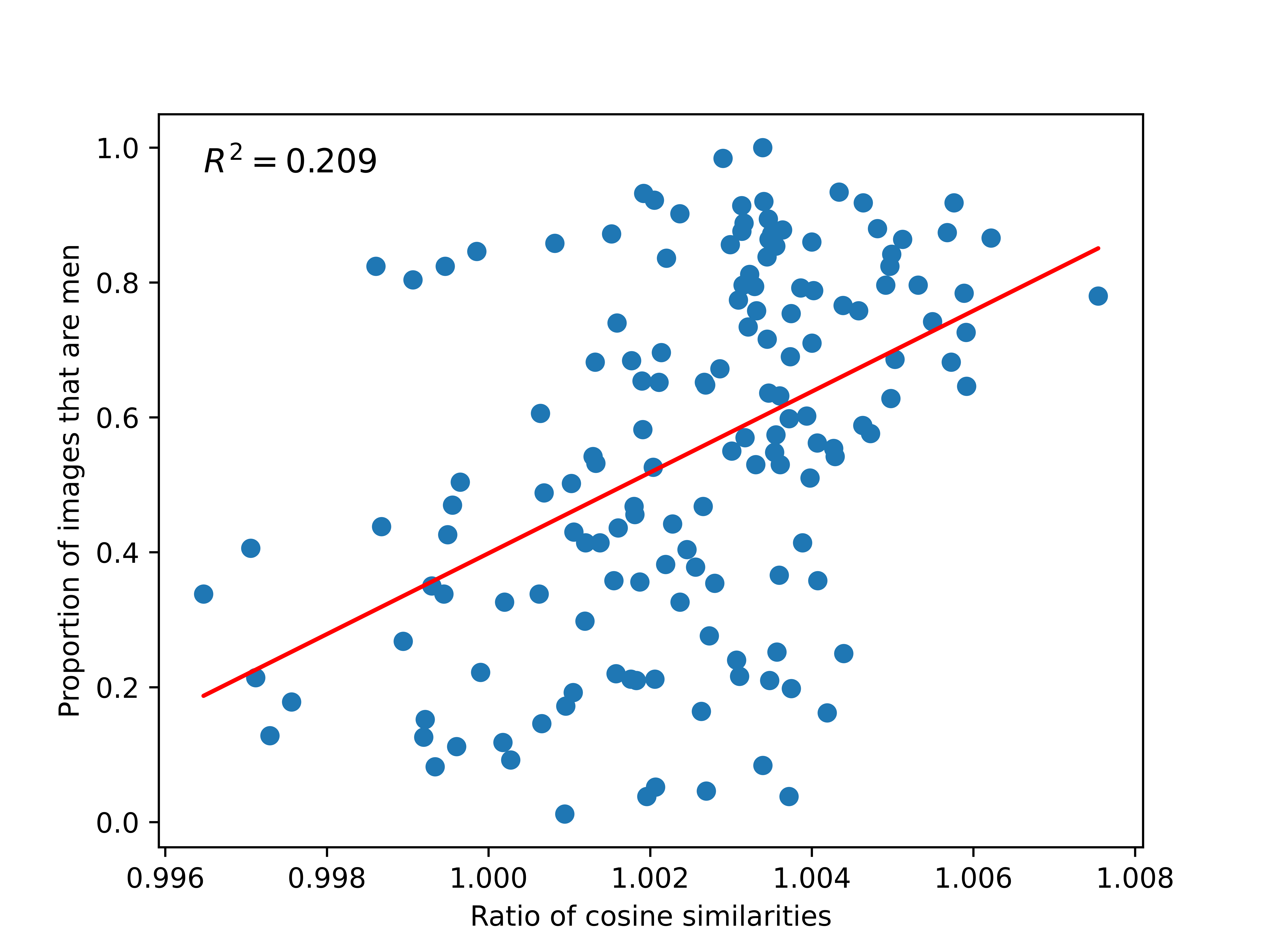
To provide empirical support for Theorem 4.5, we study gender bias in occupations for CLIP embeddings used as inputs for SD2.1 and images generated by SD2.1. We consider the Professions dataset containing portraits of people in 146 different professions from SD2.1 (Luccioni et al., 2023). For each profession, we compute the ratio of cosine similarity between the CLIP embeddings of the prompts “Profession, man” and “Profession,” and the cosine similarity of the CLIP embeddings of the prompts “Profession, woman” and “Profession.” If this ratio is above 1, then this profession is biased in embedding space towards men over woman. To measure the bias in SD2.1 outputs, we sort the image generations into men or women categories with CLIP-ViT-B/32. In Figure 1, there is a mild correlation between gender bias in CLIP embeddings and gender bias in image generations for a given occupation.
B.2 Additional Details of Diffusion-From-Scratch Training
To better disentangle whether our experimental results above are from a biased embedding or a biased set of training data, we train a conditional diffusion model from scratch with balanced training data across classes but with biased prompt embeddings. Using this model, we test whether generations from this model for a given biased prompt are imbalanced.
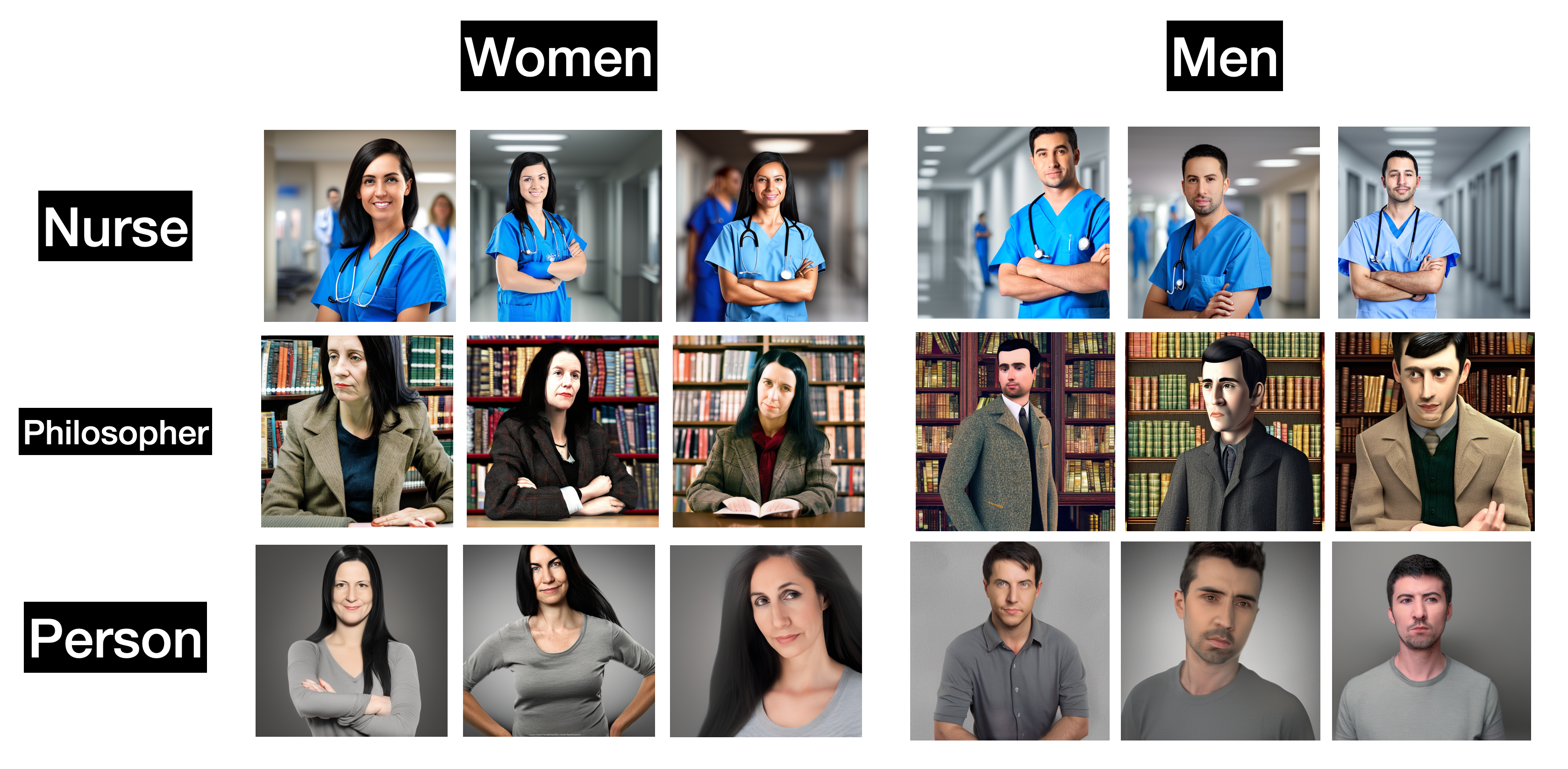
To probe this, we first took the the w2vNEWS embedding studied in (Bolukbasi et al., 2016), and in particular train our diffusion model on men and women in three categories: nurses (the second-highest female-biased occupation in (Bolukbasi et al., 2016)), philosophers (the fourth-highest male-biased occupation in (Bolukbasi et al., 2016)), and generic people. See Table 2 for the cosine similarities between these embeddings. Within each of these three categories, we trained on 12000 images, 6000 men and 6000 women. Because we cannot obtain these images organically, we made a synthetic dataset using Stable Diffusion. We highlight here that for each subject (nurse, philosopher, or generic person), we wanted man vs. woman to be the main difference in image distribution. As such, we controlled all generations to be white, with black hair, and have the same instructions (see below). This is not to say that there are no differences between classes; one thing we notice, for instance, is that the nurses appear much younger and the philosophers appear much older. For the purposes of our experiment, however, these differences are not important, as we only label men and women. We also note that we specify the clothing and background for each subject to be clearly recognizable, so that data is easy to label. For instance, a generated image with someone in blue scrubs is clearly a nurse, and a generated image with a library background is clearly a philosopher.
To operationalize our diffusion model, we implemented a conditional diffusion model from scratch based on public reference implementations, re-implemented core modules to handle our biased input embedding, and trained it on the 36000 images. Because of compute limitations, we could only train a model to output 64x64 images. See Section B.2.2 in the Appendix for full details on these changes.
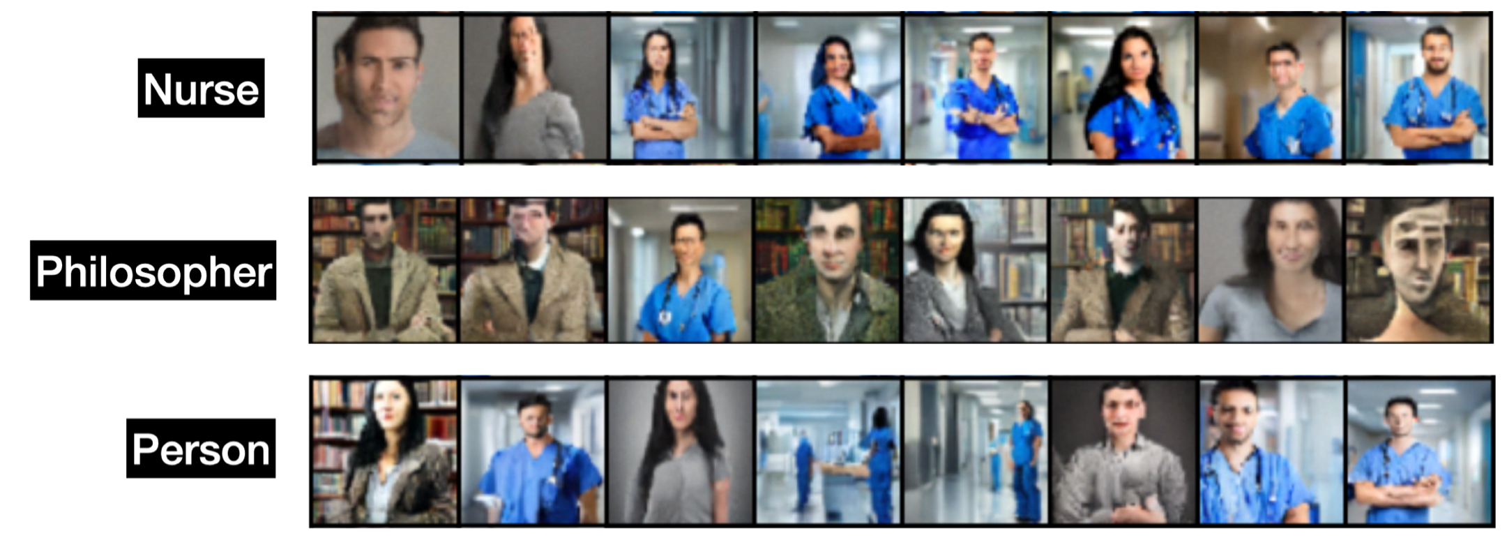
Data labeling was a challenge, because generated model images were small (64x64). Additionally, generation quality was somewhat poor at times (as one might expect with a bespoke model using synthetic data); for instance, some generated image did not contain an actual person. See Figure 3. As such, to label our data as man/woman, we first manually filtered generations for low quality (e.g. pictures where one cannot discern an actual person present), unidentifiable gender, or inconsistent occupation; then, we adopted a consensus-based approach with two reviewers to sort the image generations into men or women groups. For 170 generated images for the following three prompts (“nurse”, “person”, and “philosopher”), our consensus approach yielded 109 “nurse” images, 130 “philosopher” images, and 139 “person”” images.
Table 1 illustrates our results. We see that, even with a balanced set of training data, the majority of nurses were classified as women (59.6%) and the majority of philosophers were classified as men (55.4%). Simply generating an image conditioned on “person,” however, yields balanced representation. The frequency of men or women groups for both philosophers and nurses were both equal in the training data, but the diffusion model still exhibits a bias towards female nurses over male nurses and male philosophers over female philosophers. Because we controlled for imbalances in training data distribution in this experiment, this confirms our hypothesis that biased embeddings alone can cause biased outputs.
| Generation | Proportion |
|---|---|
| Nurse | 0.596 |
| Person | 0.504 |
| Philosopher | 0.446 |
| Nurse | Person | Philosopher | |
|---|---|---|---|
| Man | 0.255 | 0.534 | 0.290 |
| Woman | 0.441 | 0.547 | 0.176 |
B.2.1 Synthetic Data Generation.
To get 6000 images across six different classes, we used Stable Diffusion to create synthetic data. In general, we thought these images were high quality and could be used for our training pipeline; Figure 2 illustrates three random images from each of the six classes. Because our model is trained to generate 64x64 images, we then downscaled the output images to 64x64. The precise prompts used to generate 6000 images of each class are listed below:
-
•
Male Nurse: Create a realistic image of a male nurse standing confidently in the center of a modern hospital setting. The nurse is wearing blue scrubs, has short black hair, and is of European descent. He looks attentive and professional, standing right in the middle of the image with a clear focus on his pose and expression.
-
•
Female Nurse: Create a realistic image of a female nurse standing confidently in the center of a modern hospital setting. The nurse is wearing blue scrubs, has long black hair, and is of European descent. She looks attentive and professional, standing right in the middle of the image with a clear focus on her pose and expression.
-
•
Male Philosopher: Create a realistic photo image of a Caucasian male philosopher, situated in the center of a classic library background. He wears a tweed jacket and has short black hair, neatly styled. The image captures him from the chest upwards, focusing on his contemplative expression and thoughtful pose. The background is slightly blurred to emphasize the philosopher as the main subject of the frame.
-
•
Female Philosopher: Create a realistic photo image of a Caucasian female philosopher, positioned in the center of a library background. She wears a tweed jacket and has long black hair, neatly styled. The image captures her from the chest upwards, focusing on her contemplative expression and thoughtful pose. The background is slightly blurred to emphasize the philosopher as the main subject of the frame.
-
•
Man, Generic: Create a realistic photo image of a Caucasian man wearing a gray shirt, positioned in the center of a neutral background. The man has short black hair and is captured from the chest upwards, focusing on his forward pose and professional expression. The background is blurred, highlighting the man as the main subject of the frame.
-
•
Woman, Generic: Create a realistic photo image of a Caucasian woman wearing a gray shirt, positioned in the center of a neutral background. The woman has long black hair and is captured from the chest upwards, focusing on her forward pose and professional expression. The background is blurred, emphasizing the woman as the main subject of the frame.
B.2.2 Model Configuration.
Adding in our embedding. The base implementation of a conditional diffusion model that we base our implementation on takes as input to the UNet (the neural network that learns the score) some vector where , where is a sinusoidal positional encoding of the time and is an embedding of class (a number from 0 to 9) in 256-dimensional space that gets learned as the model runs. In our diffusion model, we changed the positional encoding of time to instead be of the form , and concatenate the positional encoding with a text embedding of the input prompt in . Since every embedding in w2vNEWS is in , we use a Johnson-Lindenstrauss projection to reduce its dimension to 128.
Training on Multiple Words. We use the w2vNEWS embedding here because (Bolukbasi et al., 2016) conducts a rigorous study of biases in this embedding, and we failed to find such a complete study for CLIP’s text embeddings. Because we could only condition on words in the embedding, however, mechanically we had to train every training sample/image on three words that labeled the image; see below:
-
•
Male Nurse: Man, Nurse, Person
-
•
Female Nurse: Woman, Nurse, Person
-
•
Male Philosopher: Man, Philosopher, Person
-
•
Female Philosopher: Woman, Philosopher, Person
-
•
Woman (Generic): Woman, Person, Woman
-
•
Man (Generic): Man, Person, Man
Appendix C Details from Section 4
C.1 Multicalibration
In Section 5.1, we define a notion of fairness based on the multiaccuracy framework. However, note that the protection offered by multiaccuracy in the example above is fairly weak. In particular, consider the case where , the true quality of images in and is (roughly) uniformly distributed between 0 and 1, and consider the auditing function
Note that is -multiaccurate since . However, clearly performs much worse on images of male doctors than female doctors. In particular, assuming that our generative model is reasonably good, we would expect all images generated for the prompt to have a true score , so our auditing function would consistently give male doctors a higher score than female doctors. Note that this issue can be partially aleviated by definining a richer class of images . However, it is also possible to define a stronger notion of fairness that avoids this issue.
Definition C.1 (Multicalibration).
Let be a collection of subsets of and . An auditing function is -multicalibrated for prompt if, for all and for all where ,
Note that multicalibration is equivalent to multiaccuracy with defined as the level sets of true alignment scores of the original subsets of images. Thus, this definition implicitly creates a richer class of images. Moreover, note that the example function defined above is not -multicalibrated for any , since for , . However, while this is a stronger notion of fairness, there are still ways in which a function that is -multicalibrated may behave differently on sets in ; for example, it is possible that a function that is -multicalibrated has more variance in its scores for images of female doctors than male doctors with some fixed true score .
C.2 Average-then-Score
Here, we define average-then-score, an alternative method for calculating alignment scores based on multimodal embeddings. In this approach, to calculate the alignment score of a model for a prompt , we start by sampling a set of images from . We then calculate We return the score scaled to . Note that the key difference is when we take the average - in the original approach, the average is taken after the scores are calculated, whereas here we take the average of the image embeddings before calculating the score. To understand why these differ, we show the following result.
theoremavgthenscore For a prompt and a set of images , if for all , average-then-score is lower bounded by score-then-average.
Proof.
We prove a more general result. Given unit vectors and , where for all , we show that
First, we see that
On the other hand, we see that
Finally, since , by triangle inequality we know that . Thus,
completing the proof.
To show the original theorem statement, for a prompt and a subset of images , consider and for all . Scaling the cosine similarity to does not affect the result, so the left side of the inequality is equivalent to score-then-average and the right side of the inequality is equivalent to average-then-score. ∎
Although this method still biased from the perspective of multiaccuracy, we provide some intuition on why it may reward models that output images with more balanced attributes. Consider a base prompt and attributes . Let be a subset of images corresponding to prompt with attribute , and let . Since the goal of the embedding space is to map prompts close to images that match it, we should expect that is close to for all . Thus, we should also expect that is positioned somewhere “between” the clusters of vectors corresponding to each subset of images, though this vector may be closer to some clusters than others. If this intuition is correct, averaging image vectors with more diverse attributes should bring us closer to the vector for the prompt than averaging image vectors with a single attribute, so our score function should reward some amount of diversity, though the exact ratios at which it is maximized may differ. We explore this hypothesis and evaluate this method in Section C.3.
One downside of using average-then-score over score-then-average is that it fails to take into account variance. In particular, a set of image vectors could combine to give a very high score because they happen to average in the same direction as the embedding of the prompt even though none are individually close to the prompt. Thus, if used in practice, it will be important to add a term that penalizes variance in the image vectors.
C.3 Evaluation Results
C.3.1 Text-Text Bias
As shown in Section 5.2, biases on attributes in the prompt embedding space imply bias for images close to the attributes in the image embedding space. Thus, we start by analyzing the bias present in the prompt embedding space of CLIP. Our results are shown in Table 3.
| Occupation | Male | Female | Delta | Average |
|---|---|---|---|---|
| firefighter | 0.971 | 0.919 | 0.052 | 0.959 |
| chemist | 0.962 | 0.923 | 0.039 | 0.955 |
| chef | 0.954 | 0.918 | 0.036 | 0.950 |
| architect | 0.957 | 0.924 | 0.033 | 0.955 |
| biologist | 0.978 | 0.949 | 0.029 | 0.972 |
| professor | 0.968 | 0.950 | 0.018 | 0.966 |
| doctor | 0.962 | 0.947 | 0.015 | 0.965 |
| teacher | 0.962 | 0.947 | 0.015 | 0.963 |
| librarian | 0.962 | 0.951 | 0.011 | 0.969 |
| hairdresser | 0.951 | 0.958 | -0.007 | 0.967 |
| receptionist | 0.954 | 0.962 | -0.008 | 0.970 |
| nurse | 0.951 | 0.973 | -0.022 | 0.974 |
We evaluate 12 occupations for bias on two genders - male and female. For every occupation , the male column shows the cosine similarity between the embedding of and the embedding of , and the female column shows the cosine similarity between the embedding of and the embedding of . The entries are sorted in increasing order of delta, the difference between the male and female similarity scores. We see that our results match several of the biases observed by (Bolukbasi et al., 2016). In particular, “nurse,” “receptionist” and “hairdresser” are she professions, while “doctor” and “architect” are he professions. The average column measures the cosine similarity between the embedding of and the average of the embeddings of and . It is interesting to note that these are always closer to the larger similarity score, and are sometimes larger than both. This motivates the average-then-score approach discussed in Section C.2 since we would hope that the image embeddings behave similarly.
C.3.2 Text Embedding Bias
In this section we investigate the bias in the similarities between occupation prompt vectors and image prompt vectors with specific genders. Our results are shown in Table 4.
| Occupation | Male | Female | Delta | Average |
|---|---|---|---|---|
| doctor | 0.800 | 0.780 | 0.020 | 0.801 |
| nurse | 0.772 | 0.833 | -0.061 | 0.813 |
We evaluate doctors and nurses for bias on two genders - male and female. To do so, we collect images of male doctors, female doctors, male nurses and female nurses manually from Google Images. We then calculate the average cosine similarity between the embedding of ‘doctor’ and the embeddings of all male and female medical professionals respectively. Next, we do the same for “nurse.” Note that the set of images is the same across both occupations, so there is no inherent difference in quality; by symmetry, we should expect that images of nurses are as close to the prompt “doctor” as images of doctors are to the prompt “nurse.” This is also why we restrict our attention to these two occupations; without the control of using the same sets of images for different professions, it is possible that the male pictures happen to be higher quality than the female pictures of vice-versa.
The delta column shows that for the same set of images, male medical professionals got a 0.02 higher score than female medical professionals on average for the prompt “doctor,” and a 0.061 lower score for the prompt “nurse.” Thus, this clearly demonstrates an underlying bias in the auditing CLIPScore function; models that generate only male doctors and only female nurses get over higher alignment scores.
The average column measures the cosine similarity between the occupation and the average of the embeddings of the male and female images. We see that the average of the images performs better than either individual gender for the prompt “doctor,” but lands somewhere in between for the prompt nurse. We explore the implications of this further in the next section.
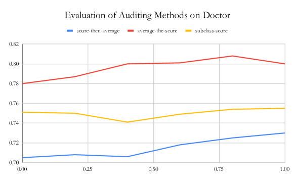
C.3.3 Mitigating Bias
In this section, we explore how our proposed auditing methods, average-then-score and subclass-score, compare to the original method score-then-average on the prompts “doctor” and “nurse.” The results are visualized in Figure 4. We find that average-then-score seems to perform roughly as well as score-then-average, biased towards male images for “doctor” and female images for “nurse.” However, subclass-score performs significantly better for both, staying roughly consistent as the gender ratio changes. Thus, subclass-score is the most promising step for alleviating gender bias in alignment scores for text-to-image models.