Dynamic landscapes and statistical limits on growth during cell fate specification

Abstract

The complexity of gene regulatory networks in multicellular organisms makes interpretable low-dimensional models highly desirable. An attractive geometric picture, attributed to Waddington, visualizes the differentiation of a cell into diverse functional types as gradient flow on a dynamic potential landscape, but it is unclear under what biological constraints this metaphor is mathematically precise. Here, we show that growth-maximizing regulatory strategies that guide a single cell to a target distribution of cell types are described by time-dependent potential landscapes, under certain generic growth-control tradeoffs. Our analysis leads to a sharp bound on the time it takes for a population to grow to a target distribution of a certain size. We show how the framework can be used to compute Waddington-like epigenetic landscapes and growth curves in an illustrative model of growth and differentiation. The theory suggests a conceptual link between nonequilibrium thermodynamics and cellular decision-making during development.

Organismal development is a tremendously complex process involving the coordinated growth and differentiation of a single cell into a well-defined population of cell types. During cell fate specification, the re-organization of gene expression profiles is coordinated by complex regulatory mechanisms that parse external signals and control the expression of hundreds to thousands of genes [1, 2, 3]. Both contextual instructive signals and stochastic factors influence the eventual fates of a cell and its descendants [4, 5, 6].

One would hope that cellular processes involved in cell fate specification can be described by interpretable models that reflect core regulatory principles and guide new experiments. One such intuitive picture, provided by Waddington, is that of a ball (an undifferentiated cell) rolling down a dynamic potential landscape with a “valley” bifurcating into multiple valleys, corresponding to the distinct fates that the cell can acquire [7, 8]. Under what physiological and functional constraints is this metaphor a mathematically precise description of cellular decision-making? One perspective emphasizes the structural stability property of gradient-like dynamical systems to motivate Waddington-like low-dimensional models of cell fate decisions [9, 10, 11, 12, 13]. A related static picture views cell types as attractors in energy-based models of associative memory [14, 15, 16].

Another perspective is provided by optimal transport [17, 18], which offers a powerful computational framework for tracing single-cell gene expression profiles over time [19, 20, 21]. Conceptually, optimal transport considers the context-dependent transformation of an initial distribution of cell states to a final distribution of cell states. Different optimal transport formulations correspond to different assumptions on the biological cost of transforming cell states.

The celebrated Benamou-Brenier theorem [22, 23] bridges these two perspectives by showing that under certain quadratic transport costs, the optimal transport map is described by gradient flow on a time-dependent potential landscape. However, it is unclear how quadratic (or other) costs on transport maps relate to physiologically relevant constraints, bringing into question the interpretation of maps inferred by optimal transport. Moreover, growth is central to development. Existing frameworks either ignore growth or relax the hard requirement that mass is conserved to a soft constraint when analyzing data [24, 19].

In this Letter, we consider a population of non-interacting cells growing into an arbitrary target distribution of cell states in a finite time while maximizing growth. An example is presented in Figure 1. Our two main results are an analog of the Benamou-Brenier result for a certain class of growth-control tradeoffs, which identifies mathematical constraints under which a Waddington-like picture is valid, and a precise statistical bound on population growth rate analogous to speed limits in nonequilibrium thermodynamics. The modeling framework is generally applicable to scenarios where diversifying into a heterogeneous population conflicts with maximizing instantaneous growth. Examples include microbial bet-hedging in unpredictable environments [25, 26], and the rapid proliferation and differentiation of cells into specialized types during inflammation and wound healing [27]. The framework further motivates the development of computational transport methods that incorporate physiologically relevant constraints. A notable departure from existing approaches is that gene regulation has a direct impact on growth, and all transport costs are built into this tradeoff.

We assume each cell has a state $\bm{g}$ (for example, its gene expression profile) which evolves as

$$dg_{\mu}=\left(f_{\mu}(\bm{g},t)+v_{\mu}(\bm{g},t)\right)dt+\sigma_{\mu\nu}dW_{\nu},$$ (1)

where $\mu$ indexes the components of $\bm{g}$, $f_{\mu}(\bm{g},t)$ describes the passive dynamics of $g_{\mu}$ (for example, dilution and degradation), $v_{\mu}(\bm{g},t)$ is the regulatory control variable and $dW_{\mu}$ is a Wiener process that represents noise due to stochastic gene expression and other factors (note $\langle dW_{\mu}(t)\rangle=0$, $\langle dW_{\mu}(t)dW_{\nu}(t^{\prime})\rangle=\delta_{\mu\nu}\delta(t-t^{\prime})dt$ and Einstein summation is used throughout). Here, time $t$ represents the time since an external triggering event, but in general reflects the influence of a time-varying external signal on gene regulation $\bm{v}$.

The cell doubles with a probability per unit time (i.e., growth rate) $\gamma(\bm{g},\bm{v})$, where the dependence on $\bm{g}$ and $\bm{v}$ reflects the fact that a cell’s growth rate depends on how much of the proteome is devoted to protein synthesis and the fraction of the synthesis machinery that is occupied by the synthesis of proteins that do not contribute towards further synthesis. We consider terms to second-order in $\bm{v}$:

$$\gamma(\bm{g},\bm{v})=\gamma_{0}(\bm{g})+d_{\mu}(\bm{g})v_{\mu}+\frac{1}{2}h_{\mu\nu}(\bm{g})v_{\mu}v_{\nu},$$ (2)

where $\gamma_{0}(\bm{g})$ and $d_{\mu}(\bm{g})$ are arbitrary functions of $\bm{g}$ and $h_{\mu\nu}$ is symmetric with additional constraints discussed further below. $d_{\mu}$ is set to zero by noting that it can be recovered by an appropriate translation of $f_{\mu},v_{\mu}$ and $\gamma_{0}$. A cell’s progeny when it doubles inherit the same state as their parent but their states will subsequently diverge due to noise (Figure 1).

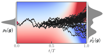
Figure 1: We consider the growth of a cell with a multi-dimensional cellular state $\bm{g}$ from an arbitrary probability density $\rho_{0}(\bm{g})$ to a population with arbitrary target density $\rho^{\dagger}_{T}(\bm{g})$ in finite time $T$. Here, a single cell replicates and its descendants acquire distinct fates due to stochasticity in cellular state dynamics. The regulatory control $v(g,t)$ is shown in red ($v>0$) and blue ($v<0$).

We aim to find the growth-maximizing regulatory strategy $\bm{v}^{*}(\bm{g},t)$ that guides a population of non-interacting cells with an arbitrary (but known) initial probability density $\rho_{0}(\bm{g})$ to an arbitrary target probability density $\rho^{\dagger}_{T}(\bm{g})$ in finite time $T$. We formulate the problem as inverse control, where we hope to find a terminal “reward” function $\omega(\bm{g})$ such that at optimality the normalized density at $T$ is precisely the target distribution $\rho^{\dagger}_{T}(\bm{g})$ [28, 29]. If such a reward function and corresponding optimal strategy is found, the expected reward is $N_{T}^{*}\int\rho^{\dagger}_{T}(\bm{g})\omega(\bm{g})d\bm{g}$, where $N_{T}^{*}$ is the number of cells at time $T$. Since the optimal strategy maximizes reward, it is also the one that maximizes average growth rate $\Gamma^{*}_{T}=T^{-1}\log N_{T}^{*}$ amongst the class of strategies that guide a population from $\rho_{0}(\bm{g})$ to $\rho^{\dagger}_{T}(\bm{g})$.

We begin by defining $w(\bm{g},t)$ as the expected future reward of a cell with state $\bm{g}$ at time $t$, commonly known in sequential optimization as the value function. A dynamic programming equation relates $w(\bm{g},t)$ with its expected value at $t+dt$ given the optimal control at that state:

$$w(\bm{g},t)=\max_{\bm{v}}\left\{\left(1+\gamma(\bm{g},\bm{v})dt\right)\langle w(\bm{g}+d\bm{g},t+dt)\rangle\right\},$$ (3)

where the expectation is over noise $dW_{\mu}$ and the growth term takes into account the probability that the cell doubles in interval $dt$. We expand $w(\bm{g}+d\bm{g},t+dt)$ in a Taylor series, compute expected values and retain terms of order $dt$ to get

$$\max_{\bm{v}}\left(\partial_{t}w+\left(f_{\mu}+v_{\mu}\right)\partial_{\mu}w+\frac{1}{2}\Sigma_{\mu\nu}\partial^{2}_{\mu\nu}w+\gamma w\right)=0,$$ (4)

where $\Sigma_{\mu\nu}=\sigma_{\mu\mu^{\prime}}\sigma_{\nu\mu^{\prime}}$. We have dropped the $\bm{g},t$ arguments for convenience and a standard notation for partial derivatives is used ($\partial_{\mu}=\partial/\partial g_{\mu}$, etc., unless specified otherwise). For $\gamma$ quadratic in $v_{\mu}$, taking the max over $v_{\mu}$ we get $v_{\mu}^{*}=-h^{-1}_{\mu\nu}\partial_{\nu}\log w$. Plugging this back in (4), leads to the nonlinear PDE

$$\partial_{t}w+f_{\mu}\partial_{\mu}w-\frac{1}{2w}h^{-1}_{\mu\nu}(\partial_{\mu}w)(\partial_{\nu}w)+\frac{1}{2}\Sigma_{\mu\nu}\partial^{2}_{\mu\nu}w+\gamma_{0}w=0.$$ (5)

Consider a substitution $\psi=w^{1+1/\alpha}$, where $\alpha>0$ is a constant. This yields a linear PDE in $\psi$ if $(h\Sigma)_{\mu\nu}=-\alpha\delta_{\mu\nu}$. Intuitively, this constraint requires that the magnitude of gene expression noise is inversely proportional to the cost of expressing the gene and that there is a single constant $\alpha$ that scales gene expression cost. The condition further implies $\Sigma_{\mu\nu}$ is full rank and $h$ is independent of $\bm{g}$. We then have

$$\partial_{t}\psi+f_{\mu}\partial_{\mu}\psi+\frac{1}{2}\Sigma_{\mu\nu}\partial^{2}_{\mu\nu}\psi+\gamma_{0}\left(\frac{1+\alpha}{\alpha}\right)\psi=0.$$ (6)

Using the Feynman-Kac formula, the solution can be expressed in terms of an uncontrolled process with drift $\bm{f}$, diffusion tensor $\Sigma/2$ and growth rate $\gamma_{0}\left(\frac{1+\alpha}{\alpha}\right)$. Specifically, if the transition density of this uncontrolled process is $\phi(\bm{g},t;\bm{g}^{\prime},t^{\prime})$ for $t\geq t^{\prime}$ (with boundary condition $\phi(\bm{g},t^{\prime};\bm{g}^{\prime},t^{\prime})=\delta(\bm{g}-\bm{g}^{\prime})$), we have

$$\psi(\bm{g},t)=\int d\bm{g}^{\prime}\phi(\bm{g}^{\prime},T;\bm{g},t)\psi(\bm{g}^{\prime},T),$$ (7)

where $\psi(\bm{g},T)=\omega(\bm{g})^{1+1/\alpha}$ from our definition of $\psi$. Define $\hat{\psi}(\bm{g},t)$ as

$$\hat{\psi}(\bm{g},t)=\int d\bm{g}^{\prime}\phi(\bm{g},t;\bm{g}^{\prime},0)\hat{\psi}(\bm{g}^{\prime},0).$$ (8)

$\hat{\psi}$ satisfies the Kolmogorov forward equation [30]

$$\partial_{t}\hat{\psi}+\partial_{\mu}\left(f_{\mu}\hat{\psi}\right)-\frac{1}{2}\Sigma_{\mu\nu}\partial^{2}_{\mu\nu}\hat{\psi}-\gamma_{0}\left(\frac{1+\alpha}{\alpha}\right)\hat{\psi}=0,$$ (9)

which is also the forward equation satisfied by $\phi$. We now ask if the (unnormalized) density $\rho(\bm{g},t)$ of the optimally controlled process can be expressed in terms of $\psi$ and $\hat{\psi}$. From (1) and (2), $\rho$ satisfies the forward equation

$$\partial_{t}\rho+\partial_{\mu}\left((f_{\mu}+v^{*}_{\mu})\rho\right)-\frac{1}{2}\Sigma_{\mu\nu}\partial^{2}_{\mu\nu}\rho-\gamma_{0}\rho-\frac{1}{2}h_{\mu\nu}v_{\mu}^{*}v_{\nu}^{*}\rho=0,$$ (10)

with optimal control (expressed in $\psi$)

$$v_{\mu}^{*}=(1+\alpha)^{-1}\Sigma_{\mu\nu}\partial_{\nu}\log\psi.$$ (11)

We consider the ansatz

$$\rho(\bm{g},t)=\hat{\psi}(\bm{g},t)\psi(\bm{g},t)^{\frac{1}{1+\alpha}},$$ (12)

and using (6), (9), it is lengthy but straightforward to verify through direct substitution that (12) satisfies (10).

In summary, the density $\rho$ of the optimally controlled process is given by (12) in terms of $\psi$ and $\hat{\psi}$, which in turn satisfy (6), (9) respectively, and the boundary conditions

$$\rho_{0}(\bm{g}) =\hat{\psi}(\bm{g},0)\psi(\bm{g},0)^{\frac{1}{1+\alpha}},$$ (13)

$$N_{T}^{*}\rho_{T}^{\dagger}(\bm{g}) =\hat{\psi}(\bm{g},T)\psi(\bm{g},T)^{\frac{1}{1+\alpha}}.$$ (14)

Given a solution $\psi$ of the above set of equations, the optimal control is the gradient of a time-dependent potential (11). However, it is unclear whether solutions exist for arbitrary boundary conditions (13), (14). In the special case $\gamma_{0}=0$ and $\alpha\to 0$, our set of equations are identical to the equations obtained in entropy-regularized optimal transport, also known as the Schrödinger bridge problem [31, 32, 28, 29]. Solutions exist for general boundary conditions and can be found using a simple procedure known as iterative proportional fitting or the Sinkhorn algorithm [33, 34, 35, 36], which begins with an initial guess for $\hat{\psi}$ and iteratively updates (13), (14) using (7), (8). Whether an analogous procedure can be derived for our case is beyond the scope of this paper.

A statistical bound on growth. $N_{T}^{*}$, or equivalently, the average growth rate $\Gamma^{*}_{T}$ is self-consistently determined by the set of equations above for a given target $\rho_{T}^{\dagger}$. A more interpretable form is obtained when $\Gamma^{*}_{T}$ is expressed in terms of the average growth rate $\Gamma_{T}^{\max}$ of a population (with initial density $\rho_{0}$) where the control is chosen to maximize growth over time $T$ with no constraint on the final density. The solution for this growth-maximizing process is obtained by setting $\omega(\bm{g})=\psi(\bm{g},T)^{\frac{\alpha}{1+\alpha}}=c>0$, i.e., a constant positive reward $c$ is given for each cell at time $T$. $\Gamma_{T}^{\max}$ can be expressed in terms of

$$\bar{\nu}_{T}(\bm{g}) =\frac{1}{T}\int_{0}^{T}\nu(t;\bm{g})dt,\text{ where}$$

$$\quad\nu(t;\bm{g}) =\int d\bm{g}^{\prime}\gamma_{0}(\bm{g}^{\prime})\tilde{\phi}(\bm{g}^{\prime},t;\bm{g},0)$$ (15)

is the instantaneous growth rate and $\tilde{\phi}$ is the normalized $\phi$ (Appendix A). Specifically,

$$\Gamma^{\max}_{T}=\frac{1}{T}\log\int d\bm{g}\rho_{0}(\bm{g})e^{T\bar{\nu}_{T}(\bm{g})}.$$ (16)

Plugging in $\rho_{0}(\bm{g})=\delta(\bm{g}-\bm{g}_{0})$ in the above expression shows that $\bar{\nu}_{T}(\bm{g}_{0})$ is to be interpreted as the average growth rate of the growth-maximizing population that begins from a single cell with state $\bm{g}_{0}$ and that $\phi(\bm{g},t;\bm{g}_{0},0)$ describes the time evolution of this process.

Multiplying both sides of (13) by $e^{T\bar{\nu}_{T}(\bm{g})}$, integrating over $\bm{g}$ and using (16), (7), (14) (see Appendix A), we get

$$\Gamma_{T}^{*}=\Gamma^{\max}_{T}-\frac{K_{\alpha}(\rho^{\dagger}_{T}||\rho^{\max}_{T})}{T},$$ (17)

where

$$K_{\alpha}(\rho_{T}^{\dagger}||\rho^{\max}_{T}) \equiv\log\int d\bm{g}e^{T\bar{\nu}_{T}(\bm{g})}\hat{\psi}(\bm{g},0)\xi(\bm{g})^{\frac{1}{1+\alpha}},$$ (18)

$$\xi(\bm{g}) =\int d\bm{g}^{\prime}\phi(\bm{g}^{\prime},T;\bm{g},0)\left(\frac{\rho^{\dagger}_{T}(\bm{g}^{\prime})}{\hat{\psi}(\bm{g}^{\prime},T)}\right)^{1+\alpha},$$

and $\rho^{\max}_{T}$ is the density at time $T$ if cells solely maximized growth beginning from $\rho_{0}$. Since the optimally controlled process specified by (12) is the one that maximizes growth rate amongst the class of control strategies that transform the population of cells from $\rho_{0}$ to $\rho_{T}^{\dagger}$, (17) provides an upper bound on the average growth rate over all such control strategies.

An application of Jensen’s inequality shows that $K_{\alpha}(\rho_{T}^{\dagger}||\rho^{\max}_{T})\geq 0$ and equals zero only if $\rho^{\dagger}_{T}=\rho^{\max}_{T}$ (Appendix A). $K_{\alpha}$ thus appears to behave like a statistical divergence that measures the distance between the target density and the density at time $T$ if cells solely maximized growth. This interpretation is more transparent for the case when the developmental process begins from a single cell at $t=0$, which we now consider.

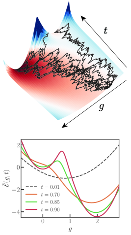
Figure 2: (Top) Sample trajectories on a one-dimensional time-varying potential landscape $\tilde{\mathcal{E}}$ differentiating into two cell types in a 1:4 ratio. Here $\tilde{\mathcal{E}}=\mathcal{E}+g^{2}/2-t$ with $T=1,\gamma_{b}=1,\lambda^{2}=0.1,\alpha=0.1$. (Bottom) The landscape bifurcates from one stable state to two stable states at $t/T\approx 0.8$.

Growth from a single cell. An exact solution is obtained when the initial distribution is $\rho_{0}(\bm{g})=\delta(\bm{g}-\bm{g}_{0})$, i.e., growth from a single cell with initial state $\bm{g}_{0}$. In this case, $\hat{\psi}$ with

$$\hat{\psi}(\bm{g},t)=\phi(\bm{g},t;\bm{g}_{0},0)/\psi(\bm{g}_{0},0)^{\frac{1}{1+\alpha}},$$ (19)

satisfies the initial condition (13) (since $\phi(\bm{g},t^{\prime};\bm{g}^{\prime},t^{\prime})=\delta(\bm{g}-\bm{g}^{\prime})$) and the forward equation (9). From (12), the final distribution is

$$\rho(\bm{g},T)=\phi(\bm{g},T;\bm{g}_{0},0)\left(\frac{\psi(\bm{g},T)}{\psi(\bm{g}_{0},0)}\right)^{\frac{1}{1+\alpha}}.$$ (20)

Enforcing $\rho(\bm{g},T)\propto\rho^{\dagger}_{T}(\bm{g})$ simply requires choosing $\omega(\bm{g})$ such that

$$\psi(\bm{g},T)=\omega(\bm{g})^{\frac{1+\alpha}{\alpha}}=\left(\frac{\rho^{\dagger}_{T}(\bm{g})}{\phi(\bm{g},T;\bm{g}_{0},0)}\right)^{1+\alpha}.$$ (21)

From (7) and (11), the flow is then specified by a time-dependent potential $\mathcal{E}\equiv-(1+\alpha)^{-1}\log\psi$, i.e.,

$$\mathcal{E}(\bm{g},t)=-\frac{1}{1+\alpha}\log\int d\bm{g}^{\prime}\phi(\bm{g}^{\prime},T;\bm{g},t)\left(\frac{\rho^{\dagger}_{T}(\bm{g}^{\prime})}{\phi(\bm{g}^{\prime},T;\bm{g}_{0},0)}\right)^{1+\alpha}.$$ (22)

The expression (18) for $K_{\alpha}$ reduces to

$$K_{\alpha}(\rho_{T}^{\dagger}||\rho^{\max}_{T})=\frac{\alpha}{1+\alpha}D_{1+\alpha}(\rho_{T}^{\dagger}||\rho^{\max}_{T}),$$ (23)

where $D_{1+\alpha}(\rho_{T}^{\dagger}||\rho^{\max}_{T})$ is the Rényi divergence [37] with parameter $1+\alpha$ and $\rho^{\max}_{T}(\bm{g})=\tilde{\phi}(\bm{g},T;\bm{g}_{0},0)$. The well-known Kullback-Leibler divergence is recovered in the limit $\alpha\to 0$.

A 1D model of growth and differentiation. We illustrate our computational framework using a simplified one-dimensional model of growth and differentiation. We consider a single cell with initial state $g_{0}=0$ developing in time $T$ into a mixture of two Gaussians with means 0 and $\theta$. Cell state dynamics are given by

$$dg=-gdt+v(g,t)dt+dW,$$ (24)

with growth rate $\gamma(g,v)=\gamma_{b}-\frac{1}{2}\lambda^{2}g^{2}-\frac{1}{2}\alpha v^{2}$ for constants $\gamma_{b},\lambda,\alpha$. This models the growth and diversification of a cell into a mixture of a fast-growing cell type ($g=0$) and a slow-growing cell type ($g=\theta>0$). The negative feedback term in (24) represents dilution and degradation of the marker gene $g$ and time is re-scaled by the timescale of dilution/degradation.

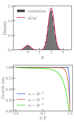
Figure 3: (Top) Samples from the 1D model match the target density. Here $\alpha=0.1,\lambda^{2}=0.25,\gamma_{b}=1$. (Bottom) Instantaneous population growth rates $\langle\gamma(g,v^{*})\rangle_{g\sim\rho(.,t)}$ for different values of $\alpha$. For small values of $\alpha$, the growth and differentiation phases are clearly delineated. The black dashed curve shows $\gamma(0,0)=\gamma_{b}=1$.

The transition density $\phi$ has an analytical expression (Appendix B), and the landscape can be numerically evaluated for an arbitrary target density $\rho_{T}^{\dagger}$ using (22). Figure 2 shows sample trajectories on a representative potential landscape. The landscape is smooth and displays a bifurcation from a single stable state to two stable states at late times (Figure 2, bottom). Samples from this process match the target density (Figure 3, top). The instantaneous growth rates for different $\alpha$ delineate two distinct phases of growth and differentiation for smaller $\alpha$ (Figure 3, bottom). The optimal control optimizes for growth for most of the interval and differentiates close to the end by rapidly ramping up expression of $g$, which is cheaper in the long-run when $\alpha\ll 1$.

Conclusion. A longstanding challenge in biological physics is to build interpretable, quantitative models of complex cellular regulatory processes that reflect general biological principles. Recent work has made progress towards this goal by describing experimental data using the language of dynamical systems theory, which emphasizes global geometric features at the expense of molecular details. An underlying assumption is that gene regulatory dynamics can be described using relatively simple gradient-like dynamics. Here, we show that regulatory circuits that maximize growth during cellular diversification indeed correspond to gradient flow on a potential landscape under certain assumptions on how gene regulation impacts growth. In deriving this result, we have ignored various important aspects of development, including intercellular communication and spatial structure. A general framework that incorporates these features remains elusive, though analogies between development processes and high-dimensional generative modeling offer some hope that this is feasible.

Our theory has close connections with optimal transport, and the Benamou-Brenier formalism in particular. The quadratic control transport cost considered in the Benamou-Brenier formalism directly relates to entropy produced during a nonequilibrium process, establishing a connection between optimal transport and stochastic thermodynamics [38, 39, 40]. Like the Benamou-Brenier formalism, we identify a set of constraints under which finding a transport map reduces to finding an appropriate time-dependent potential. Our results appear identical in the special case of $\gamma_{0}(\bm{g})=0,\alpha\to 0$, though further analysis is required to clarify the relationship between these two formalisms and unbalanced variants of optimal transport [24]. This connection also opens up the possibility of fitting single-cell gene expression data using growth-informed transport costs that naturally incorporate growth and offer a clearer biological interpretation.

Appendix A Derivation of eq. (17)

We first consider a process where the control variable $\bm{v}$ is chosen to maximize the average growth rate over time $T$ with initial density $\rho_{0}(\bm{g})$ and with no constraint on the final density. We will use a prime symbol to distinguish this growth-maximizing process from our original one. The solution to this process is obtained by setting $\omega^{\prime}(\bm{g})=1$ (or any positive constant). Note that it is only the boundary conditions for $\psi^{\prime}$ and $\hat{\psi}^{\prime}$ that change and not their equations. Also note that $\phi$ remains the same.

Since $\psi^{\prime}=w^{\prime 1+1/\alpha}$, $\omega(\bm{g})=1$ corresponds to the boundary condition $\psi^{\prime}(\bm{g},T)=1$ for all $\bm{g}$. Let

$$\bar{N}_{t}(\bm{g})\equiv\int d\bm{g}^{\prime}\phi(\bm{g}^{\prime},t;\bm{g},0).$$ (25)

From (7), since $\psi^{\prime}(\bm{g},T)=1$, we have $\psi^{\prime}(\bm{g},t)=\bar{N}_{T-t}(\bm{g})$ and in particular $\psi^{\prime}(\bm{g},0)=\bar{N}_{T}(\bm{g})$. From (14), the density at $T$ is $\hat{\psi}^{\prime}(\bm{g},T)$, which from (8) is given by

$$\hat{\psi}^{\prime}(\bm{g},T) =\int d\bm{g}^{\prime}\phi(\bm{g},T;\bm{g}^{\prime},0)\hat{\psi}^{\prime}(\bm{g}^{\prime},0),$$

$$=\int d\bm{g}^{\prime}\phi(\bm{g},T;\bm{g}^{\prime},0)\left(\frac{\rho_{0}(\bm{g}^{\prime})}{\bar{N}_{T}(\bm{g}^{\prime})^{\frac{1}{1+\alpha}}}\right)$$ (26)

The number of cells at time $T$ for the growth-maximizing process is

$$N_{T}^{\max} =\int d\bm{g}\rho(\bm{g},T)$$

$$=\int d\bm{g}\hat{\psi}^{\prime}(\bm{g},T)$$

$$=\int d\bm{g}^{\prime}\rho_{0}(\bm{g}^{\prime})\bar{N}_{T}(\bm{g}^{\prime})^{\frac{\alpha}{1+\alpha}},$$ (27)

where we have used (14) in the first step and (26), (25) in the second step when integrating over $\bm{g}$.

We can express $\bar{N}_{t}(\bm{g})$ in terms of a growth rate. Since $\phi$ satisfies (9), integrating both sides of (9) over $\bm{g}$ and setting boundary terms at $\pm\infty$ to zero, we have

$$\frac{d\bar{N}_{t}(\bm{g})}{dt} =\left(\frac{1+\alpha}{\alpha}\right)\int d\bm{g}^{\prime}\gamma_{0}(\bm{g}^{\prime})\phi(\bm{g}^{\prime},t;\bm{g},0)$$

$$=\left(\frac{1+\alpha}{\alpha}\right)\bar{N}_{t}(\bm{g})\int d\bm{g}^{\prime}\gamma_{0}(\bm{g}^{\prime})\tilde{\phi}(\bm{g}^{\prime},t;\bm{g},0),$$

$$=\left(\frac{1+\alpha}{\alpha}\right)\bar{N}_{t}(\bm{g})\nu(t;\bm{g})$$ (28)

where we have defined the normalized density $\tilde{\phi}$ and $\nu(t;\bm{g})$ is the population averaged growth rate for the uncontrolled process given that the population began at $t=0$ from a single cell with state $\bm{g}$:

$$\nu(t;\bm{g})\equiv\int d\bm{g}^{\prime}\gamma_{0}(\bm{g}^{\prime})\tilde{\phi}(\bm{g}^{\prime},t;\bm{g},0)$$ (29)

Integrating (28), we get

$$\frac{1}{T}\log\bar{N}_{T}(\bm{g}) =\left(\frac{1+\alpha}{\alpha}\right)\left(\frac{1}{T}\int_{0}^{T}\nu(t;\bm{g})dt\right)$$

$$\equiv\left(\frac{1+\alpha}{\alpha}\right)\bar{\nu}_{T}(\bm{g}).$$ (30)

Plugging the above expression for $\bar{N}_{T}(\bm{g})$ into (27), we get

$$\Gamma^{\max}_{T}=\frac{1}{T}\log N_{T}^{\max}=\frac{1}{T}\log\int d\bm{g}\rho_{0}(\bm{g})e^{T\bar{\nu}_{T}(\bm{g})}.$$ (31)

We now express the average growth rate $\Gamma^{*}_{T}=T^{-1}\log N_{T}^{*}$ of the optimally controlled process in terms of $\Gamma^{\max}_{T}$ and the divergence $K_{\alpha}$ defined in the main text. We return to the original process in $\psi$ and $\hat{\psi}$. Plugging in $\rho_{0}(\bm{g})=\hat{\psi}(\bm{g},0)\psi(\bm{g},0)^{\frac{1}{1+\alpha}}$ into the right hand side of (31), we have

$$\int d\bm{g}\rho_{0}(\bm{g})e^{T\bar{\nu}_{T}(\bm{g})}=\int d\bm{g}e^{T\bar{\nu}_{T}(\bm{g})}\hat{\psi}(\bm{g},0)\psi(\bm{g},0)^{\frac{1}{1+\alpha}},$$ (32)

$$=\int d\bm{g}e^{T\bar{\nu}_{T}(\bm{g})}\hat{\psi}(\bm{g},0)\left(\int d\bm{g}^{\prime}\phi(\bm{g}^{\prime},T;\bm{g},0)\left(\frac{N_{T}^{*}\rho^{\dagger}_{T}(\bm{g}^{\prime})}{\hat{\psi}(\bm{g}^{\prime},T)}\right)^{1+\alpha}\right)^{\frac{1}{1+\alpha}}$$ (33)

$$=N_{T}^{*}\int d\bm{g}e^{T\bar{\nu}_{T}(\bm{g})}\hat{\psi}(\bm{g},0)\xi(\bm{g})^{\frac{1}{1+\alpha}},$$ (34)

where we have used (7), (14) in the second step and defined

$$\xi(\bm{g})\equiv\int d\bm{g}^{\prime}\phi(\bm{g}^{\prime},T;\bm{g},0)\left(\frac{\rho^{\dagger}_{T}(\bm{g}^{\prime})}{\hat{\psi}(\bm{g}^{\prime},T)}\right)^{1+\alpha}.$$ (35)

Re-arranging and expressing in terms of growth rates,

$$\Gamma_{T}=\Gamma_{T}^{\max}-\frac{K_{\alpha}(\rho^{\dagger}||\rho^{\max})}{T}$$ (36)

where

$$K_{\alpha}(\rho_{T}^{\dagger}||\rho^{\max})\equiv\log\int d\bm{g}e^{T\bar{\nu}_{T}(\bm{g})}\hat{\psi}(\bm{g},0)\xi(\bm{g})^{\frac{1}{1+\alpha}}.$$ (37)

To show $K_{\alpha}(\rho_{T}^{\dagger}||\rho^{\max})\geq 0$, we rewrite the above expression in terms of normalized densities. We have $\phi(\bm{g}^{\prime},T;\bm{g},0)=\bar{N}_{T}(\bm{g})\tilde{\phi}(\bm{g}^{\prime},T;\bm{g},0)$ and express $\hat{\psi}$ in terms of its normalized density, $\hat{\psi}(\bm{g}^{\prime},T)=\hat{N}_{T}\hat{\psi}_{n}(\bm{g}^{\prime},T)$, where the normalization factor is

$$\hat{N}_{T} =\int d\bm{g}^{\prime}\hat{\psi}(\bm{g}^{\prime},T)$$

$$=\int d\bm{g}^{\prime}\int d\bm{g}\phi(\bm{g}^{\prime},T;\bm{g},0)\hat{\psi}(\bm{g},0)$$

$$=\int d\bm{g}\bar{N}_{T}(\bm{g})\hat{\psi}(\bm{g},0).$$ (38)

Using $\log\bar{N}_{T}(\bm{g})=\left(\frac{1+\alpha}{\alpha}\right)T\bar{\nu}_{T}(\bm{g})$, we have

$$K_{\alpha}(\rho_{T}^{\dagger}||\rho^{\max}) =\log\int d\bm{g}\bar{N}_{T}(\bm{g})^{\frac{\alpha}{1+\alpha}}\hat{\psi}(\bm{g},0)\xi(\bm{g})^{\frac{1}{1+\alpha}}$$

$$=\log\int d\bm{g}\frac{\bar{N}_{T}(\bm{g})\hat{\psi}(\bm{g},0)}{\int d\bm{g}^{\prime\prime}\bar{N}_{T}(\bm{g}^{\prime\prime})\hat{\psi}(\bm{g}^{\prime\prime},0)}\tilde{\xi}(\bm{g})^{\frac{1}{1+\alpha}},$$

$$=\log\int d\bm{g}Q(\bm{g})\tilde{\xi}(\bm{g})^{\frac{1}{1+\alpha}},$$ (39)

where we have defined

$$Q(\bm{g}) \equiv\frac{\bar{N}_{T}(\bm{g})\hat{\psi}(\bm{g},0)}{\int d\bm{g}^{\prime}\bar{N}_{T}(\bm{g}^{\prime})\hat{\psi}(\bm{g}^{\prime},0)},$$ (40)

$$\tilde{\xi}(\bm{g}) \equiv\int d\bm{g}^{\prime}\tilde{\phi}(\bm{g}^{\prime},T;\bm{g},0)\left(\frac{\rho^{\dagger}_{T}(\bm{g}^{\prime})}{\hat{\psi}_{n}(\bm{g}^{\prime},T)}\right)^{1+\alpha}.$$ (41)

Using Jensen’s inequality,

$$\left(\int d\bm{g}^{\prime}\tilde{\phi}(\bm{g}^{\prime},T;\bm{g},0)\left(\frac{\rho^{\dagger}_{T}(\bm{g}^{\prime})}{\hat{\psi}_{n}(\bm{g}^{\prime},T)}\right)^{1+\alpha}\right)^{\frac{1}{1+\alpha}}$$

$$\geq\int d\bm{g}^{\prime}\tilde{\phi}(\bm{g}^{\prime},T;\bm{g},0)\frac{\rho^{\dagger}_{T}(\bm{g}^{\prime})}{\hat{\psi}_{n}(\bm{g}^{\prime},T)},$$ (42)

with equality only if $\rho^{\dagger}_{T}(\bm{g})=\hat{\psi}_{n}(\bm{g},T)\propto\hat{\psi}(\bm{g},T)$ for all $\bm{g}$. Note that from (14) the equality condition

$$\rho^{\dagger}_{T}(\bm{g})\propto\hat{\psi}(\bm{g},T)$$

implies $\psi(\bm{g},T)$ (and thus $\omega(\bm{g})$) is a constant, which corresponds precisely to the process that maximizes growth rate. Plugging (42) back in (39) and using the definition of $Q(\bm{g})$, we get $K_{\alpha}(\rho_{T}^{\dagger}||\rho^{\max})\geq 0$.

Appendix B A one-dimensional model of growth and differentiation

We consider a one-dimensional case where $\gamma(g,v)=\gamma_{b}-\frac{1}{2}\lambda^{2}g^{2}-\frac{1}{2}\alpha v^{2}$ and $f(g,t)=-g$. The target density is a mixture of two Gaussians: $\rho^{\dagger}_{T}(g)=p\varphi(g/\kappa)/\kappa+(1-p)\varphi((g-\theta)/\kappa)/\kappa$ with $\theta>0$, where $\varphi$ is the standard normal density and $\kappa$ is the standard deviation. This corresponds to the case when a cell that differentiates into a cell type with $|g|>0$ incurs a growth cost quantified by $\lambda^{2}$. Here, we derive the transition density $\phi(g,t;g^{\prime},t^{\prime})$ for the uncontrolled process.

From (9), $\phi(g,t;g^{\prime},t^{\prime})$ satisfies

$$\partial_{t}\phi=\partial_{g}\left(g\phi\right)+\frac{1}{2}\partial^{2}_{gg}\phi+\left(\gamma_{b}-\frac{1}{2}\lambda^{2}g^{2}\right)\left(1+\frac{1}{\alpha}\right)\phi.$$ (43)

Define $\gamma_{b}^{\prime}=\gamma_{b}(1+1/\alpha)$ and $\lambda^{\prime 2}=\lambda^{2}(1+1/\alpha)$. Substituting $\phi(g,t;g^{\prime},t^{\prime})=\bar{\phi}(g,t;g^{\prime},t^{\prime})e^{\gamma_{b}^{\prime}t}$ gives

$$\partial_{t}\bar{\phi}=\partial_{g}\left(g\bar{\phi}\right)+\frac{1}{2}\partial^{2}_{gg}\bar{\phi}-\frac{1}{2}\lambda^{\prime 2}g^{2}\bar{\phi}.$$ (44)

Substituting

$$\bar{\phi}(g,t;g^{\prime},t^{\prime})=\hat{\phi}(g,t;g^{\prime},t^{\prime})e^{(\sqrt{1+\lambda^{\prime 2}}-1)(g^{2}-t)/2}$$ (45)

gives

$$\partial_{t}\hat{\phi}=\partial_{g}\left(\sqrt{1+\lambda^{\prime 2}}g\hat{\phi}\right)+\frac{1}{2}\partial^{2}_{gg}\hat{\phi},$$ (46)

which is the forward equation of an Ornstein-Uhlenbeck process with drift $-\sqrt{1+\lambda^{\prime 2}}g$ and diffusion coefficient $1/2$. The solution is well-known

$$\hat{\phi}(g,t;g^{\prime},t^{\prime}) =\frac{(1+\lambda^{\prime 2})^{1/4}}{\sqrt{\pi\left(1-e^{-2\sqrt{1+\lambda^{\prime 2}}(t-t^{\prime})}\right)}}$$

$$\times e^{-\frac{\sqrt{1+\lambda^{\prime 2}}\left(g-g^{\prime}e^{-\sqrt{1+\lambda^{\prime 2}}(t-t^{\prime})}\right)^{2}}{1-e^{-2\sqrt{1+\lambda^{\prime 2}}(t-t^{\prime})}}}.$$ (47)

The prefactor is set by the boundary condition $\phi(g,t^{\prime};g^{\prime},t^{\prime})=\delta(g-g^{\prime})$. We get

$$\phi(g,t;g^{\prime},t^{\prime}) =e^{\left(\gamma_{b}^{\prime}-\frac{\sqrt{1+\lambda^{\prime 2}}-1}{2}\right)(t-t^{\prime})+\left(\frac{\sqrt{1+\lambda^{\prime 2}}-1}{2}\right)(g^{2}-g^{\prime 2})}$$

$$\times\hat{\phi}(g,t;g^{\prime},t^{\prime}).$$ (48)

References

Davidson [2010]E. H. Davidson, The regulatory genome:
gene regulatory networks in development and evolution (Elsevier, 2010).
Levine and Davidson [2005]M. Levine and E. H. Davidson, Gene regulatory networks
for development, Proceedings of the National Academy of Sciences 102, 4936 (2005).
Reik [2007]W. Reik, Stability and flexibility of
epigenetic gene regulation in mammalian development, Nature 447, 425 (2007).
Wernet et al. [2006]M. F. Wernet, E. O. Mazzoni,
A. Çelik, D. M. Duncan, I. Duncan, and C. Desplan, Stochastic spineless expression creates the retinal mosaic for
colour vision, Nature 440, 174
(2006).
Losick and Desplan [2008]R. Losick and C. Desplan, Stochasticity and cell
fate, science 320, 65 (2008).
Symmons and Raj [2016]O. Symmons and A. Raj, What’s luck got to do with it:
single cells, multiple fates, and biological nondeterminism, Molecular cell 62, 788 (2016).
Waddington [2014]C. H. Waddington, The strategy of the
genes (Routledge, 2014).
Ferrell [2012]J. E. Ferrell, Bistability,
bifurcations, and waddington’s epigenetic landscape, Current biology 22, R458 (2012).
Sáez et al. [2022a]M. Sáez, J. Briscoe, and D. A. Rand, Dynamical landscapes of cell fate
decisions, Interface focus 12, 20220002 (2022a).
Sáez et al. [2022b]M. Sáez, R. Blassberg,
E. Camacho-Aguilar,
E. D. Siggia, D. A. Rand, and J. Briscoe, Statistically derived geometrical landscapes capture
principles of decision-making dynamics during cell fate transitions, Cell systems 13, 12 (2022b).
Rand et al. [2021]D. A. Rand, A. Raju, M. Sáez, F. Corson, and E. D. Siggia, Geometry of gene regulatory dynamics, Proceedings of the National
Academy of Sciences 118, e2109729118 (2021).
Raju and Siggia [2023]A. Raju and E. D. Siggia, A geometrical perspective
on development, Development, Growth & Differentiation 65, 245 (2023).
Freedman et al. [2023]S. L. Freedman, B. Xu,
S. Goyal, and M. Mani, A dynamical systems treatment of transcriptomic
trajectories in hematopoiesis, Development 150, dev201280 (2023).
Lang et al. [2014]A. H. Lang, H. Li, J. J. Collins, and P. Mehta, Epigenetic landscapes explain partially reprogrammed cells
and identify key reprogramming genes, PLoS computational biology 10, e1003734 (2014).
Yampolskaya et al. [2023]M. Yampolskaya, M. J. Herriges, L. Ikonomou,
D. N. Kotton, and P. Mehta, sctop: physics-inspired order parameters for
cellular identification and visualization, Development 150, dev201873 (2023).
Boukacem et al. [2024]N. E. Boukacem, A. Leary,
R. Thériault, F. Gottlieb, M. Mani, and P. François, Waddington landscape for prototype learning in generalized
hopfield networks, Physical Review Research 6, 033098 (2024).
Villani et al. [2009]C. Villani et al., Optimal
transport: old and new, Vol. 338 (Springer, 2009).
Santambrogio [2015]F. Santambrogio, Optimal transport
for applied mathematicians, Birkäuser, NY 55, 94 (2015).
Schiebinger et al. [2019]G. Schiebinger, J. Shu,
M. Tabaka, B. Cleary, V. Subramanian, A. Solomon, J. Gould, S. Liu, S. Lin, P. Berube, et al., Optimal-transport analysis
of single-cell gene expression identifies developmental trajectories in
reprogramming, Cell 176, 928 (2019).
Bunne et al. [2023]C. Bunne, S. G. Stark,
G. Gut, J. S. Del Castillo, M. Levesque, K.-V. Lehmann, L. Pelkmans, A. Krause, and G. Rätsch, Learning single-cell perturbation responses using neural
optimal transport, Nature methods 20, 1759 (2023).
Bunne et al. [2024]C. Bunne, G. Schiebinger,
A. Krause, A. Regev, and M. Cuturi, Optimal transport for single-cell and spatial omics, Nature Reviews Methods
Primers 4, 58 (2024).
Brenier [1991]Y. Brenier, Polar factorization and
monotone rearrangement of vector-valued functions, Communications on pure and
applied mathematics 44, 375 (1991).
Benamou and Brenier [2000]J.-D. Benamou and Y. Brenier, A computational fluid
mechanics solution to the monge-kantorovich mass transfer problem, Numerische
Mathematik 84, 375
(2000).
Chizat et al. [2018]L. Chizat, G. Peyré,
B. Schmitzer, and F.-X. Vialard, Unbalanced optimal transport: Dynamic
and kantorovich formulations, Journal of Functional Analysis 274, 3090 (2018).
Ackermann [2015]M. Ackermann, A functional
perspective on phenotypic heterogeneity in microorganisms, Nature Reviews Microbiology 13, 497 (2015).
Veening et al. [2008]J.-W. Veening, W. K. Smits, and O. P. Kuipers, Bistability, epigenetics, and
bet-hedging in bacteria, Annu. Rev. Microbiol. 62, 193 (2008).
Landén et al. [2016]N. X. Landén, D. Li, and M. Ståhle, Transition from inflammation to
proliferation: a critical step during wound healing, Cellular and Molecular Life
Sciences 73, 3861
(2016).
Chen et al. [2016]Y. Chen, T. T. Georgiou, and M. Pavon, On the relation between optimal transport and
schrödinger bridges: A stochastic control viewpoint, Journal of Optimization Theory
and Applications 169, 671 (2016).
Chen et al. [2021]Y. Chen, T. T. Georgiou, and M. Pavon, Stochastic control liaisons: Richard sinkhorn
meets gaspard monge on a schrodinger bridge, Siam Review 63, 249 (2021).
Gardiner [1985]C. W. Gardiner, Handbook of stochastic
methods for physics, chemistry and the natural sciences, Springer series in synergetics (1985).
Schrödinger [1931]E. Schrödinger, Über die
umkehrung der naturgesetze (Verlag der Akademie
der Wissenschaften in Kommission bei Walter De Gruyter u …, 1931).
Schrödinger [1932]E. Schrödinger, Sur la
théorie relativiste de l’électron et l’interprétation de la
mécanique quantique, in Annales de l’institut Henri Poincaré, Vol. 2 (1932) pp. 269–310.
Sinkhorn [1964]R. Sinkhorn, A relationship between
arbitrary positive matrices and doubly stochastic matrices, The annals of mathematical
statistics 35, 876
(1964).
Sinkhorn and Knopp [1967]R. Sinkhorn and P. Knopp, Concerning nonnegative
matrices and doubly stochastic matrices, Pacific Journal of Mathematics 21, 343 (1967).
Cuturi [2013]M. Cuturi, Sinkhorn distances:
Lightspeed computation of optimal transport, Advances in neural information processing
systems 26 (2013).
Peyré et al. [2019]G. Peyré, M. Cuturi,
et al., Computational optimal
transport: With applications to data science, Foundations and Trends® in
Machine Learning 11, 355
(2019).
Van Erven and Harremos [2014]T. Van Erven and P. Harremos, Rényi divergence and
kullback-leibler divergence, IEEE Transactions on Information Theory 60, 3797 (2014).
Aurell et al. [2011]E. Aurell, C. Mejía-Monasterio, and P. Muratore-Ginanneschi, Optimal protocols and optimal transport in stochastic
thermodynamics, Physical review letters 106, 250601 (2011).
Aurell et al. [2012]E. Aurell, K. Gawedzki,
C. Mejia-Monasterio,
R. Mohayaee, and P. Muratore-Ginanneschi, Refined second law of thermodynamics
for fast random processes, Journal of statistical physics 147, 487 (2012).
Van Vu and Saito [2023]T. Van Vu and K. Saito, Thermodynamic unification of optimal
transport: Thermodynamic uncertainty relation, minimum dissipation, and
thermodynamic speed limits, Physical Review X 13, 011013 (2023).