Autonomous Goal Detection and Cessation in Reinforcement Learning: A Case Study on Source Term Estimation

Abstract

Reinforcement Learning has revolutionized decision-making processes in dynamic environments, yet it often struggles with autonomously detecting and achieving goals without clear feedback signals. For example, in a Source Term Estimation problem, the lack of precise environmental information makes it challenging to provide clear feedback signals and to define and evaluate how the source’s location is determined. To address this challenge, the Autonomous Goal Detection and Cessation (AGDC) module was developed, enhancing various RL algorithms by incorporating a self-feedback mechanism for autonomous goal detection and cessation upon task completion. Our method effectively identifies and ceases undefined goals by approximating the agent’s belief, significantly enhancing the capabilities of RL algorithms in environments with limited feedback. To validate effectiveness of our approach, we integrated AGDC with deep Q-Network, proximal policy optimization, and deep deterministic policy gradient algorithms, and evaluated its performance on the Source Term Estimation problem. The experimental results showed that AGDC-enhanced RL algorithms significantly outperformed traditional statistical methods such as infotaxis, entrotaxis, and dual control for exploitation and exploration, as well as a non-statistical random action selection method. These improvements were evident in terms of success rate, mean traveled distance, and search time, highlighting AGDC’s effectiveness and efficiency in complex, real-world scenarios.

1 Introduction

Reinforcement Learning (RL) optimizes decision-making and behavior in dynamic environments through trial and error and reward mechanisms. It is widely used in fields such as gaming [1, 2, 3, 4], control [5, 6, 7], autonomous driving [8, 9], industrial automation [10, 11] and collaborative tasks [12, 13, 14]. RL involves agents interacting with the environment, learning through exploration and exploitation to achieve their goals. However, in real-world applications like the Source Term Estimation (STE) problem [15], the environment often lacks clear signals for the end of an episode or direct rewards, making it difficult for the agent to determine task completion.

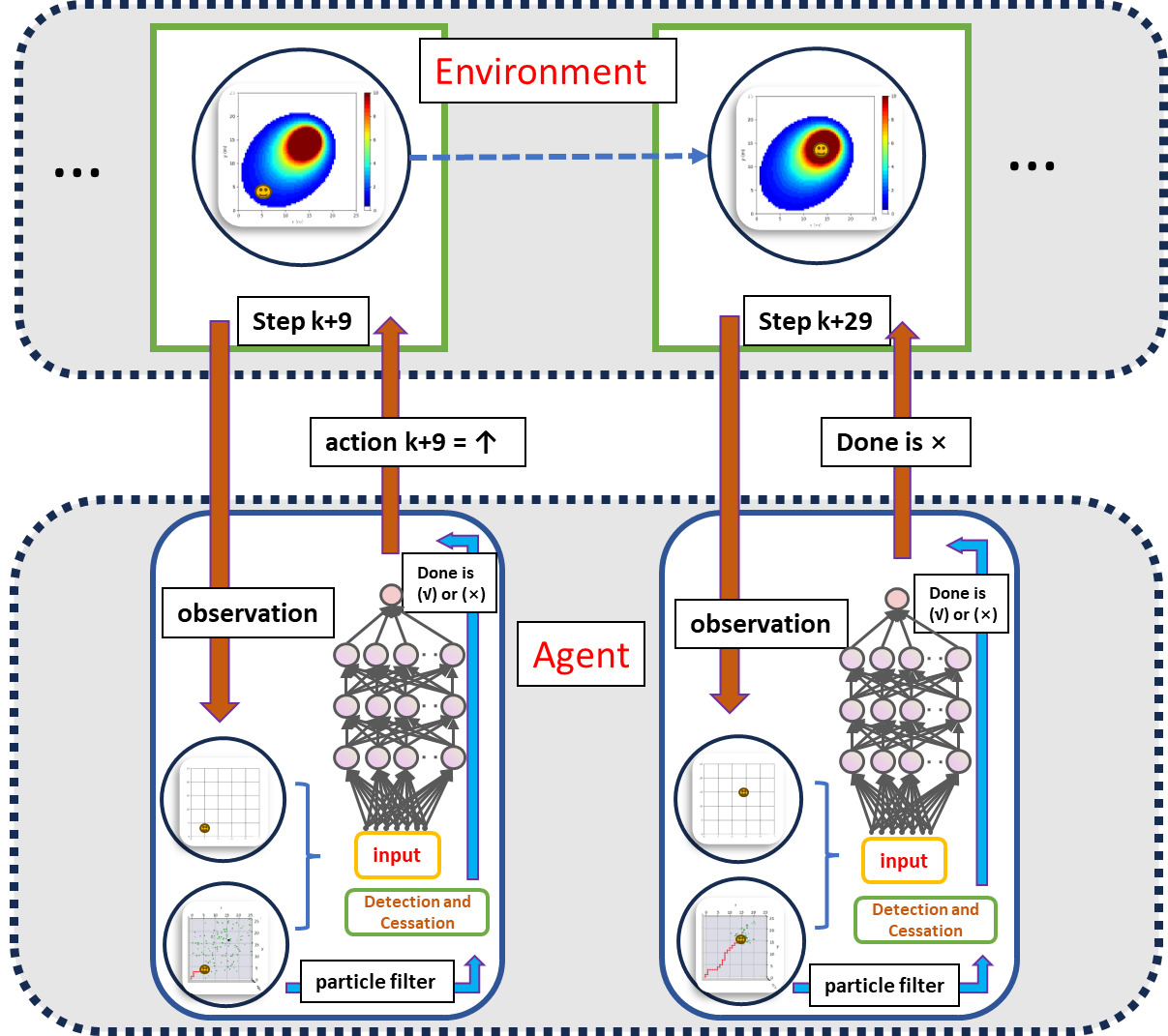
Figure 1: AGDC Structure Diagram for Solving the STE

Source Term Estimation involves identifying the location and characteristics (such as release rate) of hazardous gas emissions in the atmosphere, which is crucial for environmental monitoring and emergency response. However, this task presents several challenges. Firstly, the environment often does not provide clear cessation signals, and gas releases are typically invisible. Secondly, atmospheric turbulence results in sensor data that is sparse, intermittent, and time-varying. Additionally, direct measurements within the hazardous material dispersion area are often dangerous. Furthermore, sensor measurements are highly affected by noise and discontinuity. Consequently, agents must rapidly adjust their strategies in response to environmental changes and accurately estimate the source term despite unclear feedback. These challenges render source term estimation a complex task with significant uncertainty.

Statistical-based methods such as Infotaxis, Entrotaxis , and Dual Control for Exploitation and Exploration (DCEE) provide some solutions to these challenges. Infotaxis in [16, 17, 18] guides the search process by maximizing the rate of information acquisition, gradually reducing uncertainty to approximate the source of the gas. It is suitable for situations with high uncertainty regarding the gas source location but suffers from poor real-time performance and a tendency to get stuck in local optima. Entrotaxis in [19, 20] minimizes the entropy of future measurements to guide path selection, optimizing information acquisition based on real-time measurement data. It performs robustly in noisy environments but has poor adaptability in dynamic settings or sudden changes, making rapid adjustments difficult. DCEE in [21, 22] combines strategies of exploitation and exploration by dynamically adjusting the balance between the two, optimizing information acquisition and path selection. Suitable for highly variable environments, this strategy is complex to implement, requiring precise design of the trade-off mechanism between exploration and exploitation. Although these methods are effective in addressing the lack of environmental feedback and clear cessation signals, they share several common limitations: poor real-time performance, poor adaptability in rapidly changing environments, a tendency to get stuck in local optima, and complexity in implementation, particularly for the DCEE.

While Reinforcement Learning offers control capabilities, significantly improving efficiency and success rates, and avoiding local optima with good generalization capabilities, it effectively overcomes the limitations of statistical methods. However, RL struggles to effectively identify and autonomously cease goals in the absence of clear feedback. Traditional statistical methods consist of two modules: one for providing the agent with reward signals based on estimates, where rewards or information gain originate, and the other for determining the optimal action based on information gain. By replacing the control module of traditional statistical methods with RL while retaining the estimation module, a self-feedback mechanism can be introduced to RL. This helps RL algorithms check and cease goals at appropriate times. Although the rewards for the agent remain sparse in this context, the self-feedback mechanism provides signals from the agent itself rather than the environment, thus better supporting the training process.

Building on this foundation, we propose the concept of Autonomous Goal Detection and Cessation to address the STE problem using RL. AGDC introduces an autonomous goal detection and cessation mechanism within the RL framework, enabling the agent to automatically recognize and cease actions upon task completion. Specifically, the AGDC module employs Bayesian inference to estimate environmental dynamics and dynamically assess task progress. When the standard deviation of the estimated parameter values for environmental dynamics reaches a preset threshold, a cessation signal is automatically triggered. This approach not only addresses the issue of insufficient environmental feedback but also significantly enhances the adaptability and effectiveness of RL in complex and dynamic environments. By integrating the self-feedback mechanism with AGDC, RL algorithms can more efficiently accomplish STE tasks, thereby significantly improving capabilities in environmental monitoring and emergency response. The AGDC structure diagram is shown in Figure 1.

The main contributions of this paper are as follows: (1) We are the first to introduce, to the best of our knowledge, the AGDC module, which enables agents to autonomously recognize and evaluate goals, significantly increasing the capability of RL algorithms in feedback-limited environments. (2) We demonstrate the successful integration of AGDC with multiple RL algorithms in addressing the STE problem, achieving notable improvements over traditional methods. (3) Extensive experimental results confirm the superiority of AGDC-enhanced RL algorithms in terms of success rate, traveled distance, and search time, particularly in challenging environments with high uncertainty and limited feedback.

2 Problem Formulation and Peliminaries

In a two-dimensional search area denoted as $\Omega\subseteq\mathbb{R}^{2}$, where there is an expectation of encountering a hazardous release, a robot equipped with a gas sensor is tasked with traversing the area to calculate the release parameters, also referred to as the source term $\Theta_{s}$. This data will serve as the requisite input for a convection-diffusion model [16], enabling the generation of hazard forecasts. Within this context, in an environment characterized by average wind speed $u_{s}\in\mathbb{R}^{+}$ in meters per second (m/s), wind direction $\phi_{s}$ in radians (rad), and diffusivity $d_{s}$ in meters squared per second (m²/s), we detect the concentration of a hazardous substance $x_{k}\in\mathbb{R}^{+}$ using a robot or a sensor located at position $p_{k}=[x_{k},y_{k}]^{T}\in\Omega$ in meters (m). This hazardous material stems from a source term located at $p_{s}\in\Omega$, and it is released at a rate/strength $q_{s}\in\mathbb{R}^{+}$ in grams per second (g/s) with an average lifespan of $\tau_{s}\in\mathbb{R}^{+}$ in seconds (s).

Consequently, the parameters of the source term can be represented as follows:

$$\Theta_{s}=[p_{s}^{T},q_{s},u_{s},\phi_{s},d_{s},\tau_{s}]^{T}$$ (1)

Note: It is assumed in this study that all other parameters, except for the location of the leak source, can be obtained through direct measurement. Therefore, the primary objective is to successfully obtain the source term $p_{s}^{T}$, as it is the most important information about the source term.

2.1 Gaseous Diffusion Model

The average gas concentration [23], denoted as $m(p|\Theta_{s})$, for a given location of the mobile sensor at position $p_{k}$ over a time duration of $\tau_{s}$, can be computed utilizing the parameters of the source term $\Theta_{s}$ as follows:

$$m(p_{k}|\Theta_{s})=\frac{q_{s}}{4\pi d_{s}\|p_{k}-p_{s}\|}\exp\left[\frac{-\|p_{k}-p_{s}\|}{\lambda}+\psi\right],$$

where

$$\psi ={-(x_{k}-x_{s})u_{s}\cos\phi_{s}}/{2d_{s}}{-(y_{k}-y_{s})u_{s}\sin\phi_{s}}/{2d_{s}}$$

$$\lambda =\sqrt{{d_{s}\tau_{s}}/{[1+\left({u_{s}^{2}\tau_{s}}/{4d_{s}}\right)}]}.$$

2.2 Sensor Models

When mobile robots equipped with sensors conduct gas concentration detection in an environment, the measurement results are influenced by both internal and external factors. Internal factors include the sensitivity and calibration issues of the sensors, as well as the robot’s internal dynamics during movement, such as vibrations and posture changes. These factors can significantly impact gas concentration measurements. For example, the sensitivity of metal–oxide gas sensors [24, 25, 26] can vary with atmospheric contaminants, causing fluctuations in resistance and, consequently, the voltage readings. Furthermore, calibration issues, as discussed in the context of uncalibrated sensors, can lead to inaccuracies in the measured gas concentrations.

External factors encompass environmental variations in gas temperature, humidity, and pressure, all of which can affect measurement results. Wind turbulence, in particular, is a major contributor to noise in sensor readings. This is modeled using Gaussian distributions to describe the uncertainty in gas concentration measurements more accurately. For instance, the noise caused by wind turbulence is represented as $\nu_{\text{wind}}\sim\mathcal{N}(0,\sigma_{\text{wind}}^{2})$, where $\sigma_{\text{wind}}$ is a parameter that characterizes the instability of the wind conditions.

Specifically, the noise due to internal factors from the sensor is represented as $v_{\text{inter}}$. Therefore, the value of the gas concentration $c(p_{k}|\Theta)$ measured by the robot at position $p_{k}$ is:

$$c(p_{k}|\Theta)=m(p_{k}|\Theta)+v_{\text{inter}},$$

where $v_{\text{inter}}\sim\mathcal{N}(u,\sigma)$ and $v_{\text{inter}}$ follows a normal distribution $\mathcal{N}$ with mean $u$ and variance $\sigma$. This Gaussian noise model is widely used to emulate sensor measurements in simulations, accounting for both wind turbulence and sensor errors.

In a 25-meter by 25-meter area, as an illustrative example, the gaseous diffusion model can provide the gas concentration (GC) at each location. The robot samples the value obtained from the gas concentration model, as shown in Figure (2(a)), while also considering the presence of noise in the measured values at each location, depicted in Figure (2(b)). The source term parameters in the gas model are $q_{s}=5\,\text{g/s},u_{s}=2\,\text{m/s},\phi_{s}=45^{\circ},d_{s}=2\,\text{m}^{2}/\text{s},\tau_{s}=10\,\text{s}$.

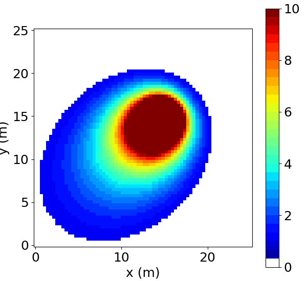
(a)

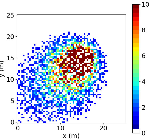
(b)

Figure 2: The example of map of the Gas-Diffusion model

In the STE problem, the robot can only obtain (or sample) the gas concentration measurements at its current location during the exploration process. Concentrations at other locations are not accessible, highlighting the importance of accurate sensor modeling and noise representation in ensuring reliable gas concentration measurements

2.3 Partially Observable Markov Decision Process

In the search area, the robot’s task is to estimate the location of a gas leak source with minimal movement steps. The robot lacks prior knowledge of the leak source’s location and gathers data through measurements at each step, making decisions based on this information. To address this challenge, we use the Partially Observable Markov Decision Process (POMDP) Reinforcement Learning method. This approach enables the robot to make effective decisions in an environment that is not fully observable, allowing for accurate localization of the gas leak source. A POMDP is a tuple $(S,O,A,T,Pr,R,\gamma)$, where $S$ is a set of states, $O$ is a set of observations, $A$ is a set of actions, $T(s^{\prime}|s,a):S\times A\rightarrow S$ is transition probabilities, $Pr(o|s,a):S\rightarrow O$ is observation probabilities, $R(s,a):S\times A\rightarrow\mathbb{R}$ is a reward function, and $\gamma$ is a discount factor. The objective in POMDP is to obtain an optimal policy to maximize expected cumulative rewards $\mathbb{E}{[\sum_{k=0}^{\infty}\gamma^{k}r_{k}]}$.

3 Methodology

3.1 Bayesian Approximation for Belief Distribution

The STE challenge is characterized as a Partially Observable Markov Decision Process, which implies that optimal decision-making cannot rely solely on the present observation, as complete state information in environment is not available. To address this issue, we have adopted this approach combining RL and Bayesian inference to effectively estimate environmental dynamics (belief) distribution and provide more unobservable information to assist decision-making.

Variational inference [27] and particle filter [28] are common Bayesian inference methods. The former approximates the target distribution by optimizing a differentiable lower bound but typically requires simplifying assumptions that may not suit complex environments. The latter, on the other hand, handles nonlinear and non-Gaussian distributions more effectively and adapts to dynamic conditions without needing such assumptions. Particle filter approximate the true distribution through sufficient sampling and offer flexibility in managing multimodal distributions, tracking potential source locations and release rates, and providing real-time updates. Therefore, particle filter outperform variational inference in STE problems.

The Particle filter is employed for iterative calculations of the environmental dynamics distribution. The belief distribution at time step $k$ is approximated using a set of $N$ particles, which are random samples $\{\Theta_{k}^{i},w_{k}^{i}\}_{i=1:N}$, where $\Theta_{k}^{i}$ represents the $i_{th}$ point estimation of source parameters (i.e., the belief), and $w_{k}^{i}$ is the associated weight, with $\sum_{i=1}^{N}w_{k}^{i}=1$. The approximated belief distribution $b(\Theta_{k})$ is expressed using samples and associated weights as follows:

$$b(\Theta_{k})=\sum_{i=1}^{N}w_{k}^{i}\delta(\Theta_{k}-\Theta_{k}^{i}),$$ (2)

where $\delta(\cdot)$ represents the Dirac delta function, which places all its weight at the value $\Theta_{k}^{i}$.

The sampling weights $\{w_{k}^{i}\}_{i=1:N}$ are updated through iterative sequential importance sampling [29]. At each step, a new sample of source parameter estimates $\{\Theta_{k}^{i}\}_{i=1:N}$ is obtained from the proposal distribution $q(\Theta_{k}^{i})$. Then, the unnormalized weight $\bar{w}_{k+1}^{(i)}$ corresponding to the source term vector $\Theta_{k}$ of the particle filter is updated as follows:

$$\bar{w}_{k+1}^{i} \propto w_{k}^{i}\cdot\frac{Pr(o_{k+1}|\Theta_{k+1}^{i})~{}T(\Theta_{k+1}^{i}|\Theta_{k}^{i})}{q(\Theta_{k+1}^{i}|\Theta_{k}^{i},{\bf o}_{1:k+1})}.$$ (3)

Obviously, although the dynamic environment and observation results may appear to change due to measurement errors and noise, the parameters constituting the environment (source term) remain fixed, leading to $\Theta_{k+1}=\Theta_{k}$ for $N$ particles. Assuming that the proposal distribution is consistent with the posterior distribution, the formula can be simplified as follows, (see additional materials for details):

$$\bar{w}_{k+1}^{i} =w_{k}^{i}\cdot Pr(o_{k+1}|\Theta_{k+1}^{i}).$$ (4)

Normalization of the sampling weights $w_{k}^{i}$ can be used to approximate the posterior distribution:

$$w_{k+1}^{i} =\frac{w_{k}^{i}\cdot Pr(o_{k+1}|\Theta_{k+1}^{i})}{\sum_{i=1}^{N}w_{k}^{i}\cdot Pr(o_{k+1}|\Theta_{k+1}^{i})}=\frac{\bar{w}_{k+1}^{i}}{\sum_{i=1}^{N}\bar{w}_{k+1}^{i}}.$$ (5)

As the number of learning iterations increases, the weights of most particles tend to zero, leading to the degeneracy problem. To address this issue, resampling is employed, and this method is based on the Markov Chain Monte Carlo move step [30].

We set a resampling threshold $\epsilon$, and when the number of effective samples falls below this threshold, the resampling process is triggered. The effective samples $N_{eff}$ are calculated by:

$$N_{eff}=\frac{1}{\sum_{i=1}^{N}(w_{k}^{i})^{2}}.$$ (6)

3.2 Autonomous Goal Detection and Cessation

Particle filter not only estimates the distribution of unknown environments but also combines with observational data to provide a more accurate representation of the true state. Additionally, it can generate self-cessation evaluation signals, indicating when computation can be ceased. When the goal is achieved, the particles forming the point estimate converge to a smaller range. By calculating the standard deviation of the particle parameters, the degree of parameter convergence can be observed, facilitating the judgment of goal completion progress.

1:  Initialize environment $\mathcal{E}$, policy $\pi$ and value function $V$, particle filter with $N$ particles

2:  for episode = 1 to $M$ do

3:     Initialize observation $o_{0}$ from $\mathcal{E}$, particles $\{\Theta\}_{i=1}^{N}$, state estimate $\hat{s}_{0}$ from particles $\{\Theta_{k}^{i}\}_{i=1}^{N}$ and observation $o_{0}$

4:     for  time step = 1 to $k$ do

5:        Sample $a_{k}\sim\pi_{\theta}(s_{k})$, $o_{k}\sim\mathcal{E}$

6:        Update particles $\{\Theta_{k}^{i}\}_{i=1}^{N}$ using particle filter

7:        for each particle $i$ do

8:           Sample new particle $\Theta_{k+1}^{i}\sim T(s_{k+1}|s_{k},a_{k})$

9:           Compute weight $w_{k+1}^{i}=w_{k}^{i}\cdot Pr(s_{k+1}|\Theta_{k+1}^{i})$

10:           if $N_{eff}<\epsilon$ then

11:              Normalize weights $w_{t}^{(i)}=\frac{w_{t}^{(i)}}{\sum_{j=1}^{N_{p}}w_{t}^{(j)}}$

12:              Resample $\{\Theta_{k+1}^{i}\}_{i=1}^{N}$ based on $\{w_{k+1}^{i}\}_{i=1}^{N}$

13:           end if

14:        end for

15:        $r_{k}\leftarrow$ 0, $done\leftarrow\text{False}$

16:        if $STD<\zeta$ then

17:           $r_{k}\leftarrow$ value$>0$, $done\leftarrow\text{True}$

18:        end if

19:        Estimate state $\hat{s}_{k+1}$ from $\{\Theta_{k}^{i}\}_{i=1}^{N}$ and $o_{k}$

20:        Update policy $\pi$ and $V$ using $\hat{s}_{k}$, $a_{k}$, $r_{k}$, and $\hat{s}_{k+1}$

21:        Set $o_{k}\leftarrow o_{k+1}$, $\hat{s}_{k}\leftarrow\hat{s}_{k+1}$

22:     end for

23:  end for

Algorithm 1 Reinforcement Learning with AGDC

When the standard deviation (STD) of the belief $\Theta_{k}$ by particle filter is lower than the given Cessation Threshold $\zeta$, the search ceases, and we consider the source term to be successfully estimated, meaning the goal is achieved. As a result, the agent rewards itself rather than relying on the environment. $STD$ is denoted as:

$$STD=\sqrt{diag(Cov(\Theta))},$$ (7)

where $Cov(\cdot)$ represents the covariance, and $diag(\cdot)$ denotes the trace of the matrix.

Calculating the STD of the particle filter belief and comparing it with a threshold as a signal to cease the search process is effective because the standard deviation reflects the concentration level of the belief distribution. A smaller standard deviation indicates that most particles are clustered around a certain estimate, suggesting that the belief state has converged. This convergence implies that the robot’s estimation of the source term parameters (such as the leak location) has become more accurate and stable. When the STD is less than the preset threshold $\zeta$, it indicates that the belief state estimation is sufficiently precise, making further algorithm execution yield diminishing returns, thus allowing the search process to cease, saving computational resources and time. Additionally, using the standard deviation as a cessation condition is relatively simple and intuitive, making it easier to implement and understand, facilitating easier decision-making and control in practical applications.

For example, suppose the covariance matrix of the particle filter belief state is:

$$Cov(\Theta)=\begin{pmatrix}\sigma_{x}^{2}&\sigma_{xy}\\ \sigma_{xy}&\sigma_{y}^{2}\end{pmatrix}$$

Using diag($\cdot)$, the standard deviations for the $x$ and $y$ coordinates can be calculated as:

$$STD_{x}=\sqrt{\sigma_{x}^{2}},\quad STD_{y}=\sqrt{\sigma_{y}^{2}}$$

This approach allows for an intuitive assessment of the uncertainty for each parameter. In contrast, directly calculating the standard deviation of the entire covariance matrix would require complex matrix operations, making the results less intuitive to understand. Therefore, using diag($\cdot$) for standard deviation calculation is a more effective and intuitive method. The details of the training algorithm are shown in Algorithm 1.

4 Experiment

In this paper, we utilized the STE Environment (STEenv) as the experimental platform to investigate the application of AGDC in RL. The STE Environment, described in Section 2 or [31] , comprises a Gaussian diffusion model and a sensor model. Instead of providing rewards to the Agent, it transmits the current position and the test concentration at that position as observations. Any RL algorithm can be integrated with the AGDC module to address the challenges posed by the STE problem.

4.1 Baseline Algorithms and Evaluation Metrics

There are three evaluation metrics in this paper: Success Rate (SR) to measure the number of successful source term estimations in the trajectories, Mean Traveled Distance (MTD) to represent the average distance traveled before a successful estimation occurs, and Search Time (ST) to measure the duration from the initiation of a search to the successful estimation of the target information. In this context, achieving a shorter traveled distance while successfully estimating the source’s location more frequently, along with a shorter search time indicating a quicker and more effective search process, signifies a more efficient approach.

We integrate the AGDC module into the DQN, PPO, and DDPG algorithms to address the STE problem. Additionally, we use four baseline approaches: Infotaxis, Entrotaxis, Dual Control for Exploitation and Exploration (DCEE), and a method that randomly selects actions for control. The first three are statistical methods, while the last one is a non-statistical method based on random action selection.

Infotaxis [16] aims to minimize the predicted posterior variance of the source location. It treats the search process as an information-gathering problem, where the objective is to reduce uncertainty about the source location.

Entrotaxis [19] enforces the maximum entropy sampling principle, which directs the agent to move towards positions of maximum uncertainty to gather more informative data about the environment and the source location.

DCEE [21] integrates both exploitation and exploration by incorporating the uncertainty into the control decisions, thus allowing the robot to not only move towards the estimated target but also probe the environment to reduce uncertainty.

Random involves selecting actions randomly, without any strategic guidance or optimization. It serves as a non-statistical baseline to compare against more sophisticated methods, highlighting the benefits of informed and strategic action selection.

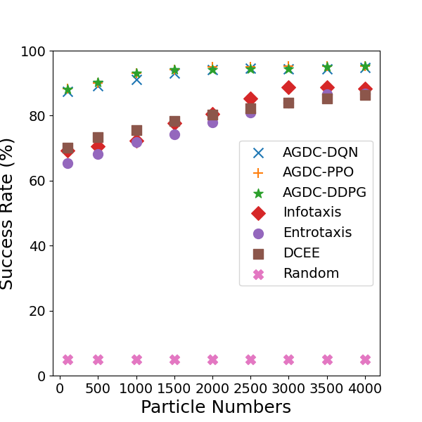
(a) Success Rates Across PN

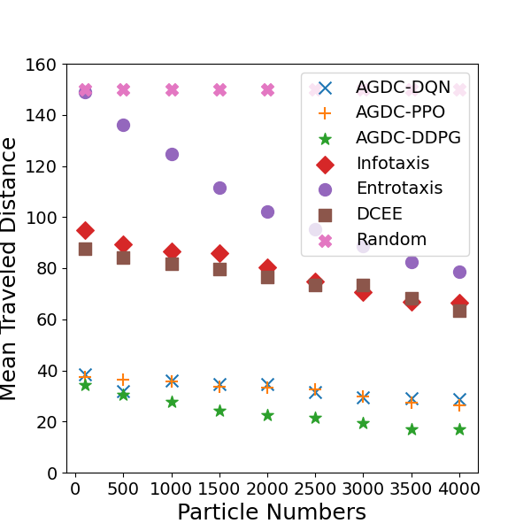
(b) Mean Traveled Distance Across PN

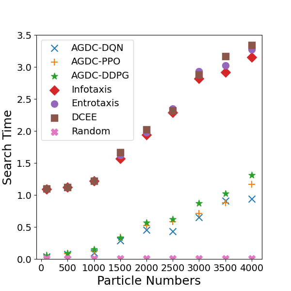
(c) Search Time Across PN

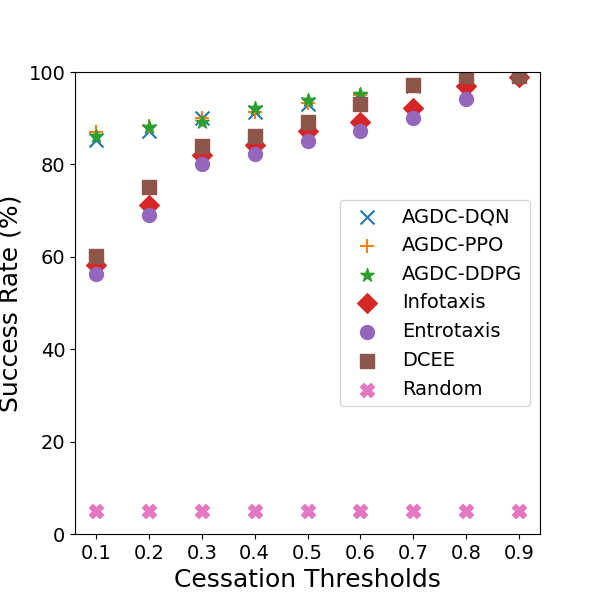
(d) Success Rates Across CT

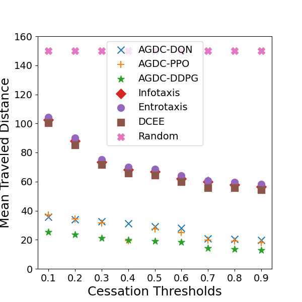
(e) Mean Traveled Distance Across CT

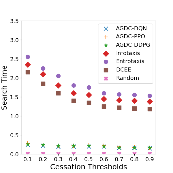
(f) Search Time Across CT

Figure 3: Comparative Analysis of Particle Numbers (PN) and Cessation Thresholds(CT)

Table 1: Parameter Distributions for the Training Scenarios

Source Parameter	Distribution
Source Location $x_{s}$	Uniform $\mathcal{U}(10,25)$
Source Location $y_{s}$	Uniform $\mathcal{U}(10,25)$
Release Strength $q_{s}$	Uniform $\mathcal{U}(100,500)$
Wind Speed $u_{s}$	Uniform $\mathcal{U}(1,4)$
Wind Direction $\phi_{s}$	Uniform $\mathcal{U}(0,360)$
Diffusivity $d$	Uniform $\mathcal{U}(1,8)$
Sensor Noise $\alpha$	Fixed at 0.3
Environmental Noise $\beta$	Fixed at 0.2
Effective Samples $N_{eff}$ $\beta$	Fixed at 0.5

4.2 Scenario Parameterization and Evaluation

The parameters for the training scenarios, set within a $30\times 30$ area, are constructed by randomly initializing the source and environmental properties at the beginning of each training episode, including parameters such as the gas source location, wind speed, and wind direction, all of which are sampled from the probability distributions presented in Table 1. The agent starts its search from a random location within the $(0,5)\times(0,5)$ area, with a speed of 1 meter per step, ensuring that it encounters a diverse set of scenarios during training, thereby promoting robust learning. The parameters for the testing scenarios consist of 1,000 randomly generated conditions that are not used during training. Although these scenarios are generated from the same parameter ranges as the training data, they present different specific conditions to ensure that the model is evaluated on unseen data.

4.3 Particle Numbers and Cessation Thresholds

We will discuss the effectiveness of integrating the AGDC module with RL by comparing three AGDC-enhanced RL algorithms against four baseline methods. Before delving into these comparisons, it is important to introduce two critical hyperparameters: Particle Numbers (PN) and Cessation Thresholds (CT) $\zeta$. The Particle Numbers are pivotal for AGDC as they determine the number of samples used to approximate the point distribution, which is essential for accurately estimating the belief necessary for goal detection. The Cessation Thresholds are directly linked to the cessation aspect of AGDC, as they define the criteria for deciding when to stop the task, ensuring that the process concludes at the most appropriate moment. Two groups of experiments were conducted to investigate the impact of two key hyperparameters on the performance of different algorithms. The first group analyzed the variations in success rate, mean traveled distance, and search time as the number of particles increased from 100 to 4000. The second group examined algorithm performance under different cessation thresholds, ranging from 0.1 to 0.9. The results are presented in Figure 3. The trajectories of six methods (excluding the random method) are shown in Figure 4.

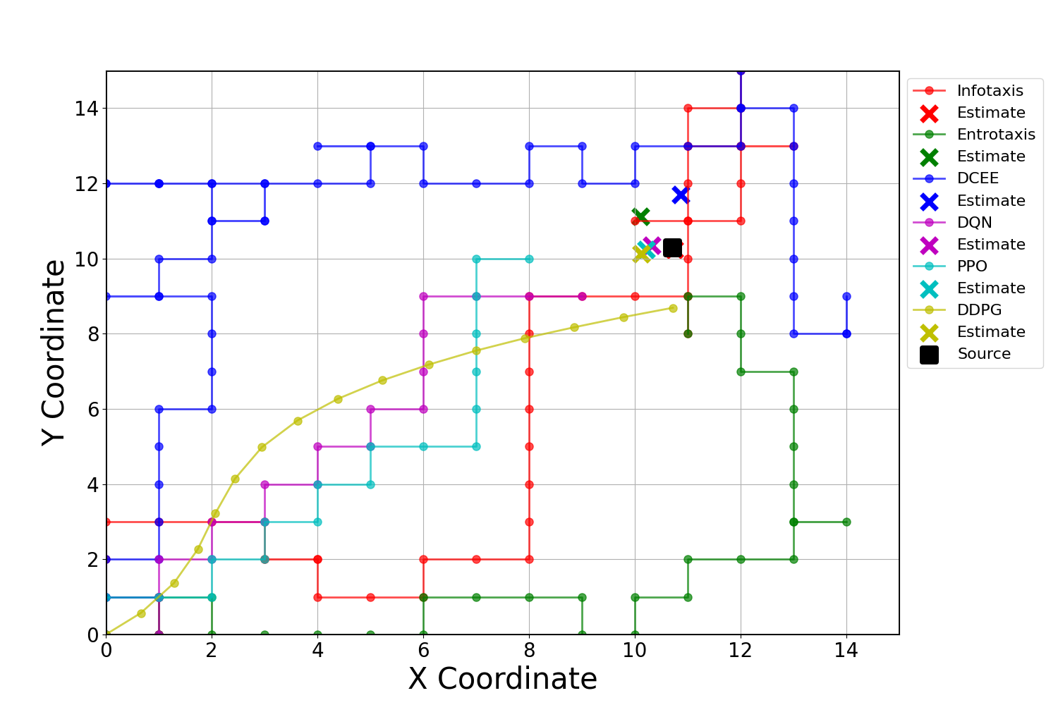
Figure 4: Trajectories of Various Methods

Analysis Across Various Particle Numbers: The success rates of AGDC-enhanced RL algorithms, such as AGDC-DQN, AGDC-PPO, and AGDC-DDPG, improve steadily with increasing particle numbers, reaching 95.27% for AGDC-PPO at 4000 particles. These algorithms outperform baseline methods like Infotaxis, Entrotaxis, and DCEE, which also benefit from more particles but remain less effective. The Random method remains largely ineffective, with success rates below 5%, regardless of particle count. Notably, DDPG’s continuous action space allows for more flexible movement compared to the discrete steps of other methods. AGDC-enhanced algorithms also show a consistent reduction in mean traveled distance as particle numbers increase. For instance, AGDC-DDPG reduces its mean distance from 34.33 at 100 particles to 16.83 at 4000, demonstrating greater efficiency. In contrast, baseline methods like Entrotaxis exhibit significantly higher distances, highlighting their inefficiency. The Random method, unaffected by particle count, continues to exhibit very high traveled distances. Regarding search time, AGDC-enhanced algorithms consistently achieve quicker convergence compared to baseline methods. AGDC-DQN, for example, maintains a search time of 0.94 units at 4000 particles. In contrast, methods like Infotaxis take significantly longer, reaching 3.15 units, indicating slower and less effective strategies. The Random method, despite its speed, fails to produce meaningful results, underscoring its overall inefficiency.

Figure 5: Multiple Trajectories from True Trajectory and Estimated (Belief) Trajectory with Color Gradient

Analysis Across Various Cessation Thresholds: The success rates of AGDC-enhanced algorithms, including AGDC-DQN, AGDC-PPO, and AGDC-DDPG, improve with higher cessation thresholds, with AGDC-PPO achieving 99.13% at a threshold of 0.9. This is due to the algorithms accumulating more confidence before stopping, leading to greater accuracy. Although Infotaxis and Entrotaxis also improve with higher thresholds, they require significantly more time and distance to reach similar success levels. As cessation thresholds rise, AGDC-enhanced algorithms also show reduced mean traveled distances, reflecting more efficient search cessation. AGDC-DDPG, for instance, reduces its distance to 12.8 units at a threshold of 0.9, while Infotaxis, even at its best, remains at 56.4 units, much higher than AGDC-DDPG. Search times for AGDC-enhanced algorithms decrease with higher thresholds, with AGDC-PPO reducing its time to 0.17 units at a threshold of 0.9. This indicates that these algorithms can efficiently conclude the search once confident in their estimation. However, excessively high thresholds may artificially inflate success rates and reduce traveled distances, creating a misleading appearance of improved performance by lowering the task’s rigor. Therefore, we advocate for setting an appropriate threshold that balances accuracy and task difficulty.

4.4 Further Research Experiments

An additional experiment was conducted to explore the AGDC module through a visualization approach. This experiment uses only the AGDC-based QDN method, with the environment set within a 20×20 area, and the source randomly located within the x, y from $\mathcal{U}(15,20)$. The experimental results are shown in Figure 5 and 6. In Figure 5, 100 trajectories are displayed, with the red lines representing the agent’s actual paths. The color intensity correlates with the time step count, with darker lines indicating more steps. The blue lines show the changes in the estimated source position. As the agent gets closer to the true source location (the goal), the estimated position (derived from Belief) also becomes more accurate, converging towards the goal.

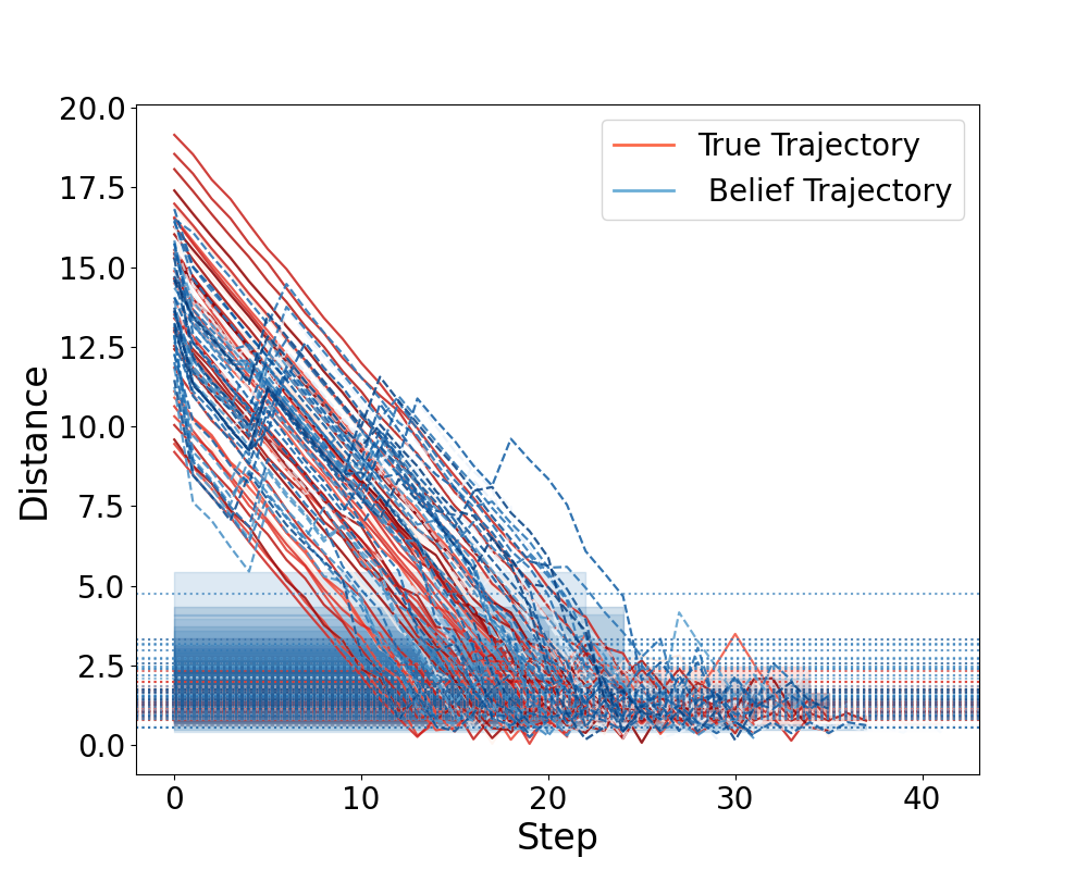
Figure 6: Distance from current position to goal and estimated belief at each step

Similarly, in Figure 6, the red line represents the distance between the agent and the true goal at each step, while the blue line shows the distance between the agent and the current estimated position. The red line in Figure 6 is relatively smooth, indicating that the agent consistently moves towards the true goal, even without knowing its exact location. This can explain why AGDC-based RL methods are efficient, as they avoid taking redundant steps. During this process, the estimated position (Belief) fluctuates with the incoming information but eventually converges near the true goal. We observed that towards the end, the blue line closely aligns with the red line, indicating high estimation accuracy. By setting different CT $\zeta$, represented by the horizontal blue lines, we can determine varying success rates based on the number of red line points below the threshold. This explains why a larger threshold increases the success rate; however, when set too high, the prediction becomes distorted. Combining insights from both figures, we conclude that the agent can effectively achieve Autonomous Goal Detection and Cessation in a gradual manner. Even though the red line may not be available in real-time, the trend of the blue line can still be used to roughly estimate the current progress of recognition, which serves as a form of explainability for ADGC.

5 Conclusion

In this study, we introduced the concept of Autonomous Goal Detection and Cessation within the Reinforcement Learning framework to address the challenges of STE. By integrating Bayesian inference with Reinforcement Learning, AGDC enhances the agent’s ability to autonomously detect and cease actions upon achieving the goal, significantly improving adaptability and efficiency in complex and dynamic environments. Our experiments demonstrate that AGDC-based methods consistently outperform traditional statistical approaches in terms of success rate, traveled distance, and search time across varying scenarios. This indicates that AGDC provides a robust mechanism for agents to effectively navigate uncertain environments, making it a valuable tool for applications in environmental monitoring and emergency response. Future work could explore the scalability of AGDC to more complex multi-agent systems and real-world deployment scenarios.

References

- [1] V. Mnih, K. Kavukcuoglu, D. Silver, A. A. Rusu, J. Veness, M. G. Bellemare, A. Graves, M. Riedmiller, A. K. Fidjeland, G. Ostrovski et al., “Human-level control through deep reinforcement learning,” nature, vol. 518, no. 7540, pp. 529–533, 2015.
- [2] D. Silver, J. Schrittwieser, K. Simonyan, I. Antonoglou, A. Huang, A. Guez, T. Hubert, L. Baker, M. Lai, A. Bolton et al., “Mastering the game of go without human knowledge,” nature, vol. 550, no. 7676, pp. 354–359, 2017.
- [3] X. Wang, S. Zhang, W. Zhang, W. Dong, J. Chen, Y. Wen, and W. Zhang, “Zsc-eval: An evaluation toolkit and benchmark for multi-agent zero-shot coordination,” arXiv preprint arXiv:2310.05208, 2024.
- [4] X. Wang, Z. Zhang, and W. Zhang, “Model-based multi-agent reinforcement learning: Recent progress and prospects,” arXiv preprint arXiv:2203.10603, 2022.
- [5] S. Levine, C. Finn, T. Darrell, and P. Abbeel, “End-to-end training of deep visuomotor policies,” Journal of Machine Learning Research, vol. 17, no. 39, pp. 1–40, 2016.
- [6] W. Zhang, X. Wang, J. Shen, and M. Zhou, “Model-based multi-agent policy optimization with adaptive opponent-wise rollouts,” arXiv preprint arXiv:2105.03363, 2021.
- [7] X. Wang, Z. Tian, Z. Wan, Y. Wen, J. Wang, and W. Zhang, “Order matters: Agent-by-agent policy optimization,” in The Eleventh International Conference on Learning Representations.
- [8] S. Feng, H. Sun, X. Yan, H. Zhu, Z. Zou, S. Shen, and H. X. Liu, “Dense reinforcement learning for safety validation of autonomous vehicles,” Nature, vol. 615, no. 7953, pp. 620–627, 2023.
- [9] B. R. Kiran, I. Sobh, V. Talpaert, P. Mannion, A. A. Al Sallab, S. Yogamani, and P. Pérez, “Deep reinforcement learning for autonomous driving: A survey,” IEEE Transactions on Intelligent Transportation Systems, vol. 23, no. 6, pp. 4909–4926, 2021.
- [10] J. Degrave, F. Felici, J. Buchli, M. Neunert, B. Tracey, F. Carpanese, T. Ewalds, R. Hafner, A. Abdolmaleki, D. de Las Casas et al., “Magnetic control of tokamak plasmas through deep reinforcement learning,” Nature, vol. 602, no. 7897, pp. 414–419, 2022.
- [11] R. Meyes, H. Tercan, S. Roggendorf, T. Thiele, C. Büscher, M. Obdenbusch, C. Brecher, S. Jeschke, and T. Meisen, “Motion planning for industrial robots using reinforcement learning,” Procedia CIRP, vol. 63, pp. 107–112, 2017.
- [12] Y. Li, S. Zhang, J. Sun, Y. Du, Y. Wen, X. Wang, and W. Pan, “Cooperative open-ended learning framework for zero-shot coordination,” in International Conference on Machine Learning. PMLR, 2023, pp. 20 470–20 484.
- [13] Y. Li, S. Zhang, J. Sun, W. Zhang, Y. Du, Y. Wen, X. Wang, and W. Pan, “Tackling cooperative incompatibility for zero-shot human-ai coordination,” Journal of Artificial Intelligence Research, vol. 80, pp. 1139–1185, 2024.
- [14] Z. Xu, H. Mao, N. Zhang, X. Xin, P. Ren, D. Li, B. Zhang, G. Fan, Z. Chen, C. Wang et al., “Beyond local views: Global state inference with diffusion models for cooperative multi-agent reinforcement learning,” arXiv preprint arXiv:2408.09501, 2024.
- [15] H. Steiner and W. Bushe, “Large eddy simulation of a turbulent reacting jet with conditional source-term estimation,” Physics of Fluids, vol. 13, no. 3, pp. 754–769, 2001.
- [16] M. Vergassola, E. Villermaux, and B. I. Shraiman, “‘infotaxis’ as a strategy for searching without gradients,” Nature, vol. 445, no. 7126, pp. 406–409, 2007.
- [17] M. Hutchinson, C. Liu, and W.-H. Chen, “Information-based search for an atmospheric release using a mobile robot: Algorithm and experiments,” IEEE Transactions on Control Systems Technology, vol. 27, no. 6, pp. 2388–2402, 2018.
- [18] A. Loisy and C. Eloy, “Searching for a source without gradients: how good is infotaxis and how to beat it,” Proceedings of the Royal Society A, vol. 478, no. 2262, p. 20220118, 2022.
- [19] M. Hutchinson, H. Oh, and W.-H. Chen, “Entrotaxis as a strategy for autonomous search and source reconstruction in turbulent conditions,” Information Fusion, vol. 42, pp. 179–189, 2018.
- [20] Y. Zhao, B. Chen, Z. Zhu, F. Chen, Y. Wang, and D. Ma, “Entrotaxis-jump as a hybrid search algorithm for seeking an unknown emission source in a large-scale area with road network constraint,” Expert Systems with Applications, vol. 157, p. 113484, 2020.
- [21] W.-H. Chen, C. Rhodes, and C. Liu, “Dual control for exploitation and exploration (dcee) in autonomous search,” Automatica, vol. 133, p. 109851, 2021.
- [22] C. Rhodes, C. Liu, and W.-H. Chen, “Autonomous source term estimation in unknown environments: From a dual control concept to uav deployment,” IEEE Robotics and Automation Letters, vol. 7, no. 2, pp. 2274–2281, 2022.
- [23] Y. Zhao, B. Chen, X. Wang, Z. Zhu, Y. Wang, G. Cheng, R. Wang, R. Wang, M. He, and Y. Liu, “A deep reinforcement learning based searching method for source localization,” Information Sciences, vol. 588, pp. 67–81, 2022.
- [24] J.-G. Li, Q.-H. Meng, Y. Wang, and M. Zeng, “Odor source localization using a mobile robot in outdoor airflow environments with a particle filter algorithm,” Autonomous Robots, vol. 30, pp. 281–292, 2011.
- [25] P. P. Neumann, V. Hernandez Bennetts, A. J. Lilienthal, M. Bartholmai, and J. H. Schiller, “Gas source localization with a micro-drone using bio-inspired and particle filter-based algorithms,” Advanced Robotics, vol. 27, no. 9, pp. 725–738, 2013.
- [26] P. P. Neumann and M. Bartholmai, “Real-time wind estimation on a micro unmanned aerial vehicle using its inertial measurement unit,” Sensors and Actuators A: Physical, vol. 235, pp. 300–310, 2015.
- [27] M. I. Jordan, Z. Ghahramani, T. S. Jaakkola, and L. K. Saul, “An introduction to variational methods for graphical models,” Machine learning, vol. 37, pp. 183–233, 1999.
- [28] N. J. Gordon, D. J. Salmond, and A. F. Smith, “Novel approach to nonlinear/non-gaussian bayesian state estimation,” in IEE proceedings F (radar and signal processing), vol. 140, no. 2. IET, 1993, pp. 107–113.
- [29] S. T. Tokdar and R. E. Kass, “Importance sampling: a review,” Wiley Interdisciplinary Reviews: Computational Statistics, vol. 2, no. 1, pp. 54–60, 2010.
- [30] B. Ristic, S. Arulampalam, and N. J. Gordon, “Beyond the kalman filter: Particle filters for tracking applications,” 2004. [Online]. Available: https://api.semanticscholar.org/CorpusID:60500010
- [31] Y. Shi, K. McAreavey, C. Liu, and W. Liu, “Reinforcement learning for source location estimation: A multi-step approach,” in 2024 IEEE International Conference on Industrial Technology (ICIT), 2024, pp. 1–8.