Using Synthetic Data to Mitigate Unfairness and Preserve Privacy through Single-Shot Federated Learning
Abstract
To address unfairness issues in federated learning (FL), contemporary approaches typically use frequent model parameter updates and transmissions between the clients and server. In such a process, client-specific information (e.g., local dataset size or data-related fairness metrics) must be sent to the server to compute, e.g., aggregation weights. All of this results in high transmission costs and the potential leakage of client information. As an alternative, we propose a strategy that promotes fair predictions across clients without the need to pass information between the clients and server iteratively and prevents client data leakage. For each client, we first use their local dataset to obtain a synthetic dataset by solving a bilevel optimization problem that addresses unfairness concerns during the learning process. We then pass each client’s synthetic dataset to the server, the collection of which is used to train the server model using conventional machine learning techniques (that do not take fairness metrics into account). Thus, we eliminate the need to handle fairness-specific aggregation weights while preserving client privacy. Our approach requires only a single communication between the clients and the server, thus making it computationally cost-effective, able to maintain privacy, and able to ensuring fairness. We present empirical evidence to demonstrate the advantages of our approach. The results illustrate that our method effectively uses synthetic data as a means to mitigate unfairness and preserve client privacy.
1 Introduction
Fairness and privacy have become increasingly visible concerns as more machine learning (ML) tools are deployed in the real world. In the pursuit of highly accurate ML models, one often observes discriminatory outcomes when the training is performed using unfair/biased data. Discrimination here refers to decisions made against certain groups based on a sensitive feature, such as race, age, or gender (Mehrabi et al. 2021). For example, racial bias has been identified in the commercial risk assessment tool COMPAS (Dressel and Farid 2018) and in health systems (Obermeyer et al. 2019). Commercial facial recognition technologies have shown accuracy disparities by gender and skin type (Buolamwini and Gebru 2018). Additionally, age-related bias has been found in facial emotion detection systems (Kim et al. 2021). To mitigate such discriminatory practices, a collection of pre-processing, in-processing, and post-processing techniques have been studied in a data-centralized setting (Mehrabi et al. 2021; Caton and Haas 2024; Wang, Shu, and Culotta 2021; Zafar et al. 2017; Lohia et al. 2019; d’Alessandro, O’Neil, and LaGatta 2017). These rely on access to the entire dataset, which in turn raises privacy leakage concerns. Thus, they are not applicable to decentralized data environments such as in the context of Federated Learning (FL).
FL has emerged as a promising paradigm that prioritizes data privacy. FL involves training client models using local data, sending the resulting client models to a server, then learning a server model by aggregating the client models using an iterative process, thereby avoiding the need to have direct access to client data (McMahan et al. 2017). Since the server model is indirectly derived from client data by using the client models as intermediaries, it is expected to lead to good representation and generalization across all clients (Pan et al. 2023). Separate from the typical distributed optimization setting, there are challenges in addressing fairness concerns in FL that include non-IID or unbalanced client datasets, massively distributed clients, and limited communication capacity between the clients and server (McMahan et al. 2017). If some client datasets are inherently unfair, perhaps reflecting demographic or regional disparities, then this can lead to unfair server models after aggregation steps are performed. Ensuring fairness across multiple independent client models is difficult in this situation.
When considering fairness in FL, prior studies have primarily focused on using aggregation to obtain a fair server model. However, these methods usually require frequent transmission of model-related information between clients and the server, which leads to significant communication costs. Furthermore, additional client information, such as dataset size or unfairness measures, is needed to calculate the server model aggregation weights, which in turn leads to potential information leakage. Addressing these limitations is critical for advancing fairness in the FL context.
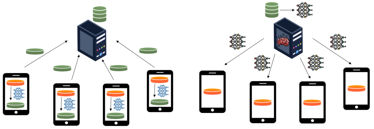
To mitigate the aforementioned drawbacks, we propose an approach that only transfers synthetic client datasets to the server instead of client models. The framework is illustrated in Figure 1. Each synthetic client dataset is learned from the client’s own training data with fairness considerations incorporated into the training process by solving a bilevel optimization problem. The server model is then trained on a combined (synthetic) dataset to minimize loss, just like training a typical data-centralized machine learning model without explicit fairness concerns. Since the client training data is preserved on the client devices and no additional information needs to be sent to the server for calculating model aggregation weights, this approach prevents any client information leakage. Moreover, this approach is designed as a one-time model transmission between the clients and server. Once the server model is trained, the entire algorithm is completed when the server model is passed back to the clients. This greatly reduces transmission costs.
We summarize our contributions as follows:
-
•
To the best of our knowledge, this is the first FL approach that involves only a single transmission between the clients and server while also addressing unfairness issues. Thus, our approach avoids high transmission costs while still producing a fair server model.
-
•
Our approach prevents potential client information leakage by involving only a single transmission of synthetic data from each client to the server. Our experiments show that an accurate, but also fair server model can be trained even though the synthetic client data can differ significantly from the original client data.
-
•
A major advantage of our approach is that the server model can be trained without fairness concerns. In a sense, the synthetic client data has already been generated to take fairness concerns into account, so all the server needs to do is aggregate the client data and train to maximize prediction accuracy.
-
•
We validate our approach empirically on datasets from the literature. We provide concrete numerical evidence that our approach results in highly accurate and fair ML models without leaking private client information.
2 Background and Related Work
In this section, we discuss background and related work on group fairness measures, fairness in federated learning, bilevel optimization, and synthetic data generation.
Group Fairness Measures
In ML and FL, group fairness is a commonly used metric for determining whether a common group of people—as determined by a “sensitive feature” (e.g., gender, race, or age)—is treated fairly. One of the prominent group fairness measures is statistical parity (SP), also known in this context as demographic parity. SP defines fairness as the equal probability of predicting positive labels for different sensitive groups, i.e., for groups characterized by the value of a sensitive feature.
To define SP concretely, let (resp., ) be a random vector representing nonsensitive (resp., sensitive) features and let be a binary-valued random variable representing a label, all defined over a combined probability space with probability measure . For convenience, let . Let denote a binary classification function defined with weights . Then, as used in Caton and Haas (2024), the binary classifier is said to have SP if and only if
| (1) |
From a computational perspective, enforcing equation (1) is challenging because the probabilities lead to nonconvex functions. Zafar et al. (2019) used the decision boundary covariance as an approximation of the group conditional probabilities. In particular, the decision boundary covariance is defined as the covariance between the sensitive feature and the signed distance between the features and the decision boundary. Thus, letting denote this distance function corresponding to , the decision boundary covariance is
| (2) | ||||
where (Zafar et al. 2017), is a sample of , and is the average of .
In this study, we use a linear predictor, i.e., . Using this choice, and keeping in mind our goal to obtain fair predictive models in terms of SP, we will present an optimization framework that enforces the constraint
| (3) |
where is a user-defined threshold that determines the level of unfairness that is to be tolerated. To evaluate the classifier in terms of SP, it is common to use the difference , which motivates the definition of the following measure of statistical parity difference defined over :
| (4) | |||
The closer SPD is to zero, the closer the predictor is to achieving perfect group fairness with respect to SP.
Fairness in Federated Learning
Proposed by McMahan et al. (2017), FL is a distributed optimization framework designed to address challenges related to data privacy and large-scale datasets. Given client objective functions , the standard FL objective function is
| (5) |
with being the number of clients. This formulation aims to minimize the average () of the local client objectives (), where is the model parameters (Pan et al. 2023). It is typical in ML that the client’s objective function has the form for some loss function .
Many FL algorithms work by having the clients produce parameter values , which are then passed to the server to obtain an estimate of a solution to (5). For example, the foundational FL algorithm FedAvg computes the server model update using the following aggregation formula:
| (6) |
where is the number of data points for client for each index and (McMahan et al. 2017).
Some previous studies have focused on how to aggregate the model parameters in a manner that may be able to obtain a fair server model. For example, FairFed computes each client’s aggregation weight as the difference in a fairness performance metric between the client model and the server model (Ezzeldin et al. 2023); FAIR-FATE incorporates momentum updates in the server model to prioritize clients with higher client fairness performance than the server model (Salazar et al. 2023); and FedGAN and Bias-Free FedGAN generate metadata from client generators on the server to ensure that a balanced training dataset is input to the server model (Rasouli, Sun, and Rajagopal 2020; Mugunthan et al. 2021). However, these algorithms rely on frequent communication of the model parameter values between the clients and the server. If client devices are slow or offline, the communication costs can be expensive and pose a significant limitation. Furthermore, in addition to the clients’ model parameters, extra client information such as dataset size and the fairness measures on local models must be passed to the server to compute the aggregation weights, which can lead to potential leakage of client statistics (Ezzeldin et al. 2023).
Bilevel Optimization
Bilevel optimization is characterized by the nesting of one optimization problem within the other. One formulation of a bilevel optimization problem can be written as follows:
| (7) | ||||
where and are the upper-level (or outer problem) and lower-level (or inner problem) objective functions, respectively. Note that allowable values for the upper-level problem variables is implicitly defined by the lower-level problem (Savard and Gauvin 1994; Giovannelli, Kent, and Vicente 2024). Due to the hierarchical structure, decisions made by the upper-level problem affect the outcomes of the lower-level problem (Sinha, Malo, and Deb 2017).
In this paper, we address fairness issues by formulating a bilevel optimization problem over clients. Our inner problem objective is to train a model with minimum loss from a given synthetic dataset. Our outer problem objective is to generate a synthetic dataset (one for each client) as the input to the inner problem. Moreover, when utilizing the model obtained from the inner problem and evaluating it on client training data, certain fairness constraints are enforced. The details of our approach are presented in the next section.
Synthetic Data Generation
Our approach is inspired by data distillation, which was first introduced in 2018 (Wang et al. 2018). Wang et al. (2018) presented the concept of distilling knowledge from a large training dataset into a small synthetic dataset. The idea is that the model trained on the synthetic dataset can perform approximately as well as one trained on the original large dataset. This method makes the training process more efficient and reduces the computational cost of model updates.
Synthetic data can also lead to benefits in the FL setting. In FL, the cost of communicating model parameter values between the server and clients is a major concern, especially when the model structure is complex and the number of model parameters is large. Goetz and Tewari (2020) and Hu et al. (2022) proposed transferring synthetic datasets to the server instead of the entire client model from the client side to reduce communication costs. The use of synthetic datasets helps in recovering the model update on the server to improve the server model updates (Goetz and Tewari 2020) or in recovering the client model directly to make server model aggregation more efficient (Hu et al. 2022).
The main contribution of these prior works is to make the training process efficient. They do not address fairness concerns. By contrast, we propose an extension of the previous works to improve fairness across clients in FL. While learning synthetic data for the clients, we not only distill the knowledge of their training data into the synthetic data but also mitigate unfairness in the training data at the same time. Consequently, when the model is trained by the server using the synthetic data from the clients, certain fairness criteria can be satisfied when the model is evaluated on the client’s original training data. In addition, we can fully control the synthetic dataset size and the composition of each sensitive group and label. Thus, when the synthetic data is sent to the server, we can help prevent client information leakage.
3 Proposed Approach
In this section, we introduce our framework, which consists of two main parts: training synthetic datasets on the client side, then training a global model on the server. For simplicity, we focus on the case with a single sensitive feature (denoted in ) and binary classification, although our approach could be generalized to other settings as well.
On the Client Side
We address fairness concerns on the client side through the use of SP as our fairness measure and the covariance decision boundary as a relaxation. Each client learns a synthetic dataset by solving the bilevel optimization problem in (8), stated below, which we now proceed to motivate.
Consider an arbitrary client. Assuming the client has data points, for each , we let be the th nonsensitive feature vector, be the th sensitive feature value, be the label of the th data point, be the complete th feature vector, and be the complete th data point. The goal of each client is to learn a synthetic dataset of size . To denote the synthetic dataset, for each , we let where , , , and .
Multiple strategies can be used to define . For example, if , then one can simply choose , whereas if once can choose the values for so that they have the same proportions as those for . Details on how we choose these values for our numerical experiments are provided in Section 4.
Once has been chosen, the “ideal” problem solved by the client is defined, for user-defined tolerances and loss function , as follows:
| (8) | ||||
where we define
The loss function can be chosen based on the task being performed. In this paper, since we focus on binary classification, we select the logistic loss function, which defined over has the following form:
| (9) |
where represents the model parameters.
The aim of problem (8) is to learn synthetic nonsensitive features in the synthetic dataset . The lower-level problem (or inner problem) is an unconstrained optimization problem that trains a model by minimizing the loss over the synthetic dataset. The upper-level problem (or outer problem) aims to minimize the loss of the model from the inner problem by evaluating it on the client’s actual training dataset while satisfying fairness constraints.
Regarding the fairness constraints in (8), we want the covariance between the predictions and the sensitive features in the client training data and the synthetic data to fall within certain thresholds (i.e., and ). In this way, it keeps SPD close to zero to achieve good group fairness. The fairness constraints can be changed for other purposes as needed, for example, to achieve equal opportunity (Mehrabi et al. 2021).
On the Server Side
After each client learns its synthetic dataset, it is passed to the server. The server then trains a model on the combined synthetic dataset (i.e., the collection of synthetic datasets passed to it by the clients) defined using the same modeling formulation as in the client’s inner optimization problem. Specifically, if we let denote the th data point for the th client, then the server computes the model parameters for the global model by solving the following problem:
| (10) |
We stress that the server solves a standard ML problem to learn its model parameters, i.e., it does not make any attempt to account for fairness. The fact that it might “automatically” compute a fair model is a direct consequence of how each client computes its synthetic dataset in our framework.
Complete Algorithm
Instead of choosing nonnegative parameters and , then solving the constrained optimization problem in (8), we choose to solve a penalty reformulation of (8) that takes the form of an unconstrained optimization problem, for the purposes of computational efficiency and convenience. Essentially, our penalty problem described below computes a solution to (8) for implicitly defined values of and .
For a given choice of penalty parameters , regularization parameters , and previously computed values for , we define
with
| (11) |
The penalty reformulation of (8) that we solve is given by
| (12) |
In this formulation, and are the penalty parameters associated with fairness constraints on the client’s original training data and synthetic data, respectively. Additionally, and are regularization parameters for the outer and inner problem, respectively. Regularization terms are frequently adopted in ML modeling formulations for a variety of reasons. The regularization used on the nonsensitive features in the outer problem help prevent the computation of excessively large values for , whereas the regularization term in the inner problem is introduced primarily to guarantee that the inner problem has a unique minimizer.
When required to solve the inner optimization problem (i.e., problem (11)), any solver designed for unconstrained optimization is applicable. In our testing, we choose the L-BFGS method with a strong Wolfe line search procedure.
To solve the outer optimization problem (12), we use a descent-type algorithm. Computing the gradient is nontrivial because of the inner optimization problem. That said, the gradient can be computed using the chain rule. Observe that
| (13) |
where has th row . Then, . Computing in (13) is straightforward while computing requires implicit differentiation to obtain
| (14) |
which amounts to solving a linear system of equations.
With respect to the training performed on the server, we also include a regularization term to be consistent with the inner subproblem (11). Specifically, by letting denote the th synthetic data point computed by client so that denotes the combined synthetic dataset from all clients, the server model parameters are trained by solving
| (15) |
The entire algorithm is shown in Algorithm 1. Client training starts at line 1, and server training begins at line 18. Unlike other conventional FL algorithms, which frequently communicate model parameters back and forth between the server and clients, our approach communicates parameter values in each direction a single time. Therefore, the transmission cost of our approach can be significantly less.
4 Experiments
In this section, we test through numerical experiments the performance of our approach. In particular, we examine how the penalty parameters and the size of the synthetic data affect the trade-off between accuracy and fairness metrics.
| Dataset | Law School | Dutch |
|---|---|---|
| Sensitive feature | race and gender | gender |
| Number of clients | 2 | 4 |
| 20798 | 60420 | |
| 8319 | 12084 | |
| 800 | 1200 | |
| 2080 | 3021 |

| Dataset | Law School (race) | Law School (gender) | Dutch (gender) | ||||
|---|---|---|---|---|---|---|---|
| Accuracy(%) | SPD | Accuracy(%) | SPD | Accuracy(%) | SPD | ||
| 0 | 88.44 | 0.4566 | 87.04 | 0.1320 | 78.21 | 0.2098 | |
| 10 | 87.91 | 0.0900 | 85.87 | 0.0150 | 76.85 | 0.0599 | |
| 100 | 86.20 | 0.0490 | 81.01 | 0.0151 | 76.56 | 0.0365 | |
| 1000 | 85.26 | 0.0400 | 73.89 | 0.0218 | 76.50 | 0.0344 | |
| 10000 | 85.22 | 0.0449 | 72.14 | 0.0224 | 74.33 | 0.0382 | |
| 0 | 88.51 | 0.4362 | 87.24 | 0.1233 | 78.25 | 0.2103 | |
| 10 | 87.86 | 0.0816 | 85.50 | 0.0010 | 76.67 | 0.0478 | |
| 100 | 86.23 | 0.0547 | 78.17 | -0.0014 | 76.62 | 0.0378 | |
| 1000 | 85.58 | 0.0375 | 77.74 | -0.0032 | 76.70 | 0.0390 | |
| 10000 | 84.30 | 0.0412 | 73.37 | 0.0080 | 76.23 | 0.0496 | |
Experimental Setup
Computing environment. The experiments reported in this paper were conducted on a machine equipped with an AMD Ryzen 9 7900X3D 12-Core CPU Processor. The FL framework was simulated using client parallel training implemented via the Python package multiprocessing.
Datasets. We present experiments for our approach on the binary classification datasets Law School (Wightman 1998) and Dutch (Van der Laan 2001), both of which are widely used real-world datasets used in the fairness-aware literature (Salazar et al. 2023). The Law School dataset consists of 11 features, including race and gender, which we treat as sensitive features in separate experiments. The goal is to predict whether a student will pass the bar exam. The Dutch dataset also has 11 features with gender identified as the sensitive feature. The task is to predict whether an individual’s occupation is prestigious. Additional details on how we partition the datasets for our tests are provided in Table 1. We remark that our tests use a relatively small number of clients since they are for demonstration purposes only, although we do expect that our results representative real-world settings as well (i.e., when ).
Hyperparameters and algorithm choices. We set the regularization parameter . The maximum number of L-BFGS iterations used when solving the inner problem (11) is , and in Algorithm 1. The iterate update in Line 14 of Algorithm 1 is performed using Adam (Kingma 2014). The penalty parameters and , regularization parameter , and synthetic dataset size of each client are discussed during each test that we present next.
Experimental Results
Ability to Mitigate Unfairness. To assess the ability of our method to mitigate unfairness, we first examine the trade-off between the accuracy lost and fairness gained by choosing different values for the penalty parameters and . These parameters correspond to the fairness constraints associated with the client’s original training data and synthetic data, respectively. For each client, we set and so that we may clearly observe whether the synthetic datasets have the ability to mitigate unfairness. We conduct our tests on the Law School dataset, where race is the sensitive feature, with . The results are depicted in Figure 2. The values are computed across all clients’ testing data.
One can view the bottom-left block in Figure 2 as a baseline since it corresponds to , i.e., no penalization on unfairness is enforced. Observing these metrics horizontally from left to right, we can see that the accuracy generally decreases, while the covariance and SPD measures approach zero thus reflecting a decrease in unfairness, although the trend is not perfectly monotone. Moreover, our results indicate that choosing leads to results that are significantly less predictable and robust. Finally, based on these results, one might be tempted to choose and , which leads to a mere drop in accuracy and a significant improvement in the fairness measures.
In Figure 2, we can observe for the choice of and that the accuracy was significantly lower than the other settings. For experimental purposes, for this setting we computed the same quantities after adjusting from to , which then achieved an accuracy of , a covariance of 0.056, and an SPD of . This further underscores the diminished robustness of our approach in the case when . In conclusion, we recommend using the value and tuning appropriately.
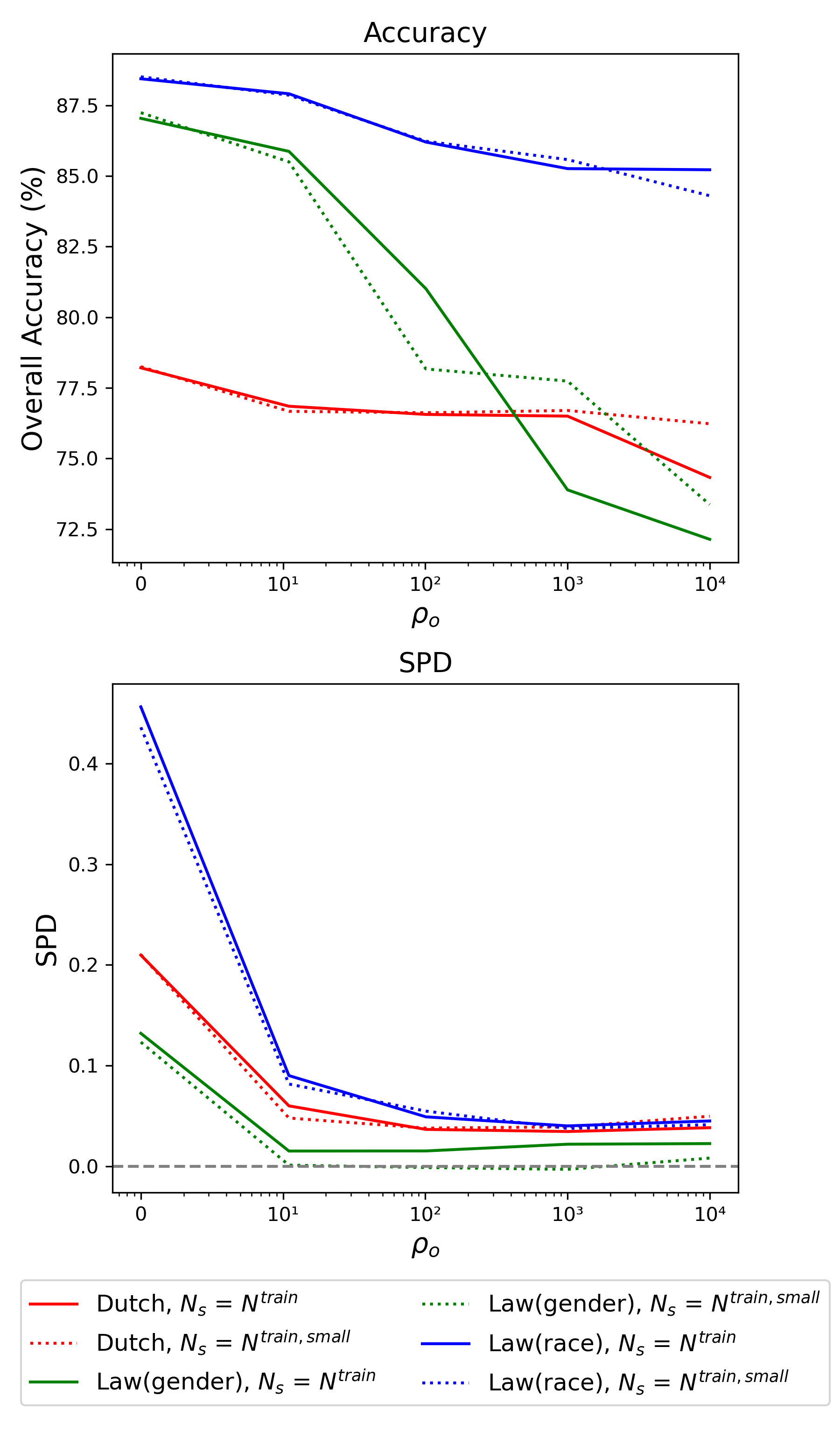
Ability of Preserving Privacy. To evaluate the possible effectiveness of our method in preserving client privacy while mitigating unfairness, we conducted experiments related to controlling the size of the synthetic dataset. For all of the tests in this section, we select , which is motivated by the numerical results in the previous section, and consider multiple values for to control the level of unfairness. We also set for the results obtained in this section.
First, we ran our framework with for each client so that the synthetic datasets learned are of the same size as their training data. Here we select , so that these synthetic data quantities are equal to their corresponding quantities in the training data (the synthetic quantities are learned using our framework).
Second, we ran our framework with and (see Table 1) so that the synthetic datasets are significantly smaller than the training sets (the synthetic datasets are about 10% of the size of the training sets). Here, are computed to have equal numbers ( of ) from each of the following sensitive feature and label pairs: , , , and . The quantities , which are learned in our framework, are initialized by sampling each feature from a normal distribution with mean and variance determined by the training data.
The results of our tests can be found in Table 2; see also the graphs in Figure 3. These empirical results show consistent performance trends for both accuracy and SPD, regardless of the synthetic dataset size or the initialization strategy; i.e., as we increase the penalty parameter , we sacrifice some accuracy while significantly improving fairness. Moreover, the difference in accuracy obtained when passing the significantly smaller dataset of size is similar to the accuracy obtained when passing a synthetic dataset that is the same size as the training dataset. We also remind the reader that the baseline setting of corresponds to ignoring fairness concerns, which is clearly illustrated in the poor values of SPD. Finally, the values of for all clients and datasets were in the range , thus showing that the synthetic datasets computed were significantly different from the training data. Overall, we believe these results provide evidence that our framework is able to offer good accuracy and acceptable unfairness measures for models obtained using relatively small synthetic datasets. Thus, our framework allows not only for the mitigation of unfairness but also the potential to protect client privacy through the use of small synthetic datasets.
5 Conclusion
In this study, we present a cost-effective communication strategy to mitigate unfairness and help preserve privacy across clients in an FL context. We propose to send a synthetic dataset from each client to the server instead of each client’s model. The manner in which we propose computing the synthetic dataset takes unfairness into account by solving a bilevel optimization problem. This allows the server to train a conventional ML model without further fairness concerns on the collection of client-provided synthetic datasets. This approach not only simplifies the training process for the server but also significantly reduces communication costs by limiting it to a one-time transfer between the clients and the server. Our implementation on well-known datasets illustrates that our approach effectively mitigates unfairness without sacrificing too much accuracy. Even with synthetic datasets of 10% the size of the client training data, our strategy remains effective in producing accurate models that are fair and aid in maintaining privacy.
References
- Buolamwini and Gebru (2018) Buolamwini, J.; and Gebru, T. 2018. Gender shades: Intersectional accuracy disparities in commercial gender classification. In Conference on fairness, accountability and transparency, 77–91. PMLR.
- Caton and Haas (2024) Caton, S.; and Haas, C. 2024. Fairness in machine learning: A survey. ACM Computing Surveys, 56(7): 1–38.
- d’Alessandro, O’Neil, and LaGatta (2017) d’Alessandro, B.; O’Neil, C.; and LaGatta, T. 2017. Conscientious classification: A data scientist’s guide to discrimination-aware classification. Big data, 5(2): 120–134.
- Dressel and Farid (2018) Dressel, J.; and Farid, H. 2018. The accuracy, fairness, and limits of predicting recidivism. Science advances, 4(1): eaao5580.
- Ezzeldin et al. (2023) Ezzeldin, Y. H.; Yan, S.; He, C.; Ferrara, E.; and Avestimehr, A. S. 2023. Fairfed: Enabling group fairness in federated learning. In Proceedings of the AAAI conference on artificial intelligence, volume 37, 7494–7502.
- Flaticon (2023) Flaticon. 2023. Illustration Icons. https://www.flaticon.com/. Accessed: 2023-06-02.
- Giovannelli, Kent, and Vicente (2024) Giovannelli, T.; Kent, G. D.; and Vicente, L. N. 2024. Bilevel optimization with a multi-objective lower-level problem: Risk-neutral and risk-averse formulations. Optimization Methods and Software, 1–23.
- Goetz and Tewari (2020) Goetz, J.; and Tewari, A. 2020. Federated learning via synthetic data. arXiv preprint arXiv:2008.04489.
- Hu et al. (2022) Hu, S.; Goetz, J.; Malik, K.; Zhan, H.; Liu, Z.; and Liu, Y. 2022. Fedsynth: Gradient compression via synthetic data in federated learning. arXiv preprint arXiv:2204.01273.
- Kim et al. (2021) Kim, E.; Bryant, D.; Srikanth, D.; and Howard, A. 2021. Age bias in emotion detection: An analysis of facial emotion recognition performance on young, middle-aged, and older adults. In Proceedings of the 2021 AAAI/ACM Conference on AI, Ethics, and Society, 638–644.
- Kingma (2014) Kingma, D. 2014. Adam: a method for stochastic optimization. arXiv preprint arXiv:1412.6980.
- Lohia et al. (2019) Lohia, P. K.; Ramamurthy, K. N.; Bhide, M.; Saha, D.; Varshney, K. R.; and Puri, R. 2019. Bias mitigation post-processing for individual and group fairness. In Icassp 2019-2019 ieee international conference on acoustics, speech and signal processing (icassp), 2847–2851. IEEE.
- McMahan et al. (2017) McMahan, B.; Moore, E.; Ramage, D.; Hampson, S.; and y Arcas, B. A. 2017. Communication-efficient learning of deep networks from decentralized data. In Artificial intelligence and statistics, 1273–1282. PMLR.
- Mehrabi et al. (2021) Mehrabi, N.; Morstatter, F.; Saxena, N.; Lerman, K.; and Galstyan, A. 2021. A survey on bias and fairness in machine learning. ACM computing surveys (CSUR), 54(6): 1–35.
- Mugunthan et al. (2021) Mugunthan, V.; Gokul, V.; Kagal, L.; and Dubnov, S. 2021. Bias-free fedgan: A federated approach to generate bias-free datasets. arXiv preprint arXiv:2103.09876.
- Obermeyer et al. (2019) Obermeyer, Z.; Powers, B.; Vogeli, C.; and Mullainathan, S. 2019. Dissecting racial bias in an algorithm used to manage the health of populations. Science, 366(6464): 447–453.
- Pan et al. (2023) Pan, Z.; Wang, S.; Li, C.; Wang, H.; Tang, X.; and Zhao, J. 2023. Fedmdfg: Federated learning with multi-gradient descent and fair guidance. In Proceedings of the AAAI Conference on Artificial Intelligence, volume 37, 9364–9371.
- Rasouli, Sun, and Rajagopal (2020) Rasouli, M.; Sun, T.; and Rajagopal, R. 2020. Fedgan: Federated generative adversarial networks for distributed data. arXiv preprint arXiv:2006.07228.
- Salazar et al. (2023) Salazar, T.; Fernandes, M.; Araújo, H.; and Abreu, P. H. 2023. Fair-fate: Fair federated learning with momentum. In International Conference on Computational Science, 524–538. Springer.
- Savard and Gauvin (1994) Savard, G.; and Gauvin, J. 1994. The steepest descent direction for the nonlinear bilevel programming problem. Operations Research Letters, 15(5): 265–272.
- Sinha, Malo, and Deb (2017) Sinha, A.; Malo, P.; and Deb, K. 2017. A review on bilevel optimization: From classical to evolutionary approaches and applications. IEEE transactions on evolutionary computation, 22(2): 276–295.
- Van der Laan (2001) Van der Laan, P. 2001. The 2001 census in the Netherlands: Integration of registers and surveys. In CONFERENCE AT THE CATHIE MARSH CENTRE., 1–24.
- Wang et al. (2018) Wang, T.; Zhu, J.-Y.; Torralba, A.; and Efros, A. A. 2018. Dataset distillation. arXiv preprint arXiv:1811.10959.
- Wang, Shu, and Culotta (2021) Wang, Z.; Shu, K.; and Culotta, A. 2021. Enhancing model robustness and fairness with causality: A regularization approach. arXiv preprint arXiv:2110.00911.
- Wightman (1998) Wightman, L. F. 1998. LSAC National Longitudinal Bar Passage Study. LSAC Research Report Series. Technical report, ERIC.
- Zafar et al. (2019) Zafar, M. B.; Valera, I.; Gomez-Rodriguez, M.; and Gummadi, K. P. 2019. Fairness constraints: A flexible approach for fair classification. The Journal of Machine Learning Research, 20(1): 2737–2778.
- Zafar et al. (2017) Zafar, M. B.; Valera, I.; Rogriguez, M. G.; and Gummadi, K. P. 2017. Fairness constraints: Mechanisms for fair classification. In Artificial intelligence and statistics, 962–970. PMLR.