The Asymptotics of Wide Remedians
Abstract
The remedian uses a matrix to approximate the median of streaming input values by recursively replacing buffers of values with their medians, thereby ignoring its most extreme inputs. Rousseeuw & Bassett (1990) and Chao & Lin (1993); Chen & Chen (2005) study the remedian’s distribution as and as . The remedian’s breakdown point vanishes as , but approaches as . We study the remedian’s robust-regime distribution as , deriving a normal distribution for standardized (mean, median, remedian, remedian rank) as , thereby illuminating the remedian’s accuracy in approximating the sample median. We derive the asymptotic efficiency of the remedian relative to the mean and the median. Finally, we discuss the estimation of more than one quantile at once, proposing an asymptotic distribution for the random vector that results when we apply remedian estimation in parallel to the components of i.i.d. random vectors.
1 Introduction
The word remedian refers to a collection of algorithms that take univariate input values and recursively whittle this down to values, where the last value estimates some inner quantile. As originally designated, the algorithm uses a matrix to approximate the median of data as they stream in (Rousseeuw & Bassett (1990)). Other formulations are possible:
- •
- •
The central idea—quantile estimation using recursion—predates the word itself (Tukey (1978); Weide (1978)).
- Note:
-
This code works so long as ; we recommend using odd
- Inputs:
-
-
1.
Remedian summarizing
-
2.
Data value
-
1.
- Output:
-
Remedian summarizing
- Let
-
and
- For
-
:
- If
-
:
- Let
-
- Let
-
- Let
-
for each
We focus on approximating the median of univariate data as they stream in. The streaming model of computation consists of a data source that emits one data point at a time and a core algorithm that receives each data point, carries out some computation, adjusts its internal storage state, and—forgetting the data point—stands ready to receive the next data point. The remedian—with internal storage state the matrix —is an elegant example of streaming computation. Numerous organizations use streaming computation to streamline the computation of realtime information and cut down on storage costs.
- Input:
-
Remedian
- Outputs:
-
-
1.
The remedian of the values summarized by
-
2.
The number of values summarized by
-
3.
The such that
-
1.
- Let
-
and
- Let
-
and
- For
-
:
- If
-
:
- Let
-
- Let
-
- Let
-
- Let
-
- Let
-
be an ordered list of the elements in
- Let
-
be the corresponding list of weights
- Let
-
- Return
-
, ,
The remedian uses the following approach:
-
1.
The remedian’s internal storage state, the matrix , starts out empty. Each cell initially contains the symbol NA (Table 2).
-
2.
Insertion is recursive: Row 1 receives raw data values from the data source, row 2 receives the medians of raw data values, row 3 receives the medians of the medians of raw data values, etc. When row () is full, it places the median of its values into the first empty cell in row and returns all of its cells to the empty state (Algorithm 1).
-
3.
The remedian estimate is the weighted median of the values in , where we note that a value in row represents input values (Algorithm 2). In theoretical settings (as here) the remedian estimate is the value the th row sends on to the nonexistent st row, i.e., the remedian returns this value right after the th insertion.
While the remedian ignores a positive fraction of its most extreme inputs, its finite-sample breakdown point falls between those of the mean and the median. Sending () sends the remedian’s breakdown point to zero (a limit between those for the mean and median). See §1.1.
1.1 How Robust is the Remedian?
Throughout we measure the robustness of an estimator using the breakdown concept of Hampel (1968).111Some authors feel estimators with large breakdown points hide important information in big data settings, favoring mixture modeling instead (see Huber & Ronchetti (2009) §11.1). That said, big data settings many times warrant the lightweight tracking we propose here. For finite , the breakdown point of an estimator is the smallest222The minimization occurs over the set of positions containing corrupted data values. fraction of the values that, when sent to infinity, corrupt the value of (Donoho & Huber (1983)). For example,
- Sample Mean
-
The breakdown point of is because for any .
- Sample Median
-
The breakdown point of
is . When (or, ), corrupting the median requires sending at least (or, ) values to infinity.
- Remedian
-
The breakdown point of the remedian when is
(1) Putting gives the sample median. When , corrupting the remedian requires sending at least second-row values to infinity, each of which requires sending at least first-row values to infinity. When , we must corrupt values, and induction gives (1).
For , , and , we have . Increasing remedian capacity by increasing the number of rows decimates robustness. In sections 3 and 4 we study the setting in which remains fixed while .
1.2 Previous Work
| Statistics | Computer Science | |
| Remedian | Tukey (1978) | Weide (1978) |
| Rousseeuw & Bassett (1990) | Battiato et al (2000) | |
| Chao & Lin (1993) | Cantone & Hofri (2013) | |
| Chen & Chen (2005) | ||
| Juritz et al (1983) | Shrivastava et al (2004) | |
| Quantile | Jain & Chlamtac (1985) | Agarwal et al (2013) |
| Estimation | Tierney (1993) | Karnin et al (2016) |
| on Data | Hurley & Modarres (1995) | Dunning & Ertl (2019) |
| Streams | Liechty et al (2003) | Masson et al (2019) |
| Chambers et al (2006) | Cormode et al (2021) | |
| + a few more | + many, many more |
While the remedian comes out of the statistics literature, the computer science literature has a great deal more to say about quantile estimation on data streams (Table 1). Rousseeuw & Bassett (1990) show that the remedian has breakdown point (1) and that the remedian’s estimate converges in probability to the population median under weak conditions as . Furthermore, they show that the standardized remedian converges to a non-Gaussian limiting distribution as . Chao & Lin (1993) and Chen & Chen (2005) continue this program, showing that the remedian’s estimate converges almost surely to the population median under weak conditions as or become large (see §2.4) and that the standardized remedian converges to normality as and both become large. Section 3.1 shows that this latter result holds when remains fixed and .
As noted, Battiato et al (2000); Cantone & Hofri (2013) describe a batch remedian that does its work in-place on an array of length . They develop an overly complex expression for the distribution of the remedian’s rank when . While their derivation assumes iid , its complexity makes it impossible to pursue for . In section 3.1 we derive the normal distribution of the remedian’s standardized rank when .
If we compare the computer science and statistics literatures on the topic of quantile estimation on data streams, the computer science literature has more to say, but the statistics literature does not lack for interesting results. Pearl (1981) describes a minimax tree: data percolate up from the leaves, undergoing alternating min and max operations. The value that reaches the root converges in probability to as the tree becomes tall. Krutchkoff (1986); Dunn (1991); Lau & Boos (1994) design size- algorithms that use the confidences intervals of Juritz et al (1983); Dudewicz & van der Meulen (1984). Tierney (1993) gives an online algorithm based on the stochastic approximation algorithm of Robbins & Monro (1951). Jain & Chlamtac (1985); Liechty et al (2003) use counting methods for approximating , which Raatikainen (1987, 1990); McDermott et al (2007) adapt to approximate (cf. §4.2). Hurley & Modarres (1995); Labo (2024) recommend using histograms.
We describe some recent results from the computer science literature.333See Cormode & Yi (2020) for a more detailed review of some of these algorithms. Shrivastava et al (2004) introduce Q-Digest, which assumes a universe of inputs and estimates rank to within units using space- trees. Agarwal et al (2013) describes compactors, sequences of buffers that, when full, send evenly- or oddly-indexed order statistics on to the next buffer. Karnin et al (2016) use these to design space- summaries that approximate rank to within units with probability , and Cormode et al (2021) use the same to design space-
summaries that approximate rank so that
Masson et al (2019) describe DDSketch, exponential histograms that guarantee
for space- summaries; see Labo (2024). Dunning & Ertl (2019) design -digest, a fixed-sized summary that uses a scaling function to focus attention on extreme quantiles.
1.3 Our Contributions
Symbol Meaning Notes unassigned or missing value as in R (R Core Team (2022)) is defined as or is assigned as see Algorithms 1 and 2 augmented reals positive integers possible remedian widths matrix Gamma function Beta function 1 if is true, 0 otherwise indicator function function composition converging sequence asymptotic equivalence cumulative distribution function convergence in distribution the distribution of RV stands for law , equality in distribution LHS, RHS abbreviations for the left- and right-hand sides of an equation iid or i.i.d. abbreviation for “independent and identically-distributed”
Organizations frequently ingest large, potentially-partially-corrupted data sets, wishing to cheaply, but robustly, monitor each data set’s central tendency. While the large- remedian uses space, it is not robust. The large- remedian, by contrast, is robust, but uses space. Organizations willing to spend more on storage for the sake of robustness should opt for the large- remedian. That said, while the literature describes the distributions of the large- and large- remedians, it does not yet describe the same for the large- remedian (§1.2; Rousseeuw & Bassett (1990); Chao & Lin (1993); Chen & Chen (2005)). We derive the large- distribution of the standardized remedian estimate, which we use to derive the large- distribution of the standardized (mean, median, remedian, remedian rank) vector. After that we turn to the large- distribution of the standardized vector that results when we use remedians in parallel to simultaneously approximate distinct, internal quantiles.
Section 2 presents several preliminaries: important assumptions, a recursive formula for the remedian’s distribution, Bahadur’s formula, and the remedian’s almost sure convergence to the population median. Sections 3 and 4 present our core results. Section 3 shows that the standardized (mean, median, remedian, remedian rank) vector approaches normality and derives the asymptotic relative efficiencies between the mean, the median, and the remedian. Section 4 takes up a related topic, proposing an expression for the large- distribution of the standardized vector that results when we use remedians in parallel to approximate distinct, internal quantiles; we prove the case . Section 5 concludes, and Table 2 defines some important notation.
2 Preliminaries
While sections 3 and 4 present our core results, this section describes several preliminaries, namely, key assumptions, a recursive formula for the remedian’s distribution, Bahadur’s formula, and the remedian’s almost sure convergence to the population median.
2.1 Assumptions
Throughout this paper we assume that
| (2) |
for CDF . While our results are nonparametric (Hollander et al (2014)), they require a well-behaved . For the remedian in section 3 our results require that
| (3) |
for the population median. More generally, for the remedian in section 4 our results require that
| (4) |
for the th population quantile. In general we require a continuous, positive, bounded density , and a bounded , on a neighborhood containing the estimand.444The requirement involving , atypical in this setting, comes from Bahadur (1966).
2.2 The Remedian’s Distribution
Let give the order statistics, a sorted rearrangement of the i.i.d. values in (2) (David & Nagaraja (2003)).555To obtain a unique sorted list, one can first sort by the indices, and then by the values. It is well-known that
| (5) |
for and the CDF. In particular, with , , and , , where
| (6) |
is the CDF. (Table 2 defines .) By the same reasoning, the remedian of values has distribution , so that, in general, the remedian of values has distribution , where
| (7) |
for (Rousseeuw & Bassett (1990)). Throughout we let represent the remedian’s rank among the i.i.d. , so that, in summary, we have
2.3 Bahadur’s Formula
In the sequel Lemma 2.1 from Bahadur (1966) aids in the proofs of results both well-known (Corollaries 2.2, 2.3, and 4.1) and new (Theorem 3.6). One further suspects that Lemma 2.1 will play a role in proving Conjectures 4.2 and 4.5.
Proof.
This is the central result of the excellent Bahadur (1966). ∎
Lemma 2.1 implies that almost surely (a.s.), as .
Proof.
Lemma 2.1 implies that almost surely, as , where the limit uses Slutsky’s theorem and the SLLN. ∎
Lemma 2.1 further implies that , as .
Proof.
Lemma 2.1 implies that , as , where the limit uses the CLT. ∎
2.4 The Remedian Converges with Probability One
Proof.
Theorem 2.4 in turn implies that almost surely, as .
3 Asymptotic Normality
While section 2.4 considers the almost sure convergence of and , section 3.1 shows that standardized and converge to normality. Section 3.2 further proves the asymptotic normality of the standardized (mean, median, remedian, remedian rank) vector, and section 3.3 studies the asymptotic efficiency of the remedian relative to the mean and the median.
3.1 Univariate Asymptotic Normality
We start with the asymptotic normality of the standardized remedian. While Corollary 2.3 implies that
replacing with on the LHS replaces 1 with on the RHS.
Proof.
Our asymptotic results reflect that the remedian is the median when . After that, each additional remedian buffer increases the asymptotic variance of the remedian over that of the median by an additional factor of to account for the increasing noisiness of as grows (cf. Theorem 3.3).
3.1.1 The Iterated Remedian
Say we have, not one remedian matrix (as above), but remedian matrices , where , for . What is the distribution of the estimate that results when we string these together, so that the output of becomes the input of , ? In particular, we imagine that:
-
1.
For , the i.i.d. inputs flow into the first row of ;
-
2.
For , the outputs of flow into the first row of ; and
-
3.
The output of , which we call , gives us our final estimate.
The following lemma shows that, if , for , then
3.1.2 The Remedian’s Rank
| 1 | 2 | 3 | 4 | 5 | 6 | 7 | 8 | 9 | |
| 0 | 0 | 0 | 3 | 8 | 3 | 0 | 0 | 0 |
Interest in dates to Tukey (1978); Rousseeuw & Bassett (1990). Tukey (1978) in particular uses combinatorics to derive (Table 3). Cantone & Hofri (2013) generalize this, deriving a complex expression for . We generalize this in the direction of wide remedians, deriving a simple expression for , which holds for any .
Noting that confirms the result for (cf. Theorem 3.1). For large, we have
so that, in this setting, the mean and variance of grow exponentially in , as expected. Note that, given the ranks of the , the remedian’s rank follows deterministically; i.e., depends on only through . The order statistics provide no additional information: does not depend on (cf. Theorem 3.1).
Finally, while Cantone & Hofri (2013) study (see Tables 3 through 5), we note that:
Definition 3.4.
For , is half-normal with and (Leone et al (1961)), i.e., .
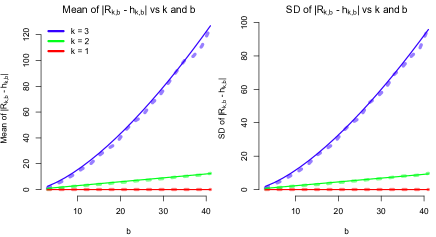
While our results assume large (Figure 1), they complement and expand on those in Cantone & Hofri (2013), who focus on .
3.2 Multivariate Asymptotic Normality
Above we consider the univariate convergence of the standardized median (§2.3), remedian (§3.1), and remedian rank (§3.1.2). The central limit theorem (CLT) gives the univariate convergence of the standardized mean . We now show that the standardized (mean, median, remedian, remedian rank) vector approaches quadrivariate normality. In so doing we derive the asymptotic correlations between all pairs of standardized variables.
Proof.

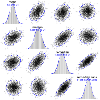
Figure 2 shows simulated mean, median, remedian, and remedian rank values when , , and ,666For positive and the distribution has and illustrating Theorems 3.1, 3.3, and 3.6. Simulated (pairs of) values (in gray) approximately follow their derived distributions (in blue). Replacing with, e.g., (which has infinite mean and variance) produces plots with outlying , but normally-distributed medians, remedians, and remedian ranks. The remedian with uses 74.3% of its central inputs (§1.1). Theorem 3.6 holds for its last three variables when while the streaming computation of stores only two numbers: and .
The standardized variables above have the following limiting correlations:
Corollary 3.7.
If and has the large- distribution on the RHS of (13), then has correlation matrix
The normality of the , , then implies the following large- dependencies:
Example 3.8.
Remark 3.9.
While Theorem 3.6 includes three measures of location—the mean, median, and remedian, Corollary 3.10 studies the differences of pairs of these as . We ask, e.g., how well does the remedian approximate the sample median?
When (i.e., the remedian is the median), the variance in (14) equals zero and the variances in (15) and (16) equal each other, as desired (cf. Theorems 3.1 and 3.3). By (14), the remedian’s error in approximating the sample median approaches zero in probability, as , at rate , where . Panels (15) and (16) describe systematic () and stochastic (of order ) errors in using the median or the remedian to approximate the sample mean, the former vanishing when . Finally, and Remark 3.9 imply that:
That is to say, the variances in (15) and (16) make sense (i.e., are non-negative); also, the variance in (16) exceeds that in (15) when , as expected.
3.3 Asymptotic Relative Efficiency
Theorem 3.6 in hand, we now ask, which of its three, asymptotically-unbiased measures of location most efficiently uses its data points to approximate the estimand of interest, the population median ? Statements comparing the efficiencies of estimators depend on the distribution . The fact below assumes normality, which implies that .
Fact 3.11.
For known and ,
-
1.
The Fisher information in about is ;
-
2.
The sample mean efficiently estimates ; and
-
3.
When , the sample median, , is as efficient as in estimating .
Proof.
While the tails of the normal distribution quickly approach zero, the sample mean efficiently estimates its center, . By the Cramér-Rao lower bound, provides a lower bound for the variance of any unbiased estimator of (part 2). The sample median squanders of its data, as ; the asymptotic relative efficiency (ARE) of relative to is
(see Corollary 2.3). Equivalently, , as (part 3). The ARE measures the efficiency of one estimator relative to another, under a certain , as . Efficient estimators quickly zero in on their estimands.
While Fact 3.11 gives under normality, Propositions 3.12 and 3.13 give and under any satisfying (3).
Proposition 3.12.
Proof.
As expected, the remedian’s efficiency falls below that of the sample median when (Theorems 3.1 and 3.3). The following proposition assumes .
Proposition 3.13.
Proof.
While Proposition 3.13 generalizes part 3 of Fact 3.11,777It includes both the median and the remedian, and it holds for any satisfying (3). it has more moving parts: loses efficiency relative to when increases, decreases, or decreases. The following corollary studies three symmetric distributions.
Corollary 3.14.
Let have a -distribution with degrees of freedom and fix . Proposition 3.13 implies that:
-
1.
If , the remedian is
as efficient as the sample mean in estimating as .
-
2.
If , the remedian is
as efficient as the sample mean in estimating as .
-
3.
If , the remedian is as efficient as the sample mean in estimating as .
Note that Proposition 3.13 implies Corollary 3.14.3 implies Fact 3.11.3 and that Corollary 3.14 parts 1 and 2 include two interesting extremes:
-
1.
If and , the efficiency of infinitely exceeds that of because ;
-
2.
If and , the efficiency of infinitely exceeds that of because , producing many outliers (imagine Figure 2 with data).
4 Asymptotic Normality of General Estimators
While our paper so far focuses on estimating the population median , we now turn to general estimands: , for ; see (4). In particular, we propose an asymptotic distribution for the low-memory estimator that results when we use the remedian to estimate the quantiles (see Conjecture 4.5). We prove the case . Section 4.1 gives preliminaries to our approach, which expands on an idea from Chao & Lin (1993); see section 4.2.
4.1 Medians and Remedians of Vector Components
The following corollary of Lemma 2.1 gives the limiting distribution of the vector that holds the sample quantiles of the components of i.i.d. random vectors.
Corollary 4.1.
Proof.
While Corollary 4.1 applies, e.g., the median to the components of the , we now consider what happens when we replace the median with the remedian. The median to remedian analogy of Corollary 2.3 to Theorem 3.1 suggests that:
Conjecture 4.2.
4.2 Remedian Estimates for Multiple Quantiles
Chao & Lin (1993) describe the following remedian-based estimator of , for any . Start by finding for which
| (20) |
for as in (5). Fixing and , we add a buffer of size above the usual remedian. With , we imagine a streaming setting in which the data points i.i.d. first enter the -buffer. Whenever the -buffer becomes full, it passes its th order statistic on to the first row of the remedian and reverts to the empty state. Let and
Then, putting and citing §1.1 and §2.2, we have
| (21) |
for the finite- breakdown point and distribution of . With data from we obtain the following corollaries of Theorems 2.4 and 3.1.
Results like these, with in the latter case, appear in Chen & Chen (2005). The following multivariate proposal moves beyond Chen & Chen (2005):
Conjecture 4.5.
Proof.
Apply Conjecture 4.2 noting that the gaps between the are . ∎
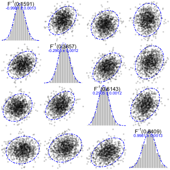
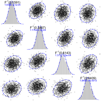
While organizations often wish to track quantiles (Raatikainen (1987, 1990); McDermott et al (2007); Chambers et al (2006)), Conjecture 4.5 proposes a distribution for the large-, remedian-based estimate of quantiles. While Conjecture 4.2 implies Conjecture 4.5 and Figure 3 simulates quantities from Conjecture 4.5, the results in Figure 3 support both conjectures. It is worth noting that an implementation of Conjecture 4.5 in the streaming setting requires space, as . Finally, the -remedian of Conjecture 4.5 has breakdown point (cf. (21)).
5 Conclusions and Discussion
Our paper adds to our understanding of the remedian, a low-memory estimator of . As (as ) the remedian uses space ( space) and 100% (100%) of its central inputs (§1.1). With , we derive the distribution of the standardized (mean, median, remedian, remedian rank) vector (§3.2); compare the efficiencies of the mean, median, and remedian (§3.3); and propose a distribution for the remedian estimate of population quantiles, proving the case for (§4.2). We contextualize the sample median, i.e., the remedian with . As increases, estimators become more variable, less efficient, and less robust.
The remedian presents an interesting setting in which to study how memory requirements trade off against robustness, efficiency, and precision. Where—one might ask—does the remedian fit into the panoply of techniques for streaming quantile estimation (Table 1)? The remedian is distinguished by its robustness and our understanding of how it interacts with population and sample quantities (e.g., Theorem 3.6 and Corollary 3.10). The large- remedian, with its non-zero breakdown point and relatively large size, is the Cadillac of quantile estimators: big and roomy, but expensive. An organization might use the -remedian (§4.2) to track important, but potentially-corrupted, data streams.
References
- Agarwal et al (2013) Agarwal PK, G Cormode, Z Huang, JM Phillips, Z Wei, K Yi (2013) “Mergeable Summaries.” ACM Transactions on Database Systems, 38:4:26, pages 1–28.
- Babu & Rao (1988) Babu GJ & CR Rao (1988) “Joint asymptotic distribution of marginal quantiles and quantile functions in samples from a multivariate population.” J of Multivariate Analysis, 27(1): pages 15–23.
- Bahadur (1966) Bahadur RR (1966) “A note on quantiles in large samples.” Ann. Math. Statist., 37(3): pages 577–580.
- Battiato et al (2000) Battiato S, D Cantone, D Catalano, G Cincotti, M Hofri (2000) “An efficient algorithm for the approximate median selection problem.” Eds. G Bongiovanni, R Petreschi, G Gambosi. Algorithms and Complexity: Proceedings of the 4th Italian Conference, CIAC 2000, Rome, Italy, pages 226–238.
- Billingsley (1995) Billingsley P (1995) Probability and Measure, 3rd Edition. Wiley, New York, NY.
- Cantone & Hofri (2013) Cantone D & M Hofri (2013) “Further analysis of the remedian algorithm.” Theoretical Computer Science, 495: pages 1–16.
- Chambers et al (2006) Chambers JM, DA James, D Lambert, S Vander Wiel (2006) “Monitoring networked applications with incremental quantile estimation.” Statistical Science, 21(4): pages 463–475.
- Chao & Lin (1993) Chao MT & GD Lin (1993) “The asymptotic distributions of the remedians.” Journal of Statistical Planning and Inference, 37: pages 1–11.
- Chen & Chen (2005) Chen H & Z Chen (2005) “Asymptotic properties of the remedian.” Nonparametric Statistics, 17(2): pages 155–165.
- Cormode et al (2021) Cormode G, Z Karnin, E Liberty, J Thaler, & P Veselý (2021a) “Relative error streaming quantiles.” Proc PODS ’21, Virtual Event, China.
- Cormode & Yi (2020) Cormode G & K Yi (2020) Small Summaries for Big Data. Cambridge UP, Cambridge, UK.
- David & Nagaraja (2003) David HA & HN Nagaraja (2003) Order Statistics, 3rd Edition. Wiley, Hoboken, NJ.
- Donoho & Huber (1983) Donoho DL & PJ Huber (1983) “The notion of breakdown point.” In A Festschrift for Erich L. Lehmann, PJ Bickel, KA Doksum, JL Hodges, Eds, Wadsworth, Belmont, CA.
- Dudewicz & van der Meulen (1984) Dudewicz & van der Meulen (1984) “On assessing the precision of simulation estimates of percentile points.” American Journal of Mathematical and Management Sciences, 4(3-4): pages 335–343.
- Dunn (1991) Dunn CL (1991) “Precise simulated percentiles in a pinch.” The American Statistician, 45(3): pages 207–211.
- Dunning & Ertl (2019) Dunning T & O Ertl (2019) “Computing Extremely Accurate Quantiles Using t-Digests.” See https://arxiv.org/abs/1902.04023.
- Englund (1980) Englund G (1980) “Remainder term estimates for the asymptotic normality of order statistics.” Scandinavian Journal of Statistics, 7: pages 197–202.
- Hampel (1968) Hampel FR (1968) Contributions to the theory of robust estimation, PhD Thesis, Department of Statistics, University of California, Berkeley.
- Hollander et al (2014) Hollander M, DA Wolfe, E Chicken (2014) Nonparametric Statistical Methods. Wiley, Hoboken, NJ.
- Huber & Ronchetti (2009) Huber PJ & EM Ronchetti (2009) Robust Statistics, 2nd Edition. Wiley, Hoboken, NJ.
- Hurley & Modarres (1995) Hurley C & R Modarres (1995) “Low-storage quantile estimation.” Computational Statistics, 10: pages 311–325.
- Jain & Chlamtac (1985) Jain R & I Chlamtac (1985) “The algorithm for dynamic calculation of quantiles and histograms without storing observations.” Communications of the ACM, 28(10): pages 1076–1085.
- Juritz et al (1983) Juritz JM, JWF Juritz, MA Stephens (1983) “On the accuracy of simulated percentile points.” JASA, 78(382): pages 441–444.
- Karnin et al (2016) Karnin Z, K Lang, E Liberty (2016) “Optimal quantile approximation in streams.” Proc IEEE FOCS ’16, pages 71-78.
- Krutchkoff (1986) Krutchkoff (1986) “C262. Percentiles by simulation: reducing time and storage.” Journal of Statistical Computation and Simulation, 25(3-4): pages 304–305.
- Labo (2024) Labo P (2024) “Using exponential histograms to approximate the quantiles of heavy- and light-tailed data.” https://arxiv.org/abs/2404.18024
- Lau & Boos (1994) Lau L-C & DD Boos (1994) “A fast and low-storage algorithm for finding quantiles.” NC State Institute of Statistics Mimeo Series #2268.
- Lehmann & Casella (1998) Lehmann EL & G Casella (1998) Theory of Point Estimation, 2nd Edition. Springer, New York, NY.
- Leone et al (1961) Leone F C, LS Nelson, RB Nottingham (1961) “The folded normal distribution.” Technometrics, 3(4): pages 543–550.
- Liechty et al (2003) Liechty JC, DKJ Lin, JP McDermott (2003) “Single-pass low-storage arbitrary quantile estimation for massive datasets.” Statistics and Computing, 13: pages 91–100.
- Mallows (1991) Mallows C (1991) “Another comment on O’Cinneide.” The American Statistician, 45(3): page 257.
- Masson et al (2019) Masson C, JE Rim, HK Lee (2019) “DDSketch: a fast and fully-mergeable quantile sketch with relative-error guarantees.” Proc VLDB Endowment, 12: 12.
- McDermott et al (2007) McDermott JP, GJ Babu, JC Liechty, DKJ Lin (2007) “Data skeletons: simultaneous estimation of multiple quantiles for massive streaming datasets with applications to density estimation.” Stat Comput, 17: pages 311–321.
- Pearl (1981) Pearl J (1981) “A space-efficient on-line method of computing quantile estimates.” Journal of Algorithms, 2(2): pages 164–177.
- R Core Team (2022) R Core Team (2022) R: A language and environment for statistical computing. R Foundation for Statistical Computing, Vienna, Austria. https://www.R-project.org/.
- Raatikainen (1987) Raatikainen KEE (1987) “Simultaneous estimation of several percentiles.” Simulation, 49(4): pages 159–163.
- Raatikainen (1990) Raatikainen KEE (1990) “Sequential procedure for simultaneous estimation of several percentiles.” Transactions of the Society for Computer Simulation, 7(1): 21–44.
- Reiss (1989) Reiss R-D (1989) Approximation Distributions of Order Statistics. Springer Verlag, New York, NY.
- Robbins & Monro (1951) Robbins H & S Monro (1951) “A stochastic approximation method.” The Annals of Mathematical Statistics, 22(3): pages 400–407.
- Rousseeuw & Bassett (1990) Rousseeuw PJ & GW Bassett Jr (1990) “The remedian: a robust averaging method for large data sets.” Journal of the American Statistical Association, 89(409): pages 97–104.
- Schervish (1995) Schervish MJ (1995) Theory of Statistics. Springer Verlag, New York, NY.
- Shrivastava et al (2004) Shrivastava N, C Buragohain, D Agrawal, S Suri (2004) “Medians and beyond: new aggregation techniques for sensor networks.” SenSys ’04: Proceedings of the 2nd International Conference on Embedded Networked Sensor Systems, pages 239–249.
- Tierney (1993) Tierney L (1993) “A space-efficient recursive procedure for estimating a quantile of an unknown distribution.” SIAM Journal on Scientific and Statistical Computing, 4(4): pages 706–711.
- Tukey (1978) Tukey JW (1978) “The ninther: a technique for low-effort robust (resistant) location in large samples.” Contributions to Survey Sampling and Applied Statistics: Papers in Honor of H.O. Hartley, ed. HA David. Academic Press, pages 251–257.
- Weide (1978) Weide B (1978) “Space-efficient on-line selection algorithms.” Computer Science and Statistics: Proceedings of the Eleventh Annual Symposium on the Interface, pages 308–311.
Appendix A Proof of Theorem 3.1
Chen & Chen (2005) unwittingly show that the standardized remedian converges to normality as and remains fixed. The statement they prove sends both and to infinity, but their proof works when just . We present a slightly modified version of their proof, starting with the following four facts and three lemmas, which appear in Chen & Chen (2005). In what follows let
| (22) |
be the height of the density at for and .
Fact A.1.
has fixed points at , i.e., , for .
Proof.
Let . Note that . Then, by induction on , we have . ∎
Fact A.2.
If , then .
Proof.
This is true for . Induction and Fact A.1 yield the result. ∎
Fact A.3.
For any ,
| (23) | ||||
| (24) |
Proof.
First, it is clear that , for all . Then, by induction on , we note that
| (25) | ||||
| (26) | ||||
| (27) | ||||
| (28) | ||||
| (29) |
where (27) uses the base case and the induction hypothesis and (28) uses Fact A.1.
Induction also shows that . Definition (22) gives the base case. For note that
Fact A.4.
as .
Proof.
Using Stirling’s approximation and , we have
∎
Lemma A.5.
For some generic and such that ,
Proof.
We proceed by induction, proving two base cases.
- Case k = 1
-
Expression (7) gives , so that .
- Case k = 2
- Induction on k 2
∎
Lemma A.6.
Let be the th order statistic of . For and , we have .888The argument in Chen & Chen (2005) uses, but does not prove, this statement.
Proof.
Lemma A.7.
For and , we have
for the th order statistic, the standard normal CDF, and .
See 3.1
Proof.
By Fact A.4, showing that suffices, where
| (42) |
We pursue the following in order to show that :
-
1.
We derive three Taylor series expansions and a limit using the last two;
-
2.
From Lemma A.7, the limit, and the first Taylor series we derive the result.
We first derive three Taylor series expansions:
- 1.
-
2.
We expand about :
(47) where is between and .
- 3.
We now derive the aforementioned limit. Using (49) and (42) we have
| (50) | ||||
| (51) |
where (51) uses Lemma A.5 (which uses (47) and (42) to show that ) and (4).
Appendix B Proof of Lemma 3.2
We now prove our iterated remedian result, starting with the following fact.
Fact B.1.
is continuous.
Proof.
, the integral of a continuous function, is continuous. is continuous by induction: the composition of two continuous functions is continuous. ∎
See 3.2
Proof.
Fact B.1 and assumption (3) imply that is continuous on an open interval containing . Noting that
for large enough, we see that the multivariate limit in (10) exists. We proceed by induction on . Theorem 3.1 gives the base case . Assuming that
| (56) |
for , we have
| (57) | |||
| (58) | |||
| (59) |
where the first expression in (58) uses Fact B.1 and (56), and (59) uses Theorem 3.1. This completes the proof. ∎
Appendix C Proof of Theorem 3.3
We turn the the asymptotic normality of the remedian rank , starting with three lemmas. The latter two are well-known and proved here for completeness.
Lemma C.1.
For and let
For every there is a sequence of values such that , for , and .
Proof.
Consecutive elements in are one unit apart, which implies that consecutive elements in are units apart. Further, we note that
so that, for large enough and , contains elements both larger than and smaller than . This completes the proof. ∎
Lemma C.2.
If , , and ,
Proof.
Let . Next, for , let
so that and are independent, and
Then,
| (60) | ||||
| (61) |
The first term in the numerator of (61) equals
| (62) | ||||
| (63) |
The second term in the numerator of (61) equals
| (64) | ||||
| (65) |
Summing (63) and (65) we see that equals
| (66) |
To see that (66) converges to , note that
-
1.
The denominator converges almost surely to one (SLLN);
-
2.
, for (CLT);
-
3.
, for (CLT);
-
4.
implies , where indicates independence;
-
5.
Numerator of (66) (independence);
-
6.
.
While the numerator of (66) converges to and the denominator converges almost surely to one, Slutsky’s theorem gives the desired result. ∎
Lemma C.3.
.
Proof.
See 3.3
Proof.
With the result holds when , so assume that . For , Theorem 3.1 gives
| (73) |
For and
let be a sequence of values such that , for , and (see Lemma C.1), and let
| (74) |
Then, implies that and
because . Then, Lemma C.2 999Use and Slutsky’s theorem. gives
| (75) |
Finally, panels (73) through (75) and Lemma C.3 give the desired result. ∎
Appendix D Proof of Theorem 3.6
We close by deriving the quadrivariate limit in Theorem 3.6. Note that the limit for the last three variables holds when .
See 3.6
Proof.
This is true for . We assume . By the Cramér-Wold theorem (Billingsley (1995), page 383), the result follows if we can show that as , where ,
| (76) |
and
For and
let be a sequence of values such that , for , and (see Lemma C.1). Further, let
As , Lemma 2.1 then gives
| (77) | |||
| (78) |
where (77) uses the CLT, Slutsky’s theorem, , and (3), and (78) uses
| (79) | ||||
To summarize, we have
| (80) | ||||
| (81) |
where (80) uses and defined by (78), and (81) uses as in Theorem 3.3. Letting and , we finally have
so that , for as in (76), completing the proof. ∎