Graph-based Signal Sampling with Adaptive Subspace Reconstruction for Spatially-irregular Sensor Data
Abstract
Choosing an appropriate frequency definition and norm is critical in graph signal sampling and reconstruction. Most previous works define frequencies based on the spectral properties of the graph and use the same frequency definition and -norm for optimization for all sampling sets. Our previous work demonstrated that using a sampling set-adaptive norm and frequency definition can address challenges in classical bandlimited approximation, particularly with model mismatches and irregularly distributed data. In this work, we propose a method for selecting sampling sets tailored to the sampling set adaptive GFT-based interpolation. When the graph models the inverse covariance of the data, we show that this adaptive GFT enables localizing the bandlimited model mismatch error to high frequencies, and the spectral folding property allows us to track this error in reconstruction. Based on this, we propose a sampling set selection algorithm to minimize the worst-case bandlimited model mismatch error. We consider partitioning the sensors in a sensor network sampling a continuous spatial process as an application. Our experiments show that sampling and reconstruction using sampling set adaptive GFT significantly outperform methods that used fixed GFTs and bandwidth-based criterion.
Index Terms— graph sampling, sampling set adaptive GFT, spectral folding, sensor network, spatial continuous process
1 INTRODUCTION
Graph signal sampling and interpolation involve observing a signal at of the graph nodes and using graph models to produce an interpolated signal at the remaining nodes [1]. Since the sampled signal lies in an -dimensional space, when using linear interpolators, the reconstructed signal belongs to an -dimensional subspace of the original -dimensional space. Existing works typically fix this subspace a priori (e.g., the span of the first basis vectors of the GFT) for all sampling sets [2, 3, 4, 5, 6, 7, 8, 9, 10]. This raises the question of how to optimize sampling strategies when a suitable subspace prior is not available for the data. While in standard graph models signals that are smooth with respect to the graph (low-frequency signals) are assumed to be more likely, this does not mean that a subspace approximation (assuming only the first frequencies are non-zero) is desirable. In particular, in our previous work [11], we showed that even if the original signal is smooth, the signal obtained by introducing zeros in unobserved nodes has potentially large energy in arbitrary frequencies, so a simple low-pass filter reconstruction produces poor results. As an alternative, we proposed designing a sampling set-dependent GFTs and corresponding reconstruction subspaces for which low pass filtering yields robust reconstruction, outperforming standard approaches [2, 3, 4, 5, 6, 7, 8, 9, 10, 12]. While in [11], we assumed the sampling set was given, here we address sampling set selection.
Our work is based on the irregularity-aware graph Fourier transform [13], which allows for selecting an inner product as an additional degree of freedom to define different frequency representations of signals. In [14], the authors proposed using an alternate norm (independent of the sampling set) for sampling and reconstruction that can take into account the irregularities in a sensor network capturing a spatially regular signal. In their experiments, they observed that different norms and corresponding frequency definitions could yield different reconstruction performances for different sampling sets [14]. In our previous work [11], we introduced a sampling set-adaptive norm that can account for irregularities: 1) the relative contribution of sampled nodes for interpolation, and 2) the relative reliability of interpolated nodes. We showed that this interpolation can yield a robust reconstruction compared to the other methods that use standard sampling set-independent norm for optimization, particularly in the presence of model mismatches.
In this work, we assume that the graph Laplacian approximates the inverse covariance of the data and that the signals have a decaying power spectrum. We use the interpolator from [11], which is based on a reconstruction subspace that is a function of the sampling set and is not fixed a priori. We show that this interpolation error depends only on the higher frequency content of the original signal as a function of the sampling set. Based on this, we compute the covariance of energy in the high frequencies and formulate the sampling set selection problem as an E-optimal design [2]. Furthermore, we show that the optimal linear Gauss Markov random field (GMRF) estimator can be interpreted as a subspace reconstruction with the sampling-set-adaptive frequency definition. From this, we justify how our reconstruction method can mitigate the effects of model mismatches for non-GMRF data.


As a use case, we address the problem of finding multiple sampling subsets for sensor networks sampling a spatial process [15, 16, 17]. First, we collect data from all sensors over a duration of and learn a graph model. In this scenario, the learned graph may not capture the statistics of the underlying data (which was produced by a continuous process independent of the sensor locations) and provide only an approximation of the model. We then identify multiple disjoint sampling subsets as illustrated in Fig. 1a. In practice, these subsets alternatively sample during different time frames and the readings of non-sampled sensors are interpolated, as shown in Fig. 1b. This minimizes sensor active time and extends the sensor lifetime. We compare the interpolation performance to the state-of-the-art bandlimited reconstruction method [15], showing that our approach outperforms the state-of-the-art by approximately dB when interpolating signals varying rapidly in space with fewer samples.
2 Preliminaries
2.1 Graph signals and -GFTs
Let denote a undirected graph, where is the vertex set, and is the edge set. A graph signal is a function , with vector representation given by , where is the signal value at vertex . The graphs are represented by a positive semi-definite variation operator , where is the weight of the edge between vertex and , and , whenever . The variation operator measures signal smoothness in a Hilbert space where the inner product is defined as with induced -norm where . The -GFT [13] is defined as the generalized eigenvectors of which solves , where are the graph frequencies and the columns of forms a -orthonormal (i.e., ) basis for . This corresponds to the decomposition , where . The -GFT representation of a signal is defined as and the corresponding inverse transform is given by .
2.2 Bandlimited graph signal interpolation
Given a signal and a sampling set , the bandlimited reconstruction aims to interpolate from in the form , where and . The sample consistent bandlimited interpolation is obtained as [14]
| (1) |
The sampling set selection methods aim to find the optimal sampling set that minimizes the effect of model mismatch and/or noise [1, 14].
In our previous work [11], we introduced a sampling set-adaptive interpolation with a specific choice of , which results in graph frequencies exhibiting a property known as spectral folding (SF)[18]. We say that -GFT has the spectral folding property if for any generalized eigenpair of the -GFT, is also a generalized eigenpair of the -GFT (i.e., ). Here, , is a partition, and is a diagonal matrix with diagonal entries given by and . Furthermore, the -GFT has the spectral folding property iff the inner product is chosen as111We use the notation to emphasize that is a function of .
| (2) |
Note that this -GFT is a function of , meaning the subspace for signal interpolation depends on the sampling set. Furthermore, leveraging the spectral folding property and letting , the reconstruction formulae in (1) simplify to [11]
| (3) |
Note that the -norm of the signal takes the relative contribution of the sampled nodes for the reconstruction and relative reliabilities of interpolation in non-sampled nodes into account [11].
3 Sampling set selection
3.1 Sampling set selection
Let be a random signal drawn from a distribution with covariance , with , and let be selected according to (2). We formulate the sampling set selection problem as choosing the subset that minimizes the worst-case bandlimited model mismatch error (E-optimal) of the signal with respect to the -GFT interpolator with SF introduced in [11].
We first define three frequency domain subspaces associated with the SF -GFT. We define , , and , for low, middle and high frequency signals, respectively. The index sets associated to each sub-space are , , and . Without loss of generality, we assume that and that has full row rank, i.e., . It can be proved that and [18]. Note that these subspaces and frequencies are functions of .
Any signal can be decomposed as , where is the bandlimited component, , and . Here, represents the bandlimited model mismatch error of the signal. Furthermore, let , where , , and .
Theorem 1.
If we use (3) to interpolate from , then the reconstruction error in -norm is given by
Proof.
Note that this property of folding higher-frequency energy into low-frequency (aliasing) while sampling is due to the SF property. Other GFTs spread the error across all frequencies while sampling, which makes it more challenging to isolate and minimize those errors [11]. The above result states that the reconstruction error with the interpolator in (3) depends only on the higher frequency component of the signal. Therefore, minimizing the energy in high-frequency as a function of effectively optimizes the frequencies for better energy compaction, which is favourable for the reconstruction in (3).
Theorem 2.
The covariance of the high-frequency transform coefficient is a diagonal matrix given by .
Proof.
| (5) |
The last equality follows from . ∎
It is worth noting that the covariance matrix simplifies to a diagonal matrix by choosing as in (2). Furthermore, this allows us to compare the worst-case high frequency error corresponding to different subspaces generated by different sampling sets of the same size in terms of .
Remark 1.
e can also show that and are uncorrelated, and is an -dimensional identity matrix. When the sampling set size is fixed, as is common in sampling set selection methods, becomes a constant, thus we can omit from the sampling set selection criteria.
Proposition 1.
The E-optimal sampling design minimizing the maximum singular value of is given by
Proof.
| (6) |
The last equality follows from the spectral folding property, where , with being the largest frequency of the SF -GFT that is smaller than . ∎
3.2 Relation to GMRF model
Assume . It is known that the minimum-mean square error (MMSE) estimation of the GMRF is given by . The following theorem establishes that the optimal MMSE estimation in a GMRF can be interpreted as a subspace reconstruction with subspace adaptive frequency definition222In this subsection, we use for ease of notation.:
Theorem 3.
In a GMRF, if we assume and is selected according to (2), then .
From the above theorem, we can infer that the MMSE estimator is a sampling set-adaptive subspace reconstruction. The only difference between MMSE estimator and the interpolator in (3) is the term . The diagonal entries of could be viewed as penalties on each of these frequencies. These bases and penalties come from the GMRF model as a function of . In the presence of model mismatches, the reliability of these subspaces and frequencies from the graph model becomes questionable. Because of this uncertainty, the interpolator in (3) does not penalize these frequencies and uses the same sampling set-adaptive subspace as the MMSE estimator. This intuition explains why the interpolator in [11] could work better for non-GMRF data in the presence of model mismatch.
Proof of Theorem 3.
Consider the following block-inverse formula:
| (7) |
where , and similarly for . We can observe that . Then, starting from the identity , consider the block-wise expansion of . We can show that , where . Then, using the spectral folding properties , , and , we can further simplify the above expression as follows:
| (8) |
∎
3.3 Representative sampling partitions
Given a sensor network with vertices , representative sampling subset partitioning involves finding a partition , where , such that each subset serves as a sampling set to reconstruct the signal in its complement . Based on (6) and following the algorithm proposed in [15], the algorithm we use for partitioning is outlined in Algorithm 1.
3.4 Efficient implementation
To reduce the computations associated with the inversion of , we use the following Neumann series expansion [19]:
| (9) |
where is a diagonal matrix with , and is non negative with zero diagonal. The zero-order approximation of is given by , and similarly, . Using (8), we can show that . Then, the approximated version (6) is given as follows:
| (10) |
In step of Algorithm 1, we solve (10) instead of (6) for efficient computations.We solve this problem using a greedy approach, similar to other greedy sampling methods in the GSP literature [1, 4].
4 EMPIRICAL RESULTS
We use a synthetic example of a sensor network capturing spatial Gaussian processes to demonstrate the efficiency of the proposed partitioning method. We compare against [15, Algorithm 4], which optimizes the partition under the assumption of a bandlimited model for signals on graphs, as it is more comparable to our approach. We use the following error metric from [15] to compare the partitions obtained from different methods:
| (11) |
where is the number of signals used to evaluate the performance.
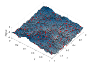
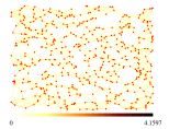
We consider a dense grid within a square in and consider Gaussian process with covariance to model a continuous process in space, where . Here, represents the Euclidean distance between points and , and is a parameter controlling the smoothness of the signal. Then, we select random locations within the square to simulate the sampling of the Gaussian process using sensors. These sensor locations are fixed throughout all the experiments in this section. A realization of the Gaussian process and sensor locations are shown in Fig. 2a. We denote the signal to be measured by . We generate independent identically distributed (i.i.d.) realizations of and obtain its sample covariance matrix . The graph for the sensor network is a combinatorial graph Laplacian learned from this covariance matrix using [20, Algorithm 2]. This graph is constrained so that the sensors are connected only to their neighbours within a radius of . The sensor network graph learned for the smoothness parameter (smooth variation in space) is shown in Fig. 2b.
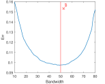
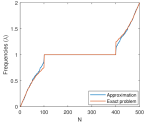
The method in [15] requires the bandwidth of the signals as an input for the algorithm. To estimate the bandwidth for the bandlimited model with respect to -GFT, we use the same signals employed for learning the graph. First, we generate a partition with using [15, Algorithm 4], assuming the bandwidth is . Then, we reconstruct all the signals in the training set using each subset in the partition for various bandwidths and compute the error metric given in (11). The plot of versus bandwidth for the data corresponding to is shown in Fig. 3a. The optimal bandwidth, , for reconstruction is identified as the bandwidth that minimizes the reconstruction error [21]. Furthermore, we observed the frequencies obtained by solving the exact problem in (6) and its approximation in (10) for , as shown in Fig. 3b. This shows that our approximation is reasonably accurate for solving (6).
We chose such that , to ensure that all subsets can achieve near-optimal reconstruction with -GFT bandlimited reconstruction. We obtain the representative sampling partitions using Algorithm 1 and [15, Algorithm 4], for different values of , and . The value obtained for -GFT bandlimited reconstruction for and are and respectively. The average SNR obtained over test signals for each case with these partitioning and reconstruction methods are shown in Table 1. From the table, we observe that for smooth signals with , the proposed method outperforms the competing method by 2 dB. In a more challenging scenario, where the signal varies rapidly in space () and , our method exceeds the competitor by approximately 4 dB. Furthermore, the small gain observed in the last column when using different partitions and SF -GFT reconstruction is due to the robustness of SF -GFT interpolation for arbitrary sampling sets [11].
5 CONCLUSION
In this work, we proposed a graph sampling method for interpolation using a sampling-adaptive GFT. We showed that the error in reconstruction with the sampling set adaptive interpolator depends only on the high-frequency energy of the signal. Using this, we proposed a sampling algorithm that minimizes the worst-case bandlimited model mismatch error with respect to the sampling set-adaptive GFT. Our primary application involved partitioning sensor networks into multiple representative subsets, with each subset using its own sampling set-adapted GFT for interpolation. Experimental results showed that this approach outperforms traditional methods based on fixed subspace. Future work could focus on extending this partitioning algorithm for distributed implementation in large-scale sensor networks.
References
- [1] Yuichi Tanaka, Yonina C Eldar, Antonio Ortega, and Gene Cheung, “Sampling signals on graphs: From theory to applications,” IEEE Signal Processing Magazine, vol. 37, no. 6, pp. 14–30, 2020.
- [2] A. Anis, A. Gadde, and A. Ortega, “Efficient sampling set selection for bandlimited graph signals using graph spectral proxies,” IEEE Transactions on Signal Processing, vol. 64, no. 14, pp. 3775–3789, July 2016.
- [3] Gilles Puy, Nicolas Tremblay, Rémi Gribonval, and Pierre Vandergheynst, “Random sampling of bandlimited signals on graphs,” Applied and Computational Harmonic Analysis, vol. 44, no. 2, pp. 446–475, 2018.
- [4] Siheng Chen, Rohan Varma, Aliaksei Sandryhaila, and Jelena Kovačević, “Discrete signal processing on graphs: Sampling theory,” IEEE Transactions on Signal Processing, vol. 63, no. 24, pp. 6510–6523, 2015.
- [5] Yuichi Tanaka and Yonina C. Eldar, “Generalized sampling on graphs with a subspace prior,” in 2019 13th International conference on Sampling Theory and Applications (SampTA), 2019, pp. 1–4.
- [6] Luiz F. O. Chamon and Alejandro Ribeiro, “Greedy sampling of graph signals,” IEEE Transactions on Signal Processing, vol. 66, no. 1, pp. 34–47, 2018.
- [7] Sunil K Narang, Akshay Gadde, and Antonio Ortega, “Signal processing techniques for interpolation in graph structured data,” in Proc. IEEE Int. Conf. Acoust., Speech, Signal Process., 2013, pp. 5445–5449.
- [8] Siheng Chen, Aliaksei Sandryhaila, and Jelena Kovačević, “Sampling theory for graph signals,” in 2015 IEEE International Conference on Acoustics, Speech and Signal Processing (ICASSP), 2015, pp. 3392–3396.
- [9] Siheng Chen, Rohan Varma, Aarti Singh, and Jelena Kovačević, “Signal recovery on graphs: Fundamental limits of sampling strategies,” IEEE Transactions on Signal and Information Processing over Networks, vol. 2, no. 4, pp. 539–554, 2016.
- [10] Xuan Xie, Hui Feng, Junlian Jia, and Bo Hu, “Design of sampling set for bandlimited graph signal estimation,” in 2017 IEEE Global Conference on Signal and Information Processing (GlobalSIP), 2017, pp. 653–657.
- [11] Darukeesan Pakiyarajah, Eduardo Pavez, and Antonio Ortega, “Irregularity-aware bandlimited approximation for graph signal interpolation,” in ICASSP 2024 - 2024 IEEE International Conference on Acoustics, Speech and Signal Processing (ICASSP), 2024, pp. 9801–9805.
- [12] Guangrui Yang, Lihua Yang, Zhihua Yang, and Chao Huang, “Efficient node selection strategy for sampling bandlimited signals on graphs,” IEEE Transactions on Signal Processing, vol. 69, pp. 5815–5829, 2021.
- [13] Benjamin Girault, Antonio Ortega, and Shrikanth S. Narayanan, “Irregularity-aware graph Fourier transforms,” IEEE Transactions on Signal Processing, vol. 66, no. 21, pp. 5746–5761, 2018.
- [14] Benjamin Girault, Antonio Ortega, and Shrikanth S. Narayayan, “Graph vertex sampling with arbitrary graph signal Hilbert spaces,” in IEEE International Conference on Acoustics, Speech and Signal Processing (ICASSP), 2020, pp. 5670–5674.
- [15] Roshni Chakraborty, Josefine Holm, Torben Bach Pedersen, and Petar Popovski, “Finding representative sampling subsets in sensor graphs using time-series similarities,” ACM Trans. Sen. Netw., vol. 19, no. 4, jun 2023.
- [16] Josefine Holm, Federico Chiariotti, Morten Nielsen, and Petar Popovski, “Lifetime maximization of an internet of things (iot) network based on graph signal processing,” IEEE Communications Letters, vol. 25, no. 8, pp. 2763–2767, 2021.
- [17] Tianyi Li and Geert Leus, “Finding representative sampling subsets on graphs via submodularity,” in ICASSP 2024-2024 IEEE International Conference on Acoustics, Speech and Signal Processing (ICASSP). IEEE, 2024, pp. 9601–9605.
- [18] Eduardo Pavez, Benjamin Girault, Antonio Ortega, and Philip A. Chou, “Two channel filter banks on arbitrary graphs with positive semi definite variation operators,” IEEE Transactions on Signal Processing, vol. 71, pp. 917–932, 2023.
- [19] Fuzhen Zhang, Matrix theory: basic results and techniques, Springer Science & Business Media, 2011.
- [20] Hilmi E. Egilmez, Eduardo Pavez, and Antonio Ortega, “Graph learning from data under Laplacian and structural constraints,” IEEE Journal of Selected Topics in Signal Processing, vol. 11, no. 6, pp. 825–841, 2017.
- [21] Ajinkya Jayawant and Antonio Ortega, “Towards bandwidth estimation for graph signal reconstruction,” in ICASSP 2023 - 2023 IEEE International Conference on Acoustics, Speech and Signal Processing (ICASSP), 2023, pp. 1–5.