Lab2Car: A Versatile Wrapper for Deploying Experimental Planners in Complex Real-world Environments

Abstract

Human-level autonomous driving is an ever-elusive goal, with planning and decision making – the cognitive functions that determine driving behavior – posing the greatest challenge. Despite a proliferation of promising approaches, progress is stifled by the difficulty of deploying experimental planners in naturalistic settings. In this work, we propose Lab2Car, an optimization-based wrapper that can take a trajectory sketch from an arbitrary motion planner and convert it to a safe, comfortable, dynamically feasible trajectory that the car can follow. This allows motion planners that do not provide such guarantees to be safely tested and optimized in real-world environments. We demonstrate the versatility of Lab2Car by using it to deploy a machine learning (ML) planner and a search-based planner on self-driving cars in Las Vegas. The resulting systems handle challenging scenarios, such as cut-ins, overtaking, and yielding, in complex urban environments like casino pick-up/drop-off areas. Our work paves the way for quickly deploying and evaluating candidate motion planners in realistic settings, ensuring rapid iteration and accelerating progress towards human-level autonomy.

I Introduction

Self-driving cars have achieved remarkable progress towards human-level autonomous driving. Much of this success is owed to progress in ML-based perception and prediction [1, 2, 3, 4, 5, 6, 7], which can attain a human-like understanding of the scene around the autonomous vehicle (AV). Classical motion planners relying on handcrafted rules [8, 9] have similarly given way to ML-based motion planners that learn the rules of driving from data [10, 11, 12, 13, 14, 15, 16, 17, 18]. ML planning is thought to be more scalable and better positioned to capture the ineffable nuances of human driving behavior than classical planning.

However, deploying ML planners in the real world comes with its own set of challenges, which are often overcome using techniques from classical planning. For one, naïve trajectory regression does not ensure comfort or even basic kinematic feasibility, necessitating post-hoc smoothing [19, 20, 21] or hand-engineered trajectory generation [11, 17]. Ensuring safety poses an even greater challenge, as ML solutions tend to fail on edge cases that compose the long tail of the data distribution. Since the opacity of the implicitly learned rules makes it difficult to predict when such failures would occur, it is of paramount importance to institute interpretable guardrails when deploying ML planners in the real world. Previous authors have achieved this by projecting the ML trajectory onto a restricted set of lane-follow trajectories pre-filtered based on hand-engineered rules [11, 17], an ad-hoc approach which does not scale to complex, unstructured scenarios. Other authors [22, 23] have proposed applying differentiable model predictive control (MPC) as the final layer of a neural AV stack to simultaneously ensure safety, comfort, and feasibility. However, these approaches were not deployed in the real world and come at the cost of increased complexity and tight coupling between the MPC and the planning module.

In all instances, making ML planners or even naïve classical planners deployable requires substantial engineering investment, which can only be justified if there is strong signal that they will drive well. Such signal could in principle be obtained in simulation; however, there is often a substantial gap between performance in simulation and on the road. As a result, few experimental planners get evaluated in the real world, and those that do are often part of bespoke deployment systems that cannot be readily extended to other planners.

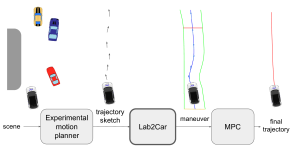
Figure 1: Lab2Car is a plug-and-play wrapper that transforms a rough trajectory sketch into spatiotemporal constraints (a maneuver). The maneuver defines an optimization problem solved by MPC to obtain a final trajectory that is safe, comfortable, and dynamically feasible. This enables rapid deployment and real-world evaluation of experimental planners that lack such properties.

To address this problem, we present Lab2Car, an optimization-based wrapper that takes a rough trajectory sketch and transforms it into a set of interpretable spatiotemporal constraints – a maneuver – which is then solved using MPC to obtain a safe, comfortable, and dynamically feasible trajectory (Fig. 1). The initial trajectory sketch captures the high-level behavioral intent, while the final trajectory captures the low-level sequence of commands that the robot must execute. This division of labor mirrors hierarchical motor control in biological brains [24] and allows for robust and safe deployment of a wide range of experimental planners.

We used Lab2Car to deploy a ML planner (Urban Driver [10]) and a search-based classical planner (A* [25, 8]) on the road. Lab2Car allowed both planners to handle a number of challenging scenarios, including adaptive cruise control (ACC), cut-ins, yielding, and maneuvering through narrow gaps. Simulations confirmed that without the safety features provided by Lab2Car, both planners would have likely caused collisions. Our contributions are as follows:

• A plug-and-play MPC-based wrapper that ensures safety, comfort, and dynamic feasibility in order to deploy arbitrary motion planners at the early stages of prototyping.

• Extensive evaluation of our approach in simulation and in the real world with two distinct types of motion planners (ML and classical).

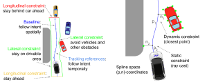
Figure 2: Anatomy of a maneuver (left) and spline-space illustration (right).

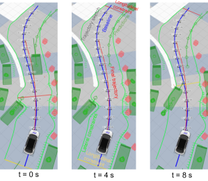
Figure 3: Lab2Car in real-world scenario. Gray arrowheads denote initial trajectory sketch from experimental planner. Spatiotemporal constraints denoted as in Fig. 2. Connected dark green circles denote predictions for other agents. Red curve denotes final 8-s open-loop trajectory from MPC.

II Maneuver definition

The input to Lab2Car is a path or trajectory sketch $\tau=\{(x_{k},y_{k},t_{k})\}_{k=0}^{K-1}$ consisting of a sequence of $K$ Cartesian waypoints $(x_{k},y_{k})$ with optional timestamps $t_{k}$. The trajectory is then converted to a maneuver: a set of spatiotemporal constraints (continuous in the spatial domain and discrete in the temporal domain) that define the feasible space of trajectories over the planning horizon (Fig. 2, left).

The baseline trajectory is modeled as a 2D quartic cardinal B-spline [26] (Fig. 2 and Fig. 3, blue curve). The spline is defined by a set of $N$ control points and corresponding knot vectors. The knot vectors are placed at spline progress values $p$ from $0$ to $N$, The spline basis functions are valid within the domain spanning from $1.5$ to $N-2.5$, ensuring that the spline is smooth and well-defined across this range.

This baseline spline serves as the reference axis of a curvilinear coordinate system which defines all subsequent trajectory constraints in terms of longitudinal (along the spline) and lateral (orthogonal to the spline) components.

Tracking references are defined as a time series $(p_{\text{ref}}(t),v_{\text{ref}}(t),a_{\text{ref}}(t))$, specifying the progress, longitudinal velocity, and longitudinal acceleration, respectively, that the AV should aim to achieve at each time point $t$ of the discretized planning horizon (Fig. 2, blue arrows). These do not apply if $\tau$ is a path (i.e., has no timestamps).

Lateral constraints are formulated as 1D spline functions extending along the baseline spline, representing the driveable space boundaries at each time point $t$ (Fig. 2 and Fig. 3, green curves). These constraints are segmented into “hard” and “soft” constraints for both the left and right boundaries of the trajectory, indexed by spline progress: $\gamma_{\text{left,hard}}(p),\gamma_{\text{left,soft}}(p),\gamma_{\text{right,hard}}(p),\gamma_{\text{right,soft}}(p)$. A separate set of lateral constraints is defined for each time point $t$ (omitted).

Longitudinal constraints are defined as a time series $(p_{\text{lower}}(t),p_{\text{upper}}(t))$ specifying the lower and upper bound on progress, respectively, at each time point $t$ of the planning horizon (Fig. 2 and Fig. 3, yellow and red lines).

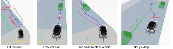
Figure 4: Lab2Car rescuing bad trajectory sketches in synthetic scenarios. Color coding as in Fig. 3

III Maneuver extraction

III-A Baseline fitting

Fitting the baseline proceeds in two steps.

Step 1: Determining spline progress: Initially, the progress value $\hat{p}_{k}$ for each waypoint point along the spline is calculated to reflect the cumulative distance along the path:

$$\hat{p}_{k}=\begin{cases}0&\text{if }k=0\\ \hat{p}_{k-1}+\frac{\|\mathbf{w}_{k-1}-\mathbf{w}_{k}\|}{\text{dist}_{\text{max}}}&\text{otherwise}\end{cases}$$ (1)

Here, $\mathbf{w}_{k}=\begin{bmatrix}x_{k},y_{k}\end{bmatrix}$ are waypoint vectors and $\text{dist}_{\text{max}}$ is the target Euclidean distance between control points on the spline.

Step 2: Control point optimization: The control points $C$ of the spline are computed using a least squares method by solving:

$$\begin{bmatrix}\mathbf{w}_{0},\mathbf{w}_{1},\dots,\mathbf{w}_{K-1},0,0,\dots,0\end{bmatrix}^{T}\approx\begin{bmatrix}B\\ \hline\cr\\ c_{reg}R\end{bmatrix}\cdot C$$ (2)

$$B_{K\times N}=\begin{bmatrix}\mathbf{b}(\hat{p}_{0}),\mathbf{b}(\hat{p}_{1}),\dots,\mathbf{b}(\hat{p}_{K-1})\end{bmatrix}^{T}$$ (3)

$$R_{N-2\times N}=\begin{bmatrix}-1&2&-1&0&\ldots\\ 0&-1&2&-1&\ldots\\ 0&0&-1&2&\ldots\\ \vdots&\vdots&\vdots&\\ \end{bmatrix},$$ (4)

where $C$ is a $N\times 2$ matrix of control points, $\mathbf{b}$ is the spline basis function, $R$ is a second-order regularization matrix which penalizes excessive curvature, and $c_{reg}$ is the regularization coefficient.

III-B Projection of dynamic obstacles onto baseline

Detections and predictions for other dynamic road entities, such as vehicles and pedestrians, are represented by time series of convex hulls subsampled to sets of $(x,y)$ points. The sampled points are then transformed into a curvilinear coordinate system aligned with the baseline, referred to as “spline-space” (Fig. 2, right). In this coordinate system, each point is expressed as $(p,n)$, where $p$ denotes progress of the closest point along the spline and $n$ represents the lateral deviation from the spline. The resulting $(p,n)$-points determine the dynamic constraints.

III-C Projection of static obstacles onto baseline

The map is represented by a raster in which each voxel is labeled as “drivable” or “non-drivable”. At uniformly sampled points along the baseline, a ray cast perpendicular to the baseline in both directions finds the nearest non-drivable voxels in the map raster (Fig. 2, right). The resulting $(p,n)$-points determine the static constraints.

Note that a similar procedure could be used for the dynamic obstacles if they were rasterized rather than vectorized.

III-D Constraint computation

Tracking references are computed by projecting each waypoint $(x_{k},y_{k})$ onto the baseline to obtain $p_{\text{ref}}(t_{k})$. Longitudinal velocity $v_{\text{ref}}(t)$ and acceleration $a_{\text{ref}}(t)$ references are approximated using finite differences.

Dynamic constraints are determined as follows:

• Dynamic obstacles farther than a certain threshold (i.e., whose closest point has $n$ greater than the threshold) impose lateral constraints only.

• Dynamic obstacles closer than the threshold can impose both lateral and longitudinal constraints, determined separately for each point based on another threshold.

Static constraints are lateral by default, unless $n$ is below a certain threshold, in which case they are longitudinal.

Stay-behind or stay-ahead: Longitudinal constraints can be imposed differently depending on the assumptions about the experimental planner. We consider two regimes:

• Stay-behind: the initial position of the AV must always fall within the longitudinal bounds. Formally, $p_{\text{lower}}(t)<p_{\text{rear}}(0)<p_{\text{front}}(0)<p_{\text{upper}}(t)\,\,\,\forall t$, where $p_{\text{rear}}(t),p_{\text{front}}(t)$ are the progress values of the rear bumper and the front bumper of the AV at time $t$, respectively. In other words, the AV always stays behind (i.e. yields for) dynamic obstacles predicted to cross its path. This is suitable for planners that output a path (i.e., no timestamps) or that do not take dynamic road actors into consideration.

• Stay-ahead: the planned position of the AV must always fall within the longitudinal bounds. Formally, $p_{\text{lower}}(t)<p_{\text{rear}}(t)<p_{\text{front}}(t)<p_{\text{upper}}(t)\,\,\,\forall t$. In this regime, the AV may stay behind or stay ahead of other actors, depending on its predicted relative position along the baseline. This is suitable for planners that output trajectories and take other road actors into consideration.

III-E Lateral constraint fitting

The lateral splines are fitted to the samples using quadratic programming [27], which maximizes the available space within the lateral constraints, subject to $\gamma_{\text{left,hard}}(p_{i})<n_{i}$ and $\gamma_{\text{right,hard}}(p_{i})>n_{i}$ for every laterally constraining sample point $(p_{i},n_{i})$. Regularization penalizes excessive curvature, ensuring smoothness of the resulting splines.

IV MPC formulation

The dynamical system is defined by the state $\mathbf{x}(t)=[p(t),n(t),\omega(t),v(t),a(t),\beta(t)]$ and the control inputs $\mathbf{u}(t)=[j(t),\Delta\beta(t)]$, where the components are:

State $\mathbf{x}(t)$
$p(t)$	Progress along the baseline
$n(t)$	Lateral error from the baseline
$\omega(t)$	Local heading relative to the baseline
$v(t)$	Longitudinal velocity
$a(t)$	Longitudinal acceleration
$\beta(t)$	Steering angle
Control $\mathbf{u}(t)$
$j(t)$	Jerk (rate of acceleration change)
$\Delta\beta(t)$	Change in steering angle

The MPC problem can be formulated as follows:

$$\min_{\mathbf{u}}\sum_{k=0}^{N-1}\ell\left(\mathbf{x}(t+k),\mathbf{u}(t+k)\right)+\ell_{f}\left(\mathbf{x}(t+N)\right)$$ (5)

subject to:

$$\mathbf{x}(t+1) =f(\mathbf{x}(t),\mathbf{u}(t))$$ (6)

$$\mathbf{C}(\mathbf{x}) \leq\mathbf{0}$$ (7)

$$\mathbf{u}_{\text{min}} \leq\mathbf{u}(t)\leq\mathbf{u}_{\text{max}}$$ (8)

$$\mathbf{x}(0) =\mathbf{x}_{0},$$ (9)

where:

• $\ell(\mathbf{x}(t+k),\mathbf{u}(t+k))$ is the non-linear stage cost function,

• $\ell_{f}(\mathbf{x}(t+N))$ is the non-linear terminal cost function,

• $N$ is the prediction horizon,

• $f(\mathbf{x}(t),\mathbf{u}(t))$ represents the state transition model – in this case, a kinematic bicycle model,

• $\mathbf{C}(\mathbf{x})$ represents the non-linear state constraints,

• $\mathbf{u}_{\text{min}},\mathbf{u}_{\text{max}}$ are the control constraints,

• $\mathbf{x}_{0}$ is the initial state.

The non-linear constraint function $\mathbf{C}(\mathbf{x})$ includes terms that ensure the footprint of the AV remains within the spline constraints throughout the planning horizon. The cost function also includes entries designed to balance various objectives, such as maintaining comfort, ensuring the AV stays within its operational boundaries, and minimizing perceived risks.

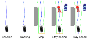
Figure 5: Lab2Car configurations (ablations).

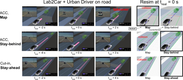
Figure 6: Lab2Car + Urban Driver on the road: sequential frames from example scenarios (rows) in different Lab2Car configurations (left) and corresponding open-loop resims (right) at the reference frame ($t_{\text{real}}=0$ s). Each row is from a unique scenario run. Resims performed with factual (bold) configuration (i.e., the one used on the road) and one counterfactual configuration. In left (on-road) panels, open-loop trajectory denoted in pink. In right (resim) panels, color coding as in Fig. 3. Resim, resimulation. See supplementary video for corresponding clips.

V Experiments

V-A Experimental planners

Machine learning: We used an open-source version of Urban Driver [28, 29], a regression-based ML planner which learns to imitate human trajectories from expert demonstrations. We trained it on lane follow and ACC scenarios from the nuPlan dataset [29]. Urban Driver takes both static and dynamic obstacles into account and outputs a trajectory with timestamps, making it suitable for deployment either in the Stay-behind or Stay-ahead configuration.

Classical planning: We used a custom implementation of A* search [25] which finds an unobstructed path to a goal pose, avoiding static obstacles and stationary vehicles. It respects road boundaries but ignores lanes, making it suitable for unstructured environments like casino pick-up/drop-off (PUDO) areas. It also ignores moving actors and only outputs a path, instead relying on Lab2Car to stay-behind other road actors.

V-B Ablations

In addition to Stay-behind and Stay-ahead, we compared several control Lab2Car configurations (Fig. 5):

• Baseline: Follow the baseline spline, ignoring waypoints and static/dynamic obstacles.

• Tracking: Track the waypoints, ignoring static/dynamic obstacles. Only applicable if $\tau$ is a trajectory with timestamps.

• Map: Track the waypoints (if applicable) and avoid static obstacles, ignoring dynamic obstacles.

V-C Simulation results

TABLE I: Closed-loop simulation results

	Safety			Comfort	Progress
Config	Coll (#) $\downarrow$	CPTO (#) $\downarrow$	Road (#) $\downarrow$	Accel (#) $\downarrow$	Dist (m) $\uparrow$
Lab2Car + Urban Driver (638 lane follow scenarios)
Baseline	0.20	0.96	0.96	2.63	193.16
Tracking	0.06	0.89	0.98	1.14	169.19
Map	0.03	0.61	0.01	0.93	164.13
Stay-behind	0.03	0.61	0.01	1.78	148.65
Stay-ahead	0.02	0.61	0.01	1.80	148.97
Lab2Car + A* (413 freespace scenarios)
Baseline	0.02	0.73	0	0.98	35.40
Stay-behind	0.01	0.43	0	0.99	26.83

Coll, front collisions. CPTO, (simulated) collision-preventative takeovers. Road, off-road violations. Accel, longitudinal acceleration violations. Dist, total distance travelled. Values averaged across scenarios.

We first evaluated closed-loop performance on 1000+ scenarios based on 30-s snippets of real-world drive logs generated by Motional AVs in Las Vegas. We used the Object Sim simulator from Applied Intuition [30], which performs realistic high-fidelity physics simulation of the entire AV stack. Since neither experimental planner provides kinematic feasibility on its own, it was necessary to perform post-processing to drive the car even in simulation. We therefore relied on Lab2Car ablations as trajectory smoothers to obtain baselines approximating the unconstrained planners.

Lab2Car + Urban Driver was evaluated on 638 lane follow and ACC scenarios (Tab. I, top). Tracking the ML trajectory had fewer collisions and simulated takeovers than simply following the baseline, indicating that Urban Driver had learned to avoid other actors. However, it had trouble staying on the road, which was improved substantially when Map constraints were additionally imposed. Constraining Urban Driver to stay-behind or stay-ahead of other actors further reduced collisions. However, this came at the expense of comfort and progress, likely due to the extra braking.

Lab2Car + A* was evaluated on 413 PUDO scenarios (Tab. I, bottom). Following the baseline performed surprisingly well, likely because most actors in PUDO areas are stationary and the planner avoids them by design. Constraining it to stay-behind moving actors further improved safety.

V-D Real-world driving

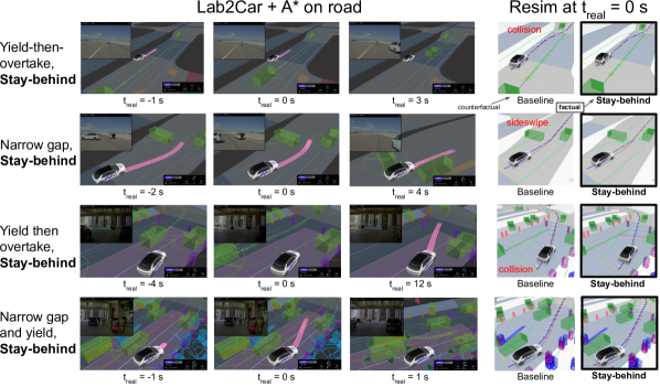
Figure 7: Lab2Car + A* on the road: private track (top two rows) and public road (bottom two rows). Notation as in Fig. 6.

We deployed both planners using with Lab2Car on Motional IONIQ 5 self-driving cars in Las Vegas. Perception, prediction [31], and mapping inputs were provided by the corresponding modules of the Motional AV stack. All drive tests were conducted with an experienced safety driver ready to take over in case of unsafe behavior and in situations outside of the operationally defined domain of the planners. Representative scenarios are included in the supplementary video.

TABLE II: On-road results

	Safety	Comfort	Progress
Config	CPTO (#)	Accel (#)	Dist (m)	Time (s)
Lab2Car + Urban Driver (private track)
Map	2	7	264.4	75
Stay-behind	0	27	1327.0	378
Stay-ahead	0	45	1834.1	638
Lab2Car + A* (private track)
Stay-behind	0	4	772.4	567
Lab2Car + A* (public road)
Stay-behind	0	6	641.3	7022

Abbreviations as in Tab. I, except CPTO stands for actual takeovers. Values totaled for each configuration.

Lab2Car + Urban Driver on private track: We staged 8 ACC and 9 cut-in scenarios on a private test track (Tab. II, top). As a baseline, we used the Map configuration, which resulted in two safety-related takeovers as the planner failed to stop for the vehicle ahead (Fig. 6, top row). Resimulations (resims) confirmed that the ML trajectory would have indeed resulted in a collision, which the Stay-behind configuration would have prevented (Fig. 6, top right). Accordingly, repeating the scenarios in the Stay-behind configuration resulted in safe stopping behind the lead vehicle (Fig. 6, middle row). Performance was similar using the Stay-ahead configuration (Fig. 6, bottom row). Overall, the planner slowed and/or stopped successfully for 6/8 ACC and 9/9 cut-in scenarios.

While more sophisticated Lab2Car configurations corrected the unsafe behavior of Urban Driver, the planner repeatedly got stuck outputting stationary trajectories after stopping, for reasons unrelated to Lab2Car. We therefore chose not to deploy Lab2Car + Urban Driver on public roads.

Lab2Car + A* on private track: We similarly staged 4 overtake, 5 yield-then-overtake, and 9 narrow gap scenarios using the Stay-behind configuration (Tab. II, middle; Fig. 7, top two rows). The planner performed successfully in all scenarios, with the exception of getting stuck in one narrow gap scenario. There were no safety-related takeovers.

Lab2Car + A* on public roads: After rigorously evaluating Lab2Car + A* in simulation and on the private test track, we deployed it on the Las Vegas strip. The experimental planner was geofenced to casino PUDO areas – dense, unstructured environments with pedestrians, slowly moving and parked vehicles, traffic cones, and obstacles. It was deployed as part of a larger planning system that included an additional lane-based planner and a selection mechanism for arbitrating between the two. We only report results for periods when Lab2Car + A* was driving the AV.

On public roads, Lab2Car + A* showed performance similar to the private test track (Tab. II, bottom; Fig. 7, bottom two rows). It handled scenarios with multiple lane changes, jaywalking pedestrians, and multiple passing vehicles (see supplementary video). There were no safety-related takeovers.

VI Conclusion

In this work, we introduced Lab2Car, an optimization-based method for safely deploying experimental planners in real self-driving cars. We demonstrated the versatility of our approach by using it to deploy a ML-based planner and a classical search-based planner, neither of which could provide safety, comfort, or even kinematic feasibility on its own. Results from large-scale closed-loop simulations showed that Lab2Car can improve safety and comfort, while adhering to the original intent of the experimental planner.

Deploying on the private test track substantiated these findings and also gave us early indication of deficiencies in the ML-based planner, while providing assurance of the behavior of the search-based planner. Ultimately, Lab2Car allowed us to deploy the relatively simple search-based planner on public roads in Las Vegas, where it successfully handled challenging scenarios in complex environments, such as navigating through narrow gaps between vehicles while avoiding pedestrians in crowded PUDO areas.

Lab2Car streamlines the path from incubating an idea in the lab to testing it on the car, offering early insights into the real-world performance of experimental planners at the initial stages of prototyping. This can allow researchers in academia and industry to focus on promising ideas and rule out dead ends before investing too much effort in polishing them. We believe this can dramatically accelerate progress towards resolving the planning bottleneck in autonomous driving and making a driverless future for all a reality.

Supplementary Material

Here we provide additional background and details about how Lab2Car works and how it was evaluated.

VII Related works

VII-A Classical planning

Classical approaches treat the planning problem as graph search [8, 9] or an optimization problem [9]. Examples include A* [32], RRT [33, 9], PRM* [34], dynamic programming [35], MPCC [36]. Since the objective function is often hand-designed, parameter tuning is a painstaking process and generalization is often poor. As result, classical planners are often confined to very simple domains (e.g., lane follow [37]).

To ensure feasible trajectories, classical planners often incorporate vehicle dynamics models in the transition function (e.g., a bicycle model [38]). Safety and comfort are often achieved via the objective function. For graph search, this is often computed locally at each transition [34, 38], pruning bad states on-the-fly. Optimization-based approaches frame motion planning as a constrained optimization problem that is often solved using MPC, which can solve jointly for safety, comfort, and feasibility [39, 40]. Hybrid approaches combine the two techniques, e.g. using graph search to get a coarse-level path and MPC to optimize the local state transitions [41]. Control barrier functions (CBFs) have been widely used as an alternative to MPC to ensure safety efficiently [42, 43, 44]. Crucially, for classical planners, safety, comfort, and feasibility are often uniquely intertwined with the motion planning logic, resulting in bespoke planning systems that cannot be readily unbundled to benefit the deployment of less sophisticated experimental planners.

VII-B Learning-based planning

Learning-based (or ML-based) approaches attempt to learn a driving policy from real or simulated data. Examples include imitation learning [45, 12, 46, 47, 10], reinforcement learning [48, 49, 50, 51, 52], inverse reinforcement learning [53, 54, 11], and combinations thereof [55]. Recently, these approaches have been boosted techniques from generative AI [56, 57, 58, 59, 60, 61]. However, pure ML planning often cannot guarantee safety, comfort, or even basic dynamic feasibility, necessitating additional layers that often originate in classical planning.

One approach is to restrict the solution space to a discrete set of trajectories generated to satisfy the desired constraints using hand-engineered rules [4]. DriveIRL [11] uses classification to select from a set of kinematically feasible trajectories that follow the lane and do not lead to unavoidable collisions. SafetyNet [17] infers a single trajectory which is projected onto a set of feasible lane fallow trajectories. While this approach has facilitated real-world deployment of ML planners like DriveIRL and SafetyNet, it does not scale to complex scenarios, such as navigation in unstructured environments, as the trajectory space becomes intractably large.

Alternatively, ML can be used to approximate different components of classical planners, such is the value function in MCTS [62, 63] or the transition function in MPC [64]. More commonly, classical optimization techniques such as a PID controller [19, 20] or MPC [21] are used post-process the output of a ML planner. Most relevant to our work, DiffStack [22] and DIPP [23] include a differential MPC as the final layer of a neural AV stack. In addition to ensuring feasibility, safety, and comfort, this allows for the parameters of the entire AV stack it to be learned end-to-end. However, this comes at the cost of increased complexity and tight coupling between the MPC and the planning module, making the MPC less portable to other planners, especially if they are not ML-based. Furthermore, to ensure differentiability, the MPC cost function needs to be smooth, which makes it challenging to impose hard constraints, such as staying on the road or avoiding collisions. This can weaken the safety guarantees, while potentially introducing undesirable side effects, such as unnecessarily nudging the AV away from obstacles. Notably, to the best of our knowledge, neither approach has been used for real-world deployment.

VIII Maneuver extraction

A flowchart illustrating maneuver extraction is shown in Fig. 8.

Figure 8: Lab2Car maneuver extraction flow diagram.

VIII-A Spline-space conversion

Cartesian points are projected onto the spline by finding the closest point. This is performed iteratively for each point by approximating the spline locally as a circle and then finding the closest point of the circle to the query point (Alg. 1).

Algorithm 1 Iterative closest point search on spline

1:Input: Spline $spline$, Query Point $q_{p}$

2:Output: Closest Point on Spline

3:$sampled\_points\leftarrow\text{SamplePoints}(spline,num\_samples)$

4:$closest_{p}\leftarrow\text{argmin}_{p}\;\text{EuclideanDistance}(sampled\_points,q_{p})$

5:for $i=1$ to $3$ do

6:    $center,radius\leftarrow\text{ApproximateAsCircle}(spline,closest_{p})$

7:    $delta_{p}\leftarrow\text{ComputeDelta}(center,radius,q_{p},spline,closest_{p})$

8:    $closest_{p}\leftarrow closest_{p}+delta_{p}$

9:end for

10:return $spline(closest_{p})$

VIII-B Lateral constraint fitting

The cost function additionally incorporates a regularization matrix $R$, which governs the rate of change of the spline. This regularization is represented by:

$$R=\begin{bmatrix}-1&1&0&0&\ldots\\ 0&-1&1&0&\ldots\\ 0&0&-1&1&\ldots\\ \vdots&\vdots&\vdots&\\ \end{bmatrix}$$ (10)

This matrix serves to smooth transitions and maintain a consistent gradient across the spline, aiding in the stabilization of the fitted trajectory. This approach ensures that the spline tubes accurately reflect the spatial constraints imposed by the surrounding environment.

IX MPC formulation

The MPC non-linear constraint function is given by:

$$\mathbf{C(x)}=\begin{bmatrix}0.5\cdot\mathbf{W}+\mathbf{FL}\cdot\sin(\omega)-\gamma_{\text{left}}(p+\mathbf{FL}\cdot\cos(\omega))\\ 0.5\cdot\mathbf{W}+\mathbf{FL}\cdot\sin(\omega)+\gamma_{\text{right}}(p+\mathbf{FL}\cdot\cos(\omega))\\ 0.5\cdot\mathbf{W}-\mathbf{RL}\cdot\sin(\omega)-\gamma_{\text{left}}(p+\mathbf{RL}\cdot\cos(\omega))\\ 0.5\cdot\mathbf{W}-\mathbf{RL}\cdot\sin(\omega)+\gamma_{\text{right}}(p+\mathbf{RL}\cdot\cos(\omega))\\ \vdots\end{bmatrix}$$ (11)

X Experiments

X-A Experimental planners

We evaluated Lab2Car together with two motion planners that cover two main types of approaches used in the literature and industry: ML and search.

X-A1 ML-based planner – Urban Driver

We used Urban Driver [10], a ML-based motion planner which uses regression to learn to imitate an expert driver using closed-loop rollouts. We adapted the open-source version of Urban Driver made public by the authors and trained it on the nuPlan dataset [28, 29] [https://github.com/motional/nuplan-devkit/]. We restricted the training set to lane follow and ACC scenarios. The input to the model was a vectorized map and a vectorized representation of the other agents in the scene (vehicles, pedestrians, bicyclists, etc.) relative to the AV. The output was a sequence of 16 $(x,y)$-waypoints corresponding to an 8-s open-loop AV trajectory at 2 Hz. We trained the model with multistep training: for each scenario, we rolled out the model for 13 s at 2 Hz and supervised the output open-loop trajectory at each time step with the corresponding ground truth expert trajectory using an L2 loss.

X-A2 Search-based planner – A*

We used A* [25], a classical graph search algorithm which we adapted for freespace motion planning. Vertices were defined by a discrete space of $(x,y,\theta)$-poses and edges were defined by feasible transitions between poses, with weights representing the relative cost of motion. The heuristic was an (approximate) lower bound of the cost-to-go to the target. The input to the planner was a starting pose, a target pose, and an occupancy grid with the drivable area and the static agents. The output was a sequence of $(x,y,\theta)$-waypoints connecting the starting pose to the target pose. The waypoints did not have corresponding timestamps, so unlike Urban Driver, the output corresponded to a purely spatial path with no temporal dimension. This planner was designed for freespace planning in unstructured environments (e.g., parking lots) and ignored dynamic agents, instead relying on Lab2Car for active collision avoidance.

X-B Perception, Prediction, and Mapping

For simulated scenarios, object-oriented representations of the scene from the simulator were fed to the motion planner and to Motional’s in-house prediction module [31], which generated unimodal 8-s predictions for each actor in the scene at each iteration of the simulation. These predictions were used by Lab2Car to compute lateral and longitudinal constraints for each open-loop time step of the maneuver. For real-world driving, we similarly used Motional’s in-house perception system to recreate an object-oriented representation of the scene from camera and lidar sensor data. Perception ran at 20 Hz, while prediction ran at 10 Hz, at the same rate as planning. We also assume access to a high-definition map. While robust perception, prediction, and mapping are critical for both motion planners and for Lab2Car, they are also integral components of a modular AV stack and are widely used in industry. Therefore we omit their details as they fall beyond the scope of this paper.

X-C Scenarios

We evaluated Lab2Car using the Object Sim simulator (formerly Simian) from Applied Intuition [30] on 1000+ closed-loop resim scenarios based on real-world drive logs generated by Motional AVs in Las Vegas. Each scenario consisted of a 30-s snippet from the drive log downsampled to 10 Hz. The first 3 s of each scenario consisted of a “warm-up” period during which the system was run in open loop but its inputs and outputs were clamped to (i.e., replayed from) the log. For the remaining 27 s, the system was run in closed loop at 10 Hz. The open-loop trajectory from each iteration was tracked by a VDS controller, which was designed to mimic the dynamics of the real AV. All other actors were replayed from the log, i.e. they were nonreactive to any deviations of AV behavior resulting from the closed-loop simulation.

Given the complementary strengths of the two motion planners, we evaluated them on different sets of scenarios:

X-C1 Nominal Scenarios

We evaluated Lab2Car + Urban Driver on 638 nominal lane follow and ACC scenarios on the Las Vegas Strip similar to those from the nuPlan training set. They were meant to illustrate how Lab2Car can act as a rule-based safety wrapper and smoother for a well-trained but imperfect ML planner.

X-C2 Freespace Scenarios

We evaluated Lab2Car + A* on 413 scenarios from pick-up/drop-off (PuDo) areas of multiple casinos off the Las Vegas Strip. The unstructured PuDo environments included irregularly parked cars, slow-moving traffic, pedestrians jaywalking and getting on and off of vehicles. They were meant to demonstrate how Lab2Car can be used in conjunction with a purely spatial planner to allow progress while ensuring safety in unstructured environments.

X-D Metrics

To illustrate how Lab2Car impacts safety, comfort, and progress, we calculated the following metrics:

• Front collisions (Coll): instances when the AV collided with a vehicle in front of it.

• Collision-preventative takeovers (CPTO): for real-world driving, instances when the safety driver took over to prevent a collision. For simulations, instances when the AV produced unsafe behavior that would have plausibly led to a CPTO. This includes any collision, drivable area violation, nearest actor violation (min. clearance $<$ 0.15 m to any bicycle/vehicle/obstacle), or proximity speed violation (min. clearance $<$ 0.25 m and AV max. speed $>$ 5.0 m/s for vehicles or $>$ 0.0 m/s for bicycles/pedestrians).

• Off-road (Road): instances when any point of the AV footprint was outside the driveable area.

• Acceleration violation (Accel): instances when the (absolute) longitudinal acceleration was above a certain threshold. When decelerating, the threshold was 2.5 m/s² for speeds $<$ 10 m/s and 1.5 m/s² for speeds $>$ 20 m/s, with linear interpolation for in-between speeds. When accelerating, the threshold was 2.0 m/s² for speeds $<$ 10 m/s and 1.0 m/s² for speeds $>$ 15 m/s, with linear interpolation for in-between speeds.

• Distance traveled (Dist): total distance traveled by the AV for the entire duration of the scenario.

For simulations, metrics were calculated separately for each scenario based on the closed-loop trajectory of the AV and the replayed trajectories of the other actors along the entire duration of the scenario. We aggregated each metric across scenarios by averaging for each configuration.

For real-world driving, metrics were computed separately for each run with a given planner and Lab2Car configuration.

X-E Ablations

To study the relative importance of different Lab2Car components, we evaluated different ablated versions (configurations) of Lab2Car (Fig. 5). We present them here in order from simplest to most complex, with each subsequent configuration enabling a superset of the components enabled in the previous configuration:

• Baseline: We only fitted the baseline spline to the initial trajectory sketch. No lateral or longitudinal constraints were imposed based on the map or other actors in the scene. No tracking costs were imposed and the AV was allowed to accelerate to the speed limit. In this configuration, the system simply generates dynamically feasible trajectories that follow the spatial (but not the temporal) intent of the initial trajectory sketch.

• Tracking: In addition to fitting the baseline (as in the Baseline configuration), longitudinal tracking costs were imposed at waypoint projections onto the baseline. These encouraged the AV to reach the corresponding speed derived from the initial directory sketch at each corresponding waypoint. No lateral or longitudinal constraints were imposed. In this configuration, the system tracks the intent of the initial trajectory sketch both spatially and temporally.

• Map: In addition to fitting the baseline and tracking the waypoints (as in the Tracking configuration), constraints were imposed based on the map. Specifically, the lateral tube was restricted to the boundaries of the drivable area. If the width of the lateral tube shrunk below a certain threshold (2 m), indicating that the AV will surely violate the lateral bounds and drive off the road, a longitudinal constraint was imposed. In this configuration, the system tracks the intent of the initial trajectory sketch, while remaining on the drivable area.

• Stay-behind: In addition to fitting the baseline, tracking the waypoints, and staying on the drivable area (as in the Map configuration), constraints were imposed based on the other actors in the scene. Specifically, lateral constraints were imposed on actors within 4 m of the baseline, to ensure the AV circumvents them. If an actor was too close to the baseline ($<$ 2 m), indicating that driving around them is unsafe or infeasible, a stay-behind longitudinal constraint was imposed. In this configuration, the AV was constrained to always stay behind other actors crossing its path and pass after they have moved out of the way.

• Stay-ahead: This included all components from the Stay-behind configuration, namely fitting the baseline, tracking the waypoints, staying on the drivable area, and constraints based on the other actors. However, the longitudinal constraints were computed based on where the AV was expected to be along the baseline, according to the waypoint projections. Specifically, if the AV was expected to be behind an actor at time $t$, a stay-behind longitudinal constraint was imposed to ensure that AV indeed remains behind at time $t$, as in the Stay-behind configuration. However, if the AV was expected to be in front of the actor at time $t$, a stay-ahead longitudinal constraint was imposed instead, ensuring that AV passes the actor by time $t$. Thus the AV could either stay behind or stay ahead other actors crossing its path, allowing for a diverse set of behaviors, including lane merging and cut-ins.

In stimulation, we evaluated Urban Driver in all configurations. For A*, we only used the Baseline and Stay-behind configurations. Since our A* implementation produces a path rather than a trajectory, there are no timestamps associated with the waypoints, so tracking references and stay-ahead constraints could not be computed. Additionally, since the occupancy grid a priori constrains the search to only consider poses on the driveable area, the Map configuration produced identical performance to the Baseline configuration.

On the road, we evaluated Urban Driver in the Map, Stay-behind, and Stay-ahead configurations, given the relatively poor performance of the Baseline and Tracking configurations in simulation.

References

- [1] Y. Zhou and O. Tuzel, “Voxelnet: End-to-end learning for point cloud based 3d object detection,” in Proceedings of the IEEE Conference on Computer Vision and Pattern Recognition (CVPR), June 2018, pp. 4490–4499.
- [2] A. H. Lang, S. Vora, H. Caesar, L. Zhou, J. Yang, and O. Beijbom, “Pointpillars: Fast encoders for object detection from point clouds,” in Proceedings of the IEEE Conference on Computer Vision and Pattern Recognition (CVPR), June 2019, pp. 12 697–12 705.
- [3] S. Vora, A. H. Lang, B. Helou, and O. Beijbom, “Pointpainting: Sequential fusion for 3d object detection,” in Proceedings of the IEEE/CVF Conference on Computer Vision and Pattern Recognition (CVPR), June 2020, pp. 4604–4612.
- [4] T. Phan-Minh, E. C. Grigore, F. A. Boulton, O. Beijbom, and E. M. Wolff, “Covernet: Multimodal behavior prediction using trajectory sets,” in Proceedings of the IEEE/CVF Conference on Computer Vision and Pattern Recognition (CVPR), 2020, pp. 14 074–14 083.
- [5] T. Yin, X. Zhou, and P. Krahenbuhl, “Center-based 3d object detection and tracking,” in Proceedings of the IEEE/CVF Conference on Computer Vision and Pattern Recognition (CVPR), 2021, pp. 11 784–11 793.
- [6] Q. Chen, S. Vora, and O. Beijbom, “Polarstream: Streaming object detection and segmentation with polar pillars,” in Proceedings of the 34th Conference on Neural Information Processing Systems (NeurIPS), 2021.
- [7] M. Liang, B. Yang, R. Hu, Y. Chen, R. Liao, S. Feng, and R. Urtasun, “Learning lane graph representations for motion forecasting,” in Proceedings of the European Conference on Computer Vision (ECCV), 2020, pp. 541–556.
- [8] S. M. LaValle, Planning algorithms. Cambridge university press, 2006.
- [9] B. Paden, M. Čáp, S. Z. Yong, D. Yershov, and E. Frazzoli, “A survey of motion planning and control techniques for self-driving urban vehicles,” IEEE Transactions on Intelligent Vehicles, vol. 1, no. 1, pp. 33–55, 2016.
- [10] O. Scheel, L. Bergamini, M. Wolczyk, B. Osiński, and P. Ondruska, “Urban driver: Learning to drive from real-world demonstrations using policy gradients,” in Conference on Robot Learning. PMLR, 2022, pp. 718–728.
- [11] T. Phan-Minh, F. Howington, T.-S. Chu, M. S. Tomov, R. E. Beaudoin, S. U. Lee, N. Li, C. Dicle, S. Findler, F. Suarez-Ruiz et al., “Driveirl: Drive in real life with inverse reinforcement learning,” in 2023 IEEE International Conference on Robotics and Automation (ICRA). IEEE, 2023, pp. 1544–1550.
- [12] M. Bojarski, D. Del Testa, D. Dworakowski, B. Firner, B. Flepp, P. Goyal, L. D. Jackel, M. Monfort, U. Muller, J. Zhang et al., “End to end learning for self-driving cars,” arXiv preprint arXiv:1604.07316, 2016.
- [13] F. Codevilla, E. Santana, A. M. Lopez, and A. Gaidon, “Exploring the limitations of behavior cloning for autonomous driving,” in Proceedings of the IEEE/CVF International Conference on Computer Vision (ICCV), October 2019, pp. 9329–9338.
- [14] M. Bansal, A. Krizhevsky, and A. Ogale, “Chauffeurnet: Learning to drive by imitating the best and synthesizing the worst,” in Proceedings of Robotics: Science and Systems (RSS), 2019.
- [15] W. Zeng, W. Luo, S. Suo, A. Sadat, B. Yang, S. Casas, and R. Urtasun, “End-to-end interpretable neural motion planner,” in Proceedings of the IEEE/CVF Conference on Computer Vision and Pattern Recognition (CVPR), 2019.
- [16] J. Hawke, R. Shen, C. Gurau, S. Sharma, D. Reda, N. Nikolov, P. Mazur, S. Micklethwaite, N. Griffiths, A. Shah et al., “Urban driving with conditional imitation learning,” in Proceedings of the IEEE International Conference on Robotics and Automation (ICRA), 2020.
- [17] M. Vitelli, Y. Chang, Y. Ye, A. Ferreira, M. Wołczyk, B. Osiński, M. Niendorf, H. Grimmett, Q. Huang, A. Jain et al., “Safetynet: Safe planning for real-world self-driving vehicles using machine-learned policies,” in Proceedings of the IEEE International Conference on Robotics and Automation (ICRA), 2022.
- [18] Y. Hu, J. Yang, L. Chen, K. Li, C. Sima, X. Zhu, S. Chai, S. Du, T. Lin, W. Wang et al., “Planning-oriented autonomous driving,” in Proceedings of the IEEE/CVF Conference on Computer Vision and Pattern Recognition (CVPR), 2023.
- [19] J. Chen, B. Yuan, and M. Tomizuka, “Deep imitation learning for autonomous driving in generic urban scenarios with enhanced safety,” in 2019 IEEE/RSJ International Conference on Intelligent Robots and Systems (IROS), 2019, pp. 2884–2890.
- [20] K. B. Naveed, Z. Qiao, and J. M. Dolan, “Trajectory planning for autonomous vehicles using hierarchical reinforcement learning,” in 2021 IEEE International Intelligent Transportation Systems Conference (ITSC), 2021, pp. 601–606.
- [21] K. P. Wabersich and M. N. Zeilinger, “A predictive safety filter for learning-based control of constrained nonlinear dynamical systems,” Automatica, vol. 129, p. 109597, 2021.
- [22] P. Karkus, B. Ivanovic, S. Mannor, and M. Pavone, “Diffstack: A differentiable and modular control stack for autonomous vehicles,” in Proceedings of The 6th Conference on Robot Learning, 2023, pp. 2170–2180.
- [23] Z. Huang, H. Liu, J. Wu, and C. Lv, “Differentiable integrated motion prediction and planning with learnable cost function for autonomous driving,” IEEE Transactions on Neural Networks and Learning Systems, pp. 1–15, 2023.
- [24] J. Merel, M. Botvinick, and G. Wayne, “Hierarchical motor control in mammals and machines,” Nature communications, vol. 10, no. 1, pp. 1–12, 2019.
- [25] P. E. Hart, N. J. Nilsson, and B. Raphael, “A formal basis for the heuristic determination of minimum cost paths,” IEEE transactions on Systems Science and Cybernetics, vol. 4, no. 2, pp. 100–107, 1968.
- [26] L. Piegl and W. Tiller, The NURBS book. Springer Science & Business Media, 2012.
- [27] S. J. Wright, “Numerical optimization,” 2006.
- [28] H. Caesar, J. Kabzan, K. S. Tan, W. K. Fong, E. Wolff, A. Lang, L. Fletcher, O. Beijbom, and S. Omari, “nuplan: A closed-loop ml-based planning benchmark for autonomous vehicles,” arXiv preprint arXiv:2106.11810, 2021.
- [29] N. Karnchanachari, D. Geromichalos, K. S. Tan, N. Li, C. Eriksen, S. Yaghoubi, N. Mehdipour, G. Bernasconi, W. K. Fong, Y. Guo, and H. Caesar, “Towards learning-based planning: The nuplan benchmark for real-world autonomous driving,” in 2024 IEEE International Conference on Robotics and Automation (ICRA), 2024, pp. 629–636.
- [30] “Applied Intuition Object Sim,” https://www.appliedintuition.com/products/object-sim, accessed: 2024-05-12.
- [31] S. Afshar, N. Deo, A. Bhagat, T. Chakraborty, Y. Shao, B. R. Buddharaju, A. Deshpande, and H. Cui, “Pbp: Path-based trajectory prediction for autonomous driving,” arXiv preprint arXiv:2309.03750, 2023.
- [32] J. Ziegler, M. Werling, and J. Schroder, “Navigating car-like robots in unstructured environments using an obstacle sensitive cost function,” in Proceedings of the IEEE Intelligent Vehicles Symposium, 2008, pp. 787–791.
- [33] J. J. Kuffner Jr and S. M. Lavalle, “Rrt-connect: An efficient approach to single-query path planning,” in Proceedings of the IEEE International Conference on Robotics and Automation (ICRA), 2000, pp. 995–1001.
- [34] S. Karaman and E. Frazzoli, “Sampling-based algorithms for optimal motion planning,” The international journal of robotics research, vol. 30, no. 7, pp. 846–894, 2011.
- [35] M. Montemerlo, J. Becker, S. Bhat, H. Dahlkamp, D. Dolgov, S. Ettinger, D. Haehnel, T. Hilden, G. Hoffmann, B. Huhnke, D. Johnston, S. Klumpp, D. Langer, A. Levandowski, J. Levinson, J. Marcil, D. Orenstein, J. Paefgen, I. Penny, A. Petrovskaya, M. Pflueger, G. Stanek, D. Stavens, A. Vogt, and S. Thrun, “Junior: The stanford entry in the urban challenge,” in Journal of Field Robotics, 2009, pp. 569–597.
- [36] L. Ferranti, B. Brito, E. Pool, Y. Zheng, R. M. Ensing, R. Happee, B. Shyrokau, J. F. Kooij, J. Alonso-Mora, and D. M. Gavrila, “Safevru: A research platform for the interaction of self-driving vehicles with vulnerable road users,” in 2019 IEEE Intelligent Vehicles Symposium (IV). IEEE, 2019, pp. 1660–1666.
- [37] M. Treiber, A. Hennecke, and D. Helbing, “Congested traffic states in empirical observations and microscopic simulations,” Physical review E, vol. 62, no. 2, p. 1805, 2000.
- [38] M. McNaughton, C. Urmson, J. M. Dolan, and J.-W. Lee, “Motion planning for autonomous driving with a conformal spatiotemporal lattice,” in 2011 IEEE International Conference on Robotics and Automation. IEEE, 2011, pp. 4889–4895.
- [39] F. Borrelli, P. Falcone, T. Keviczky, J. Asgari, and D. Hrovat, “Mpc-based approach to active steering for autonomous vehicle systems,” International journal of vehicle autonomous systems, vol. 3, no. 2-4, pp. 265–291, 2005.
- [40] C. Urmson, J. Anhalt, D. Bagnell, C. Baker, R. Bittner, M. Clark, J. Dolan, D. Duggins, T. Galatali, C. Geyer et al., “Autonomous driving in urban environments: Boss and the urban challenge,” Journal of field Robotics, vol. 25, no. 8, pp. 425–466, 2008.
- [41] L. Li, Y. Miao, A. H. Qureshi, and M. C. Yip, “Mpc-mpnet: Model-predictive motion planning networks for fast, near-optimal planning under kinodynamic constraints,” IEEE Robotics and Automation Letters, vol. 6, no. 3, pp. 4496–4503, 2021.
- [42] A. D. Ames, S. Coogan, M. Egerstedt, G. Notomista, K. Sreenath, and P. Tabuada, “Control barrier functions: Theory and applications,” in 2019 18th European control conference (ECC). IEEE, 2019, pp. 3420–3431.
- [43] G. Notomista, M. Wang, M. Schwager, and M. Egerstedt, “Enhancing game-theoretic autonomous car racing using control barrier functions,” in 2020 IEEE International Conference on Robotics and Automation (ICRA), 2020, pp. 5393–5399.
- [44] J. Seo, J. Lee, E. Baek, R. Horowitz, and J. Choi, “Safety-critical control with nonaffine control inputs via a relaxed control barrier function for an autonomous vehicle,” IEEE Robotics and Automation Letters, vol. 7, no. 2, pp. 1944–1951, 2022.
- [45] D. A. Pomerleau, “Alvinn: An autonomous land vehicle in a neural network,” in Advances in Neural Information Processing Systems (NIPS), vol. 1, 1988, pp. 305–313. [Online]. Available: https://proceedings.neurips.cc/paper/1988/file/812b4ba287f5ee0bc9d43bbf5bbe87fb-Paper.pdf
- [46] M. Bansal, A. Krizhevsky, and A. Ogale, “Chauffeurnet: Learning to drive by imitating the best and synthesizing the worst,” in Proceedings of Robotics: Science and Systems (RSS), 2018.
- [47] A. Kendall, J. Hawke, D. Janz, P. Mazur, D. Reda, J.-M. Allen, V.-D. Lam, A. Bewley, and A. Shah, “Learning to drive in a day,” in 2019 international conference on robotics and automation (ICRA). IEEE, 2019, pp. 8248–8254.
- [48] A. Dosovitskiy, G. Ros, F. Codevilla, A. Lopez, and V. Koltun, “Carla: An open urban driving simulator,” in Proceedings of the 1st Annual Conference on Robot Learning, vol. 78. PMLR, 2017, pp. 1–16. [Online]. Available: https://proceedings.mlr.press/v78/dosovitskiy17a.html
- [49] M. Riedmiller, M. Montemerlo, and H. Dahlkamp, “Learning to drive a real car in 20 minutes,” in 2007 Frontiers in the Convergence of Bioscience and Information Technologies. IEEE, 2007, pp. 645–650.
- [50] A. Kendall, J. Hawke, D. Janz, P. Mazur, D. Reda, J.-M. Allen, V.-D. Lam, A. Bewley, and A. Shah, “Learning to drive in a day,” in Proceedings of the 2019 International Conference on Robotics and Automation (ICRA). IEEE, 2019, pp. 8248–8254.
- [51] D. Chen, B. Zhou, V. Koltun, and P. Krähenbühl, “Learning by cheating,” in Proceedings of the Conference on Robot Learning. PMLR, 2020, pp. 66–75. [Online]. Available: https://proceedings.mlr.press/v155/chen21b.html
- [52] D. Chen, V. Koltun, and P. Krähenbühl, “Learning to drive from a world on rails,” in Proceedings of the IEEE/CVF International Conference on Computer Vision (ICCV), 2021, pp. 15 590–15 599. [Online]. Available: https://openaccess.thecvf.com/content/ICCV2021/html/Chen_Learning_to_Drive_From_a_World_on_Rails_ICCV_2021_paper.html
- [53] P. Abbeel and A. Y. Ng, “Apprenticeship learning via inverse reinforcement learning,” in Proceedings of the Twenty-First International Conference on Machine Learning (ICML). ACM, 2004, pp. 1–8.
- [54] Z. Huang, J. Wu, and C. Lv, “Driving behavior modeling using naturalistic human driving data with inverse reinforcement learning,” IEEE Transactions on Intelligent Transportation Systems, pp. 1–13, 2021.
- [55] Y. Lu, J. Fu, G. Tucker, X. Pan, E. Bronstein, R. Roelofs, B. Sapp, B. White, A. Faust, S. Whiteson et al., “Imitation is not enough: Robustifying imitation with reinforcement learning for challenging driving scenarios,” in 2023 IEEE/RSJ International Conference on Intelligent Robots and Systems (IROS). IEEE, 2023, pp. 7553–7560.
- [56] J. Mao, Y. Qian, H. Zhao, and Y. Wang, “Gpt-driver: Learning to drive with gpt,” arXiv preprint arXiv:2310.01415, 2023.
- [57] S. Huang, Z. Wang, P. Li, B. Jia, T. Liu, Y. Zhu, W. Liang, and S.-C. Zhu, “Diffusion-based generation, optimization, and planning in 3d scenes,” in Proceedings of the IEEE/CVF Conference on Computer Vision and Pattern Recognition, 2023, pp. 16 750–16 761.
- [58] A. Seff, B. Cera, D. Chen, M. Ng, A. Zhou, N. Nayakanti, K. S. Refaat, R. Al-Rfou, and B. Sapp, “Motionlm: Multi-agent motion forecasting as language modeling,” in Proceedings of the IEEE/CVF International Conference on Computer Vision, 2023, pp. 8579–8590.
- [59] S. Wang, Z. Yu, X. Jiang, S. Lan, M. Shi, N. Chang, J. Kautz, Y. Li, and J. M. Alvarez, “Omnidrive: A holistic llm-agent framework for autonomous driving with 3d perception, reasoning and planning,” arXiv preprint arXiv:2405.01533, 2024.
- [60] Z. Xu, Y. Zhang, E. Xie, Z. Zhao, Y. Guo, K.-Y. K. Wong, Z. Li, and H. Zhao, “Drivegpt4: Interpretable end-to-end autonomous driving via large language model,” IEEE Robotics and Automation Letters, 2024.
- [61] C. Pan, B. Yaman, T. Nesti, A. Mallik, A. G. Allievi, S. Velipasalar, and L. Ren, “Vlp: Vision language planning for autonomous driving,” in Proceedings of the IEEE/CVF Conference on Computer Vision and Pattern Recognition, 2024, pp. 14 760–14 769.
- [62] C.-J. Hoel, K. Driggs-Campbell, K. Wolff, L. Laine, and M. J. Kochenderfer, “Combining planning and deep reinforcement learning in tactical decision making for autonomous driving,” IEEE transactions on intelligent vehicles, vol. 5, no. 2, pp. 294–305, 2019.
- [63] R. Chekroun, T. Gilles, M. Toromanoff, S. Hornauer, and F. Moutarde, “Mbappe: Mcts-built-around prediction for planning explicitly,” in 2024 IEEE Intelligent Vehicles Symposium (IV). IEEE, 2024, pp. 2062–2069.
- [64] M. Rokonuzzaman, N. Mohajer, S. Nahavandi, and S. Mohamed, “Model predictive control with learned vehicle dynamics for autonomous vehicle path tracking,” IEEE Access, vol. 9, pp. 128 233–128 249, 2021.