How Combined Pairwise and Higher-Order Interactions Shape Transient Dynamics
Abstract
Understanding how species interactions shape biodiversity is a core challenge in ecology. While much focus has been on long-term stability, there is rising interest in transient dynamics—the short-lived periods when ecosystems respond to disturbances and adjust toward stability. These transitions are crucial for predicting ecosystem reactions and guiding effective conservation. Our study introduces a model that uses convex combinations to blend pairwise and higher-order interactions, offering a more realistic view of natural ecosystems. We find pairwise interactions slow the journey to stability, while higher-order interactions speed it up. Employing global stability analysis and numerical simulations, we establish that as the proportion of higher-order interactions (HOIs) increases, mean transient times exhibit a significant reduction, thereby underscoring the essential role of HOIs in enhancing biodiversity stabilization. Our results reveal a robust correlation between the most negative real part of the eigenvalues of the Jacobian matrix associated with the linearized system at the coexistence equilibrium and the mean transient times. This indicates that a more negative leading eigenvalue correlates with accelerated convergence to stable coexistence abundances. This insight is vital for comprehending ecosystem resilience and recovery, emphasizing the key role of HOIs in promoting stabilization. Amid growing interest in transient dynamics and its implications for biodiversity and ecological stability, our study enhances the understanding of how species interactions affect both transient and long-term ecosystem behavior. By addressing a critical gap in ecological theory and offering a practical framework for ecosystem management, our work advances knowledge of transient dynamics, ultimately informing effective conservation strategies.
I Introduction
Understanding species interactions and their impact on biodiversity remains a pivotal issue in ecological research Lotka (1920); Volterra (1926); May (1974); May and Leonard (1975); May (2019). Ecology has traditionally focused on studying stable, long-term dynamics in ecosystems, but there is growing recognition of the importance of shorter, temporary periods known as transient dynamics Hastings (2001); Hastings et al. (2018); Lai and Tél (2011). These are the intervals when an ecosystem is transitioning from its initial state to a potential long-term stable state. These periods are essential for understanding how ecosystems react to changes like the introduction of new species, environmental shifts, or disturbances. Studying transient dynamics helps us predict whether an ecosystem will eventually stabilize to a steady state or continue to fluctuate, providing insights into its resilience and ability to recover Biggs et al. (2009). For example, during these transients, we can observe how quickly an invasive species spreads Ludwig et al. (1978) or how an ecosystem responds to a sudden environmental change Hutchinson (1961); Arnoldi et al. (2016); Cuddington (2011); Kuussaari et al. (2009). This knowledge is vital for effective ecosystem management, helping set realistic goals for conservation and restoration, and identifying critical moments for intervention Ray et al. (2021).
However, studying these short-term dynamics presents challenges because current mathematical theories are not yet well-developed, making predictions and management more difficult. Nevertheless, research is increasingly focused on understanding the causes and impacts of transient dynamics and finding ways to manage them. Examples include disease outbreaks Tao et al. (2021), shifts in species populations, and significant changes in ecosystems, such as coral reef degradation Norström et al. (2009). Early studies have also explored related concepts, such as cyclical plant succession and species’ behavior in lakes and savannas under varying conditions Van Langevelde et al. (2003); Scheffer et al. (1993). Recognizing the importance of transient dynamics is crucial because these temporary periods can lead to unexpected changes in ecosystems that might not be predicted by focusing solely on long-term behavior Hastings et al. (2018); Morozov et al. (2020). Understanding these dynamics is especially important when managing invasive species and in conservation and restoration efforts Hobbs and Harris (2001); Neubert and Caswell (2000); Hastings (2004); Shea and Chesson (2002); Hastings and Botsford (2006), where setting realistic recovery timelines and identifying critical points for intervention are essential. Additionally, transient dynamics reveal complex interactions between species, such as predator-prey relationships and competition, that may be less apparent once the ecosystem reaches a stable state Scheffer et al. (2005); Murdoch et al. (2003); Hastings (2001); Schreiber and Rudolf (2008); Holt (2008).
The importance and complexity of transient dynamics in physical systems have also recently gained attention. There have been reports of transient chaotic behavior in dynamical systems Dudkowski et al. (2022), even in cases where the attractor is hidden within the phase space Nag Chowdhury and Ghosh (2020). In fact, it may be possible that a dynamical system may become temporarily trapped at a local maximum or minimum within a potential landscape for a long time, giving the impression of stability. However, a minor disturbance—such as noise or an external force—can enable the system to overcome this barrier and transition to the lowest energy (or most stable) configuration Koch et al. (2024); Nag Chowdhury et al. (2020a); Bovier and Den Hollander (2016); Kelso (2012). From a different perspective, one recent study Parastesh et al. (2022) explores the role of higher-order interactions in neuronal dynamics by examining a simplicial complex of neurons, revealing that weak second-order interactions can facilitate synchronization at lower first-order coupling strengths, and that three-body interactions reduce overall synchronization costs compared to pairwise interactions. Similarly, Ref. Mehrabbeik et al. (2023a) investigates higher-order interactions in a memristive Rulkov model network, using master stability functions to analyze synchronization patterns, and demonstrates that incorporating higher-order interactions lowers the required coupling parameters for synchronization while also showing that larger network sizes enhance synchronization dynamics and facilitate cluster synchronization under specific coupling conditions. Many other intriguing studies on higher-order interactions Alvarez-Rodriguez et al. (2021); Pal et al. (2024); Ma et al. (2024); Anwar et al. (2024); Mirzaei et al. (2022); Mehrabbeik et al. (2023b); Chatterjee et al. (2023a); Vasilyeva et al. (2021); Alvarez-Rodriguez et al. (2022); Majhi et al. (2022); Kumar et al. (2021) exist; however, most of them primarily emphasis on long-term behaviors.
On the other hand, traditionally, models have focused on either pairwise interactions Ray et al. (2022); Nag Chowdhury et al. (2024); Ray et al. (2020); Nag Chowdhury et al. (2023a); Chatterjee and Zehmakan (2023); Nag Chowdhury et al. (2019a) or higher-order interactions (HOI) Battiston et al. (2020); Gibbs et al. (2022); Zhang et al. (2023); Battiston et al. (2021) exclusively. However, real-world ecosystems are likely to exhibit a mix of these interaction types, with species interactions containing varying fractions of higher-order components. Such mixed-interaction frameworks are essential to better reflect the complexities of natural systems and provide more accurate insights into their dynamics. Recent research has focused on identifying HOIs from ecological data and making HOIs more common in ecological systems Terry et al. (2020); Li et al. (2021); Raj et al. (2024); Kleinhesselink et al. (2022); Barbosa et al. (2023). In classical niche theory Chase and Leibold (2009); Soberón and Nakamura (2009), species coexistence within the same niche is often challenged by competitive exclusion, leading weaker species to be out-competed by stronger ones. Conversely, neutral theory Brokaw and Busing (2000) posits that species are ecologically equivalent, with biodiversity emerging from a stochastic balance between speciation and extinction. While both theories have significantly advanced our understanding, they also have notable limitations. For instance, niche theory struggles with the paradox of the plankton, where the number of coexisting species exceeds the number of available limiting resources Huisman and Weissing (1999). Similarly, neutral theory’s “neutral drift” is incompatible with the observed stability in forest diversity Clark and McLachlan (2003).
Recent developments in ecological modeling have introduced game theory-based approaches Nag Chowdhury et al. (2023b); Park et al. (2017); Nagatani et al. (2019); Nag Chowdhury et al. (2021a); Roy et al. (2022, 2023); Nagatani (2019); Ahmadi et al. (2023); Nag Chowdhury et al. (2021b); Yang and Park (2023), such as intransitive cyclic competition models like the rock-paper-scissors (RPS) game, which maintain biodiversity through cyclical dominance. These models demonstrate that even in hierarchical systems, intransitive competition can stabilize species coexistence, a phenomenon known as the “stabilizing effect of intransitivities.” Empirical evidence supports the prevalence of intransitive competition in various ecological communities, such as bacterial strains Kirkup and Riley (2004); Laird and Schamp (2006); Hibbing et al. (2010); Szolnoki et al. (2014); Park et al. (2017); Bhattacharyya et al. (2020); Islam et al. (2022); Chatterjee et al. (2023b) and phytoplankton Soliveres et al. (2015) and parasite-grass-forb Cameron et al. (2009). Although research on systems that consider both pairwise and higher-order interactions is still emerging, it is gaining attention Gibbs et al. (2022); Malizia et al. (2024); Kundu and Ghosh (2022). One recent study Van Giel et al. (2024) examined how the speed at which higher-order interactions emerge affects the stability and evolution of ecological networks, offering new insights into this underexplored area. Another study Gibbs et al. (2024) found that while higher-order interactions can lead to equilibrium in species abundance, they do not always ensure stable coexistence. However, when weak or cooperative pairwise interactions align with higher-order interactions, they can foster robust coexistence in diverse ecosystems. Using the generalized Lotka-Volterra model, Ref. Singh and Baruah (2021) derive a rule showing that while negative higher-order interactions can stabilize species coexistence by strengthening intraspecific competition, positive higher-order interactions can do so across a wider range of conditions by alleviating pairwise competition, and their results extend to multispecies communities, emphasizing the role of negative intraspecific HOIs in maintaining diversity. Our focus differs as we seek to better understand transient dynamics and explore how they respond to the simultaneous presence of both pairwise and higher-order interactions.
In this current study, we develop a generalized model having combined interactions from pairwise and higher-order interaction to mimic the real-world scenario in case of species modeling. While this approach does not affect the solution but it affects its stability dynamics and how fast or slow the dynamical system goes to the equilibrium after the transient dynamics.
II Model
II.1 Description
Reference Grilli et al. (2017) establishes a model for higher-order interactions and demonstrates how these can be generated using only pairwise interactions. Now, we consider the dynamical model as convex combinations of pairwise and other higher-order interactions describing the temporal evolution of the density of the i-th species as follows:
| (1) |
where , .
Here, represents the contribution factor, which indicates the percentage of that contributes to the total interaction. So,
Since represents the density of the -th species, thus the sum of all species density is one, i.e.,
matrix encodes information about interactions between two species. As there are species, is an matrix. term account for the winning probability of -th species over the -th species. Hence,
describes the probability of the -th species beating the -th species and, and then, the -th species winning over the -th species. are 0.5 as they are the interactions between the same species.
Starting with a generalized equation that includes both pairwise and higher-order interactions with a death rate of one, we use basic algebraic operations to derive the and matrices Grilli et al. (2017); Chatterjee et al. (2022). While accounting for pairwise interaction, two species compete against each other. Now, in the first higher-order interaction, we consider the interactions among the possible triplets, where the two species compete with each other, and the winner plays against the third one. Similarly, the compact forms of , etc., can be generated by considering further higher-order terms.
For the sake of simplicity, let us modify the equation as: and so on. So, Eq. 1 becomes,
| (2) |
II.2 Solution and Global Stability Analysis
The equilibrium point of this system is entirely determined by the matrix . Instead of solving the differential equations directly, the equilibrium point for systems involving pairwise and first higher interactions can be efficiently obtained by calculating the mixed strategy Nash equilibrium of , as demonstrated in Ref. Chatterjee et al. (2022). This approach also extends to other higher-order systems, where the equilibrium point can be derived using the same method. Moreover, when creating new systems through linear combinations of existing ones with identical equilibrium points, the equilibrium point remains unchanged, reflecting the consistency of this approach.
Replicator dynamics Schuster and Sigmund (1983); Roca et al. (2009); Börgers and Sarin (1997); Nag Chowdhury et al. (2021c), a key framework in evolutionary game theory, operates as a conservative system, maintaining a constant total population across zero-sum games Hofbauer and Sigmund (1998). To demonstrate this for our specific model, we begin with a general interaction matrix . By explicitly calculating the derivatives as per Eq. 1 and performing the necessary algebraic manipulations, we find that the sum of the derivatives equals to zero. This result confirms that the system is indeed conservative, ensuring that the total population remains invariant over time. Hence, the solution of individual density will belong to . The system is bounded, ensuring that no species’ density can fall below zero or exceed one, which is crucial for ecological models where densities represent proportions or fractions. Additionally, the system consistently produces feasible solutions, indicating that the model is well-designed to keep all state variables (such as species populations or densities) within realistic and meaningful limits.
Species coexistence is vital in ecology because it underpins biodiversity and ecosystem stability by revealing how species interact and utilize resources. Understanding these dynamics helps in effective conservation, ecosystem management, and predicting the impacts of environmental changes. The coexistence of species in our model is also possible in the presence of intransitive cycles of competitive dominance Grilli et al. (2017). In this section, to establish the stability of the system in pairwise, non-pairwise, and mixed interaction, we look at a general coexistence equilibrium point , where for .
We also study the temporal dynamics of species to validate our findings. For simulations, we use a circulant matrix:
| (3) |
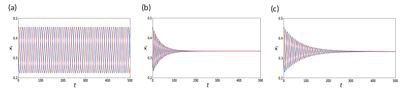
where and is odd. A circulant interaction matrix simplifies the modeling of species interactions by capturing regular, symmetrical patterns, making it easier to analyze coexistence and stability. It helps in predicting how cyclic or uniform interactions affect species dynamics and system stability. We further assume to prevent biologically implausible scenarios Grilli et al. (2017). Setting renders all elements of the interaction matrix equal to . This symmetry implies that each species exerts an identical influence on the others, effectively nullifying any cyclic dominance. Consequently, the species are indistinguishable in terms of competitive interaction, resulting in each having an equal probability of winning, with a chance in every interaction. For this matrix, the equilibrium point is . Since represents a winning probability matrix, sums like and are zero, leading to . By substituting these values into the equation , we confirm that . For example, with and , the matrix is . We illustrate the dynamics of our model for various values of and in Fig. (1), using initial densities of . In the following section, we will analytically demonstrate that these results hold qualitatively consistent for any initial densities within the range . It is important to note that for , selecting or any higher-order with is not possible.
II.2.1 Pairwise System
We consider pairwise interaction model as follows,
| (4) |
Now, we take the following Lyapunov function Chatterjee et al. (2022),
| (5) |
where is an odd integer. Now, we use Jensen’s inequality Jensen (1906); Ruel and Ayres (1999) as is a concave function. We find
| (6) | |||
Thus, clearly , for and
| (7) |
Now,
Since Grilli et al. (2017), we have
As a result, the system follows a closed orbit, cycling neutrally around the equilibrium point without ever reaching it unless it begins precisely at that point. As illustrated in Fig. 1(a), starting from the initial condition, the species densities oscillate around with a consistent amplitude that remains unchanged over time, indicating neutral cycling around the equilibrium point.
II.2.2 Non-pairwise System
We take the simplest possible non-pairwise system as follows,
| (8) |
We choose the same Lyapunov function (Eq. 5) for global stability analysis. We take a non-zero perturbation such that
| (9) |
Then, . Now,
Since and , we have
Thus, the system ultimately converges to a globally stable equilibrium point , determined by the interaction matrix . As shown in Fig. 1(b), over time, the oscillation amplitude decays, and the species densities gradually stabilize at the equilibrium point , reflecting a balanced coexistence where each species reaches equal abundance.
II.2.3 Mixed System
Below, we present a biologically motivated model that reflects real-world ecological dynamics by combining two critical components: pairwise interactions, which capture direct species interactions, and higher-order interactions, which account for more complex, multi-species interactions. This hybrid model allows us to explore how such mixed interactions influence ecosystem stability and species coexistence. This model is constructed as a convex combination of these two interaction types, expressed as follows:
| (10) |
Now again, we start with the same Lyapunov function (Eq. 5), and non-zero perturbation (Eq. 9) we arrive at,
Now, using the same simplification as mentioned in the above two analyses, we finally get for ,
Thus, in this model, the equilibrium point is globally stable, ensuring that regardless of any initial conditions except for a set of measure zero, the system will converge to this point over time. We adapt this definition of global stability from Refs. Kassabov et al. (2022); Nag Chowdhury et al. (2023a). Biologically, this reflects the stabilization of species densities, where all species reach a balanced state, coexisting at equal proportions. Numerically, as depicted in Figure 1(c), the system stabilizes at the equilibrium point , confirming the stability of the community dynamics.
II.3 Transient dynamics
In the pairwise interaction model, the system exhibits infinite transient time, with solutions continuously oscillating around the equilibrium point. However, introducing higher-order interactions significantly reduces this transient period, as observed in purely higher-order interaction models (See Fig. 1(b)). Our study will further investigate how incorporating both higher-order and mixed interactions can accelerate the reduction of transient time, leading to faster stabilization.
II.3.1 Effects of Shifting Balance from Pairwise to Higher-Order Interactions
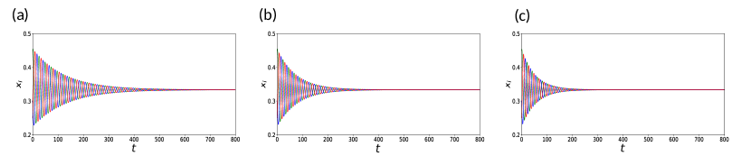
In Fig. 2, we examine how varying the proportion of pairwise versus higher-order interactions with affects the system dynamics. Despite different interaction ratios, the system consistently converges to the coexistence equilibrium, aligning with our previous analysis. Notably, as the contribution of higher-order interactions increases and the proportion of pairwise interactions decreases, the system reaches its equilibrium more rapidly. This observation raises a compelling question: why does the system achieve faster convergence with a higher proportion of higher-order interactions () and a correspondingly lower proportion of pairwise interactions? Biologically, this suggests that higher-order interactions may enhance the system’s ability to stabilize by facilitating more complex, cooperative dynamics among species, leading to quicker stabilization of community structure.
Before delving deeper into the analytical aspects of our results, we first aim to confirm that incorporating pairwise interactions into our system extends the transient time while increasing higher-order interactions shortens it. Figures 2 and 1 illustrate this trend with selected values for parameters and . To further validate this observation, we will explore a broader range of data.
II.3.2 Role of Initial Abundances in Systems with a Fixed Interaction Matrix
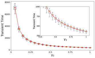
Two approaches can be employed to validate our findings. First, by fixing the interaction matrix and varying ecologically meaningful initial conditions, we can analyze how the transient time is influenced by and . We perform this analysis with as shown in Figure 3. It is well known that when , the system with only pairwise interactions does not converge to the coexistence equilibrium. Thus, we investigate the range with a small step-length of .
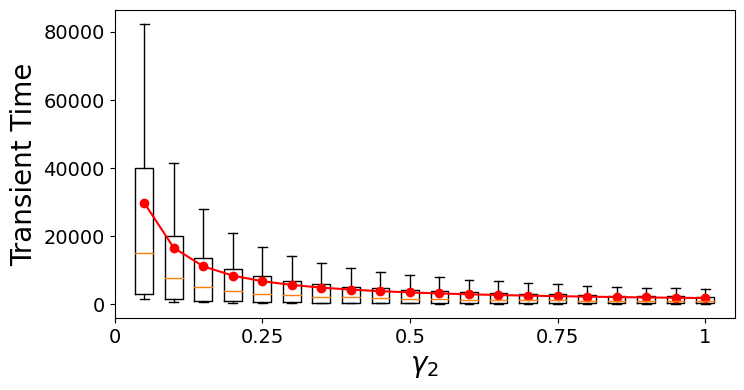
In Figure 3, transient times are summarized using a boxplot, with the median indicated by the yellow line and the mean by the red dot. Connecting lines between adjacent mean values provide a clearer view of the trend. As increases, indicating a higher proportion of higher-order interactions, mean transient times decrease. This suggests that ecosystems with more complex interactions can stabilize more rapidly, which is crucial for predicting how real-world ecosystems maintain biodiversity. An inset in the figure highlights the reduction in transient time, showing how quickly systems approach stability with higher-order interactions. To create this figure, we selected different random initial conditions, each constrained by . We measured the transient time for each condition—defined as the period until density oscillations fall below and then calculated the average of these transient times to obtain the mean value.
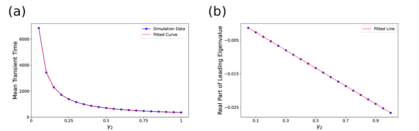
When , the system’s transient time is effectively infinite, leading to a rapid decline near zero and a more gradual decrease as increases. To quantify this relationship, we fitted the mean transient time for values ranging from to with a rectangular hyperbola fit in Fig. 4(a), illustrating how the product of mean transient time and remains constant, say , as increases. Our statistical analysis suggests that the value of this constant is with a Squared Error Loss of . The Squared Error Loss can be further reduced by increasing the number of initial data points, thereby providing a larger dataset for fitting. This fit provides a statistical measure of how swiftly the system’s transient time diminishes as the proportion of higher-order interactions increases. Note that the fitted inverse relationship between and the mean transient time indicates that as approaches , the mean transient time tends to infinity, which aligns with our observations. Moreover, the fit demonstrates that the transient duration decreases as increases, but this reduction occurs in a non-linear fashion. This finding highlights the significant impact of higher-order interactions on accelerating the system’s convergence to equilibrium.
II.3.3 Analytical Insights through Linear Theory
To further validate our results analytically, we employ linear algebraic theories. We use local stability analysis and examine the leading eigenvalues of the Jacobian matrix associated with the linearized system at the coexistence equilibrium. The leading eigenvalue is defined as the eigenvalue with the largest negative real part. The following table compares the leading eigenvalues for the system using the same parameter set as in Fig. 2.
| Parameter | Leading Pair of Eigenvalues |
|---|---|
The data clearly indicate that as increases and decreases, our non-hyperbolic dynamical system exhibits leading eigenvalues with increasingly larger negative real parts. This trend signifies that the system’s rate of convergence to the coexistence equilibrium point accelerates. Larger negative real parts in the leading eigenvalues correspond to a faster decay of perturbations, thereby reducing the time needed for the system to stabilize at the coexistence equilibrium. It’s important to note that the equilibrium point remains unchanged regardless of variations in nonzero values of and .
We have calculated the eigenvalues of the matrix for each value of and plotted the most negative real part in Fig. 4(b). The results show a clear linear trend with a slope of and a zero squared sum error, indicating a precise fit. This linear relationship highlights that as increases, the leading eigenvalues become more negative, which corresponds to faster convergence to the same coexistence equilibrium point. The increased negativity of the leading eigenvalue reflects enhanced stability and quicker decay of transient oscillations, underscoring how higher-order interactions expedite system stabilization.
We also compute the Jacobian matrix analytically for a three-species system at the coexistence equilibrium point, parameterized by constants and . Solving for the eigenvalues, we obtain:
Given that and , the nonzero eigenvalues of the matrix are always a pair of complex conjugates, each possessing both nonzero real and imaginary components. Thus, the real part of the dominant eigenvalue is:
which is always negative irrespective of any and . For , substituting the values yields , which is consistent with the negative slope obtained from the linear fit shown in Fig. 4.
For any linearized dynamical system, the general solution can be expressed as:
where are the time-independent eigenvectors and are the corresponding eigenvalues of the system Murphy (2011).
Let us define the following:
where and denote the real and imaginary parts of the eigenvalues, respectively.
In a small -neighborhood with near the equilibrium point, the solution to Eq. 1, i.e, the solution to linearised Eq. 1 for can be written as:
with , , and ’s are time-independent coefficients determined by the initial conditions of the system.
Since is negative in our non-hyberbolic system, the term represents an exponential decay. Although one of the eigenvalues is zero in our case, indicating the corresponding term neither decays nor grows, which prevents a conclusive determination of linear stability, we establish global stability through the construction of a suitable Lyapunov function. We can assert that the magnitude of governs the rate of convergence towards equilibrium, with the frequency of oscillation determined by the imaginary part . However, similar to how linear stability analysis is restricted to the vicinity of the equilibrium, the estimation of the convergence rate based on the real part of the leading eigenvalue is only valid within a local neighborhood of the equilibrium. Nonetheless, our analysis, grounded in the real part of the leading eigenvalues, offers a robust method for estimating the rate at which populations converge to coexistence abundances. Irrespective of the initial abundances, i.e., even if the populations begin at vastly different levels, the system will reliably move toward a balanced state of coexistence, where each species maintains a stable abundance, and our theoretical predictions regarding the rate of convergence towards the coexistence equilibrium align with observed dynamics in the system. This behavior is validated by the results shown in Table 1 and Fig. 4.
II.3.4 Effects of Varying Interaction Matrices with Fixed Initial Species Abundances
Up to this point, we have explored the influence of higher-order interactions by varying the initial conditions while keeping the interaction matrix fixed. Alternatively, one can take the opposite approach by keeping the initial condition constant and instead varying the interaction matrix . To explore how the structure of interaction impacts transient dynamics, we fix an initial condition randomly at , ensuring , and vary the interaction matrix by randomly sampling 20 values of from a uniform distribution over . For each , we generate different circulant matrices for and compute the mean transient time, which is plotted in Fig. 5. We observe that increasing consistently reduces transient time, confirming the influence of higher-order interactions on faster convergence. Notably, while varying the initial conditions slightly impacts the transient dynamics, the structure of interactions plays a far more dominant role in determining the transient times, as indicated by the significantly higher variance in transient times compared to different initial conditions. This suggests that the ecological architecture, particularly how species interact through both pairwise and higher-order interactions, exerts a stronger influence on system behavior than initial population distributions. Despite the changes in interaction matrices , the coexistence equilibrium remains constant, underscoring the resilience of the equilibrium point to structural variations in the interaction network. Our circulant matrices ensure that ecosystems with varying circulant interaction patterns will still converge to the same stable coexistence equilibrium. This highlights the role of symmetry and uniformity in maintaining stable ecological balances across diverse interaction networks. However, it should be noted that higher-order interactions accelerate convergence to equilibrium regardless of the interaction matrix structure Grilli et al. (2017).
II.3.5 Exploring Beyond First Higher Order Interactions
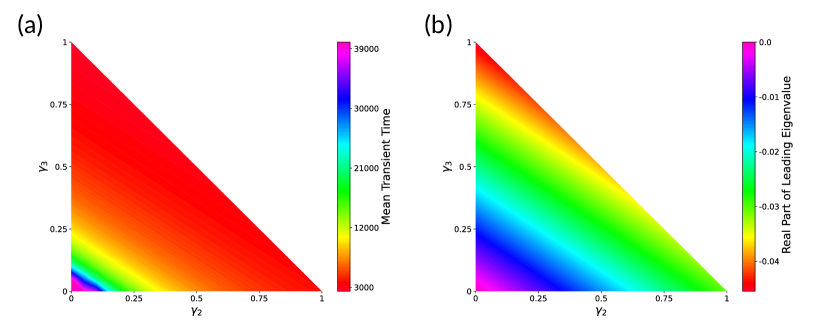
In previous analyses, we have examined systems incorporating only pairwise interactions and first higher-order interactions (HOIs). We now extend this investigation to include the effects of additional higher-order interactions. As more HOIs are introduced into the model, we observe that the transient time decreases and the system quickly converges to its equilibrium point. To analyze this phenomenon, we consider a model with pairwise interactions, first HOI, and second HOI, represented by the parameters , , and , respectively. This model adheres to the constraint:
By varying and , is automatically determined by the constraint, meaning when . When both and are zero, the system only includes pairwise interactions, resulting in an infinite transient time. Consequently, such scenarios are excluded from Fig. 6.
In the figure, the y-axis shows a more rapid decrease in transient time compared to the x-axis, indicating that second HOI significantly accelerate the system’s convergence relative to first HOI. Additionally, the gradient lines in the colormap are not parallel to the line , suggesting an asymmetry between the effects of and . This asymmetry highlights that second order interactions play a more influential role in reducing transient time than first order interactions, reflecting a more complex and nuanced impact of higher-order interactions on the dynamics of the system.
Now we analytically compute the Jacobian matrix for , incorporating both first and second higher-order interactions (HOIs) alongside pairwise interactions . Although the eigenvalues derived from this analysis are complicated and difficult to express explicitly, we gain better insight into their behavior by plotting them in a two-dimensional triangular space defined by the constraints , , and . This analysis aligns with our theoretical expectations; despite the non-hyperbolic nature of the model, the real part of the leading eigenvalue effectively reveals the system’s convergence rate toward the coexistence equilibrium. As shown in Fig. 6(b), there is a clear asymmetry, with exerting a stronger influence on the convergence dynamics than . It is important to note that while the transient time decays more rapidly in a non-linear fashion maintaining an inverse relationship with , the real part of the leading eigenvalue exhibits a linear trend for a fixed . Though both behaviors reflect the rate of convergence toward equilibrium, there is a subtle distinction between the patterns observed in the two subfigures. This behavior is consistent with the earlier observation in Fig. 4.
III Conclusion & Outlook
While previous studies have typically focused on either pairwise or higher-order interactions in isolation, our approach introduces a model that combines both types of interactions through a convex combination. We demonstrate significant differences in behavior between pairwise and higher-order interactions. By incorporating both interaction types, we analytically show that the system converges to a feasible coexistence equilibrium, utilizing appropriate Lyapunov functions for validation. While coexistence theory commonly assumes species interactions are pairwise Levine et al. (2017) and much of the literature examines how higher-order interactions (HOIs) affect the stability of species coexistence Letten and Stouffer (2019); Wilson (1992), the exploration of transient dynamics has received comparatively less empirical and theoretical attention. Our research addresses this gap by applying linear theory concepts to assess how HOIs influence transient dynamics in a simple replicator model of a complex multispecies community, considering the presence of pairwise interactions.
Our findings reveal that increasing the proportion of higher-order interactions accelerates the convergence to this equilibrium. This is due to higher-order interactions promoting a more efficient stabilization process, whereas pairwise interactions tend to prolong the transient phase, thereby slowing convergence. Although the linearized system with a combination of pairwise and higher-order interactions possesses a zero eigenvalue, the negative real parts of the leading eigenvalues of the Jacobian matrix associated with the linearized system at the coexistence equilibrium indicate that higher-order interactions contribute to faster convergence. This suggests that, biologically, systems with a greater fraction of higher-order interactions are more adept at reaching stable states, whereas pairwise interactions alone may impede this process by increasing transient dynamics.
This study employs a simplified replicator model to explore species interactions and their impact on biodiversity, acknowledging that while it does not capture all complexities of real-world systems, it remains valuable for examining various scenarios. Despite extensive research on replicator dynamics, our understanding of transient dynamics is limited due to a lack of established mathematical techniques. We aim to shed light on ecosystem behavior during transient periods, providing insights that may not only enhance our knowledge of ecosystem dynamics but also suggest pathways for more effective management and conservation practices. We focus on a simple replicator model, employing convex combinations to preserve the coexistence equilibrium while comparing transient times. Our model is biologically relevant, as it operates within the interval and reliably converges to the coexistence equilibrium. For simulations, we exclusively use circulant matrices that do not affect the coexistence equilibrium, allowing for meaningful comparisons of transient times. Driven by ecological considerations, we selected this model to explore how different interaction types influence transient dynamics. Our findings highlight the critical role of higher-order interactions in promoting quicker convergence to stable coexistence, which is essential for understanding adaptation and resistance in ecological systems.
Our framework offers fresh insights into natural systems where extended transient phases are prevalent. By integrating both pairwise and higher-order interactions, our model not only deepens the understanding of dynamic stabilization but also suggests new mechanisms for addressing prolonged transient behaviors. These concepts could pave the way for identifying and developing strategies to manage and mitigate such dynamics in ecological and evolutionary systems. We would like to clarify that our findings may not generalize to chaotic or more complex systems, as our analysis is grounded in linear and global stability methods, which are not suited for capturing chaotic dynamics. Likewise, the use of Lyapunov functions is limited to assessing equilibrium stability. We acknowledge that systems exhibiting chaotic behavior require alternative mathematical approaches, which are beyond the scope of this study. Exploring these complexities could offer valuable insights and represents a promising avenue for future research. Another potential avenue for future research is to explore how transient dynamics are affected by time-varying interactions Nag Chowdhury et al. (2019b); Ansarinasab et al. (2024a); Nag Chowdhury and Ghosh (2019); Mikaberidze et al. (2024); Dayani et al. (2023); Nag Chowdhury et al. (2020b, c); Ansarinasab et al. (2024b), a phenomenon commonly observed in natural systems. This remains a central and intriguing direction for future research, with the potential to uncover a broad range of fascinating outcomes.
acknowledgement
SC gratefully acknowledges Prof. Soumitra Banerjee for his deep insights and invaluable feedback during his time at IISER Kolkata, as well as Dr. Chittaranjan Hens for valuable discussions during SC’s lab visit to IIIT Hyderabad, funded by IIIT, and for his strong encouragement in pursuing this research. SNC thanks the National Science Foundation (Grant No. 1840221) for its support during his postdoctoral tenure at UC Davis, where the problem was first discussed with SC. Further in-depth discussions occurred during the 7th International Conference on Complex Dynamical Systems and Applications 2024 in Digha, India, while SNC was a visiting scientist at the Physics and Applied Mathematics Unit, Indian Statistical Institute, Kolkata. Gratitude is extended to Prof. Ulrike Feudel for the opportunity to discuss this work during this period. SNC also thanks Constructor University for its support during his postdoctoral tenure, during which the manuscript’s final stages were completed, and Prof. Syamal K. Dana for his valuable discussions at Dynamics Days Europe 2024 in Bremen, Germany, and his encouragement. Additionally, SNC expresses deep thanks to Prof. Alan Hastings for his insightful discussions at UC Davis and to his wife, Dr. Srilena Kundu, for her valuable suggestions, which significantly improved the manuscript.
References
- Lotka (1920) A. J. Lotka, Proceedings of the National Academy of Sciences 6, 410 (1920).
- Volterra (1926) V. Volterra, Animal Ecology , 409 (1926).
- May (1974) R. M. May, Science 186, 645 (1974).
- May and Leonard (1975) R. M. May and W. J. Leonard, SIAM journal on Applied Mathematics 29, 243 (1975).
- May (2019) R. M. May, Stability and complexity in model ecosystems (Princeton university press, 2019).
- Hastings (2001) A. Hastings, Ecology Letters 4, 215 (2001).
- Hastings et al. (2018) A. Hastings, K. C. Abbott, K. Cuddington, T. Francis, G. Gellner, Y.-C. Lai, A. Morozov, S. Petrovskii, K. Scranton, and M. L. Zeeman, Science 361, eaat6412 (2018).
- Lai and Tél (2011) Y.-C. Lai and T. Tél, Transient chaos: complex dynamics on finite time scales, Vol. 173 (Springer Science & Business Media, 2011).
- Biggs et al. (2009) R. Biggs, S. R. Carpenter, and W. A. Brock, Proceedings of the National Academy of Sciences 106, 826 (2009).
- Ludwig et al. (1978) D. Ludwig, D. D. Jones, C. S. Holling, et al., Journal of Animal Ecology 47, 315 (1978).
- Hutchinson (1961) G. E. Hutchinson, The American Naturalist 95, 137 (1961).
- Arnoldi et al. (2016) J.-F. Arnoldi, M. Loreau, and B. Haegeman, Journal of Theoretical Biology 389, 47 (2016).
- Cuddington (2011) K. Cuddington, Biological Theory 6, 203 (2011).
- Kuussaari et al. (2009) M. Kuussaari, R. Bommarco, R. K. Heikkinen, A. Helm, J. Krauss, R. Lindborg, E. Öckinger, M. Pärtel, J. Pino, F. Rodà, et al., Trends in Ecology & Evolution 24, 564 (2009).
- Ray et al. (2021) A. Ray, A. Pal, D. Ghosh, S. K. Dana, and C. Hens, Chaos: An Interdisciplinary Journal of Nonlinear Science 31 (2021).
- Tao et al. (2021) Y. Tao, J. L. Hite, K. D. Lafferty, D. J. Earn, and N. Bharti, Theoretical Ecology 14, 625 (2021).
- Norström et al. (2009) A. V. Norström, M. Nyström, J. Lokrantz, and C. Folke, Marine Ecology Progress Series 376, 295 (2009).
- Van Langevelde et al. (2003) F. Van Langevelde, C. A. Van De Vijver, L. Kumar, J. Van De Koppel, N. De Ridder, J. Van Andel, A. K. Skidmore, J. W. Hearne, L. Stroosnijder, W. J. Bond, et al., Ecology 84, 337 (2003).
- Scheffer et al. (1993) M. Scheffer, S. H. Hosper, M. L. Meijer, B. Moss, and E. Jeppesen, Trends in Ecology & Evolution 8, 275 (1993).
- Morozov et al. (2020) A. Morozov, K. Abbott, K. Cuddington, T. Francis, G. Gellner, A. Hastings, Y.-C. Lai, S. Petrovskii, K. Scranton, and M. L. Zeeman, Physics of Life Reviews 32, 1 (2020).
- Hobbs and Harris (2001) R. J. Hobbs and J. A. Harris, Restoration Ecology 9, 239 (2001).
- Neubert and Caswell (2000) M. G. Neubert and H. Caswell, Ecology 81, 1613 (2000).
- Hastings (2004) A. Hastings, Trends in Ecology & Evolution 19, 39 (2004).
- Shea and Chesson (2002) K. Shea and P. Chesson, Trends in Ecology & Evolution 17, 170 (2002).
- Hastings and Botsford (2006) A. Hastings and L. W. Botsford, Proceedings of the National Academy of Sciences 103, 6067 (2006).
- Scheffer et al. (2005) M. Scheffer, S. Carpenter, and B. de Young, Trends in Ecology & Evolution 20, 579 (2005).
- Murdoch et al. (2003) W. Murdoch, C. Briggs, and R. Nisbet, “Consumer-resource dynamics. princeton university press,” (2003).
- Schreiber and Rudolf (2008) S. Schreiber and V. H. Rudolf, Ecology Letters 11, 576 (2008).
- Holt (2008) R. D. Holt, Ecology 89, 671 (2008).
- Dudkowski et al. (2022) D. Dudkowski, P. Jaros, and T. Kapitaniak, Chaos: An Interdisciplinary Journal of Nonlinear Science 32 (2022).
- Nag Chowdhury and Ghosh (2020) S. Nag Chowdhury and D. Ghosh, The European Physical Journal Special Topics 229, 1299 (2020).
- Koch et al. (2024) D. Koch, A. Nandan, G. Ramesan, I. Tyukin, A. Gorban, and A. Koseska, Physical Review Letters 133, 047202 (2024).
- Nag Chowdhury et al. (2020a) S. Nag Chowdhury, D. Ghosh, and C. Hens, Physical Review E 101, 022310 (2020a).
- Bovier and Den Hollander (2016) A. Bovier and F. Den Hollander, Metastability: a potential-theoretic approach, Vol. 351 (Springer, 2016).
- Kelso (2012) J. S. Kelso, Philosophical Transactions of the Royal Society B: Biological Sciences 367, 906 (2012).
- Parastesh et al. (2022) F. Parastesh, M. Mehrabbeik, K. Rajagopal, S. Jafari, and M. Perc, Chaos: An Interdisciplinary Journal of Nonlinear Science 32 (2022).
- Mehrabbeik et al. (2023a) M. Mehrabbeik, S. Jafari, and M. Perc, Frontiers in Computational Neuroscience 17, 1248976 (2023a).
- Alvarez-Rodriguez et al. (2021) U. Alvarez-Rodriguez, F. Battiston, G. F. de Arruda, Y. Moreno, M. Perc, and V. Latora, Nature Human Behaviour 5, 586 (2021).
- Pal et al. (2024) P. K. Pal, M. S. Anwar, M. Perc, and D. Ghosh, Physical Review Research 6, 033003 (2024).
- Ma et al. (2024) Y.-J. Ma, Z.-Q. Jiang, F.-S. Fang, M. Perc, and S. Boccaletti, Proceedings of the Royal Society A 480, 20240066 (2024).
- Anwar et al. (2024) M. S. Anwar, G. K. Sar, M. Perc, and D. Ghosh, Communications Physics 7, 59 (2024).
- Mirzaei et al. (2022) S. Mirzaei, M. Mehrabbeik, K. Rajagopal, S. Jafari, and G. Chen, Chaos: An Interdisciplinary Journal of Nonlinear Science 32 (2022).
- Mehrabbeik et al. (2023b) M. Mehrabbeik, A. Ahmadi, F. Bakouie, A. H. Jafari, S. Jafari, and D. Ghosh, Mathematics 11, 2811 (2023b).
- Chatterjee et al. (2023a) S. Chatterjee, A. N. Zehmakan, and S. Rastogi, Chaos, Solitons & Fractals 177, 114297 (2023a).
- Vasilyeva et al. (2021) E. Vasilyeva, A. Kozlov, K. Alfaro-Bittner, D. Musatov, A. Raigorodskii, M. Perc, and S. Boccaletti, Scientific Reports 11, 5666 (2021).
- Alvarez-Rodriguez et al. (2022) U. Alvarez-Rodriguez, F. Battiston, G. Ferraz de Arruda, Y. Moreno, M. Perc, and V. Latora, in Higher-order systems (Springer, 2022) pp. 377–388.
- Majhi et al. (2022) S. Majhi, M. Perc, and D. Ghosh, Journal of the Royal Society Interface 19, 20220043 (2022).
- Kumar et al. (2021) A. Kumar, S. Chowdhary, V. Capraro, and M. Perc, Physical Review E 104, 054308 (2021).
- Ray et al. (2022) A. Ray, T. Bröhl, A. Mishra, S. Ghosh, D. Ghosh, T. Kapitaniak, S. K. Dana, and C. Hens, Chaos: An Interdisciplinary Journal of Nonlinear Science 32 (2022).
- Nag Chowdhury et al. (2024) S. Nag Chowdhury, M. S. Anwar, and D. Ghosh, Physical Review E 109, 044314 (2024).
- Ray et al. (2020) A. Ray, S. Kundu, and D. Ghosh, Europhysics Letters 128, 40002 (2020).
- Nag Chowdhury et al. (2023a) S. Nag Chowdhury, S. Rakshit, C. Hens, and D. Ghosh, Physical Review E 107, 034313 (2023a).
- Chatterjee and Zehmakan (2023) S. Chatterjee and A. N. Zehmakan, Chaos, Solitons & Fractals 175, 113952 (2023).
- Nag Chowdhury et al. (2019a) S. Nag Chowdhury, S. Majhi, D. Ghosh, and A. Prasad, Physics Letters A 383, 125997 (2019a).
- Battiston et al. (2020) F. Battiston, G. Cencetti, I. Iacopini, V. Latora, M. Lucas, A. Patania, J.-G. Young, and G. Petri, Physics Reports 874, 1 (2020).
- Gibbs et al. (2022) T. Gibbs, S. A. Levin, and J. M. Levine, Proceedings of the National Academy of Sciences 119, e2205063119 (2022).
- Zhang et al. (2023) Y. Zhang, M. Lucas, and F. Battiston, Nature Communications 14, 1605 (2023).
- Battiston et al. (2021) F. Battiston, E. Amico, A. Barrat, G. Bianconi, G. Ferraz de Arruda, B. Franceschiello, I. Iacopini, S. Kéfi, V. Latora, Y. Moreno, et al., Nature Physics 17, 1093 (2021).
- Terry et al. (2020) J. C. D. Terry, M. B. Bonsall, and R. J. Morris, Oikos 129, 147 (2020).
- Li et al. (2021) Y. Li, M. M. Mayfield, B. Wang, J. Xiao, K. Kral, D. Janik, J. Holik, and C. Chu, National Science Review 8, nwaa244 (2021).
- Raj et al. (2024) U. Raj, A. Banerjee, S. Ray, and S. Bhattacharya, PloS One 19, e0306409 (2024).
- Kleinhesselink et al. (2022) A. R. Kleinhesselink, N. J. Kraft, S. W. Pacala, and J. M. Levine, Ecology Letters 25, 1604 (2022).
- Barbosa et al. (2023) M. Barbosa, G. W. Fernandes, and R. J. Morris, Current Biology 33, 381 (2023).
- Chase and Leibold (2009) J. M. Chase and M. A. Leibold, Ecological Niches (University of Chicago Press, 2009).
- Soberón and Nakamura (2009) J. Soberón and M. Nakamura, Proceedings of the National Academy of Sciences 106, 19644 (2009).
- Brokaw and Busing (2000) N. Brokaw and R. T. Busing, Trends in Ecology & Evolution 15, 183 (2000).
- Huisman and Weissing (1999) J. Huisman and F. J. Weissing, Nature 402, 407 (1999).
- Clark and McLachlan (2003) J. S. Clark and J. S. McLachlan, Nature 423, 635 (2003).
- Nag Chowdhury et al. (2023b) S. Nag Chowdhury, J. Banerjee, M. Perc, and D. Ghosh, Journal of Theoretical Biology 564, 111446 (2023b).
- Park et al. (2017) J. Park, Y. Do, B. Jang, and Y.-C. Lai, Scientific Reports 7, 1 (2017).
- Nagatani et al. (2019) T. Nagatani, G. Ichinose, and K.-i. Tainaka, Journal of Theoretical Biology 462, 425 (2019).
- Nag Chowdhury et al. (2021a) S. Nag Chowdhury, S. Kundu, M. Perc, and D. Ghosh, Proceedings of the Royal Society A 477, 20210397 (2021a).
- Roy et al. (2022) S. Roy, S. Nag Chowdhury, P. C. Mali, M. Perc, and D. Ghosh, PLoS One 17, e0272719 (2022).
- Roy et al. (2023) S. Roy, S. Nag Chowdhury, S. Kundu, G. K. Sar, J. Banerjee, B. Rakshit, P. C. Mali, M. Perc, and D. Ghosh, Scientific Reports 13, 14331 (2023).
- Nagatani (2019) T. Nagatani, Physica A: Statistical Mechanics and its Applications 535, 122531 (2019).
- Ahmadi et al. (2023) A. Ahmadi, S. Roy, M. Mehrabbeik, D. Ghosh, S. Jafari, and M. Perc, Plos One 18, e0283757 (2023).
- Nag Chowdhury et al. (2021b) S. Nag Chowdhury, S. Kundu, J. Banerjee, M. Perc, and D. Ghosh, Journal of Theoretical Biology 518, 110606 (2021b).
- Yang and Park (2023) R. K. Yang and J. Park, Chaos, Solitons & Fractals 175, 113949 (2023).
- Kirkup and Riley (2004) B. C. Kirkup and M. A. Riley, Nature 428, 412 (2004).
- Laird and Schamp (2006) R. A. Laird and B. S. Schamp, The American Naturalist 168, 182 (2006).
- Hibbing et al. (2010) M. E. Hibbing, C. Fuqua, M. R. Parsek, and S. B. Peterson, Nature Reviews Microbiology 8, 15 (2010).
- Szolnoki et al. (2014) A. Szolnoki, M. Mobilia, L.-L. Jiang, B. Szczesny, A. M. Rucklidge, and M. Perc, Journal of the Royal Society Interface 11, 20140735 (2014).
- Bhattacharyya et al. (2020) S. Bhattacharyya, P. Sinha, R. De, and C. Hens, Physical Review E 102, 012220 (2020).
- Islam et al. (2022) S. Islam, A. Mondal, M. Mobilia, S. Bhattacharyya, and C. Hens, Physical Review E 105, 014215 (2022).
- Chatterjee et al. (2023b) S. Chatterjee, R. De, C. Hens, S. K. Dana, T. Kapitaniak, and S. Bhattacharyya, Scientific Reports 13, 20740 (2023b).
- Soliveres et al. (2015) S. Soliveres, F. T. Maestre, W. Ulrich, P. Manning, S. Boch, M. A. Bowker, D. Prati, M. Delgado-Baquerizo, J. L. Quero, I. Schöning, et al., Ecology Letters 18, 790 (2015).
- Cameron et al. (2009) D. D. Cameron, A. White, and J. Antonovics, Journal of Ecology 97, 1311 (2009).
- Malizia et al. (2024) F. Malizia, A. Corso, L. V. Gambuzza, G. Russo, V. Latora, and M. Frasca, Nature Communications 15, 5184 (2024).
- Kundu and Ghosh (2022) S. Kundu and D. Ghosh, Physical Review E 105, L042202 (2022).
- Van Giel et al. (2024) T. Van Giel, A. J. Daly, J. M. Baetens, and B. De Baets, arXiv preprint arXiv:2408.14209 (2024).
- Gibbs et al. (2024) T. L. Gibbs, G. Gellner, S. A. Levin, K. S. McCann, A. Hastings, and J. M. Levine, Ecology Letters 27, e14458 (2024).
- Singh and Baruah (2021) P. Singh and G. Baruah, Theoretical Ecology 14, 71 (2021).
- Grilli et al. (2017) J. Grilli, G. Barabás, M. J. Michalska-Smith, and S. Allesina, Nature 548, 210 (2017).
- Chatterjee et al. (2022) S. Chatterjee, S. Nag Chowdhury, D. Ghosh, and C. Hens, Chaos: An Interdisciplinary Journal of Nonlinear Science 32 (2022).
- Schuster and Sigmund (1983) P. Schuster and K. Sigmund, Journal of Theoretical Biology 100, 533 (1983).
- Roca et al. (2009) C. P. Roca, J. A. Cuesta, and A. Sánchez, Physics of Life Reviews 6, 208 (2009).
- Börgers and Sarin (1997) T. Börgers and R. Sarin, Journal of Economic Theory 77, 1 (1997).
- Nag Chowdhury et al. (2021c) S. Nag Chowdhury, A. Ray, A. Mishra, and D. Ghosh, Journal of Physics: Complexity 2, 035021 (2021c).
- Hofbauer and Sigmund (1998) J. Hofbauer and K. Sigmund, Evolutionary games and population dynamics (Cambridge university press, 1998).
- Jensen (1906) J. L. W. V. Jensen, Acta Mathematica 30, 175 (1906).
- Ruel and Ayres (1999) J. J. Ruel and M. P. Ayres, Trends in Ecology & Evolution 14, 361 (1999).
- Kassabov et al. (2022) M. Kassabov, S. H. Strogatz, and A. Townsend, Chaos: An Interdisciplinary Journal of Nonlinear Science 32 (2022).
- Murphy (2011) G. M. Murphy, Ordinary differential equations and their solutions (Courier Corporation, 2011).
- Levine et al. (2017) J. M. Levine, J. Bascompte, P. B. Adler, and S. Allesina, Nature 546, 56 (2017).
- Letten and Stouffer (2019) A. D. Letten and D. B. Stouffer, Ecology Letters 22, 423 (2019).
- Wilson (1992) D. S. Wilson, Ecology 73, 1984 (1992).
- Nag Chowdhury et al. (2019b) S. Nag Chowdhury, S. Majhi, M. Ozer, D. Ghosh, and M. Perc, New Journal of Physics 21, 073048 (2019b).
- Ansarinasab et al. (2024a) S. Ansarinasab, F. Nazarimehr, F. Ghassemi, D. Ghosh, and S. Jafari, Applied Mathematics and Computation 468, 128508 (2024a).
- Nag Chowdhury and Ghosh (2019) S. Nag Chowdhury and D. Ghosh, Europhysics Letters 125, 10011 (2019).
- Mikaberidze et al. (2024) G. Mikaberidze, S. Nag Chowdhury, A. Hastings, and R. M. D’Souza, Chaos, Solitons & Fractals 178, 114298 (2024).
- Dayani et al. (2023) Z. Dayani, F. Parastesh, F. Nazarimehr, K. Rajagopal, S. Jafari, E. Schöll, and J. Kurths, Chaos: An Interdisciplinary Journal of Nonlinear Science 33 (2023).
- Nag Chowdhury et al. (2020b) S. Nag Chowdhury, S. Kundu, M. Duh, M. Perc, and D. Ghosh, Entropy 22, 485 (2020b).
- Nag Chowdhury et al. (2020c) S. Nag Chowdhury, S. Majhi, and D. Ghosh, IEEE Transactions on Network Science and Engineering 7, 3159 (2020c).
- Ansarinasab et al. (2024b) S. Ansarinasab, F. Nazarimehr, G. K. Sar, F. Ghassemi, D. Ghosh, S. Jafari, and M. Perc, Nonlinear Dynamics , 1 (2024b).