Evaluating probabilistic and data-driven inference models for fiber-coupled NV-diamond temperature sensors

Abstract

We evaluate the impact of inference model on uncertainties when using continuous wave Optically Detected Magnetic Resonance (ODMR) measurements to infer temperature. Our approach leverages a probabilistic feedforward inference model designed to maximize the likelihood of observed ODMR spectra through automatic differentiation. This model effectively utilizes the temperature dependence of spin Hamiltonian parameters to infer temperature from spectral features in the ODMR data. We achieve prediction uncertainty of $\pm$ 1 K across a temperature range of 243 K to 323 K. To benchmark our probabilistic model, we compare it with a non-parametric peak-finding technique and data-driven methodologies such as Principal Component Regression (PCR) and a 1D Convolutional Neural Network (CNN). We find that when validated against out-of-sample dataset that encompasses the same temperature range as the training dataset, data driven methods can show uncertainties that are as much as 0.67 K lower without incorporating expert-level understanding of the spectroscopic-temperature relationship. However, our results show that the probabilistic model outperforms both PCR and CNN when tasked with extrapolating beyond the temperature range used in training set, indicating robustness and generalizability. In contrast, data-driven methods like PCR and CNN demonstrate up to ten times worse uncertainties when tasked with extrapolating outside their training data range.

1 Introduction

Temperature is a critical parameter in various aspects of modern life, including manufacturing processes [1], medical procedures, and environmental control of residential and commercial spaces. To meet such disparate measurement needs, a variety of temperature sensors have been developed. Although these devices vary greatly in their cost, size, weight and complexity, they almost all rely on well-established measurements of transport properties to infer temperature. Legacy technologies like platinum resistance thermometers and negative temperature coefficient thermistors have been relied upon for over a century to provide accurate and reproducible measurements over a broad range of temperature[2, 3, 4]. However, these sensors are prone to drift and require frequent re-calibrations to ensure high accuracy in critical use-cases resulting in increase cost of sensor ownership.

In recent years, there has been a growing interest in developing alternative sensor technologies that can overcome the limitations of traditional technologies. The past decade has seen a burst of activity in nanophotonics[5], quantum optomechanics[6] and noise thermometry[7]. These technologies leverage telecomm industry’s vast economies of scale along with precision measurement expertise developed for frequency metrology to enable fit-for-purpose, cost-effective measurement solutions. Development of an ultra-stable temperature sensor that shows minimal drift over decadal time spans or a field-deployable thermodynamic temperature sensor, likely based on quantum technologies could disrupt the calibration-centered metrology ecosystem of today [4, 5]. Chip-based photonic and quantum thermometry technologies, such as photonic ring resonators, are well-suited for macroscale sensors that address the industrial needs of today. However, the emerging field of nanoscale heat transport in complex systems, such as quantum information systems [4], biological matrices, and advanced computer chips, demands the development of novel nanoscale temperature sensors.

In this context, nitrogen-vacancy (NV) in diamond has emerged as a potential candidate technology to enable temperature measurements at micro and nanoscale distances. These sensors leverage the sensitivity of NV spin systems to environmental magnetic and electrical fields [8, 9] along with sensitivity to local temperature and pressure to enable high sensitivity. While NV has garnered considerable attention for quantum magnetometry applications, its sensitivity to temperature has led to suggestion that it may be suitable for temperature measurement applications in embedded systems such as temperature control in microfluidics [10], generating heatmaps of the surrounding environment of thin metallic wires [11], and measuring temperature of living cells [12]. Temperature sensitivities on the order of $10\ \mathrm{mK}/\sqrt{\mathrm{Hz}}$ have been reported [12, 13] using pulsed optically detected magnetic resonance (pulsed-ODMR) highlighting the potential of NV thermometry. Recent technological advancements, such as integration with optical fiber probes [13, 14] have expanded the potential for practical applications of NV sensors. Using continuous-wave ODMR measurement, researcher’s have reported sensitivities of $2\ \mathrm{K}/\sqrt{\mathrm{Hz}}$[15].

In this work, we assess how different inference models affect uncertainties by comparing data-driven and model-based approaches for temperature estimation. The model-based approach relies on a probabilistic feedforward inference model based on NV’s Hamiltonian that is used to infer temperature from NV’s optically detected magnetic resonance (ODMR) spectra acquired using a fiber-coupled NV temperature sensor. This probabilistic model is compared to non-parametric peak-finding routines and unsupervised learning techniques such as Principal Component Regression (PCR) [16] and Convolutional Neural Network (CNN) [17]. The later two methodologies are entirely data-driven and do not rely on any expert/physics-based insights on the relationship between spectroscopic features and temperature. Our results demonstrate physics-based probabilistic model is competitive with data-driven models. Data-driven models, when tested with out-of-sample data, outperforms the probabilistic model. However, when tasked with extrapolating beyond the training range, data-driven models vastly underperform against the probabilistic model.

2 METHODS

2.1 Experimental setup

The experimental setup described below is used to perform continuous wave ODMR measurements on a fiber-coupled NV sensor. The sensor is fabricated by affixing a $\approx 150\ \mu\text{m}$ diameter diamond particle with $\approx$3.5$\,\mu\text{mol/mol}$ of NV color centers (Adamas Nanotechnologies) using $\approx 1\,\text{µL}$ of UV curable optically clear epoxy (EPOTEK 301 G) onto port 3 of a wide band circulator (Thorlabs). A $50\ \mu\text{m}$ diameter radio frequency (RF) wire is epoxied ontop of the micro-diamond. Port 1 of the wide band circulator is connected to a fiber-coupled 514 nm laser (LABS electronics p/n: DLnsec) whilst port 3 delivers the light to detector assembly, where long and short pass filters are used to selectively transmit light between 633 nm and 800 nm only. The filtered light is passed onto a 10X objective that focuses the light into a multimode $105\ \mu\text{m}$ diameter optical fiber. The light is then carried to a photon counting module (Laser Components, p/n: COUNT-500). The photon detector’s output is sent to a data acquisition card (National Instruments, NI-6363) via a coaxial cable.

The measurement system relies on a 514 nm laser to spin polarize the NV system and readout the spin. RF power across frequency range of 2.82 GHz to 2.92 GHz is sequentially generated by a signal generator (Stanford Instruments p/n: 384) in preprogrammed steps of 300 kHz to 1 MHz to address the spin. The RF power is amplified using a high-power amplifier (Mini-Circuits p/n: ZHL-15W-45S+) and output chopped into on/off pulses using a RF switch (Mini-Circuits p/n: ZASWA-2-50DRA+) before being delivered to the sample. The timing of RF switch and data acquisition card is synchronized by an external transitor-transitor logic (TTL) card (Spincore p/n: PulseBlaster-PRO-500). For temperature measurements, the sensor is immersed in a metrology-grade drywell (Fluke p/n: 9170) whose temperature is linearly ramped up and down between 243 K and 323 K at 5 K steps. During temperature steps, the temperature is raised at a steady rate of 1 K/min. Once the drywell reaches the target temperature, an additional 15 mins of equilibriation period was enforced before ODMR measurements were collected. For each temperature measurement 20 frequency scans were acquired and averaged.

As a standard pre-processing step, spectral normalization is applied. The normalization procedure serves to achieve uniformity across spectra by zero-centering the data and scaling the maximum intensity to a reference value, ensuring consistency among spectra.

Finally, each method of estimating temperature is evaluated using in-sample and out-of-sample data sets. Dividing the data into in-sample and out-of-sample sets enables each methodology to show its ability to generalize to new, unseen data, which is essential for accurately inferring temperatures across diverse experimental conditions and sample variations. Furthermore, each method’s performance can be evaluated by comparing the predicted temperatures with the measured temperatures for the out-of-sample data, providing insights into the method’s accuracy, robustness, and potential for further improvement or fine-tuning. The out-of-sample and in-sample prediction uncertainties for each model are presented in Table 1 and Table 2 , respectively. In Table 3 , each model’s output is augemented with an additional linear regression to correct for bias introduced by the linear assumption.

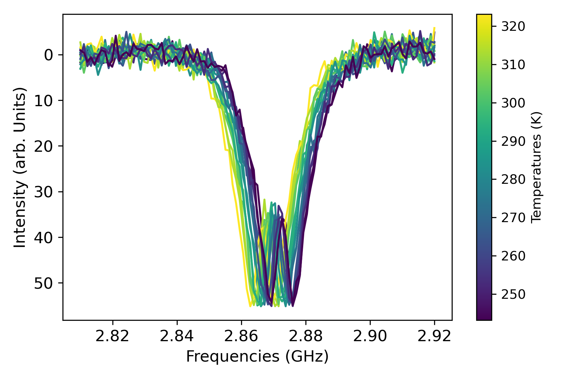
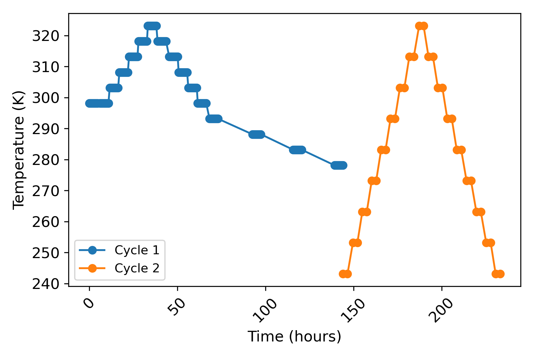
Figure 1: Left: ODMR spectra across a temperature range of 243.14 K to 323.15 K. Note that the spectra do not show any significant changes in contrast and width. Right: Temperature history of the sensor over cycle 1 and 2.

2.2 Estimating temperature: a model based approach

2.2.1 Overview of the model

The behavior of the NV center in diamond is governed by its spin Hamiltonian Eq. (1), which describes the energy levels and dynamics of the electron spin[18].

$$\hat{H}=\hbar D\left[\hat{S}_{Z}^{2}-\frac{2}{3}\right]+\hbar E\left(\hat{S}_{X}^{2}-\hat{S}_{Y}^{2}\right)$$ (1)

where $\hbar$ is the reduced Planck constant, $D$ is the axial zero-field splitting parameter, $E$ is the non-axial zero-field splitting parameter, and $\hat{S}_{X}$, $\hat{S}_{Y}$, and $\hat{S}_{Z}$ are the spin operators. The axial parameter $D$ is particularly sensitive to changes in temperature and primarily governs the center frequency of the ODMR spectrum. In contrast, the non-axial parameter $E$ has a weaker temperature dependence and mainly influences the splitting frequency between resonance peaks in the ODMR spectrum. The temperature dependence of $D$ and $E$ is typically described by linear equations, as shown in equations Eq. (2) and Eq. (3), where $T$ is the temperature and $a$, $b$, $c$, and $d$ are constants specific to the NV center system. Notably, constants $c$ and $d$ are treated as fixed using literature values [19] $c=-4.65\times 10^{-7}\,\text{GHz}/\text{K}$ and $d=0.0052\,\text{GHz}/\text{K}$.

$$D=aT+b$$ (2)

$$E=cT+d$$ (3)

The actual observed ODMR spectrum is modeled as a combination of two Lorentzian functions (bi-Lorentzian), as shown in Figure 2, centered at transition frequencies corresponding to the spin Hamiltonian’s eigenvalues, with additional Gaussian noise. By incorporating temperature into the $D$ and $E$ parameters, which in turn affect the Hamiltonian’s eigenvalues, it becomes possible to determine the peak centers in the ODMR spectrum. To fully specify the model, the widths and amplitudes of the Lorentzian functions, as well as the parameters $a$ and $b$ relating $D$ and $E$ to temperature, needs to be determined. Once these parameters are known, the model can calculate the likelihood of observing a given ODMR spectrum for different temperature values.

The key idea is to use a probabilistic feedforward inference approach [20] to find the temperature value that maximizes the likelihood of the observed ODMR spectrum, effectively utilizing the temperature dependence of the spin Hamiltonian parameters to infer the temperature from the observed spectral features in the ODMR spectrum. The use of Maximum Likelihood Estimation (MLE) provides an additional level of flexibility, namely, the model can be readily adapted to single spin-single photon measurements by changing the noise model from Gaussian to Poisson. In the case of ensemble measurements, a Gaussian noise model is appropriate and the MLE model behaves similar to a least squares model but also allows maximum likelihood parameter estimation.

2.2.2 Fitting model parameters

To fully specify the model, we conduct a fitting procedure using a bi-Lorentzian function applied to the observed ODMR spectrum. As illustrated in Figure 2, bi-Lorentzians fit the ODMR profile of both a packaged i.e. fiberized NV sensor and an "unpackaged" single crystal chip suggesting the use of Lorentzians under low laser and microwave power is broadly applicable to bulk NV sensors. This fitting process allow us to determine the nominal values of amplitudes and widths of the Lorentzian components over the temperature examined here. Over the temperature examined here, amplitude and width show little temperature dependent variation, as such we treat these variables as being temperature independent in our model.

Once the Lorentzian parameters have been determined, we can proceed to estimate the temperature-dependent coefficients, $a$ and $b$, using Maximum Likelihood Estimation (MLE) optimization. The MLE approach involves constructing a likelihood function that quantifies the probability of observing the given spectroscopic data for the coefficients $a$ and $b$.

The overall likelihood for all spectra can be expressed as:

$$L(\text{all spectrum}\mid a,b)=\prod_{i=1}^{M}L_{i}(\text{spectrum}_{i}\mid a,b)$$ (4)

where $M$ is the total number of spectra, and $L_{i}(\text{spectrum}_{i}\mid a,b)$ is the likelihood of observing the $i$-th spectrum given $a$ and $b$. This product represents the assumption that the spectra are independent observations.

During model fitting, we sum the log-likelihoods of all spectra (equation 4) and maximize them with respect to $a$ and $b$ using Powell’s conjugate direction method [21]. This derivative-free optimization method possesses the capability to handle multiple variables and is applicable to non-linear functions. Its simplicity of implementation, which circumvents extensive parameter tuning, renders Powell’s conjugate direction method a fitting choice for maximizing the log-likelihood function. Once $a$ and $b$ are determined, we fix these values and maximize the log-likelihood with respect to temperature for any single spectrum, as discussed in the subsequent section.

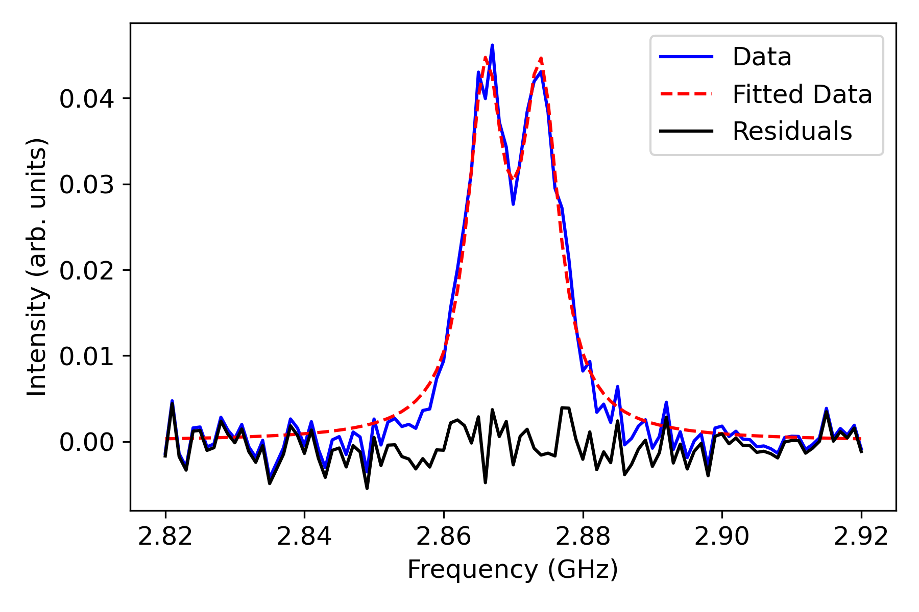
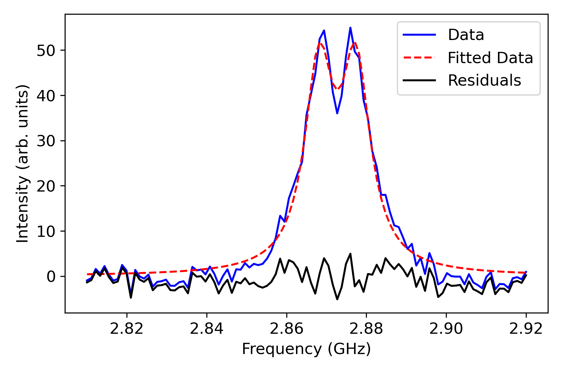
Figure 2: ODMR spectra of NV chip (Element six) and fiber coupled microparticle are fitted to bi-lorentzian function. The suitability of fit shows that 2 -Lorentzian function can be used across wide range of NV sensors regardless of their origin. The flat residuals indicate Lorentzian function is sufficient to capture spectral line shape.

2.3 Running the model

Our objective is to determine the most accurate estimates for temperature using MLE based on spectroscopy data. This entails creating a likelihood function, which relies on Gaussian distributions, and identifying the parameter values that maximize it. The likelihood function assesses how well the bi-Lorentzian function $\mathcal{S}_{k,i}(T)$ evaluated at the $k$-th frequency point for the $i$-th spectrum, with temperature $T$ fits the observed data $m_{k,i}$ at a specific frequency $k$. It originates from photon observations, considering the probability of encountering a particular number of photons while factoring in the expected rate of photon occurrences over time.

Each measurement $m_{k,i}$ is assumed to follow a Gaussian distribution centered around the expected value $\mu_{k,i}$ with standard deviation $\sigma_{k,i}$. The likelihood function for observing $m_{k,i}$ given $\mu_{k,i}$ is:

$$L(m_{k,i}\mid\mu_{k,i})=\frac{1}{\sqrt{2\pi}\sigma_{k,i}}\exp\left(-\frac{(m_{k,i}-\mu_{k,i})^{2}}{2\sigma_{k,i}^{2}}\right)$$ (5)

The expected value $\mu_{k,i}$ is modeled by the bi-Lorentzian spectrum function, scaled by the known parameters $\Delta t$ and $r$

$$\mu_{k,i}=\Delta t\,r\,\mathcal{S}_{k,i}(T)$$ (6)

The likelihood of a single spectrum consisting of $N_{i}$ measurements is given by:

$$L(m_{1,i},m_{2,i},\ldots,m_{N_{i}}\mid T)=\prod_{k=1}^{N_{i}}\frac{1}{\sqrt{2\pi}\sigma_{k,i}}\exp\left(-\frac{(m_{k,i}-\Delta t\,r\,\mathcal{S}_{k,i}(a,b,T))^{2}}{2\sigma_{k,i}^{2}}\right)$$ (7)

To facilitate optimization, we consider the log-likelihood function. Taking the natural logarithm of the likelihood function:

$$\log\mathcal{L}_{i}(\text{spectrum}_{i}\mid T)=\sum_{k=1}^{N_{i}}\left[-\log(\sqrt{2\pi}\sigma_{k,i})-\frac{(m_{k,i}-\Delta t\,r\,\mathcal{S}_{k,i}(a,b,T))^{2}}{2\sigma_{k,i}^{2}}\right]$$ (8)

Now, the focus is on optimizing the log-likelihood function (equation  8), which relies on the Hamiltonian via its eigenvalues. A significant hurdle in MLE arises when computing derivatives with respect to temperature. While theoretical formulas for these derivatives exist, as demonstrated in [22], modern programming favors more efficient methods for computation. Here we employ automatic differentiation as the preferred approach [23].

To leverage automatic differentiation effectively, we rely on TensorFlow [24], a widely adopted library for machine learning and scientific computation. In order to quickly maximize the log-likelihood function, and find the MLE temperature, it is helpful to find the derivative of the log-likelihood with respect to temperature, however this is challenging since computing the log-likelihood involves solving an eigenvalue problem for the Hamiltonian. TensorFlow enables us to easily compute the this complicated derivative, by using automatic differentiation to find the derivative of the eigensolver. Subsequently, we utilize the optimization functionalities provided by the SciPy [25] library. Specifically, we employ the Newton-CG (Conjugate Gradient) optimization algorithm, which is a specialized refinement of Newton’s method tailored for problems with small feature spaces. Newton’s method typically involves computing and inverting the Hessian matrix, which can be computationally intensive for large feature sets. However, Newton-CG is designed to address this issue by combining Newton’s method with the Conjugate Gradient approach, thereby avoiding the direct computation of the Hessian inverse. This hybrid approach facilitates rapid convergence while managing computational efficiency, making it well-suited for scenarios with a relatively small number of features. The algorithm iteratively refines our parameter estimates by minimizing the negative log-likelihood function until convergence is achieved.

The depiction in Figure  3 sheds light on the excellent correlation between temperature reported by the drywell and predicted temperatures during cycle 2 of a fiber-coupled NV sensor using parameters derived from cycle 1. The close match between the drywell’s measured temperature and the model’s predicted temperatures demonstrates the effectiveness of our method in capturing temperature variations within spectroscopy data. This is evidenced by a root mean squared error (RMSE) of $<2$ K, as shown in Table 1 and 2.

We note that fitting cycle 2 using parameters specific to cycle 2 obtained nearly identical results with an RMSE between measured and predicted temperatures of $1.74$ K, indicating little or no hysteresis between the two thermal cycles. The residuals associated with cycle 2 shown in Figure  3 (right panel) are zero-mean centered and homoscedastic. We observe that the residuals for cycle 2, when fitted with quadratic functions, have a smaller magnitude of $1.02$ K compared to $1.62$ K with a linear fit. This suggests that the linear assumption introduces a slight bias into the model. Once corrected for bias, the prediction uncertainties fall to 1.03 K (Table 3).

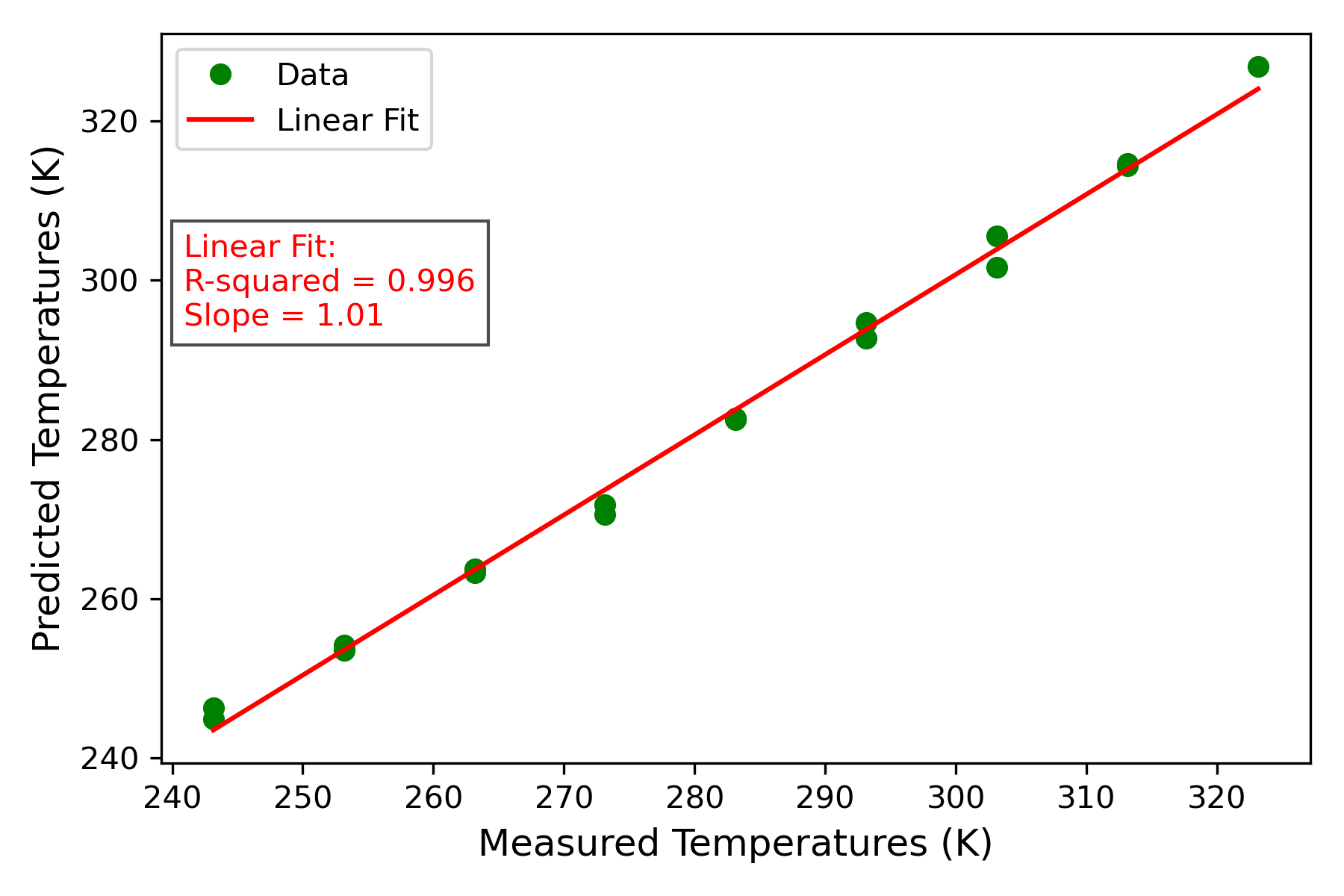
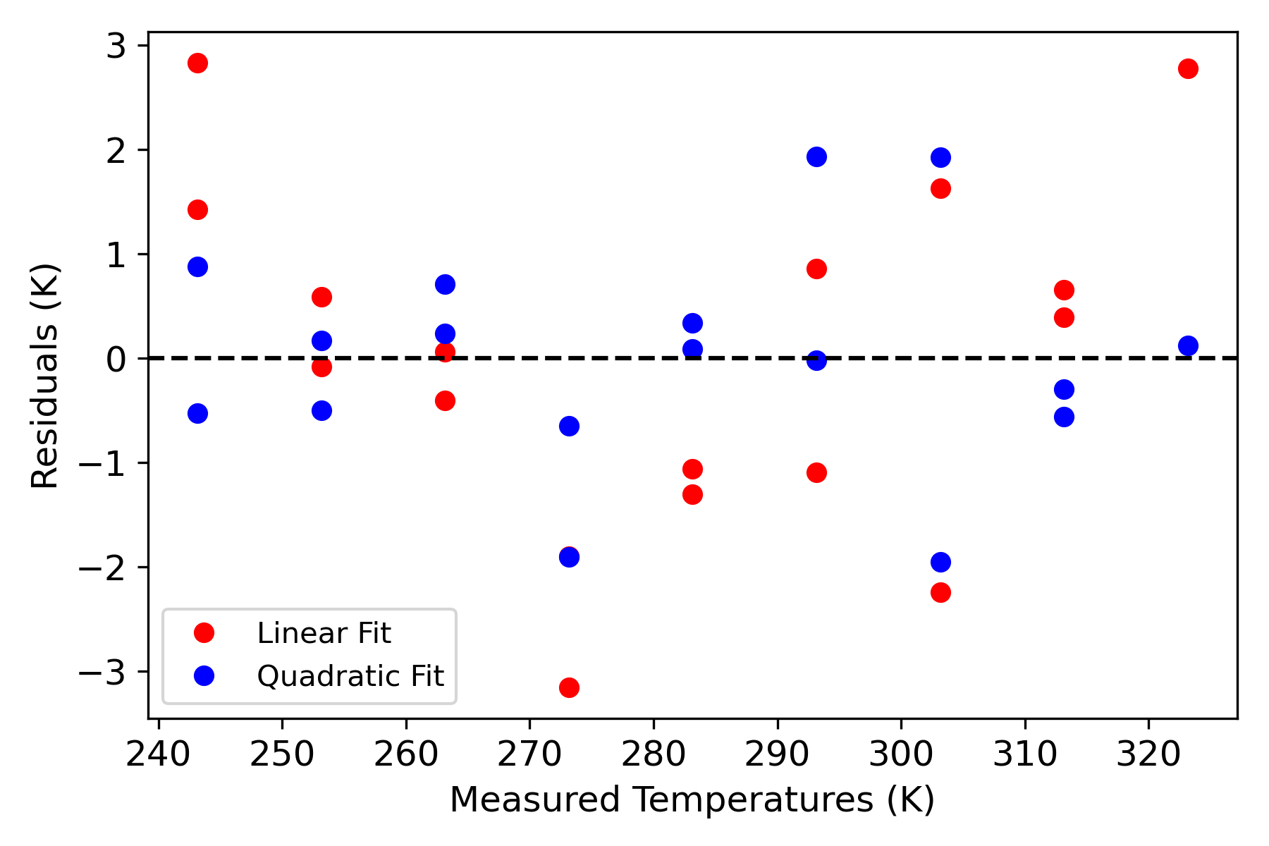
Figure 3: Left: Cycle 2 (243.14 K to 323.15 K) data fit with parameters from Cycle 1 (283.5 K to 323.15 K), showcasing cross-cycle calibration capability. Right: Residuals shown against temperature.

2.4 Estimating temperature using Automatic Peak Detection (AP)

2.4.1 Overview of the Model

The probabilistic model described in the previous section relies heavily on expert knowledge to parameterize the relationship between observed spectra and temperature. It offers a holistic perspective of the entire curve, leveraging its shape and dimensions to accurately determine it’s temperature dependence. In contrast, the auto peak finder method, merely leverages the expert knowledge to posit that changes in peak (or valley) positions are correlated to changes in temperature.

The peak finding algorithm pinpoints the positions of significant peaks by closely scrutinizing the local characteristics of the data. It achieves this by examining the behavior of two neighboring data points surrounding a peak to precisely identify its location. While the probabilistic model provides a comprehensive understanding of the curve’s structure, the peak finding algorithm prioritizes localized features, allowing for efficient (fast) and targeted peak detection within the dataset.

2.4.2 Running the Model

We begin by using the Python library peakutils to identify the indices of the peaks. To facilitate the algorithm we invert the spectra such that valleys appear as peaks.The indices identified by the algorithm as corresponding to peak locations are then sorted according to the corresponding y values (amplitudes). For the highest peak, a window of data points around the peak index is selected. A quadratic function is then fitted to these data points using the method of least squares. The location of the maximum of the fitted quadratic function is taken as the estimated peak location. This process is repeated for the next highest peak, excluding the data points already used for the previous peak(s). The estimated peak locations are stored for further analysis and used to generate training and testing datasets. A linear regression model is then constructed to relate the temperature ($T$) to the peak locations, $P_{1}$ or $P_{2}$:

$$T=\alpha_{0}+\alpha_{1}P$$ (9)

where $\alpha_{0}$ and $\alpha_{1}$ are the coefficients to be determined.

Using the training dataset, which consists of the peak locations and the corresponding temperatures, the linear regression model is trained to determine the values of $\alpha_{0}$, $\alpha_{1}$, and $\alpha_{2}$. After training, the linear regression model predicts temperatures for the testing dataset, and its performance is assessed by comparing these predictions with the actual temperatures, resulting in the calculation of the testing error. Additionally, the model generates temperature predictions for the training dataset, allowing for the computation of the training error. Both the testing and training errors are depicted in Figure  4 and results summarized in Tables 1-3. These results show the peak finder method results in prediction uncertainties that are upto 67$\%$ larger than than the probabilistic model. Post-bias correction the AP model’s prediction uncertainty (2.30 K) is more than double the prediction uncertainty of probabilistic model.

Figure 4: Left : The model was trained on the peak locations extracted from the ODMR spectra of cycle 2 (243.14 K to 323.15 K). Right : Tested on the peak locations from cycle 1 (283.5 K to 323.15 K). The training and testing errors quantify the model’s performance in predicting temperatures from the peak locations.

2.5 Estimating temperature using a data driven approach

2.5.1 Overview of the Model

The proposed methodology adopts a model-free approach known as Principal Component Regression (PCR) to infer temperature from ODMR spectra. The key steps of PCR are: (1) Principal Component Analysis (PCA) [16, 26] for dimensionality reduction and (2) linear regression for establishing the temperature-spectral relationship. This approach contrasts with the model-based approach in that it does not make make any assumptions about the distribution of spectral data nor it’s temperature dependence. It relies entirely on the presented data to learn the relationship between spectra and temperature.

PCA serves as a robust tool for extracting the dominant modes of variation within the spectral dataset. By identifying these principal components (PCs), PCA facilitates dimensionality reduction while preserving essential information concerning temperature-dependent spectral features. Given the potentially high dimensionality of ODMR spectra, PCA is pivotal for capturing pertinent information within a lower-dimensional subspace.

In the PCA step, the modes (principal components) of the data are obtained by solving the eigenvalue problem:

$$CU=US$$ (10)

where $C$ represents the $p\times p$ covariance matrix of the $n\times p$ data matrix $X$, $S$ denotes the $p\times p$ diagonal matrix of eigenvalues, and $U$ is the $p\times p$ matrix whose columns are the eigenvectors of $C$. To reduce dimensionality, the top $k$ eigenvectors corresponding to the largest eigenvalues are selected. For our purposes, $k$ is set to 3, meaning that we choose the top 3 eigenvectors. These eigenvectors form the principal components that capture the most variance in the data. Subsequently, the data are projected onto these principal components using the following equation:

$$Y=(X-\mu)U_{k}$$ (11)

In this equation, $X$ represents the original data matrix, which is first centered by subtracting the mean vector $\mu$. The matrix $U_{k}$ is of size $p\times k$ and contains the top $k$ eigenvectors corresponding to the largest eigenvalues. The projection process involves multiplying the centered data matrix $(X-\mu)$ by $U_{k}$, resulting in a new data matrix $Y$ with dimensions $n\times k$. Here, $n$ is the number of data points and $k=3$ is the number of selected principal components. Each column of $Y$ represents the coordinates of a data point in the 3-dimensional space spanned by the principal components. Following dimensionality reduction via PCA, any form of regression can be employed to predict the temperature $T$ from the projected data $Y$. This is expressed as:

$$T=f(Y,\theta)$$ (12)

where $\theta$ represents the regression parameters. For instance, in linear regression, one fits $T=\varphi Y+\beta$, while in quadratic regression, one fits $T=\psi y^{2}+\varphi y+\beta$, where $y$ denotes the independent variable (i.e., the projected data $Y$). By learning a linear mapping between the reduced-dimensional spectral representation and the temperature values, the regression model provides a straightforward means of temperature inference.

2.5.2 Running the Model

As noted above, the PCR model consists of first applying PCA as a feature identification step, and then applying a linear regression. The method is first trained on a subset of the available data, referred to as the in-sample data. PCA is applied to this in-sample data to identify the principal components. These principal components serve as a reduced-dimensional representation of the spectral features, retaining the essential information related to temperature dependence. Next, linear regression is performed on the projected in-sample data, where the principal component scores are used as input features, and the corresponding temperature values are used as the target variable. This regression learns the linear mapping between the reduced-dimensional spectral representation and the temperature values, effectively establishing the temperature-spectral relationship.

After training the model, it can be effectively applied to out-of-sample data, using the same mean $\mu$ and modes $U$ learned from the in-sample data, as described in equations Eq. (10) and Eq. (11). This out-of-sample data comprises new ODMR spectra that were not included in the initial training set. These out-of-sample spectra undergo identical pre-processing steps, encompassing normalization and projection onto the previously learned principal components. Subsequently, the projected out-of-sample data are input into the trained linear regression model, which then predicts corresponding temperature values based on the learned temperature-spectral relationship. Notably, this prediction step is computationally efficient and can be performed in real-time, rendering the approach highly suitable for practical applications.

The proposed data-driven approach offers a robust and efficient solution for temperature inference from ODMR spectra. By integrating PCA for dimensionality reduction and linear regression for establishing the temperature-spectral relationship, this methodology provides a versatile framework adaptable to various experimental conditions, enabling accurate temperature prediction from ODMR spectra, even for out-of-sample scenarios. As shown in Fig  5 the data driven model readily learns the underlying mapping between temperature and eigenmodes of the PCA, with testing and training errors that are up to $0.67$ K lower than the statistical model. Examination of the top 3 eigenmodes, shown in Fig 6 , reveals that the non-parametric model learns the temperature dependent changes in the spectral lineshape’s moments including changes in peak center, width and amplitude. We note that the non-parametric approach is data hungry, as illustrated in Fig 6, reduction in temperature range degrades the quality of the third mode, returning a mode dominated by random noise. As such the method reports factor of $\approx 10$ increase in prediction errors when tasked with extrapolation beyond the training range (Table 1 ).

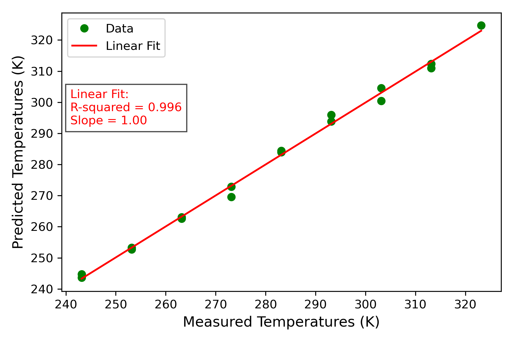
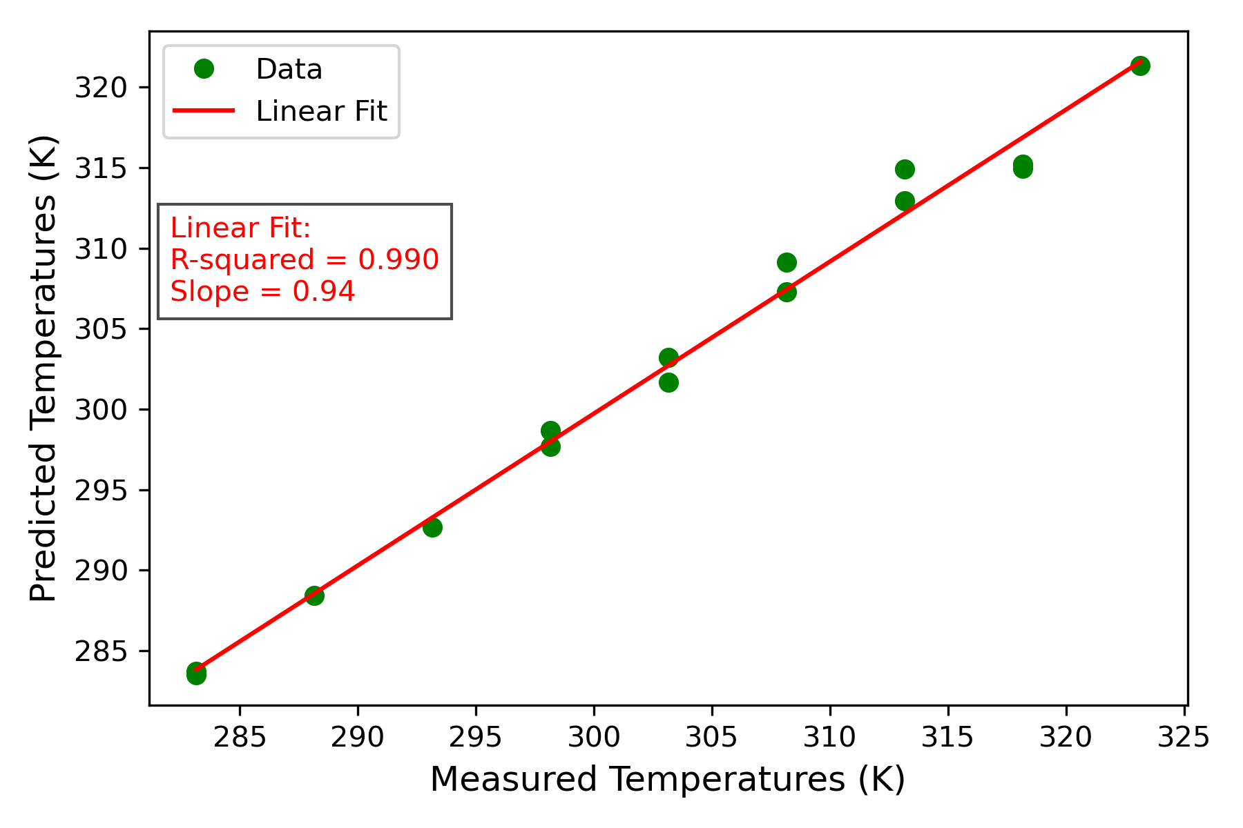
Figure 5: Left: Training Error - Performance of the PCA regression model on cycle 2 (243.14 K to 323.15 K) of the sensor. Right: Testing Error - Evaluation of the PCA regression model’s performance on cycle 1 (283.5 K to 323.15 K) of the same sensor.

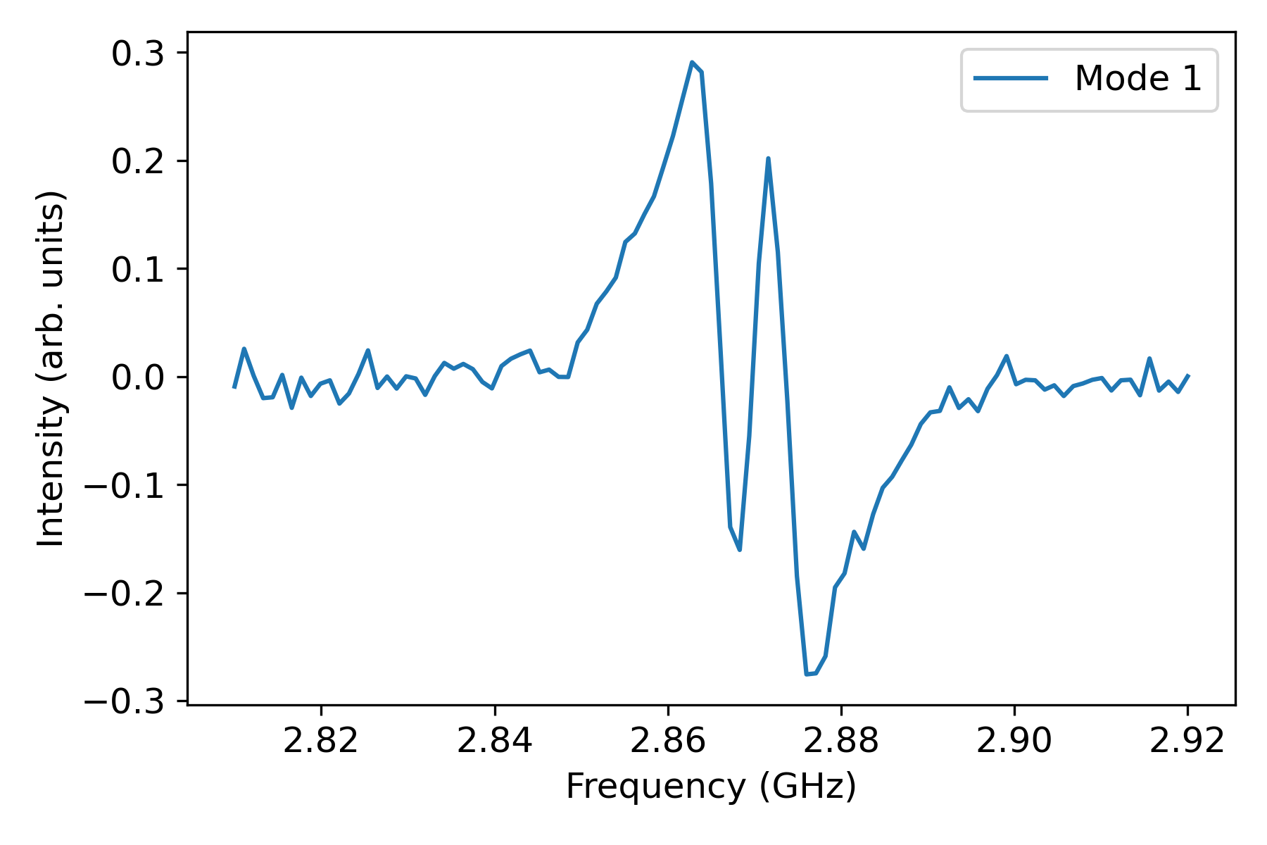
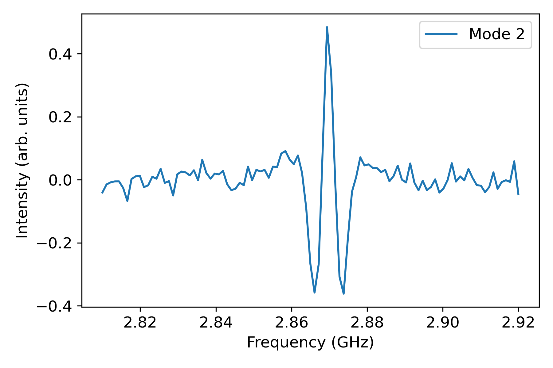
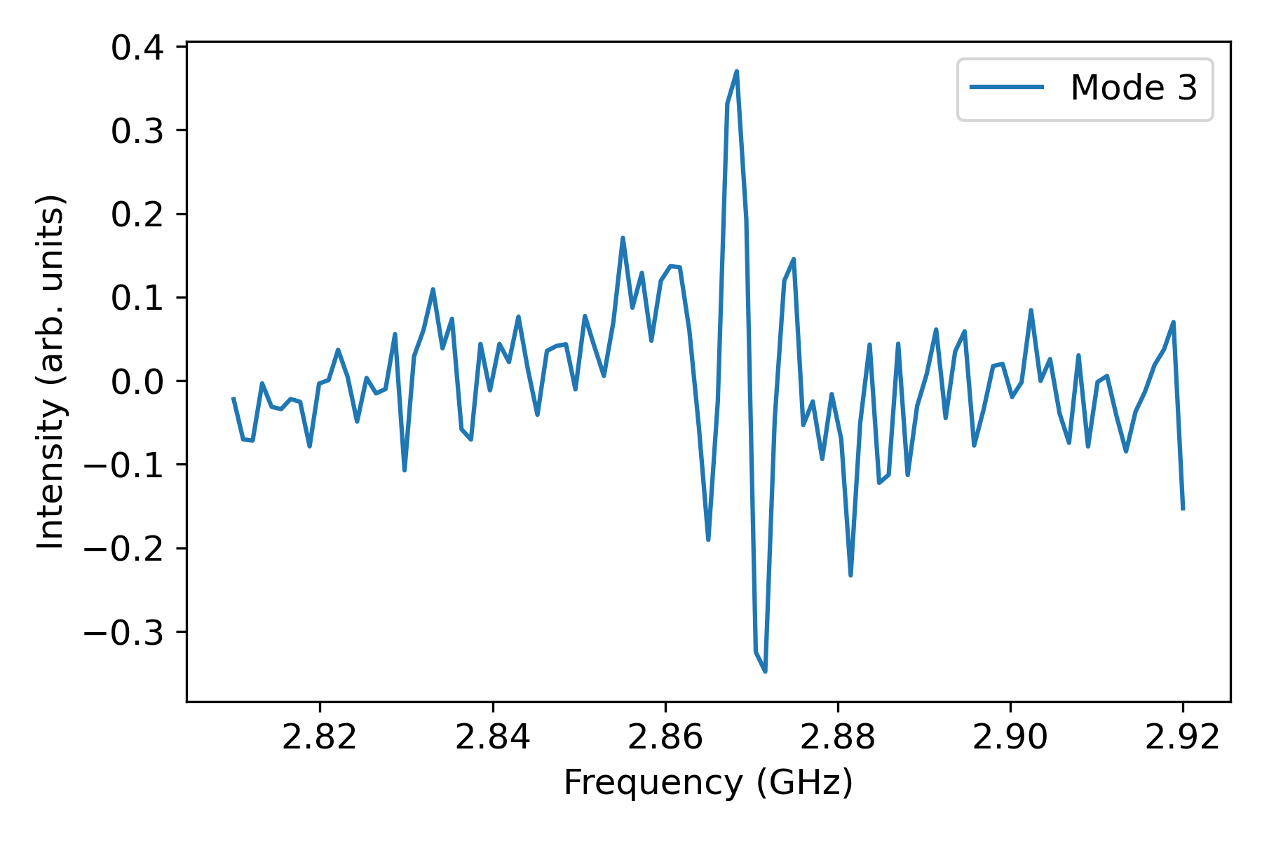
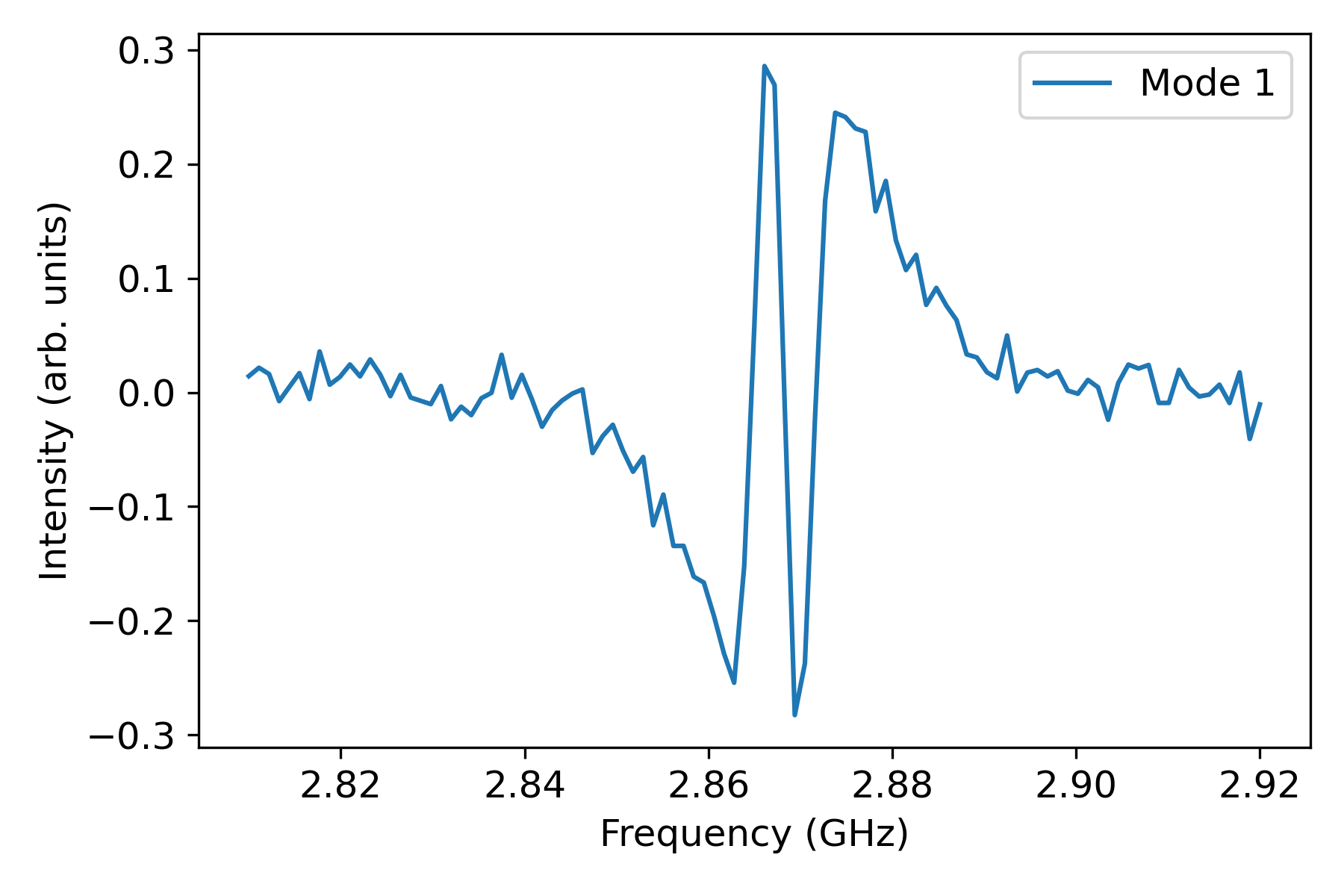
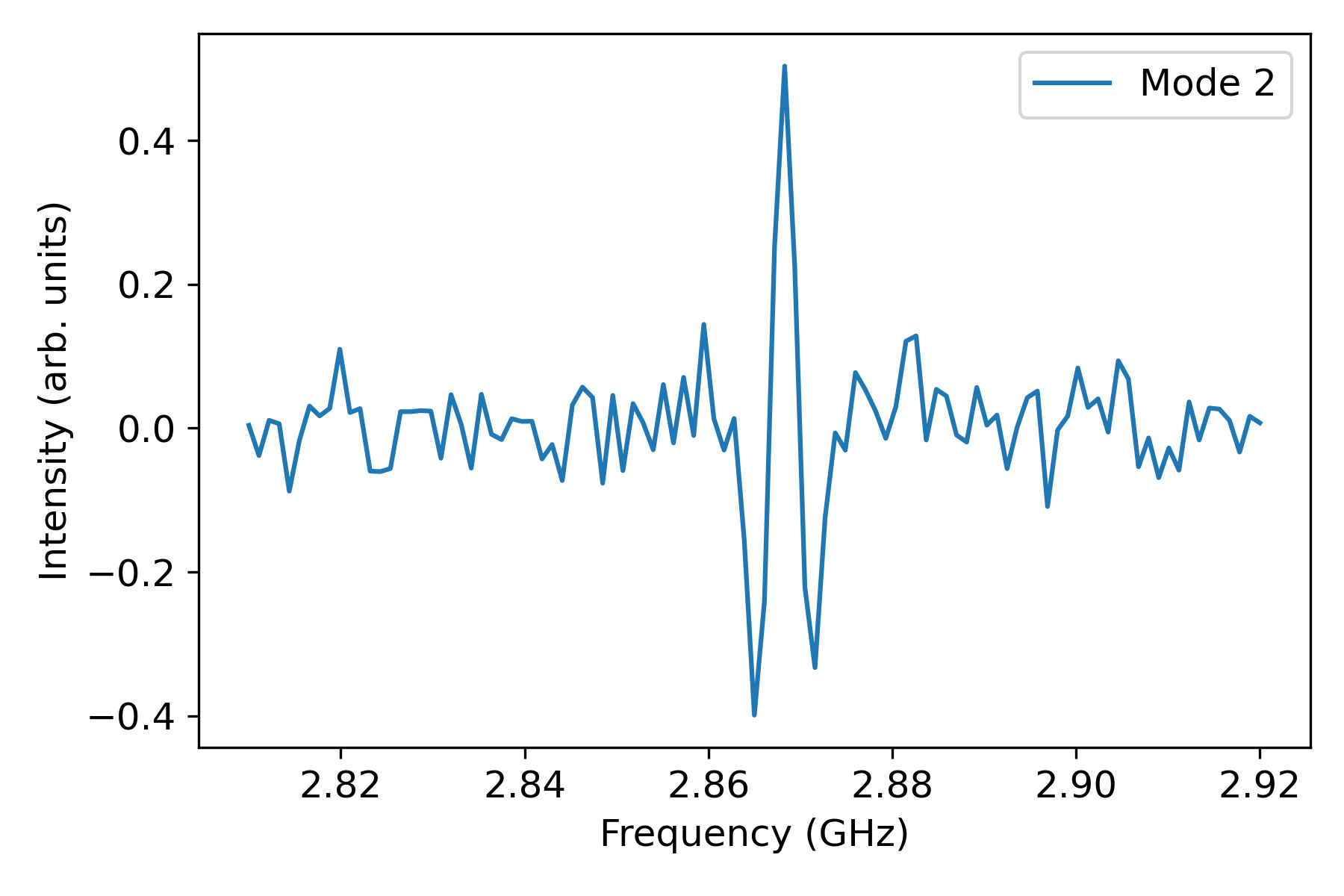
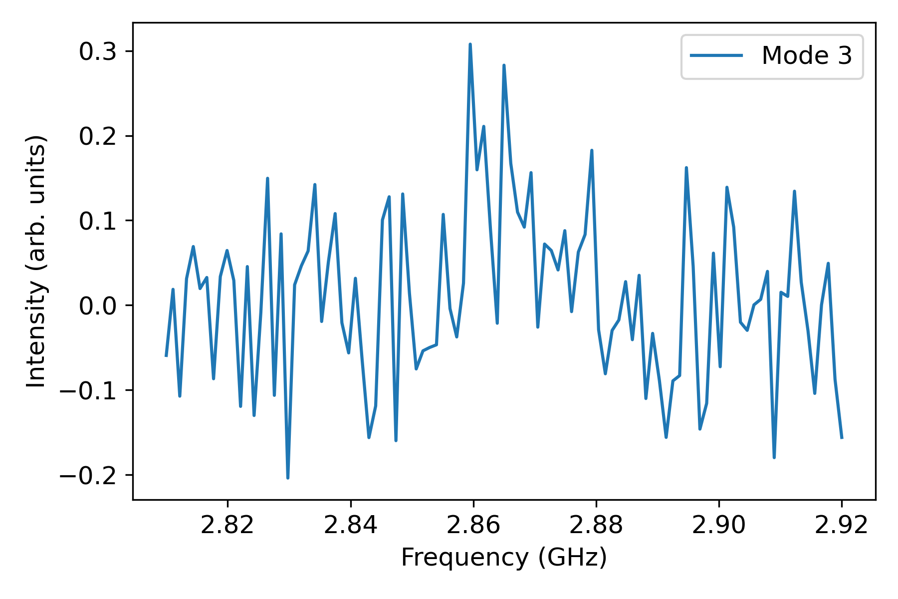
Figure 6: Modes obtained from Principal Component Analysis (PCA) regression modeling for two different temperature ranges. Top: Modes representing the dominant patterns of variation in the data for the temperature range of 243.14 K to 323.15 K. Bottom: Modes capturing the principal components of the data within the narrower temperature range of 283.5 K to 323.15 K. The modes are visualized as spatial patterns, revealing the characteristic features or structures associated with the respective temperature ranges.

2.6 Estimating temperature using Convolutional Neural Network (CNN)

We trained a multi-layer perceptron (MLP) using raw spectroscopic data. The MLP architecture included a flatten layer, two dense layers, and an output layer with ReLU activation functions. We conducted a hyperparameter sweep that systematically varied the hidden layer sizes, learning rates, and weight decay factors. Specifically, we used a learning rate of 0.001, with the first dense layer having 48 nodes, the second dense layer having 20 nodes, and the output layer set to 1. The MLP achieved a testing error of 3.14 K which is considerably larger than other models including the autopeak finder alogrithm. To improve upon MLP’s performance we decided to use a more sophisticated approach: a 1D-Convolutional Neural Network. We employed the Sequential API from Keras as the foundation for developing a Convolutional Neural Network (CNN) specifically tailored for temperature prediction. This model architecture, organized as a sequential stack of layers, is adept at handling sequential data such as the ODMR spectra. It encompasses Convolutional Layers for extracting features, MaxPooling1D Layers for dimension reduction, a Flatten Layer to prepare data for subsequent fully connected layers, Dense Layers for making predictions, and a Dropout Layer for regularization. Crucial hyperparameters, such as filter numbers, kernel size, dense layer units, dropout rate, and learning rate, are meticulously fine-tuned using Keras tuner [27]. The CNN model, compiled with the Adam optimizer [28] and equipped with a loss function for measuring prediction accuracy, dynamically learns pertinent features from the input data, enabling precise temperature forecasts even for unseen data. Through extensive training on the dataset, the CNN model effectively discerns intricate patterns and relationships, culminating in accurate temperature predictions (Figure  7). This process is complemented by the visualization of the hyperparameter sweep all illustrated in Figure 8. This visual exploration allows for fine-tuning critical parameters, ensuring the CNN model attains its lowest validation loss and achieves optimal predictive capability.

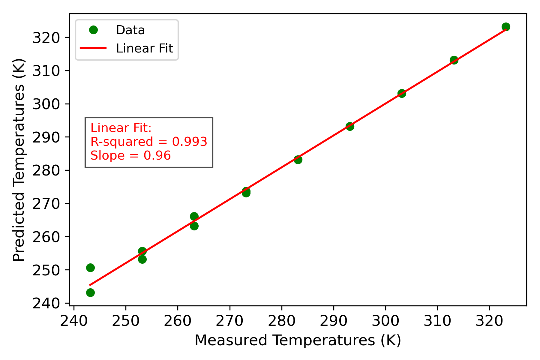
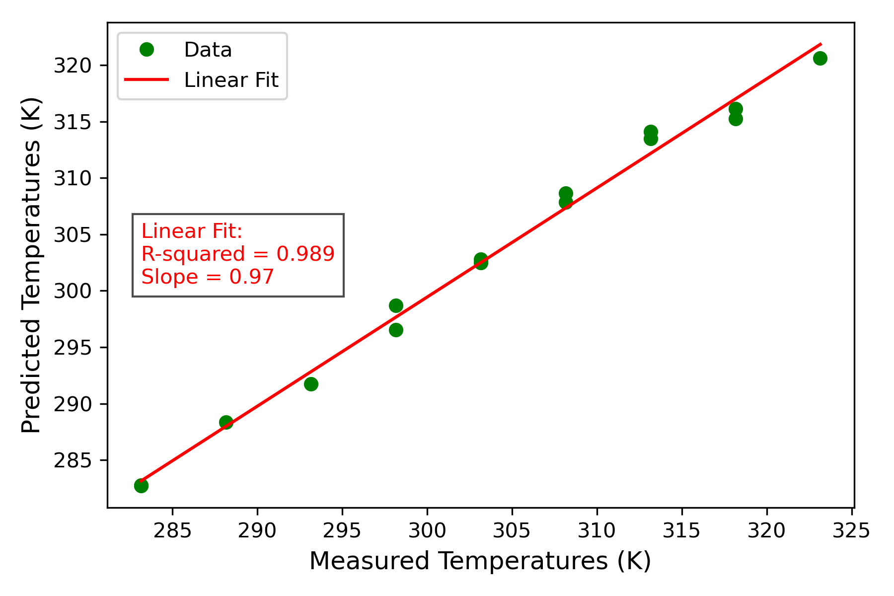
Figure 7: Left: Training error of the CNN model, which was trained on the cycle 2 (243.14 K to 323.15 K) dataset from the sensor. Right: Testing error of the CNN model, which was tested on the cycle 1 (283.5 K to 323.15 K) dataset from the sensor. The plot depicts the discrepancy between the CNN’s predicted temperatures and the actual temperatures. As the CNN iteratively optimizes its parameters, guided by the loss function, it progressively enhances its ability to capture the intricate temperature distributions even in the absence of labeled data.

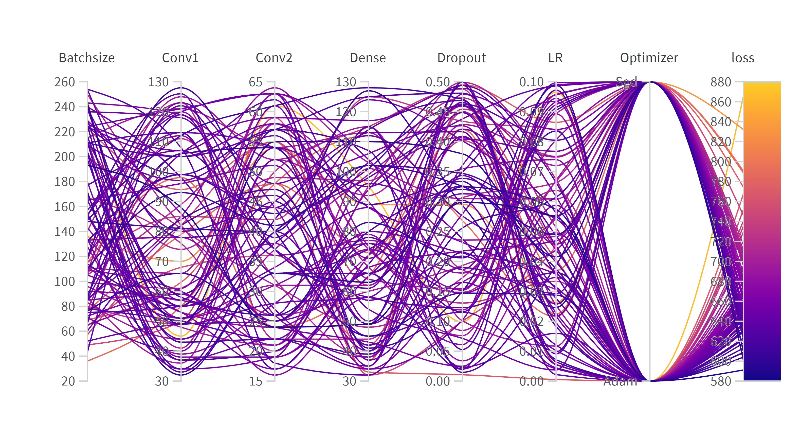
Figure 8: The figure is a visualization of the hyperparameter sweep performed over the sensor data. Curves that are closer in shape to dark purplish correspond to models that yield high performance, with respect to training loss, whereas yellow and orange are sub optimal. Image created using Weights and Biases.[29]. Conv1 and Conv2 refer to the convolutional layers 1 and 2, respectively while LR represents learning rate.

Table 1: Across cycle comparison of RMSE (Kelvin) of our probabilistic model with models based on Automatic Peak-detection (AP), Principal Component Regression (PCR), and 1D Convolutional Neural Networks (CNN).

RMSE (Kelvin)		Expert Knowledge Driven		Data Driven
Training	Testing	Probabilistic Model	AP	PCR	CNN
Cycle2	Cycle1	2.08	2.35	1.42	2.12
Cycle1	Cycle2	1.47	3.14	15.3	18.75

Table 2: In cycle comparison of RMSE (Kelvin) of our probabilistic model with models based on Automatic Peak-detection (AP), Principal Component Regression (PCR), and 1D Convolutional Neural Networks (CNN).

RMSE (Kelvin)		Expert Knowledge Driven		Data Driven
Training	Testing	Probabilistic Model	AP	PCR	CNN
Cycle1	Cycle1	1.9	2.14	1.23	2.16
Cycle2	Cycle2	1.7	2.84	1.59	1.75

Table 3: Comparison of RMSE (Kelvin) of each model followed by a linear or quadratic residual model.

RMSE (Kelvin)		Expert Knowledge Driven		Data Driven
Testing	Polynomial	Probabilistic Model	AP	PCR	CNN
Cycle1	Linear	1.11	2.3	1.16	1.03
Cycle1	Quadratic	1.03	1.9	1.10	0.99
Cycle2	Linear	1.62	2.83	5.65	4.24
Cycle2	Quadratic	1.02	2.30	1.78	1.08

The trained model, corrected for bias, when tested within range outperforms the probabilistic model by 40 mK (Table 3). However when tasked with extrapolation i.e. trained on cycle 1 and tested on cycle 2, the model performs nine times worse than the probabilistic model (see tables 1 and 2 ). This is primarily due to the fact that cycle 2 encompasses a wider range of temperatures that the model has not been exposed to during training, unlike cycle 1. Consequently, the model struggles to generalize to these unseen temperatures, leading to higher prediction errors.

3 Summary

Successful adoption of emerging technologies in sensing, be they photonics or quantum-based, depends on a range of factors including cost, size, weight and power requirements, compatibility with existing infrastructure and workflow, and sensing performance metrics such as resolution and accuracy [4]. In recent years researchers have demonstrated fiberization of photonic and quantum sensors can lead to fit-for-purpose devices that have similar dimensions as legacy sensors addressing an important concern of the user-community [30, 31]. Validating the performance metrics of packaged device including determining uncertainties is the focus of on-going work [4, 32, 30].

In this study we have examined the impact the of inference models on uncertainties of a fiberized NV-diamond based temperature sensor by evaluating the model prediction uncertainties. We have compared the performance of a physics-informed probabilistic model with a conventional peak tracking methodology that draws on minimal domain knowledge, to data-driven models that are agnostic to the device physics. Our results demonstrate that data-driven models are easy to train, generalize well and within the training range, outperform the probabilistic model. However, these models are data hungry and can be sensitive to random measurement noise particularly when the training datasets are small. Furthermore, whilst all models struggle with extrapolation, data-driven models performed worse, resulting in prediction uncertainties that were a factor of $\approx 10$ worse than the probabilistic model.

The unique strengths and weaknesses of the probabilistic and data-driven models opens up new avenue for exploration. The probabilistic model, presents a transparent model that readily provides access to uncertainties in model output. Furthermore, this model can be readily utilized in Kalman filters to enable sensor fusion for sensor network based measurements. In contrast the data-driven models fail to extrapolate beyond the training range, though they outperform probabilistic model when presented with in-range data. These results suggest that hybrid models that weigh outputs of data-driven and probabilistic models may provide the best overall performance.

4 Acknowledgments:

The authors would like to acknowledge AFMETCAL (R24-685-0005) for funding. Shraddha Rajpal and Tyrus Berry would also like to acknowledge support from NSF grant DMS-2006808.

References

- [1] X. Y. Woo, Z. K. Nagy, R. B. Tan, and R. D. Braatz, “Adaptive concentration control of cooling and antisolvent crystallization with laser backscattering measurement,” \JournalTitleCrystal Growth and Design 9, 182–191 (2009).
- [2] R. Price, “The platinum resistance thermometer: a review of its construction and applications,” \JournalTitlePlatinum Metals Review 3, 78–87 (1959).
- [3] G. F. Strouse, “Standard platinum resistance thermometer calibrations from the ar tp to the ag fp,” \JournalTitleNIST Special Publication 250, 1–66 (2008).
- [4] S. Dedyulin, Z. Ahmed, and M. G, “Emerging technologies in the field of thermometry,” \JournalTitleMeasurement Science and Technology 33, 092001 (2022).
- [5] H. Xu, M. Hafezi, J. Fan, et al., “Ultra-sensitive chip-based photonic temperature sensor using ring resonator structures,” \JournalTitleOptics Express 22, 3098–3104 (2014).
- [6] T. P. Purdy, K. E. GRUTTER, K. K. Srinivasan, and J. M. Taylor, “Quantum correlations from a room-temperature optomechanical cavity,” \JournalTitleScience 356, 1265–1268 (2017).
- [7] J. F. Qu, S. P. Benz, H. Rogalla, et al., “Johnson noise thermometry,” \JournalTitleMeas. Sci. Technol. 30, 112001 (2019).
- [8] J. R. Maze, P. L. Stanwix, J. S. Hodges, et al., “Nanoscale magnetic sensing with an individual electronic spin in diamond,” \JournalTitleNature 455, 644–647 (2008).
- [9] F. Dolde, H. Fedder, M. W. Doherty, et al., “Electric-field sensing using single diamond spins,” \JournalTitleNature Physics 7, 459–463 (2011).
- [10] P. Neumann, I. Jakobi, F. Dolde, et al., “High-precision nanoscale temperature sensing using single defects in diamond,” \JournalTitleNano letters 13, 2738–2742 (2013).
- [11] D. M. David M. Toyli, C. F. de las Casas, D. J. Christle, and D. D. Awschalom, “Fluorescence thermometry enhanced by the quantum coherence of single spins in diamond,” \JournalTitlePNAS 110, 8417–8421 (2013).
- [12] G. Kucsko, P. C. Maurer, N. Y. Yao, et al., “Nanometre-scale thermometry in a living cell,” \JournalTitleNature 500, 54–58 (2013).
- [13] S.-C. Zhang, Y. Dong, B. Du, et al., “A robust fiber-based quantum thermometer coupled with nitrogen-vacancy centers,” \JournalTitleReview of Scientific Instruments 92 (2021).
- [14] I. Fedotov, S. Blakley, E. Serebryannikov, et al., “Fiber-based thermometry using optically detected magnetic resonance,” \JournalTitleApplied Physics Letters 105, 261109 (2014).
- [15] M. Fujiwara and Y. Shikano, “Diamond quantum thermometry: from foundations to applications,” \JournalTitleNanotechnology 32, 482002 (2021).
- [16] W. F. Massy, “Principal components regression in exploratory statistical research,” \JournalTitleJournal of the American Statistical Association 60, 234–256 (1965).
- [17] K. O’shea and R. Nash, “An introduction to convolutional neural networks,” \JournalTitlearXiv preprint arXiv:1511.08458 (2015).
- [18] M. W. Doherty, N. B. Manson, P. Delaney, et al., “The nitrogen-vacancy colour centre in diamond,” \JournalTitlePhysics Reports 528, 1–45 (2013).
- [19] P. Rembold, N. Oshnik, M. M. Müller, et al., “Introduction to quantum optimal control for quantum sensing with nitrogen-vacancy centers in diamond,” \JournalTitleAVS Quantum Science 2 (2020).
- [20] T. Griffiths and A. Yuille, “A primer on probabilistic inference,” \JournalTitleThe probabilistic mind: Prospects for Bayesian cognitive science pp. 33–57 (2008).
- [21] M. J. Powell, “An efficient method for finding the minimum of a function of several variables without calculating derivatives,” \JournalTitleThe computer journal 7, 155–162 (1964).
- [22] J. Brewer, “Kronecker products and matrix calculus in system theory,” \JournalTitleIEEE Transactions on circuits and systems 25, 772–781 (1978).
- [23] G. Strang, Linear algebra and learning from data (SIAM, 2019).
- [24] P. Goldsborough, “A tour of tensorflow,” \JournalTitlearXiv preprint arXiv:1610.01178 (2016).
- [25] P. Virtanen, R. Gommers, T. E. Oliphant, et al., “Scipy 1.0: fundamental algorithms for scientific computing in python,” \JournalTitleNature methods 17, 261–272 (2020).
- [26] J. R. Beattie and F. W. Esmonde-White, “Exploration of principal component analysis: deriving principal component analysis visually using spectra,” \JournalTitleApplied Spectroscopy 75, 361–375 (2021).
- [27] T. O’Malley, E. Bursztein, J. Long, et al., “Kerastuner,” https://github.com/keras-team/keras-tuner (2019).
- [28] D. P. Kingma and J. Ba, “Adam: A method for stochastic optimization,” \JournalTitlearXiv preprint arXiv:1412.6980 (2014).
- [29] R. Guha, D. T. Stanton, and P. C. Jurs, “Interpreting computational neural network quantitative structure- activity relationship models: A detailed interpretation of the weights and biases,” \JournalTitleJournal of chemical information and modeling 45, 1109–1121 (2005).
- [30] S. Janz, S. Dedyulin, D. X. Xu, et al., “Measurement accuracy in silicon photonic ring resonator thermometers: identifying and mitigating intrinsic impairments,” \JournalTitleOpt. Express 32, 551–575 (2024).
- [31] Y. Li, F. A. Gerritsma, S. Kurdi, et al., “A fiber-coupled scanning magnetometer with nitrogen-vacancy spins in a diamond nanobeam,” \JournalTitleACS Photonics 10, 1859–1865 (2023).
- [32] M. R. Hartings, N. J. Castro, K. Gill, and Z. Ahmed, “A photonic ph sensor based on photothermal spectroscopy,” \JournalTitleSensors and Actuators B: Chemical 301, 127076 (2019).