Enumerating Minimal Unsatisfiable Cores of LTLf formulas
Abstract
Linear Temporal Logic over finite traces (LTL) is a widely used formalism with applications in AI, process mining, model checking, and more. The primary reasoning task for LTLf is satisfiability checking; yet, the recent focus on explainable AI has increased interest in analyzing inconsistent formulas, making the enumeration of minimal explanations for infeasibility a relevant task also for LTL. This paper introduces a novel technique for enumerating minimal unsatisfiable cores (MUCs) of an LTL specification. The main idea is to encode a LTL formula into an Answer Set Programming (ASP) specification, such that the minimal unsatisfiable subsets (MUSes) of the ASP program directly correspond to the MUCs of the original LTL specification. Leveraging recent advancements in ASP solving yields a MUC enumerator achieving good performance in experiments conducted on established benchmarks from the literature.
Introduction
Linear temporal logic over finite traces (LTL) (De Giacomo and Vardi 2013) is a simple, yet powerful language for expressing and reasoning about temporal specifications, that is known to be particularly well-suited for applications in Artificial Intelligence (AI) (Bacchus and Kabanza 1998; Calvanese, De Giacomo, and Vardi 2002; De Giacomo et al. 2016; De Giacomo and Vardi 1999).
Perhaps its most widely recognised use to-date is as the logic underlying temporal process modelling languages such as Declare (Pesic, Schonenberg, and van der Aalst 2007). Very briefly, a Declare specification is a set of contraints on the potential evolution of a process, which is expressed through a syntactic variant of a subclass of LTL formulas. The full specification can thus be seen as a conjunction of LTL formulas. As specifications become bigger—specially when they are automatically mined from trace logs (Di Ciccio and Montali 2022), it is not uncommon to encounter inconsistencies (i.e., business process models which are intrinsically contradictory) or other errors.
To understand and correct these errors, it is thus important to highlight the sets of formulas in the specification that are responsible for them (Niu et al. 2023; Roveri et al. 2024). Specifically, we are interested in computing the minimal unsatisfiable cores (MUCs): subset-minimal subsets of formulas (from the original specification) that are collectively inconsistent (Liffiton et al. 2016; Niu et al. 2023; Roveri et al. 2024). These can be seen as the prime causes of the error. Notably, a single specification can yield multiple MUCs of varying sizes, depending on the specific constraints involved. Exploring more than one MUC can be crucial for analyzing and understanding the causes of incoherence (as recognized in explainable AI (Miller 2019; Audemard, Koriche, and Marquis 2020)). Thus, a system capable of efficiently enumerating MUCs would be of significant value.
A similar problem has been studied in the field of answer set programming (ASP) (Brewka, Eiter, and Truszczynski 2011; Gelfond and Lifschitz 1991), where the goal is to find minimal unsatisfiable subsets (MUS) of atoms that make an ASP program incoherent (Brewka, Thimm, and Ulbricht 2019; Mencía and Marques-Silva 2020; Alviano et al. 2023). In recent years, efficient implementations of MUS enumerators have been presented (Alviano et al. 2023).
Our goal in this paper is to take advantage of both the declarativity of tha ASP language and the efficiency of ASP systems to also enumerate MUCs of LTL formulas. Hence, we present a new transformation which constructs, given a set of LTL formulas, an ASP program whose MUSes are in a biunivocal corrispondence with the MUCs of the original specification. Importantly, although we base our reduction on a well-known encoding of LTL bounded satisfiability (Fionda and Greco 2018; Fionda, Ielo, and Ricca 2024), the idea is general enough to be applicable to other decision procedures, as long as it can be expressed in ASP. To improve its efficiency, our enumerator checks for unsatisfiability iteratively by considering traces of increasing length based on a progression strategy (Morgado et al. 2013). To the best of our knowledge, we provide the first MUC enumerator for LTL.
We empirically compared our implementation with existing systems designed to produce only one MUC (or just one potentially non-minimal unsatisfiable core) (Niu et al. 2023; Roveri et al. 2024) and observed that our system—despite being more general—is competitive against those on established benchmarks from the literature. Importantly, MUC enumeration is very efficient as well.
Related Work
The task of computing MUCs has been considered, under different names, for several representation languages including propositional logic (Liffiton and Sakallah 2008), constraint satisfaction problems (Mencía and Marques-Silva 2014), databases (Meliou, Roy, and Suciu 2014), description logics (Schlobach and Cornet 2003), and ASP (Alviano et al. 2023) among many others. For a general overview of the task and known approaches to solve it, see (Peñaloza 2020).
Although the task was briefly studied for LTL (over infinite traces) in (Baader and Peñaloza 2010), it was only recently considered for the specific case of LTL (Niu et al. 2023; Roveri et al. 2024). Interestingly, for LTL the focus has been only on computing one (potentially non-minimal) unsatisfiable core. To our knowledge, we are the first to propose a full-fletched LTL MUC enumerator.
The idea of using a highly optimised reasoner from one language to enumerate MUCs from another one was already considered, first exploiting SAT solvers (Sebastiani and Vescovi 2009) and later on using ASP solvers (Peñaloza and Ricca 2022). Our approach falls into the latter class. Our reduction to ASP is inspired on the automata-based satisfiability procedure, previously used for SAT-based satisfiability checking (Fionda and Greco 2018; Li et al. 2020a), alongside an incremental approach that verifies the (non-)existence of models up to a certain length.
Preliminaries
We briefly recap required notions of Linear Temporal Logic over Finite Traces (LTL) (De Giacomo and Vardi 2013) and Answer Set Programming (ASP) (Brewka, Eiter, and Truszczynski 2011).
Answer Set Programming
Syntax and semantics.
A term is either a variable or a constant, where variables are alphanumeric strings starting with uppercase letter, while constants are either integer number or alphanumeric string starting with lowercase letter. An atom is an expression of the form where is a predicate of ariety and are terms; it is ground if all its terms are constants. We say that an atom has signature . An atom matches a signature if . A literal is either an atom or its negation , where denotes the negation as failure. A literal is said to be negative if it is of the form , otherwise it is positive. For a literal , denotes the complement of . More precisely, if , otherwise . A normal rule is an expression of the form where is an atom referred to as head, denoted by , that can also be omitted, , and is a conjunction of literals referred to as body, denoted by . In particular a normal rule is said to be a constraint if its head is omitted, while it is said to be a fact if . A normal rule is safe if each variable appears at least in one positive literal in the body of . A program is a finite set of safe normal rules. In what follows we will use also choice rules, which abbreviate complex expressions (Calimeri et al. 2020). A choice element is of the form , where is an atom, and is a conjunction of literals. A choice rule is an expression of the form , which is a shorthand for the set of normal rules ; , for each where are of the form and is a fresh atom not appearing anywhere else.
Given a program , the Herbrand Universe of , , denotes the set of constants that appear in , while the Herbrand Base, , denotes the set of ground atoms obtained from predicates in and constants in . Given a program , and , denotes the set of ground instantiations of obtained by replacing variables in with constants in . Given a program , denotes the union of ground instantiations of rules in . An interpretation is a set of atoms. Given an interpretation , a positive (resp. negative) literal is true w.r.t. if (resp. ); otherwise it is false. A conjunction of literal is true w.r.t if all its literals are true w.r.t. . An interpretation is a model of if for every rule , is true whenever is true. Given a program and an interpretation , the (Gelfond-Lifschitz) reduct (Gelfond and Lifschitz 1991), denoted by , is defined as the set of rules obtained from by deleting those rules whose body is false w.r.t and removing all negative literals that are true w.r.t. from the body of remaining rules. Given a program , and a model , then is also a answer set of if no such exists such that is a model of . For a program , let denotes the set of answer sets of , then is said to be coherent if , otherwise it is incoherent. Given an answer set and a signature , the projection of on is the set .
MUSes and MSMs
Consider a program and a set of objective atoms . For , we denote by the program obtained from by adding a choice rule over atoms in (i.e. ) and a set of constraints of the form , for every . Intuitively, denotes an augmentation of the program in which the objective atoms can be arbitrarily choosen (i.e. either as true or false) but the atoms in are enforced to be true.
An unsatisfiable subset for w.r.t. the set of objective atoms is a set of atoms such that is incoherent. denotes the set of unsatisfiable subsets of w.r.t. . An unsastisfiable subset is a minimal unsatisfiable subset (MUS) of w.r.t. iff for every , . Analogously, an answet set is a minimal stable model (MSM) of w.r.t. the set of objective atoms if there is no answer set with .
Linear Temporal Logic over Finite Traces
Linear Temporal Logic (LTL) (Pnueli 1977) is an extension of propositional logic which allows to reason over infinite sequences of propositional interpretations or traces. LTL (De Giacomo and Vardi 2013) is a variant of this logic that considers only finite traces. Let be a finite set of propositional symbols. The class of LTL formulas over is defined according to the grammar
where . A formula is in conjunctive form if it is expressed as a conjunction of formulas. In this case, we often represent a formula as the set of its conjuncts; i.e., the formula is expressed by the set .
A state is any subset of ; a trace is a finite sequence of states; in this case, the trace has length . The -th state of the trace is denoted by The satisfaction relation is defined recursively over the structure of . Let be a trace and . We say that satisfies at time , denoted by iff:
-
•
iff ;
-
•
;
-
•
iff and ;
-
•
iff and ; and
-
•
if there exists s.t. and for all , .
The trace is a model of (denoted by ) whenever . The satisfiability problem is the problem of deciding whether a formula admits a model; i.e., if there exists such that . LTL satisfiability is well-known to be PSpace-complete (De Giacomo and Vardi 2013).
Given an unsatisfiable formula in conjunctive form, a minimal unsatisfiable core (MUC) of is an unsatisfiable formula which is minimal (w.r.t. set inclusion); i.e., removing any conjunct from yields a satisfiable formula (Niu et al. 2023). Complexity-wise, it is known that a single formula may have exponentially many MUCs, but computing one MUC requires only polynomial space; just as deciding satisfiability (Peñaloza 2019, 2020).
Method
Technique approach proposed in this paper relies on leveraging ASP minimal unsatisfiable sets (MUSes) enumeration algorithms to generate a sequence of candidate minimal unsatisfible cores (MUCs) for an LTL formula. In order to put in place such approach, a formal connection between these objects must be established. In this section, we introduce the notion of probe and -MUC to investigate this relationship. A probe is an abstraction over the class of logic programs with suitable properties to apply the approach herein presented; -MUCs are a relaxation wrt model length of the concept of MUC, which reveals to be more suitable for ASP-based reasoning.
MUS and Probes
In the rest of the paper we adopt the notation introduced in in (Niu et al. 2023). Let be a formula in conjunctive form, where is a conjunct of . With a slight abuse of notation, we will identify with the set of its conjuncts.
Our first assumption is that there exists an uniform way to encode LTL formulae in conjunctive normal form into logic programs. In particular, we are interested in encodings where original conjuncts of can be told apart by means of special atoms. More formally:
Definition 1 (Reification Function).
A reification function for a formula is a function that maps into a logic program whose Herbrand base contains an atom for each . We denote the set of atoms matching signature by .
Each subset uniquely identifies the set of conjuncts . Therefore, we denote by and by .
Reification functions enable to encode LTL formulae into logic programs. Since in this paper we are concerned with notions of satisfiability, unsatisfiability wrt subset minimality of LTL formulae, among all possible reification functions, we are interested in ones that preserve as much information about these properties. In particular, we introduce the notion of probe.
Definition 2 (-Probe).
Let . A reification function is a probe of depth (or -probe for short) for if for each set it holds that admits a model of length at most if and only if there exists an answer set of such that .
There exist multiple ASP encodings that satisfy the definition of probe. Intuitively, one can obtain a probe by adapting any ASP encoding for bounded LTL satisfiability (Fionda, Ielo, and Ricca 2024; Fionda and Greco 2018). Section A concrete example of probe features an extended and detailed example. Here, we focus on how probes relate to MUCs of .
Lemma 3.
Let be a probe of depth for . Let be a minimal unsatisfiable subset of wrt the objective atoms . Then is either an MUC of or it is satisfiable but its shortest satisficing trace has length greater than .
Proof.
Assume is a minimal unsatisfiable subset wrt . Then, all its (proper) subsets can be extended to answer sets — thus, interpreting them as formulae yields an LTL formula that admits a model of length at most , by Definition 2. Hence, all proper subsets of are satisfiable, while itself is either unsatisfiable or its shortest model trace has a length greater than . In the former case, it matches the definition of MUC. ∎
We provide an example.
Example 4.
Consider the formula . This formula has a unique MUC, namely . If we consider a probe , it has two MUSes, namely , since these formulae do not admit models of length at most 3. If we consider instead probes of depth at least 5, it is now possible to detect the MUC through the (unique) MUS
Formulae exhibiting the property shown in the statement of Lemma 3 are the key objects which allow us to levarage MUS enumeration to enumerate MUCs. Thus, we introduce a definition.
Definition 5 (-bound MUC).
Let . A -bound MUC (or -MUC) for the formula is a minimal subset of that does not admit a model of length at most . We denote by the set of all -MUCs for a formula .
Lemma 6.
Let . If is unsatisfiable, then is a MUC for .
Proof.
Follows from the fact that since , it means that any proper subset of admits a model of length at most , hence it satisfiable. If is also unsatisfiable, it matches the definition of MUC. ∎
We re-state Lemma 3 adopting the new definition:
Lemma 7.
Let be a formula, . is a minimal unsatisfiable subset of the -probe if and only if is a -MUC for .
Example 4 highlights an interesting property. The probe at depth yields two (singleton) MUSes, that intepreted as formulae indeed do not admit models of length at most . However, increasing the probe depth to , yields a single MUS, since the MUSes (of the previous probe) are actually both satisfiable if we consider models of length at most , but still (jointly) unsatisfiable considering models of length at most . Intuitively, this makes the probe at depth more effective, since it allows to discard MUSes that won’t lead to a MUC.
In this regard, with the aim of enumerating MUCs, the most interesting probes would be the ones that allow to detect all MUCs with no false positives. More formally, the most effective probe is a probe at a depth such that for each it holds if is an MUS in a -probe, it will also be an MUS in the -probe. We provide an argument to show that such a probe depth exists.
If , can have at most MUCs. Let be the least integer such that any satisfiable subset of admits a model of length at most . We refer to as the completeness threshold for , and probes of depth greater or equal to as complete probes.
This leads us to the following theorem, which establishes a bijection between MUSes of complete probes and MUCs of :
Theorem 8.
Let be a complete probe for . Then is an MUS of wrt if and only if is a MUC of .
Proof.
Let be an MUS of with respect to . By Lemma 7 is a -MUC, thus it is either unsatisfiable (hence it is a MUC); or satisfiable with a satisficing trace with length greater than — in this latter case, would not be a complete probe. Hence, must be a MUC for . Let be an MUC of . Without loss of generality, we can assume . All its proper subsets — which denotes the LTL formula obtained by removing from the -th conjunct — are satisfiable. Since is a complete probe, for each there exists an answer set of that extends , but there exists no answer set that extends . Since , this shows that is an MUS for wrt . ∎
Theorem 8 characterizes MUCs of as MUSes of complete probes for . From the standard automata-based procedure for deciding satisfiability in LTL (De Giacomo and Vardi 2013; Maggi, Montali, and Peñaloza 2020) it follows that every satisfiable formula has a model of length at most where is the number of subformulas of . Indeed, completeness threshold is bounded above by the upper bound on model length of (due to monotonicity of LTL wrt conjunction — adding a conjunct can only increase the length of the shortest model). However, in practice, it can be much smaller, as we will see in the experiments section.
MUC enumeration by MUS enumeration
Applying Theorem 8 we can enumerate MUCs of by enumerating MUSes of a complete probe for . In general, computing the completeness threshold for is not feasible. However, by Lemma 6, we also know that some -MUCs, with could also be MUCs. These results suggest two anytime algorithms that could be useful in the realm of LTL MUC enumeration: (i) an algorithm (cfr. Algorithm 1) that computes all MUCs among the -MUCs for a given and (ii) an iterative deepening variant of Algorithm 1 (cfr. Algorithm 2) which expands the probe depth whenever a -MUC reveals not to be unsatisfiable. Algorithm 1 and 2 provide pseudo-code for such approaches. Both algorithms make use of the subroutines probe, enumerate_mus, to_formula, check_satisfiability, that are explained next.
- probe
-
builds the logic program from which we will extract -MUCs. This is the counterpart of .
- enumerate_mus()
-
invokes an ASP solver to extract MUSes of the probe wrt the objective atoms ;
- to_formula
-
given an MUS of , rebuilds the LTL formula ;
- check_satisfiability()
-
determines wheter an LTL formula is satisfiable or not; if is satisfiable, returns the length of a satisficing trace; otherwise, it returns 0;
We remark both algorithms are compatible with any ASP solver that implements MUS enumeration (that is, an implementation of the procedure enumerate_mus) and (complete) LTL solvers that can (i) provide a satisficing trace length for satisfiable formulae (ii) prove unsatisfiability (that is, an implementation of the procedure check_satisfiability).
Algorithm 1 is straightforward. We enumerate MUSes of a -probe, which yields a sequence of -MUCs. Each -MUC is a candidate MUC for , that can be certified or disproved by a call to an LTL satisfiability oracle. Following such a call, we discard false positives candidate (that is, -MUCs that are actually satisfiable) as we meet them. This approach does not enable to detect all MUCs, unless . Conjuncts whose shortest model has length greater than will be discarded.
Algorithm 2 extends Algorithm 1. Whenever we encounter a false positive -MUC , this is a witness of the fact the current is below the completeness threshold for . Thus, we increase according to the length of the model that satisfies . Since is finite, will eventually converge to . At that point, all -MUCs of the -probe result in MUCs for .
A concrete example of probe
Probes can be obtained with slight modifications from any ASP encoding to perform bounded satisfiability of LTL formulae. In this section, we show how to obtain a probe from the encoding proposed by (Fionda, Ielo, and Ricca 2024), which repurposes to ASP the SAT-based approach presented in (Fionda and Greco 2018). This will also be the probe we use in the experimental section. In rest of the section, we will provide ASP encoding using the clingo input language, for further detail we refer the reader to (Gebser et al. 2019).
We start by a brief recap of the ASP approach to bounded satisfiability (Fionda, Ielo, and Ricca 2024), then show how the encoding can be seamlessy adapted into a probe.
Encoding formulae.
The starting point is to encode an LTL formula into a set of facts. Each subformula of is assigned an unique integer identifier. This identifier is used as a term in the predicates , , , , and to reify the syntax tree of into a directed acyclic graph.
Example 9.
As an example, consider the formula with two conjuncts is encoded through the facts:
conjunction(0, 1).  conjunction(0, 2).
conjunction(1, 3).  conjunction(1, 4).
atom(3, a).  negate(4, 5).  atom(5, b).
until(2, 6, 5).  atom(6, c).
root(0).
Additionally, the atom encodes that is the root node of the formula . Without loss of generality, we can assume that the root node is always identified by 0. We denote by the set of facts that encode the formula .
Encoding LTL semantics.
The semantics of LTL temporal operators can be encoded into a recursive Datalog program. The logic program below, described more in-depth in (Fionda, Ielo, and Ricca 2024), adapts the SAT-based approach described in (Fionda and Greco 2018).
holds(T,X) :- trace(T,A), atom(X,A).
holds(T,X) :- holds(T+1,F),
  next(X,F), time(T+1).

holds(T,X) :- until(X,LHS,RHS),
  holds(T,RHS).

holds(T,X) :- holds(T,LHS), holds(T+1,X),
  until(X,LHS,RHS).

holds(T,X) :- conjunction(X,_), time(T),
  holds(T,F): conjunction(X,F).

holds(T,X) :- negate(X,F),
  not holds(T,F), time(T)
The predicate is used to encode a trace. In particular, an atom models that . We denote by the set of facts . The logic program admits a unique stable model , such that if and only if .
Encoding LTL bounded satisfiabilty.
The logic program can be used to evaluate whether , where and are suitably encoded into facts. This is straightforwardly adapted into a bounded satisfiability encoding , by replacing the set of facts encoding a specific trace with the following choice rule to :
time(0..k-1).
{ trace(T,A): atom(_,A) } :- time(T).

:- root(X), not holds(X,0).
In a typical guess & check approach, the above choice rule generate the search space of possible satisficing traces for — replacing a set of facts that encode a specific trace .
The constraint discards trace that are not models of . Thus, answer sets of are in one-to-one correspondance with traces of length at most that are models of . Note that is an input constant to the ASP grounder.
The probe.
The above program encodes whether admits a model of length up to . In order to comply with definition of probe (i.e. Definition 2), we require that there exists admits an answer set for each subset of that admits a model of length up to . This is obtained by replacing each fact of the form , where is an identifier of a most immediate subformula of , with a rule of the form , as well as the choice rule .
conjunction(1, 3).  conjunction(1, 4).
atom(3, a).  negate(4, 5).  atom(5, b).
until(2, 6, 5).  atom(6, c).
root(0).

conjunction(0,1) :- phi(0). {phi(0)}.
conjunction(0,2) :- phi(1). {phi(1)}.
As we can see, the only affected rules are the conjunction facts at the root level. Intuitively, the additional choice rule over atoms enables or disables conjuncts of . This is reminiscent of how logic programs under stable model semantics are annotated to exploit MUS enumeration for debugging purposes or to compute paraconsistent semantics (Alviano et al. 2023).
Experiments
This section presents an experiment conducted to empirically evaluate the performance of our system mus2muc. We performed different experiments addressing the following issues:
-
I
Extraction of Single MUC: How does mus2muc perform in computing a single MUC?
-
II
Enumeration of MUCs: How effective is mus2muc in enumerating LTL MUCs?
-
III
Generation vs. Certification: How does MUSes generation and LTL satisfiability checks affect the overall performance of mus2muc?
-
IV
Domain agnostic MUCs enumeration techniques: How does mus2muc compare with SAT-based MUCs enumeration techiques, suitably adapted from LTL to LTL domain?
In what follows, we describe the implementation of our system, and then shift the attention to an analysis aimed at answering the above questions.
| Benchmark | #Inst. | #Compl. | Sum of MUCs | Probe depth | MUC Size | ||||||||||
| Compl. | TO | Min. | Med. | Max. | Min. | Med. | Max. | ||||||||
| acacia.demo-v3 | 11 | 11 | 77 | - | 1 | 1 | 1 | 2 | 2 | 2 | |||||
| alaska.lift | 129 | 129 | 8310 | - | 1 | 1 | 5 | 1 | 3 | 5 | |||||
| forobots.forobots | 38 | 38 | 38 | - | 1 | 1 | 2 | 2 | 2 | 2 | |||||
| schuppan.O1formula | 27 | 27 | 27 | - | 2 | 2 | 2 | 2 | 2 | 2 | |||||
| schuppan.O2formula | 27 | 27 | 27 | - | 1 | 1 | 1 | 2 | 60 | 1000 | |||||
| trp.N12x | 400 | 400 | 14380 | - | 1 | 1 | 1 | 1 | 1 | 1 | |||||
| trp.N5x | 240 | 240 | 4210 | - | 1 | 1 | 1 | 1 | 1 | 1 | |||||
| anzu.amba | 34 | 2 | 362 | 20642 | 5 | 9 | 9 | 1 | 8 | 41 | |||||
| anzu.genbuf | 36 | 6 | 1043 | 16119 | 6 | 6 | 6 | 1 | 4 | 9 | |||||
| rozier.counter | 76 | 62 | 514 | 35 | 4 | 23 | 41 | 2 | 4 | 5 | |||||
| schuppan.phltl | 13 | 9 | 219 | 2760 | 1 | 1 | 1 | 2 | 3 | 3 | |||||
| trp.N12y | 67 | 3 | 2514 | 116365 | 14 | 14 | 14 | 24 | 34 | 42 | |||||
| trp.N5y | 46 | 33 | 121704 | 287380 | 7 | 7 | 7 | 13 | 16 | 20 | |||||
| LTLfRandomConjunction.C100 | 500 | 134 | 15636 | 1295793 | 1 | 6 | 14 | 2 | 9 | 33 | |||||
| LTLfRandomConjunction.V20 | 435 | 152 | 64049 | 1619065 | 1 | 6 | 14 | 2 | 11 | 26 | |||||
Implementation.
The implementation of mus2muc closely follows the pseudo-code in Algorithm 2. In particular, our implementation uses the ASP solver wasp as a MUS Generator, and the LTL solver aaltaf as a satisfiability solver. More in detail, the solver wasp takes as input the probe described in the previous section, and then performs the MUS enumeration. As soon as a candidate -MUC (i.e., a MUS of the probe) becomes available an instance of the LTL solver is invoked as a certifier, in a typical producer-consumer architecture. Furthermore, since multiple -probes (for increasing value of ) are used, it is possible for -MUCs to be produced multiple times (for different values of ). To avoid redundant calls to the LTL solver, we adopt a caching strategy on the MUS generator side. As stated in the previous section, our system is anytime, and outputs MUCs as soon as they are certified at the smallest that allows to do so. Our implementation111Code will be made available upon request to the authors. uses Python 3.12, the version of aaltaf222https://github.com/lijwen2748/aaltaf; 858885b and wasp333https://github.com/alviano/wasp; f3e4c56. Logging facilities for mus2muc require a patch available in our repository. available on authors’ public repositories.
Systems.
For the single MUC extraction task, we compare with the aaltaf-muc444https://github.com/nuutong/aaltaf-muc; 9b40837 system, which computes a single minimal unsatisfiable core, in four configurations as described in (Niu et al. 2023). We also include aaltaf-uc555https://github.com/roveri-marco/aaltaf-uc; b6aeb5c, which computes a single unsatisfiable core (with no minimality guarantees), and black666https://github.com/black-sat/black; 35cb36f, which implements a linear elimination strategy to extract a minimal unsatisfiable core. An in-depth comparison between aaltaf-uc and aaltaf-muc is available in (Niu et al. 2023). For the MUCs enumeration task we consider a general purpose tool must (Bendík and Cerna 2018)777https://github.com/jar-ben/mustool; 17fa9f9, which supports three LTL MUC enumeration algorithms (namely, ReMUS, MARCO and TOME). Note that, since must supports the LTL domain but not the LTL domain, we patch must by applying the well-known LTL-to-LTL transformation presented in (De Giacomo and Vardi 2013) before evaluating LTL constraints within the MUC enumeration procedure. For further details, we refer the reader to (Bendík and Cerna 2018).
Benchmarks.
In our experiments we consider a benchmark suite consisting of common formulae families used in LTL and LTL literature to evaluate solvers. In particular, we use all unsatisfiable formulae that appear in (Schuppan and Darmawan 2011), and randomly generated formulae from (Li et al. 2020b). These formulae have been previously used by (Niu et al. 2023) to benchmark single MUC computation, and by (Roveri et al. 2024) for single UC (with no minimality guarantee) extraction. This benchmark suite contains unsatisfiable instances from 15 different applications domains, each with different formula shapes and feature. In particular, they comprise both instances from applications (13 domains) and randombly generated (2 domains). In total, the suite contains 2079 unsatisfiable instances, that can be obtained from (Schuppan and Darmawan 2011). All instances were mapped in conjunctive form by recursively traversing the formula parse tree in a top-down fashion, stopping whenever formulae are not conjunctions. This is consistent with how these instances have been handled by (Niu et al. 2023; Roveri et al. 2024). All formulae are interpreted as LTL formulae.
Execution environment.
The experiments were run on a system with 2.30GHz Intel(R) Xeon(R) Gold 5118 CPU and 512GB of RAM with Ubuntu 20.04.2 LTS (GNU/Linux 5.4.0-137-generic x86_64). For all experiments and systems, over each instance in the benchmark, memory and time were limited to 8GB and 300s of real time, 700s of CPU time respectively.
Extraction of a single MUC.
First of all we assess the performance of our implementation in the computation of a single MUC. (Niu et al. 2023) provides two SAT-based approaches for single MUC extraction, called NaiveMUC and BinaryMUC, as well as two heuristic variants called NaiveMUC+UC and BinaryMUC+UC which augment the approach with techniques used in boolean unsatisfiable cores extraction. We refer the reader to (Niu et al. 2023) for an in-depth analysis of the techniques.
A related subtask is that of single unsatisfiable core extraction (UC), that is a set of unsatisfiable formulae with no subset-minimality guarantee. Algorithms for single UC extraction have been recently surveyed in (Roveri et al. 2024), and (Niu et al. 2023) features a comparison between single MUC extraction introduced in (Niu et al. 2023) and techniques surveyed in (Roveri et al. 2024).
In this experiment, we consider all algorithms for single MUC extraction featured in (Niu et al. 2023) (namely, aaltaf-muc.binary, aaltaf-muc.naive, aaltaf-muc.binary-uc, aaltaf-muc.naive-uc and the best-performing algorithm for single UC extraction features in (Roveri et al. 2024) (namely, aaltaf-uc). We compare with our system mus2muc configured to stop at the first MUC extracted from each LTL formula.
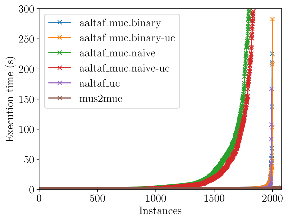
The cactus plot in Figure 1(a) reports the performance of different systems in this task. Overall, we can observe that most of the formulae are trivial for all systems, resulting in sub-second runtimes. Figure 1(b) “zooms-in” to the hardest instances, were we observe that the aaltaf-muc.binary and aaltaf-muc.binary-uc are faster than aaltaf-uc, although the task solved by aaltaf-uc is easier (since it does not provide minimality guarantees on the UC). These results match the experimental results in (Niu et al. 2023). Overall, mus2muc outperforms all systems in this task.
Enumeration of MUCs.
Our second experiment consists in evaluating mus2muc effectiveness in enumerating MUCs of the formulae in the benchmark suite. Table 1 reports statistics about the number of found MUCs, probe depth and size of MUCs (i.e., number of conjuncts).
In general, different formula families exhibit heterogeneous behavior, ranging from easy (e.g., fully enumerated within seconds) to hard — yielding a number of MUCs in the order of thousands per instance, that cannot be fully enumerated within the timeout. In particular, some of the easy families can be fully-enumerated with a probe depth that does not exceed one. Essentially, all inconsistencies can be detected at a propositional level, involving no temporal reasoning.
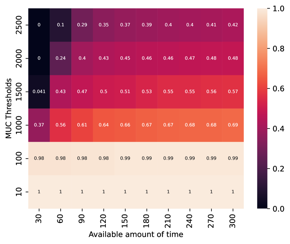
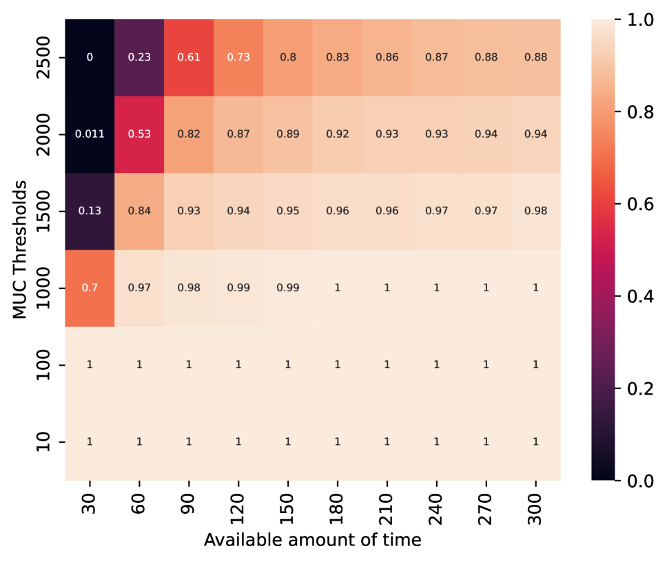
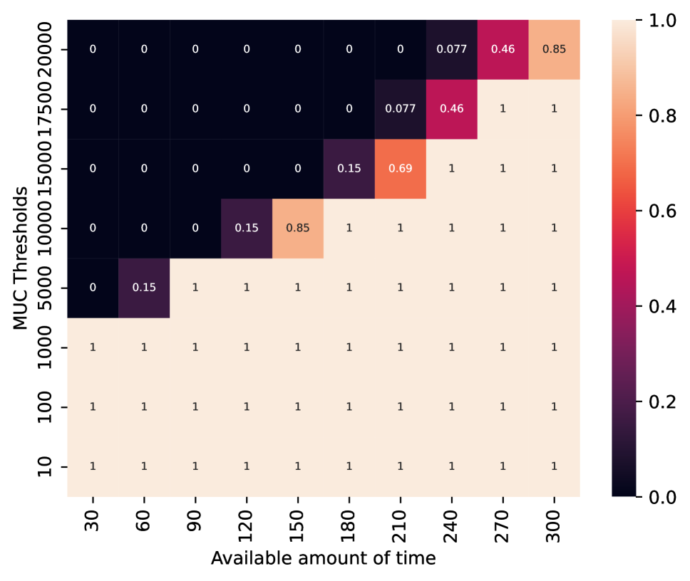
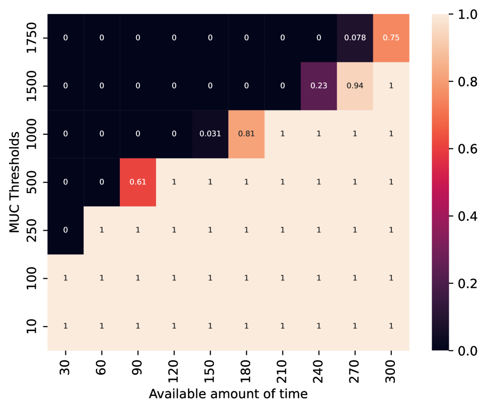
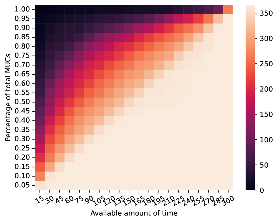
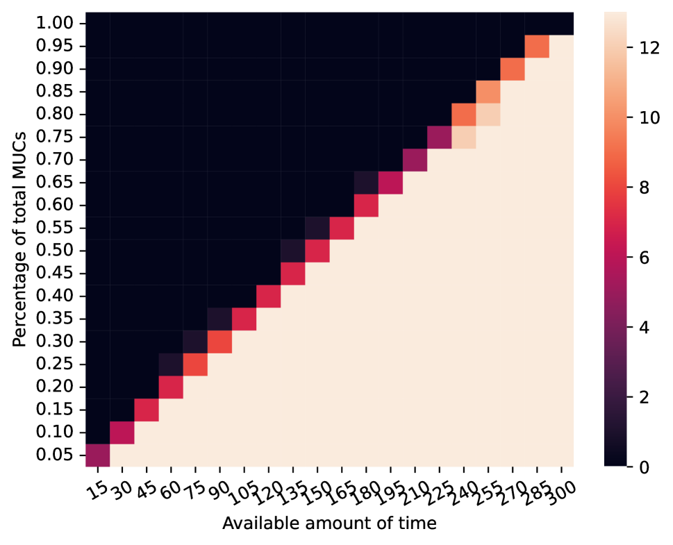
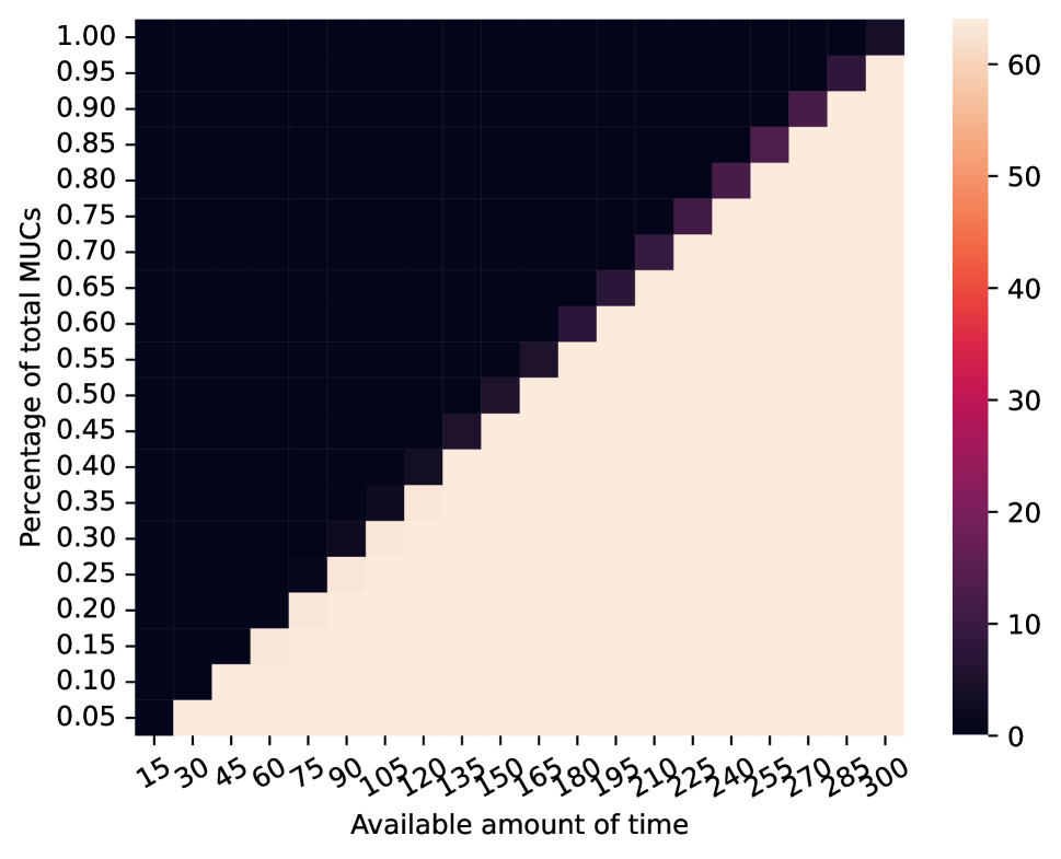
For the remaining formula families, we study how fast MUCs are extracted using mus2muc. The heatmaps in figures 2(a)- 2(d) report, for distinct families, in a cell the percentage of instances for which mus2muc can produce at least MUCs in at most seconds. Even on these formulae, our approach is able to output a considerable amount of MUCs in short time, albeit not able to fully enumerate them within the timeout. Conversely, the heatmaps in figures 3(a)- 3(d) report how MUCs are “temporally distributed” within the timeout. For distinct families, a cell contains the number of instances where it is possible to find percent of found MUCs (i.e., enumerated within timeout) within seconds. We can see that for all these families, in the majority of instances a MUCs are computed in a steady fashion and MUCs become available within seconds of runtime. Instances in these families are characterized by a huge number of MUCs that cannot be realistically inspected. However, even if in this scenario, our approach can provide a reasonable number of MUCs within few seconds.
Generation vs. Certification.
In the mus2muc system, following Algorithm 2, each (unique) MUS extracted from the probe is checked for satisfiability by an LTL solver, to be either certified (e.g., found unsatisfiable) or disproved (e.g., there exists a satisficing trace whose length exceeds the current probe depth). In our implementation, MUS search and MUS certification run concurrently rather than in an interleaved fashion. Given the modularity of our approach, it is interesting to study which component affects runtimes the most. To this end, we consider formula families that are not fully enumerated within timeout, but behave differently from the ones considered in the previous experiment.
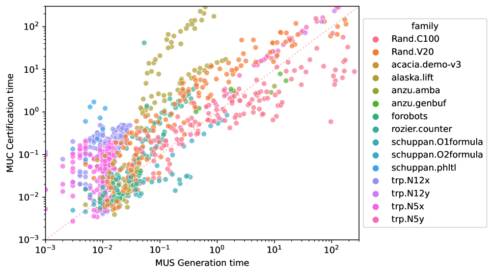
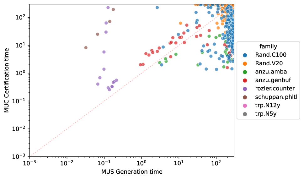
In particular, when performing MUC extraction over an instance , a certain amount of seconds due to MUS generation and MUS certification are accrued. Scatter plots in Figure 4 report each instance as a point , where is the total CPU time spent running MUS generation procedures and is the total CPU time spent running MUS certification888Notice that, for a given instance, MUS generation runtimes and MUS certification runtimes do not necessarily sum up to the timeout since components run concurrently (i.e., CPU time could be greater than wall time). Furthermore, if a timeout signal is received while a MUC is being certified, aaltaf can’t output any timestamp. Same goes for wasp during MUS generation. This explains not-fully-enumerated instances below the upper-right corner of the scatter plot.. Colors denote which family each data-point belongs to.
We can observe in Figure 4(b) that MUS generation and MUC certification can both become bottlenecks in mus2muc, for unsatisfiable instances. Notably, some formula families such as feature unsatisfiable instances for which wasp is able to provide MUSes in less than a second, but whose certification time exceeds the allowed runtime. Similarly, in the random conjunction family features instances for which the cumulative certification time is one order of magnitude smaller than MUS generation time. This sort of trade-off can be better analyzed by considering only fully enumerated instances in Figure 4(a), where it is possible to observe heterogeneous behavior among families, ranging from families that are trivial from both standpoints (lower left corner); hard from both standpoints (upper right corner); easy MUS generation-wise, but hard MUC-certification wise (upper left corner). No fully-enumerated instances are easy certification-wise and hard generation-wise — as we have a mostly empty lower right corner in scatter plot.
Domain-agnostic MUCs enumeration techniques.
As far as we know, no publicly available systems work out of the box to enumerate MUCs of LTL formulae. However, a number of general purpose, domain-agnostic MUC extraction algorithms (which also support LTL as a domain) are available (Bendík and Cerna 2018). The survey by (Roveri et al. 2024), does not compare with algorithms proposed in (Bendík and Cerna 2018).
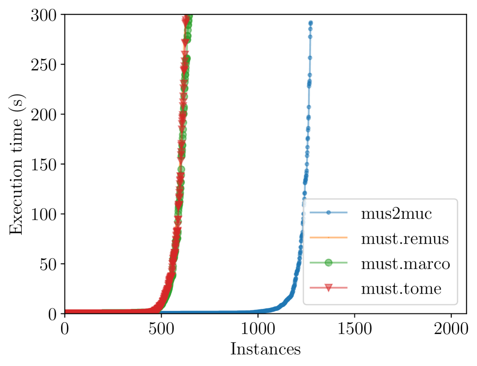
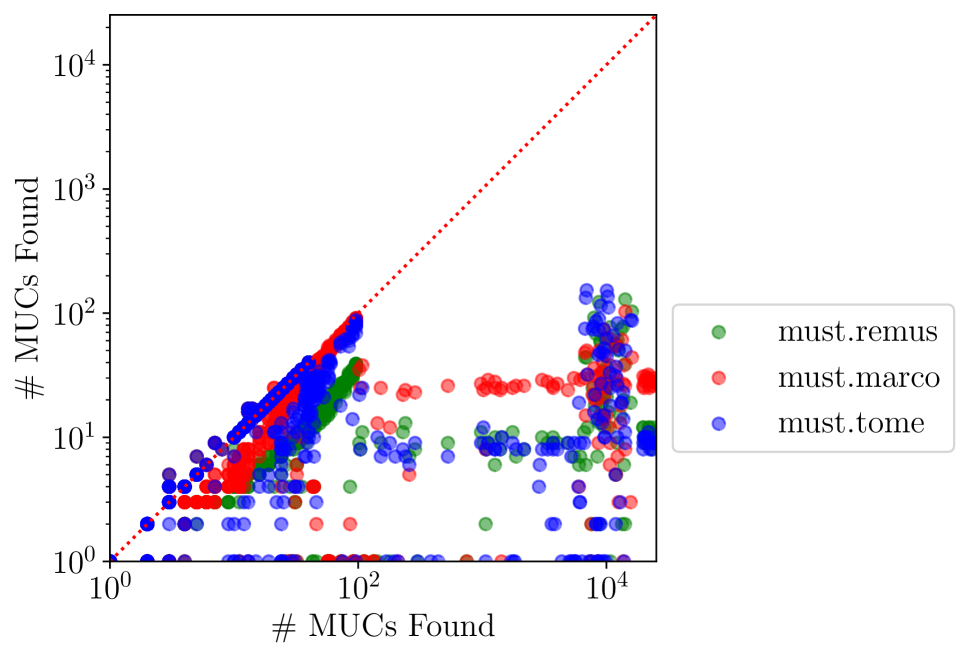
Figure 5(a) compares the number of fully-enumerated instances among different must algorithms and mus2muc. mus2muc is more effective, and can fully-enumerate more or less 500 more instances than any must variant. All must variants perform roughly the same. Figure 5(b) compares the number of found MUCs of each must variant wrt mus2muc. A point in Figure 5(b), denotes that for a given instance in the benchmarks suite mus2muc has computed MUCs whereas one of the must algorithms has computed MUCs. Each color distinguish a specific must algorithm.
We can see, from the cactus plot in Figure 5(a), that different algorithms of must are able to fully-enumerate (roughly) the same number of instances, indeed corresponding lines are mostly overlapped. Overall, mus2muc is able to enumerate more MUCs than any of the must variants — in some extreme cases, enumerating several order of magnitude more MUCs (see the points that lie on the -axis).
Conclusions
Satisfiability of temporal specifications expressed in LTL play an important role in several artificial intelligence application domains (Bacchus and Kabanza 1998; Calvanese, De Giacomo, and Vardi 2002; De Giacomo et al. 2016; De Giacomo and Vardi 1999; De Giacomo et al. 2019). Therefore, in case of unsatisfiable specifications, detecting reasons for unsatisfiability — e.g., computing its minimal unsatisfiable cores — is of particular interest. This is especially true whenever the specification under analysis is expected to be satisfiable.
Recent works (Niu et al. 2023; Roveri et al. 2024) propose several approaches for single MUC computation, but do not investigate enumeration techniques for MUCs.
However, enumerating MUCs for LTL specifications is pivotal to enabling several reasoning services, such as some explainability tasks (Miller 2019), as it is the case for propositional logic (Marques-Silva 2010; Marques-Silva, Janota, and Mencía 2017).
In this paper, we propose an approach for characterizing MUCs of LTL formulae as minimal unsatisfiable subprograms (MUS) of suitable logic programs, introducing the notion of probe. This enables to implement LTL MUC enumeration techniques by exploiting off-the-shelf ASP and LTL reasoners, similarly to SAT-based domain agnostic MUC enumeration techniques à la (Bendík and Cerna 2018).
The approach presented herein is modular with respect to ASP & LTL reasoners, which essentially constitute two sub-modules of the system, and with respect to the logic program that is used to extract MUCs via its MUSes.
We implement this strategy in mus2muc, using the ASP solver wasp and the LTL solver aaltaf. Our experiments show mus2muc is effective at enumerating MUCs of unsatisfiable formulae that are commonly used in LTL literature as benchmarks, as well as being competitive with available state-of-the-art for single MUC computation.
To the best of our knowledge, this represent the first attempt to address this task in the LTL setting.
As far as future works are concerned, we are interested in studying how the choice of probes affect MUCs computation in our setting, as well as providing ad-hoc implementations for closely related LTL tasks, such explaining and repairing incosistent Declare specification in the realm of process mining.
References
- Alviano et al. (2023) Alviano, M.; Dodaro, C.; Fiorentino, S.; Previti, A.; and Ricca, F. 2023. ASP and subset minimality: Enumeration, cautious reasoning and MUSes. Artif. Intell., 320: 103931.
- Audemard, Koriche, and Marquis (2020) Audemard, G.; Koriche, F.; and Marquis, P. 2020. On Tractable XAI Queries based on Compiled Representations. In KR, 838–849.
- Baader and Peñaloza (2010) Baader, F.; and Peñaloza, R. 2010. Automata-Based Axiom Pinpointing. J. Autom. Reason., 45(2): 91–129.
- Bacchus and Kabanza (1998) Bacchus, F.; and Kabanza, F. 1998. Planning for Temporally Extended Goals. Ann. Math. Artif. Intell., 22(1-2): 5–27.
- Bendík and Cerna (2018) Bendík, J.; and Cerna, I. 2018. Evaluation of Domain Agnostic Approaches for Enumeration of Minimal Unsatisfiable Subsets. In LPAR, volume 57 of EPiC Series in Computing, 131–142. EasyChair.
- Brewka, Eiter, and Truszczynski (2011) Brewka, G.; Eiter, T.; and Truszczynski, M. 2011. Answer set programming at a glance. Commun. ACM, 54(12): 92–103.
- Brewka, Thimm, and Ulbricht (2019) Brewka, G.; Thimm, M.; and Ulbricht, M. 2019. Strong inconsistency. Artif. Intell., 267: 78–117.
- Calimeri et al. (2020) Calimeri, F.; Faber, W.; Gebser, M.; Ianni, G.; Kaminski, R.; Krennwallner, T.; Leone, N.; Maratea, M.; Ricca, F.; and Schaub, T. 2020. ASP-Core-2 Input Language Format. Theory Pract. Log. Program., 20(2): 294–309.
- Calvanese, De Giacomo, and Vardi (2002) Calvanese, D.; De Giacomo, G.; and Vardi, M. Y. 2002. Reasoning about Actions and Planning in LTL Action Theories. In KR, 593–602.
- Chiariello et al. (2024) Chiariello, F.; Fionda, V.; Ielo, A.; and Ricca, F. 2024. A Direct ASP Encoding for Declare. In PADL, volume 14512 of Lecture Notes in Computer Science, 116–133. Springer.
- De Giacomo et al. (2019) De Giacomo, G.; Iocchi, L.; Favorito, M.; and Patrizi, F. 2019. Foundations for Restraining Bolts: Reinforcement Learning with LTLf/LDLf Restraining Specifications. In ICAPS, 128–136. AAAI Press.
- De Giacomo et al. (2016) De Giacomo, G.; Maggi, F. M.; Marrella, A.; and Sardiña, S. 2016. Computing Trace Alignment against Declarative Process Models through Planning. In ICAPS, 367–375.
- De Giacomo and Vardi (1999) De Giacomo, G.; and Vardi, M. Y. 1999. Automata-Theoretic Approach to Planning for Temporally Extended Goals. In ECP, volume 1809 of LNCS, 226–238.
- De Giacomo and Vardi (2013) De Giacomo, G.; and Vardi, M. Y. 2013. Linear Temporal Logic and Linear Dynamic Logic on Finite Traces. In IJCAI, 854–860. IJCAI/AAAI.
- Di Ciccio and Montali (2022) Di Ciccio, C.; and Montali, M. 2022. Declarative Process Specifications: Reasoning, Discovery, Monitoring. In van der Aalst, W. M. P.; and Carmona, J., eds., Process Mining Handbook, volume 448 of Lecture Notes in Business Information Processing, 108–152. Springer.
- Fionda and Greco (2018) Fionda, V.; and Greco, G. 2018. LTL on Finite and Process Traces: Complexity Results and a Practical Reasoner. J. Artif. Intell. Res., 63: 557–623.
- Fionda, Ielo, and Ricca (2024) Fionda, V.; Ielo, A.; and Ricca, F. 2024. ltlf2asp: LTLf Bounded Satisfiability in ASP. In LPNMR, volume (to appear) of Lecture Notes in Computer Science, 0–0. Springer.
- Geatti et al. (2024) Geatti, L.; Gigante, N.; Montanari, A.; and Venturato, G. 2024. SAT Meets Tableaux for Linear Temporal Logic Satisfiability. J. Autom. Reason., 68(2): 6.
- Gebser et al. (2019) Gebser, M.; Kaminski, R.; Kaufmann, B.; and Schaub, T. 2019. Multi-shot ASP solving with clingo. Theory Pract. Log. Program., 19(1): 27–82.
- Gelfond and Lifschitz (1991) Gelfond, M.; and Lifschitz, V. 1991. Classical Negation in Logic Programs and Disjunctive Databases. New Gener. Comput., 9(3/4): 365–386.
- Li et al. (2020a) Li, J.; Pu, G.; Zhang, Y.; Vardi, M. Y.; and Rozier, K. Y. 2020a. SAT-based explicit LTLf satisfiability checking. Artif. Intell., 289: 103369.
- Li et al. (2020b) Li, J.; Pu, G.; Zhang, Y.; Vardi, M. Y.; and Rozier, K. Y. 2020b. SAT-based explicit LTLf satisfiability checking. Artif. Intell., 289: 103369.
- Liffiton et al. (2016) Liffiton, M. H.; Previti, A.; Malik, A.; and Marques-Silva, J. 2016. Fast, flexible MUS enumeration. Constraints An Int. J., 21(2): 223–250.
- Liffiton and Sakallah (2008) Liffiton, M. H.; and Sakallah, K. A. 2008. Algorithms for Computing Minimal Unsatisfiable Subsets of Constraints. J. Autom. Reason., 40(1): 1–33.
- Maggi, Montali, and Peñaloza (2020) Maggi, F. M.; Montali, M.; and Peñaloza, R. 2020. Temporal Logics Over Finite Traces with Uncertainty. In The Thirty-Fourth AAAI Conference on Artificial Intelligence, AAAI 2020, 10218–10225. AAAI Press.
- Marques-Silva (2010) Marques-Silva, J. 2010. Minimal Unsatisfiability: Models, Algorithms and Applications (Invited Paper). In ISMVL, 9–14. IEEE Computer Society.
- Marques-Silva, Janota, and Mencía (2017) Marques-Silva, J.; Janota, M.; and Mencía, C. 2017. Minimal sets on propositional formulae. Problems and reductions. Artif. Intell., 252: 22–50.
- Meliou, Roy, and Suciu (2014) Meliou, A.; Roy, S.; and Suciu, D. 2014. Causality and Explanations in Databases. Proc. VLDB Endow., 7(13): 1715–1716.
- Mencía and Marques-Silva (2014) Mencía, C.; and Marques-Silva, J. 2014. Efficient Relaxations of Over-constrained CSPs. In Proceedings of 26th IEEE International Conference on Tools with Artificial Intelligence, ICTAI 2014, 725–732. IEEE Computer Society.
- Mencía and Marques-Silva (2020) Mencía, C.; and Marques-Silva, J. 2020. Reasoning About Strong Inconsistency in ASP. In SAT, volume 12178 of Lecture Notes in Computer Science, 332–342. Springer.
- Miller (2019) Miller, T. 2019. Explanation in artificial intelligence: Insights from the social sciences. Artif. Intell., 267: 1–38.
- Morgado et al. (2013) Morgado, A.; Heras, F.; Liffiton, M. H.; Planes, J.; and Marques-Silva, J. 2013. Iterative and core-guided MaxSAT solving: A survey and assessment. Constraints An Int. J., 18(4): 478–534.
- Niu et al. (2023) Niu, T.; Xiao, S.; Zhang, X.; Li, J.; Huang, Y.; and Shi, J. 2023. Computing minimal unsatisfiable core for LTL over finite traces. Journal of Logic and Computation, exad049.
- Peñaloza (2019) Peñaloza, R. 2019. Explaining Axiom Pinpointing. In Lutz, C.; Sattler, U.; Tinelli, C.; Turhan, A.; and Wolter, F., eds., Description Logic, Theory Combination, and All That - Essays Dedicated to Franz Baader on the Occasion of His 60th Birthday, volume 11560 of Lecture Notes in Computer Science, 475–496. Springer.
- Peñaloza (2020) Peñaloza, R. 2020. Axiom Pinpointing. In Cota, G.; Daquino, M.; and Pozzato, G. L., eds., Applications and Practices in Ontology Design, Extraction, and Reasoning, volume 49 of Studies on the Semantic Web, 162–177. IOS Press.
- Peñaloza and Ricca (2022) Peñaloza, R.; and Ricca, F. 2022. Pinpointing Axioms in Ontologies via ASP. In Gottlob, G.; Inclezan, D.; and Maratea, M., eds., Proceedings of LPNMR 2022, volume 13416 of Lecture Notes in Computer Science, 315–321. Springer.
- Pesic, Schonenberg, and van der Aalst (2007) Pesic, M.; Schonenberg, H.; and van der Aalst, W. M. P. 2007. DECLARE: Full Support for Loosely-Structured Processes. In Proceedings of EDOC 2007, 287–300. IEEE Computer Society.
- Pnueli (1977) Pnueli, A. 1977. The Temporal Logic of Programs. In FOCS, 46–57. IEEE Computer Society.
- Reynolds (2016) Reynolds, M. 2016. A New Rule for LTL Tableaux. In GandALF, volume 226 of EPTCS, 287–301.
- Roveri et al. (2024) Roveri, M.; Ciccio, C. D.; Francescomarino, C. D.; and Ghidini, C. 2024. Computing Unsatisfiable Cores for LTLf Specifications. J. Artif. Intell. Res., 80: 517–558.
- Schlobach and Cornet (2003) Schlobach, S.; and Cornet, R. 2003. Non-Standard Reasoning Services for the Debugging of Description Logic Terminologies. In Gottlob, G.; and Walsh, T., eds., Proceedings of IJCAI’03, 355–362. Morgan Kaufmann.
- Schuppan and Darmawan (2011) Schuppan, V.; and Darmawan, L. 2011. Evaluating LTL Satisfiability Solvers. In ATVA, volume 6996 of Lecture Notes in Computer Science, 397–413. Springer.
- Sebastiani and Vescovi (2009) Sebastiani, R.; and Vescovi, M. 2009. Axiom Pinpointing in Lightweight Description Logics via Horn-SAT Encoding and Conflict Analysis. In Schmidt, R. A., ed., Procedding of the 22nd International Conference on Automated Deduction, volume 5663 of Lecture Notes in Computer Science, 84–99. Springer.