MAC-VO: Metrics-aware Covariance for Learning-based
Stereo Visual Odometry
mac-vo.github.io

Abstract

We propose the MAC-VO, a novel learning-based stereo VO that leverages the learned metrics-aware matching uncertainty for dual purposes: selecting keypoint and weighing the residual in pose graph optimization. Compared to traditional geometric methods prioritizing texture-affluent features like edges, our keypoint selector employs the learned uncertainty to filter out the low-quality features based on global inconsistency. In contrast to the learning-based algorithms that model the scale-agnostic diagonal weight matrix for covariance, we design a metrics-aware covariance model to capture the spatial error during keypoint registration and the correlations between different axes. Integrating this covariance model into pose graph optimization enhances the robustness and reliability of pose estimation, particularly in challenging environments with varying illumination, feature density, and motion patterns. On public benchmark datasets, MAC-VO outperforms existing VO algorithms and even some SLAM algorithms in challenging environments. The covariance map also provides valuable information about the reliability of the estimated poses, which can benefit decision-making for autonomous systems.

I Introduction

Visual Odometry (VO) predicts the relative camera pose from image sequences and often serves as the front-end of Simultaneous Localization and Mapping (SLAM) systems. Over the past few decades, both geometric and learning-based methods have been developed with significant advances in generalizability and accuracy [1, 2, 3, 4]. However, VO remains a challenging problem in real-world scenarios, with multiple visual degraded scenarios such as low illumination, dynamic and texture-less scenes.

To improve the robustness in challenging scenes, geometric-based VO algorithms employ outlier filtering strategies [5] and weigh the optimization residuals by the covariance of the observed features [6]. However, how to effectively select the reliable keypoints and model their covariance becomes two significant challenges. Existing methods typically select the keypoints based on local intensity gradient with a manually defined threshold [7, 8, 9]. These approaches leads to errors and outliers because it doesn’t model the structure or context information of the environment (e.g. features on repetitive patterns may not be ideal candidates despite high image gradients). Moreover, the covariance model is often empirically modeled using a constant parameter, which is sub-optimal. In addition, the parameters in keypoint selection and covariance model need to be extensively tuned for different environments.

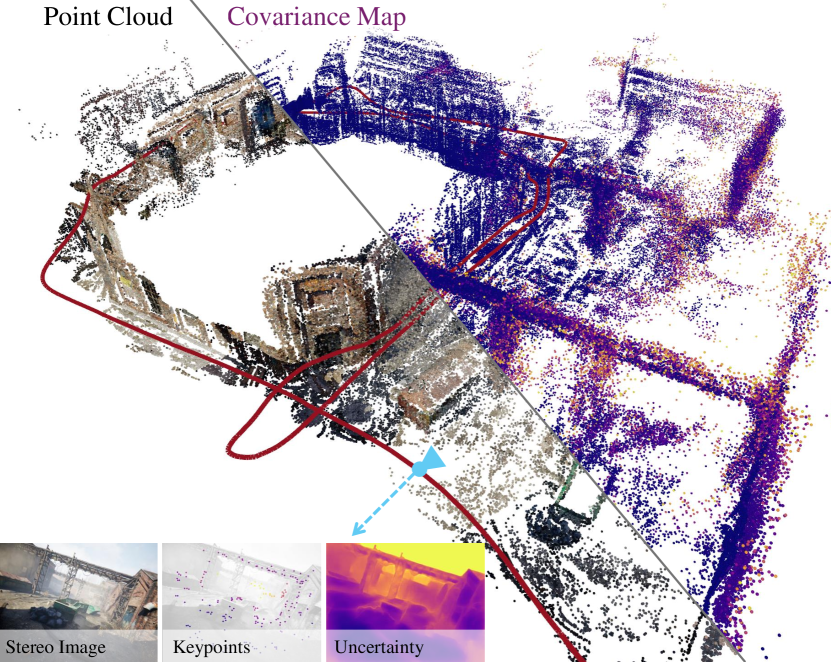
Figure 1: Without relying on multi-frame bundle adjustment, MAC-VO aggregately reconstruct the map based on the two-frame Pose graph optimization. We propose metrics-aware covariance model for 3D keypoint based on the learning matching uncertainty. The covariance model serves dual purposes: selecting keypoints and weighing the residual in the pose graph optimization.

With advances in learning-based visual features, more algorithms utilize learned features [7] to optimize the camera pose. Confidence score [10] or confidence weights [3, 4] of these feature points are often obtained in an unsupervised manner. The learned confidence helps to track the features and model the reliability during the optimization. However, these confidence or uncertainty values are scale-agnostic, which means they don’t reflect the actual estimation error in the 3D space. This scale-agnostic problem brings two limitations. Firstly, it makes the covariance inconsistent across different environments that vary in scale, such as indoors and outdoors. Secondly, it makes it harder to integrate multiple constraints from different modalities or sensors.

To overcome the above challenges, this paper addresses the problem of modeling metrics-aware covariance values for the 3D keypoints. More specifically, this is achieved through two innovations. Firstly, we propose a learning-based model to quantify the 2D metrics-aware uncertainty of feature matching. Inspired by the FlowFormer [11] and GMA [12], we employ an iterative update model and motion aggregator to predict the uncertainty in 2D image space, which helps to filter unreliable features in the occluded region or low-illumination area. Secondly, based on the learned 2D uncertainty values, we model the covariance of the feature points in 3D space using a metrics-aware 3D covariance model. Compared to DROID-SLAM [3], which utilizes a scale-agnostic diagonal covariance matrix, our approach provides a more accurate representation by modeling the covariance of 3D feature points. This covariance model includes the inter-axes correlation of the 3D features. In the ablation study, we demonstrate the inter-frame consistency and the intra-frame consistency of our proposed covariance model.

We integrate the above two innovations into MAC-VO, a stereo VO that features superior keypoint selection and pose graph optimization based on the metrics-aware covariance model and achieves accurate tracking results in challenging cases compared with state-of-the-art VOs and even some SLAM systems without fine-tuning and without multi-frame optimization. In summary, the main contributions are:

• We present a learning-based 2D uncertainty network with metrics awareness, leveraging iterative motion aggregator to capture the inconsistency of the feature matching. This metrics-aware uncertainty evaluates the quality of features in the keypoint selector and weights the residual of backend optimization.

• This paper introduces a novel metrics-aware 3D covariance model based on the 2D uncertainty of feature matching and depth estimation. The ablation study demonstrates the necessity of scale consistency and the off-diagonal terms in the pose graph optimization.

• We propose the MAC-VO, a stereo VO pipeline that estimates the camera pose and registers 3D features with metrics-aware covariance. In the experiments, MAC-VO outperforms existing VO algorithms even some SLAM algorithms in challenging environments.

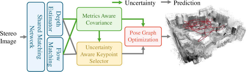
Figure 2: MAC-VO pipeline. We use a shared matching network to estimate the depth, flow, and corresponding uncertainty. The learned uncertainty is leveraged to filter out unreliable features and model the metrics-aware covariance of the 3D keypoints. These registered keypoints and their covariance models are then utilized in the back-end optimization to determine the relative camera pose.

II Related Works

Existing geometric-based methods optimize the camera pose based on geometric constraints like re-projection error [1, 13] or photometric error [14, 15, 16]. To more accurately model the uncertainty of the depth, Civera et al. [17] and Montiel[18] investigate the inverse depth parameterization. These methods often use constant parameters and simple heuristics to model the covariance matrix of these errors during the factor graph optimization. For multi-sensor fusion [6, 19] and semantic SLAM [20, 21], the covariance model plays a significant role in weighing the confidence of different sensors and modules. To effectively capture sensor uncertainty, the covariance models are often tuned based on empirical prior. However, these simplified covariance models fail to capture the complexity of the challenging environments.

Recent advances in deep learning have transformed research in optical flow estimation [22, 23], feature matching [24, 10], depth estimation [25, 26, 27], and end-to-end camera pose estimation [28, 2]. Several methodologies have been developed to address the uncertainty in estimating depth, flow, and pose. Dexheimer et al. [29] proposed a learned depth covariance function that is applied in downstream tasks like 3D reconstruction. Nie et al. utilize a self-supervised learning method to jointly train depth and depth covariance of images in the wild [30]. ProbFlow [31] proposes using post-hoc confidence measures to assess the per-pixel reliability of flow.

Amidst these developments, hybrid learning-based SLAM systems [32, 26, 33, 34, 35, 36] are emerging to synergize the geometric constraint with the adaptability of learning-based methods. To improve the reliability of the feature tracking process, some methods introduce learning-based uncertainty measurements or confidence scores [37, 38, 10] for pose optimization. DROID-SLAM [3] utilizes a differentiable bundle adjustment layer to implicitly tune the uncertainty model. This method employs a simplified diagonal covariance model for the bundle adjustment. These methods focus on the relative confidence between features , but ignore the scale consistency of the covariance model.

For keypoint selection, geometric-based VO relies on hand-crafted features [8, 9], which detect the edges and corner points. The recent advance of the learning-based method train feature extractor in data-driven manner [7, 39]. However, these keypoint also prioritize the edge and corner features due to their data bias in the pre-training dataset. Recent works like D3VO [32] have shown that relying on edge and corner points can degrade state estimation, sometimes performing worse than random selectors [4]. The accuracy of learning-based feature matching and depth estimation algorithms is particularly compromised at object edges due to feature interpolation and the ambiguity in neural networks. In this work, we propose a keypoint selector based on learned uncertainty to filter out the unreliable features.

III Method

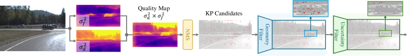
Figure 3: We include three filters: Non-minimum Suppression (NMS) filter, geometric filter, and uncertainty-based filter. In the KITTI dataset, the uncertainty filter implicitly filters out the unreliable feature matchings in the scene.

As illustrated in Figure 2, MAC-VO outlines an effective integration of a learning-based front-end and a geometrically constrained back-end using the metrics-aware covariance model. In the front-end (Section III-A), we train an uncertainty-aware matching network to model the corresponding uncertainty stems from feature deficiencies. Utilizing the learned uncertainty, we develop a keypoint selector in Section III-B to choose reliable features. The metrics-aware 2D uncertainty is then propagated to the 3D space via the proposed covariance model in Section. III-C. In the back-end optimization (Section. III-D), we optimize the relative motion by minimizing the distance between registered keypoints weighted by the 3D covariance.

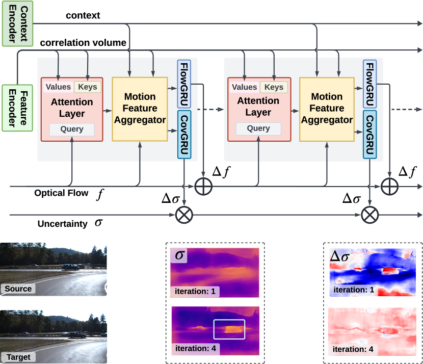
Figure 4: Top: Architecture of the uncertainty-aware matching network. We employ a motion aggregator and an iterative update structure to enable the covariance module to capture inconsistencies in feature matching. Bottom: In each iteration, the model captures the inconsistency between the motions. For the $\Delta\sigma$, the red color indicates a positive $\Delta\sigma$ that increases the uncertainty, and blue means decreasing the uncertainty.

III-A Network & Uncertainty Training

The objective of our network is to predict the flow $\hat{f}\in\mathbb{R}^{2}$ and the corresponding uncertainty $\hat{\Sigma}_{f}=\mathrm{diag}(\sigma_{u}^{2},\sigma_{v}^{2})$. As shown in Fig. 4, an iterative motion aggregator inspired by the FlowFormer [11] is employed to capture the inconsistency in feature matching. To extend this network for uncertainty estimation, we add an uncertainty decoder to predict the $\Delta\sigma$ updates of the uncertainty in the log space. The use of log space enables additive updates and constrains the output range, stabilizing gradients and simplifying model output. After iterative updates, the log-variance passes through an exp activation function to obtain the final uncertainty. More details about the network are shown in Appendix. B-E.

To supervise the uncertainty, we leverage the negative log-likelihood loss used in conformal prediction [40, 41, 42]:

$$\mathcal{L}_{cov}=\sum_{i}^{N}\alpha_{i}\left((y-f_{i})^{\top}\hat{\Sigma}_{f}^{-1}(y-f_{i})+\log(\det\hat{\Sigma}_{f})\right),$$ (1)

where $y$ is the ground truth optical flow, $f_{i}$ denotes the $i$-th iteration of the network outputs, and $\alpha_{i}$ is the weight for each iteration and is set to decrease exponentially with ratio of $0.8$. During the training stage, we initialize the encoder network parameters with the pre-trained model by FlowFormer. We then train the covariance module on the synthetic dataset TartanAir [43]. Our experiments demonstrate that the model can generalize to real-world datasets without fine-tuning.

III-B Uncertainty-based Keypoint Selection

Different from the random selector used in DPVO[4] and the hand-crafted features used in ORB-SLAM [8], we leverage the learned uncertainty estimation to filter out unreliable features such as those on the vehicle illustrated in Fig. 3. This is achieved by composing three filters: the uncertainty filter, geometry filter, and the non-minimum suppression (NMS). The uncertainty filter removes pixels with depth and flow uncertainty larger than $1.5$ times the median uncertainty of the current frame, which discards the unreliable features while maintaining the diversity of keypoint candidates. The accurate uncertainty estimation effectively removes the keypoints on occluded objects, reflective surfaces, and feature-less areas. Illustrated in Fig. 3, the uncertainty filter removes all keypoint candidates on the moving vehicle on a KITTI trajectory due to its high flow uncertainty. Along with the uncertainty filter is the geometric filter, which constraints the disparity and removes keypoints on the edge of frame. To ensure the even distribution of keypoints in image, the NMS filter is applied on the product of depth and flow uncertainty map prior to both filters.

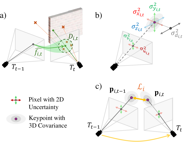
Figure 5: a) Uncertain estimation of depth due to the error in feature matching. b) Projecting depth and matching uncertainty from image plane to 3D space. c) Residual $\mathcal{L}_{i}$ for pose graph optimization.

III-C Metrics-aware 3D Covariance Model

In the context of the camera projection geometry, the covariance of a 3D keypoint is determined by the uncertainty of the depth $\sigma_{d}^{2}$ and matching $(\sigma_{u}^{2},\sigma_{v}^{2})$. To accurately model the covariance for 3D keypoint, it is critical to determine (1) the depth uncertainty of the matched points $\hat{\sigma}_{d}^{2}$ and (2) the off-diagonal covariance terms during the 2D-3D projection process.

Depth Uncertainty after keypoint matching  As shown in Fig. 5 (a), the matched features are expected to be within a probabilistic range centered at $[u_{i,t},v_{i,t}]$ due to flow uncertainty $(\sigma_{u_{i,t}}^{2},\sigma_{v_{i,t}}^{2})$. As a result, a minor disturbance in the feature matching may introduce a large error in the depth.

To address this problem, we model the depth uncertainty $\hat{\sigma}_{d_{i,t}}^{2}$ of the matched feature point based on the depth feature of the local patch $D_{i,t}$. We approximate it with the weighted sum of the variances within the patch. The weights are determined by a 2D Gaussian kernel $\varphi$, which utilizes $\sigma_{u_{i,t}}^{2}$ and $\sigma_{v_{i,t}}^{2}$ to adjust the influence of each point within the patch: $\sigma_{d_{i,t}}^{2}=\sum_{j}{\varphi_{j}(d_{j}-\mu_{{D}_{i,t}})^{2}}.$

Project 2D Uncertainty to 3D Covariance  Following the pinhole camera model with focus $\mathrm{f}_{x},\mathrm{f}_{y}$ and optical center $\mathrm{c}_{x},\mathrm{c}_{y}$, the coordinate of the keypoint is calculated by: $\mathbf{x}_{i,t}=(\mathbf{u}_{i,t}-\mathrm{c}_{x})\mathbf{d}_{i,t}/\mathrm{f}_{x}$, $\mathbf{y}_{i,t}=(\mathbf{v}_{i,t}-\mathrm{c}_{y})\mathbf{d}_{i,t}/\mathrm{f}_{y}$ and $\mathbf{z}_{i,t}=\mathbf{d}_{i,t}$, as shown in Fig. 5 (b). To accurately capture the uncertainties associated with these measurements, the main diagonal of the covariance matrix is formulated as:

$$\sigma_{x_{i,t}}^{2} ={((\sigma_{u_{i,t}}^{2}+d^{2}_{i,t})(\sigma_{d_{i,t}}^{2}+u^{2}_{i,t})-u^{2}_{i,t}d^{2}_{i,t}+\mathrm{c}_{x}^{2}\sigma_{d_{i,t}}^{2})}/{\mathrm{f}_{x}^{2}},$$ (2)

$$\sigma_{y_{i,t}}^{2} ={((\sigma_{v_{i,t}}^{2}+d_{i,t}^{2})(\sigma_{d_{i,t}}^{2}+v_{i,t}^{2})-v_{i,t}^{2}d_{i,t}^{2}+\mathrm{c}_{y}^{2}\sigma_{d_{i,t}}^{2})}/{\mathrm{f}_{y}^{2}},$$

$$\quad\sigma_{z_{i,t}}^{2} =\sigma_{d_{i,t}}^{2}.$$

In this model, the projected coordinates are interdependent due to the common multiplier of depth $\mathbf{d}_{i,t}$. To precisely formulate the covariance of the 3D keypoints ${}^{c}\Sigma_{i,t}^{p}$ under camera coordinate, it is essential to include the off-diagonal covariance terms in ${}^{c}\Sigma_{i,t}^{p}$.

$${}^{c}\Sigma_{i,t}^{p}=\begin{bmatrix}\sigma_{z}^{2}&\sigma_{xz_{i,t}}&\sigma_{yz_{i,t}}\\ \sigma_{xz_{i,t}}&\sigma_{x_{i,t}}^{2}&\sigma_{xy_{i,t}}\\ \sigma_{yz_{i,t}}&\sigma_{xy_{i,t}}&\sigma_{y_{i,t}}^{2}\\ \end{bmatrix},\;\begin{aligned} &\sigma_{xz}=\sigma_{d}^{2}(u-\mathrm{c}_{x})/\mathrm{f}_{x}\\ &\sigma_{yz}=\sigma_{d}^{2}(v-\mathrm{c}_{y})/\mathrm{f}_{y}\\ &\sigma_{xy}=\frac{\sigma_{d}^{2}(u-\mathrm{c}_{x})(v-\mathrm{c}_{y})}{\mathrm{f}_{x}\mathrm{f}_{y}}.\end{aligned}$$ (3)

Results in the ablation study also confirm the necessity of off-diagonal terms for accurate pose graph optimization. Detailed derivation for Eq. 2 and Eq. 3 is in Appendix. A-C.

III-D Pose Graph Optimization

We optimize the camera pose $T_{t}\in SE(3)$ at time $t$ in the world frame by minimizing the distance of the matched 3D keypoints $p_{i,t-1}$ and ${}^{c}p_{i,t}$, where ${}^{c}p_{i,t}$ is in the camera frame. To reduce the initial error margin of the optimization, we initialize the camera pose using the relative motion estimated by the TartanVO [2].

The pose graph optimization is formulated as follows:

$$T^{\star} =\operatorname*{arg\,min}_{T_{t}}{\sum_{i}{\left\|p_{i,t-1}-{T}_{t}\,{}^{c}p_{i,t}\right\|^{2}_{\Sigma_{i}}}},$$ (4)

$$\Sigma_{i} =\Sigma_{i,t-1}^{p}+R_{t}\;{}^{c}\Sigma_{i,t}^{p}\;R_{t}^{\top}.$$

$\|\cdot\|_{\Sigma_{i}}$ represents the Mahalanobis distance with covariance matrix $\Sigma_{i}$. Unlike DROID-SLAM [3], which employs a diagonal covariance matrix, we model the correlation between axes to capture accurate inter-dependencies. We solved this optimization problem by Levenberg-Marquardt algorithms using PyPose [44].

IV Experiment

Datasets & Baseline  We evaluate the proposed model and baseline methods on a variety of public datasets, including synthetic dataset TartanAir v2 [43], real-world data from EuRoC [45], KITTI [46], as well as customized data collected from a Zed camera. These datasets cover a diverse range of hardware configurations, motion patterns, and environments. To demonstrate our method’s robustness under challenging scenarios, we collected the TartanAir v2, a new set of difficult trajectories following the TartanAir [43] that includes frequent indoor-outdoor transition and low-illumination scenes as shown in Fig. 6. To demonstrate the generalizability of our model, we use the same configuration across all datasets.

Evaluation Metrics  Our evaluation focuses more on relative error Since the proposed method does not contain loop closure or global bundle adjustment. So we use Relative translation error ($t_{\mathrm{rel}}$, $\mathrm{m/frame}$) and relative rotation error ($r_{\mathrm{rel}}$, $\mathrm{{}^{\circ}/frame}$) as:

$$t_{\mathrm{rel}} =\frac{1}{N}\sum^{N}_{t=1}{\left\|p_{t+1}-p_{t}-R_{t}\hat{R}_{t}^{\top}\!\!\left(\hat{p}_{t+1}-\hat{p_{t}}\right)\right\|_{2}},$$ (5)

$$r_{\mathrm{rel}} =\frac{180}{\pi}\frac{1}{N}\sum^{N}_{t=1}\left\|\log\left(\hat{R}_{t,t+1}^{\top}R_{t,t+1}\right)\right\|_{2},$$

where $p_{t}$ and $R_{t}$ are ground truth position and rotation, $\hat{p}_{t}$ and $\hat{R}_{t}$ is the estimated position and rotation. $R_{t,t+1}=R_{t}^{\top}R_{t+1}$ is the rotation from frame $t$ to frame $t+1$.

IV-A Quantitative Analysis

TABLE I: Performance comparison of different methods on the EuRoC Dataset. Only odd-ordered trajectory is shown due to page limit, see Appendix. B-A for the remaining results.

Trajectory	MH01		MH03		MH05		V102		V201		V203		Avg.‡
	$t_{\mathrm{rel}}$	$r_{\mathrm{rel}}$	$t_{\mathrm{rel}}$	$r_{\mathrm{rel}}$	$t_{\mathrm{rel}}$	$r_{\mathrm{rel}}$	$t_{\mathrm{rel}}$	$r_{\mathrm{rel}}$	$t_{\mathrm{rel}}$	$r_{\mathrm{rel}}$	$t_{\mathrm{rel}}$	$r_{\mathrm{rel}}$	$t_{\mathrm{rel}}$	$r_{\mathrm{rel}}$
SLAM
ORB-SLAM 3	0.0035	0.0450	0.0058	0.0603	0.0059	0.0526	0.0096	0.1757	0.0064	0.1615	0.033	0.9497	0.0092	0.1866
DROID-SLAM⋆	0.0012	0.0159	0.0034	0.2656	0.0025	0.0193	0.0026	0.0417	0.0012	0.0289	0.0034	0.1033	0.0024	0.0590
VO
TartanVO⋆†	0.0121	0.0560	0.0302	0.2791	0.0193	0.0604	0.0251	0.1244	0.0065	0.0920	0.0303	0.2986	0.0198	0.1270
TartanVO	0.0277	0.5122	0.0514	0.6635	0.0464	0.4797	0.0394	1.0420	0.0195	0.4684	0.0473	1.9657	0.0368	0.8346
iSLAM-VO	0.0042	0.0560	0.0076	0.2789	0.0070	0.0603	0.0066	0.1241	0.004	0.0920	0.0151	0.2984	0.0071	0.1269
DPVO⋆†	0.0015	0.0207	0.0028	0.0273	0.0028	0.0243	0.0041	0.0496	0.0016	0.0342	0.0045	0.1205	0.0027	0.0437
Ours	0.0014	0.0214	0.0023	0.0238	0.0025	0.0216	0.0029	0.0434	0.0012	0.0289	0.0049	0.1284	0.0024	0.0403
‡ Average over all trajectories of EuRoC.  † Monocular method.  ⋆ Scale-aligned with ground truth.

EuRoC Dataset    We assessed our model on the EuRoC [45] dataset, as detailed in Table. I, comparing it against baseline methods including visual odometries and state-of-the-art visual SLAM systems with loop-closure and global bundle adjustment. While our method exhibits compatible performance to DROID-SLAM on average $t_{\mathrm{rel}}$, it outperforms all baselines in terms of $r_{\mathrm{rel}}$ by around $10\%$.

TABLE II: Performance comparison on the TartanAir v2 Hard Dataset. Noticeably, ORB-SLAM3 lost track of all sequences and is therefore not included. Only the hard subset is shown due to page limit, see Appendix. VI for the remaining results.

Trajectory	H00		H01		H02		H03		H04		H05		H06		Avg.
	$t_{\mathrm{rel}}$	$r_{\mathrm{rel}}$	$t_{\mathrm{rel}}$	$r_{\mathrm{rel}}$	$t_{\mathrm{rel}}$	$r_{\mathrm{rel}}$	$t_{\mathrm{rel}}$	$r_{\mathrm{rel}}$	$t_{\mathrm{rel}}$	$r_{\mathrm{rel}}$	$t_{\mathrm{rel}}$	$r_{\mathrm{rel}}$	$t_{\mathrm{rel}}$	$r_{\mathrm{rel}}$	$t_{\mathrm{rel}}$	$r_{\mathrm{rel}}$
SLAM
DROID-SLAM⋆	.0485	.1174	.0023	.0210	.0190	.0821	.0064	.0300	.0057	.0255	.1463	.2357	.0310	.0908	.0370	.0861
VO
iSLAM-VO	.4235	2.630	.3070	3.018	.3252	2.189	.3622	2.435	.2576	2.899	.2574	3.755	.2099	3.145	.3061	2.867
TartanVO⋆†	.1605	3.338	.2918	2.775	.2718	3.305	.2775	2.191	.2204	2.874	.1644	2.899	.2350	3.756	.2316	3.020
TartanVO	.1505	.4329	.0914	.7542	.0715	.3265	.0842	.4053	.0678	.6569	.0803	1.186	.0784	.9458	.0892	.6725
DPVO⋆†	.4984	.4937	.1738	.7112	.0539	.2539	.3847	2.703	.0481	.1869	.1891	1.430	.3365	2.943	.2406	1.246
Ours	.0085	.1018	.0344	.1450	.0048	.0628	.0150	.0778	.0092	.1414	.0048	.0552	.0217	.4160	.0141	.1429
† Monocular method.  ⋆ Scale-aligned with ground truth.

TartanAir v2 Dataset    TartanAir v2 is challenging for visual SLAM. Our approach improves $61.9\%$ in $t_{\mathrm{rel}}$ compared to the nearest competitor. Notably, on trajectory H00, which simulates the lunar surface shown in Fig. 6, our model demonstrates a remarkable $82.4\%$ decrease in $t_{\mathrm{rel}}$ and achieves the lowest $r_{\mathrm{rel}}$ among all baseline methods.

TABLE III: Performance comparison of different methods on the KITTI Dataset. Only even numbered trajectory is shown due to page limit, see Appendix. VIII for remaining results.

Trajectory	00		02		04		06		08		10		Avg.‡
	$t_{\mathrm{rel}}$	$r_{\mathrm{rel}}$	$t_{\mathrm{rel}}$	$r_{\mathrm{rel}}$	$t_{\mathrm{rel}}$	$r_{\mathrm{rel}}$	$t_{\mathrm{rel}}$	$r_{\mathrm{rel}}$	$t_{\mathrm{rel}}$	$r_{\mathrm{rel}}$	$t_{\mathrm{rel}}$	$r_{\mathrm{rel}}$	$t_{\mathrm{rel}}$	$r_{\mathrm{rel}}$
SLAM
ORB-SLAM 3	0.0252	0.0586	0.0438	0.0529	0.0274	0.0322	0.0228	0.0338	0.0271	0.0455	0.0166	0.0515	0.0258	0.0434
DROID-SLAM⋆	0.0198	0.0538	0.0250	0.0445	0.0255	0.0296	0.0199	0.0296	0.0275	0.0381	0.0309	0.0715	0.0900	0.0448
VO
TartanVO⋆†	0.2066	0.1055	0.1626	0.1105	0.1152	0.0789	0.2234	0.0816	0.1857	0.0823	0.1745	0.0907	0.2207	0.0886
TartanVO	0.0656	0.1026	0.0905	0.1197	0.1747	0.1158	0.0923	0.0968	0.0721	0.1063	0.0679	0.0969	0.1804	0.1147
iSLAM-VO	0.0577	0.1052	0.0686	0.1101	0.1356	0.0787	0.0837	0.0812	0.0510	0.082	0.0449	0.0905	0.0878	0.0883
DPVO⋆†	0.4542	0.0495	0.4209	0.0381	0.0348	0.0219	0.2393	0.0250	0.3051	0.0347	0.0661	0.0386	0.1951	0.0329
Ours	0.0192	0.0654	0.0223	0.0715	0.0206	0.0473	0.0187	0.0456	0.0254	0.0509	0.019	0.0569	0.0420	0.0645
‡ Average over all trajectories (from 00 to 10) of KITTI Odom.  † Monocular method.  ⋆ Scale-aligned with ground truth.

KITTI Dataset    To further validate our robustness and consistency in outdoor, large-scale trajectory with the presence of dynamic objects, we evaluate our system on the KITTI [46] dataset. Our method, which relies solely on two-frame pose optimization without incorporating multi-frame bundle adjustment or loop closure, shows commendable performance, ranked behind the ORB-SLAM3, a full visual SLAM system, on $t_{\mathrm{rel}}$. Our system significantly outperforms other visual odometry approaches in $t_{\mathrm{rel}}$, demonstrating a 53.3% reduction in relative translation error. The performance observed in $r_{\mathrm{rel}}$ may be attributed to the lack of multi-frame optimization.

IV-B Qualitative Analysis and Ablation Study

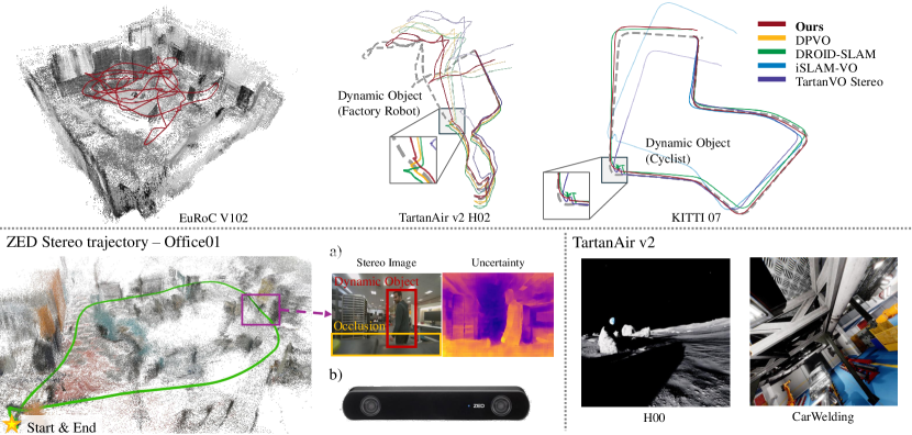
Figure 6: Top: Trajectories estimated by our model and baselines. We highlight the segments where dynamic objects interrupt the VO. Our method remains robust by implicitly filtering out unreliable features. Bottom left: We use our own platform with the ZED camera to collect data in the office. Our method demonstrates robustness against dynamic objects and visual occlusions in the images. Bottom right: samples of TartanAir v2 test dataset, which simulates the exotic lunar environment and factory with presence of dynamic objects.

In addition to quantitative evaluations, we conduct qualitative evaluations of our proposed system across multiple datasets including EuRoC, KITTI, and TartanAir v2, supplemented by manually collected data using a ZED stereo camera. Our model, even without multi-frame optimization, achieves top-tier performance and exhibits fewer glitches than baseline methods. As demonstrated in the Fig. 6, our method produces smoother trajectories and superior pose estimation precision. Fig. 6 a) presents that our model correctly identifies the region occluded by the mounted platform and dynamic objects in the scene and assigns a high uncertainty score to these regions.

Ablation Study   In Table. IV, we first perform the ablation study on each module of MAC-VO including (a. w/o CovKP & CovOPT) with random keypoint selector and identity covariance matrix. (b. w/o CovOpt) replace the metrics-aware covariance model with the identity covariance model. (c. w/o CovKP) replace the proposed keypoint selector with random keypoint selector.

To demonstrate the necessity of scale consistency and off-diagonal terms in our covariance model, we run the ablation study with different configurations: (I. DiagCov) remove off-diagonal terms in Eq. 3, (II. Scale-agnostic) normalize the covariance model by the average determinants of covariance matrices of each frame.

TABLE IV: Ablation study. Detailed results in Appendix. B-C.

Dataset	TartanAir v2 Hard		TartanAir v2 Easy
	$t_{\mathrm{rel}}$	$r_{\mathrm{rel}}$	$t_{\mathrm{rel}}$	$r_{\mathrm{rel}}$
Module Ablation
w/o CovKP & CovOpt	.0743	.5221	.0521	.2799
w/o CovOpt	.0679	.3776	.0511	.2367
w/o CovKP	.0188	.2347	.0066	.0808
Covariance Ablation
DiagCov	.0461	.3023	.0277	.1548
Scale Agnostic	.0204	.2321	.0086	.0764
Ours	.0141	.1429	.0051	.0670

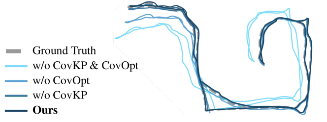
Figure 7: Results of various ablation setups on the trajectory H01 of TartanAir v2.

IV-C Runtime Analysis

The runtime analysis shown in Table. V uses the platform with AMD Ryzen 9 5950X CPU and NVIDIA 3090 Ti GPU. We also introduce a fast mode (MAC-VO Fast) that utilizes half-precision number in the network inference to enhance efficiency. This mode also speeds up the memory decoder network by reducing the number of iterative updates from 12 to 4. The fast mode performs at 10.5 fps (frames per second) with 70% of the performance of the original MAC-VO. More details are included in Appendix. C.

TABLE V: Time spent on each module of MAC-VO under different optimization with image resolution of $640\times 640$.

	Raw	TRT⋆	MP† + TRT⋆	MAC-VO Fast‡
Modules (ms)
Frontend Network	401.9	239.3	239.9	81.6
Optimization	53.4	57.5	-	-
Motion Model	5.2	5.1	5.3	5.2
Keypoint Selector	0.7	0.6	0.6	0.5
Covariance Model	0.6	0.7	0.7	0.7
Overall (fps)	2.15	3.25	3.96	10.57
⋆ TRT: TensorRT framework - https://developer.nvidia.com/tensorrt
† MP: multi-processing the PGO in parallel with the matching network.
‡ MAC-VO Fast: utilizes half-precision number (bf16) and light-weight model.

V Conclusion & Discussion

This paper proposes MAC-VO, a learning-based stereo VO method that leverages the metrics-aware covariance model. Our model outperforms most visual odometry and even SLAM algorithms on challenging datasets. In our current work, the model focuses on the two-frame pose optimization. We believe our accuracy will be further benefit from bundle adjustment, multi-frame optimization, and loop closure. Additionally, we are interested in exploring our metrics-aware covariance model in multi-sensor fusion, such as with IMUs.

Appendix A Covariance Model Formulation

A-A Depth Uncertainty From Disparity Uncertainty

In this section, we present the formulation for estimating the distribution of depth $\mathbf{d}$ on a single pixel given the estimated distribution of disparity ${\mathrm{Disp}}\sim\mathcal{N}(\mu_{{\mathrm{Disp}}},\sigma_{\mathrm{Disp}}^{2})$.

Following the pinhole camera model, the depth is calculated as $\mathbf{d}=bf_{x}/{\mathrm{Disp}}$ where the camera baseline is $b$. Since ${\mathrm{Disp}}$ can be zero, the distribution of $\mathbf{d}$ may be ill-defined. To fix this, we employ the first-order Taylor expansion to approximate $\mu_{d}$ and $\sigma_{d}^{2}$ such that $\mathbf{d}\sim\mathcal{N}(\mu_{d},\sigma_{d}^{2})$.

We assume the variance of disparity $\sigma_{{\mathrm{Disp}}}^{2}=(\gamma\mu_{\mathrm{Disp}})^{2}$ for some sufficiently small $\gamma>0$ such that the probability of ${\mathrm{Disp}}<=0$ is negligible. Based on this assumption, we have

$$\mu_{\mathbf{d}} =\mathbb{E}\Biggl{[}\frac{bf_{x}}{\mu_{\mathrm{Disp}}}+\left(\frac{d}{d\mu_{\mathrm{Disp}}}\frac{bf_{x}}{\mu_{\mathrm{Disp}}}\right)({\mathrm{Disp}}-\mu_{\mathrm{Disp}})\Biggr{.}$$ (6)

$$+\Biggl{.}\left(\frac{d^{2}}{d\mu_{\mathrm{Disp}}^{2}}\frac{bf_{x}}{\mu_{\mathrm{Disp}}}\right)\frac{({\mathrm{Disp}}-\mu_{\mathrm{Disp}})^{2}}{2}+\cdots\Biggr{]}$$

$$\approx\mathbb{E}\left[\frac{bf_{x}}{\mu_{\mathrm{Disp}}}\right]-\frac{1}{\mu_{\mathrm{Disp}}^{2}}\mathbb{E}[({\mathrm{Disp}}-\mu_{\mathrm{Disp}})]$$

$$=\frac{bf_{x}}{\mu_{\mathrm{Disp}}}-0=\frac{bf_{x}}{\mu_{\mathrm{Disp}}}$$

Similarly, $\sigma_{\mathbf{d}}^{2}$ can be expressed as

$$\sigma_{\mathbf{d}}^{2} =\mathrm{Var}\Biggl{[}\frac{bf_{x}}{\mu_{\mathrm{Disp}}}+\left(\frac{d}{d\mu_{\mathrm{Disp}}}\frac{bf_{x}}{\mu_{\mathrm{Disp}}}\right)({\mathrm{Disp}}-\mu_{\mathrm{Disp}})\Biggr{.}$$ (7)

$$+\Biggl{.}\left(\frac{d^{2}}{d\mu_{\mathrm{Disp}}^{2}}\frac{bf_{x}}{\mu_{\mathrm{Disp}}}\right)\frac{({\mathrm{Disp}}-\mu_{\mathrm{Disp}})^{2}}{2}+\cdots\Biggr{]}$$

$$\approx\mathrm{Var}\left[\frac{bf_{x}}{\mu_{\mathrm{Disp}}}+\left(\frac{d}{d\mu_{\mathrm{Disp}}}\frac{bf_{x}}{\mu_{\mathrm{Disp}}}\right)({\mathrm{Disp}}-\mu_{\mathrm{Disp}})\right]$$

$$=\left(\frac{bf_{x}}{\mu_{\mathrm{Disp}}^{2}}\right)^{2}\cdot\sigma_{\mathrm{Disp}}^{2}=\frac{(bf_{x}\gamma)^{2}}{\mu_{\mathrm{Disp}}^{2}}$$

Therefore, the approximation of depth uncertainty from disparity uncertainty is expressed as follows:

$$D\sim\mathcal{N}\left(\frac{bf_{x}}{\mu_{\mathrm{Disp}}},\frac{(bf_{x}\gamma)^{2}}{\mu_{\mathrm{Disp}}^{2}}\right)$$ (8)

Monte Carlo simulation indicates that for $\gamma<0.3$, the error of the aforementioned approximation is acceptable, as shown in Fig. 8.

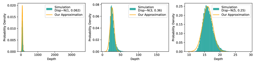
Figure 8: Result of Monte Carlo simulation on depth distribution. Despite the skewness in the simulated distribution, our approximation matches the simulation. As error rate $\gamma$ increases and average disparity ${\mathrm{Disp}}$ approaches $0$ (from right to left), the depth distribution becomes more skewed and the quality of approximation decreases.

A-B Depth Uncertainty with of Match Uncertainty

Let $q_{i,t}$ be the $i$-th keypoint on the camera plane at time $t$. Given the estimated optical flow $\mathbf{f}$ at $q_{i,t}$, the matched keypoint at time $t+1$ is defined as $q_{i,t+1}=q_{i,t}+\mathbf{f}_{i,t}$. Since $\mathbf{f}_{i,t}$ follows the gaussian distribution $\mathcal{N}(\hat{f}_{i,t},\hat{\Sigma}_{i,t})$, $q_{i,t+1}$ is a random variable following distribution of $\mathcal{N}(q_{i,t}+\hat{f}_{i,t},\hat{\Sigma}_{i,t})$.

Let $\varphi_{i,t}$ be a 2D Gaussian filter with covariance matrix $\hat{\Sigma}_{i,t}$, the probability for matched keypoint on some pixel $j$ is then expressed as $(\varphi_{i,t})_{j}$. Let $d_{j}$ denote the estimated depth at pixel $j$, then the average depth for pixel $q_{i,t+1}$ weighted by $\varphi$ is expressed as

$$\mu_{d_{i,t}}=\sum_{j}{(\varphi_{i,t})_{j}\cdot d_{j}},$$ (9)

and the estimated variance of depth of $q_{i,t+1}$ is calculated as weighted variance

$$\sigma_{d_{i,t}}^{2}=\sum_{j}{(\varphi_{i,t})_{j}\cdot(d_{j}-\mu_{d_{i,t}})^{2}}.$$ (10)

We could also model the depth of the matched point using a mixture of Gaussian distributions, but experiments show that this offers only a minimal performance improvement. Therefore, we use the straightforward weighted variance method to estimate depth uncertainty.

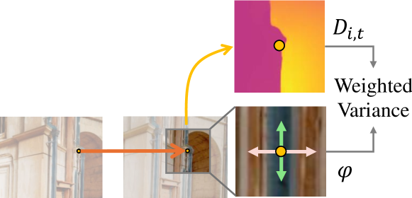
Figure 9: Estimate depth variance of the matched point under the presence of matching uncertainty

A-C Projecting 2D Uncertainty to Spatial Covariance

Let $\mathbf{u}_{i,t}\sim\mathcal{N}(u_{i,t},\sigma_{u_{i,t}}^{2})$, $\mathbf{v}_{i,t}\sim\mathcal{N}(v_{i,t},\sigma_{v_{i,t}}^{2})$, and $\mathbf{d}_{i,t}\sim\mathcal{N}(d_{i,t},\sigma_{d_{i,t}}^{2})$, we derive the distribution of 3D point under camera coordinate ${}^{c}\mathbf{p}_{i,t}=[\mathbf{x}_{i,t},\mathbf{y}_{i,t},\mathbf{z}_{i,t}]^{\top}\sim\mathcal{N}({}^{c}p_{i,t},{}^{c}\Sigma_{i,t})$.

Recall that the relationship between pixel coordinate $(\mathbf{u}_{i,t},\mathbf{v}_{i,t})$, depth $\mathbf{d}_{i,t}$ and 3D coordinate $\mathbf{x}_{i,t},\mathbf{y}_{i,t},\mathbf{z}_{i,t}$ is depicted as

$$\mathbf{x}_{i,t}=\frac{(\mathbf{u}_{i,t}-c_{x})\mathbf{d}_{i,t}}{f_{x}},\quad\mathbf{y}_{i,t}=\frac{(\mathbf{v}_{i,t}-c_{y})\mathbf{d}_{i,t}}{f_{y}},\quad\mathbf{z}_{i,t}=\mathbf{d}_{i,t}$$ (11)

Assume $\mathbf{u}_{i,t}$, $\mathbf{v}_{i,t}$, $\mathbf{d}_{i,t}$ are independent to each other, we have $\mathrm{Var}(\mathbf{u}_{i,t},\mathbf{d}_{i,t})=(\sigma_{u_{i,t}}^{2}+d_{i,t}^{2})(\sigma_{d_{i,t}}^{2}+u_{i,t}^{2})-u_{i,t}^{2}d_{i,t}^{2}$ [47]. Based on this expression of variance, it follows that

$$\sigma_{x_{i,t}}^{2} =\mathrm{Var}\left(\frac{\mathbf{u}_{i,t}\mathbf{d}_{i,t}}{f_{x}}-\frac{c_{x}\mathbf{d}_{i,t}}{f_{x}}\right)=\frac{\mathrm{Var}(\mathbf{u}_{i,t}\mathbf{d}_{i,t})}{f_{x}^{2}}+\frac{c_{x}^{2}\mathrm{Var}(\mathbf{d}_{i,t})}{f_{x}^{2}}$$ (12)

$$=\frac{(\sigma_{u_{i,t}}^{2}+d_{i,t}^{2})(\sigma_{d_{i,t}}^{2}+u_{i,t}^{2})-u_{i,t}^{2}d_{i,t}^{2}+c_{x}^{2}\sigma_{d_{i,t}}^{2}}{f_{x}^{2}}$$

$$\sigma_{y_{i,t}}^{2} =\mathrm{Var}\left(\frac{\mathbf{v}_{i,t}\mathbf{d}_{i,t}}{f_{y}}-\frac{c_{y}\mathbf{d}_{i,t}}{f_{y}}\right)=\frac{\mathrm{Var}(\mathbf{v}_{i,t}\mathbf{d}_{i,t})}{f_{y}^{2}}+\frac{c_{y}^{2}\mathrm{Var}(\mathbf{d}_{i,t})}{f_{y}^{2}}$$

$$=\frac{(\sigma_{v_{i,t}}^{2}+d_{i,t}^{2})(\sigma_{d_{i,t}}^{2}+v_{i,t}^{2})-v_{i,t}^{2}d_{i,t}^{2}+c_{y}^{2}\sigma_{d_{i,t}}^{2}}{f_{y}^{2}}$$

$$\sigma_{z_{i,t}}^{2} =\sigma_{d_{i,t}}^{2}$$

Under the assumption that $\mathbf{u}_{i,t},\mathbf{v}_{i,t},\mathbf{d}_{i,t}$ are independent to each other, we derive the covariance between $\mathbf{x}_{i,t}$, $\mathbf{y}_{i,t}$ and $\mathbf{z}_{i,t}$ as:

$$\mathrm{Cov}(\mathbf{x}_{i,t},\mathbf{y}_{i,t}) =\mathrm{Cov}\left(\frac{(\mathbf{u}_{i,t}-c_{x})\mathbf{d}_{i,t}}{f_{x}},\frac{(\mathbf{v}_{i,t}-c_{y})\mathbf{d}_{i,t}}{f_{y}}\right)$$ (13)

$$=\mathbb{E}\left[\frac{\mathbf{d}_{i,t}^{2}(\mathbf{u}_{i,t}-c_{x})(\mathbf{v}_{i,t}-c_{y})}{f_{x}f_{y}}\right]$$

$$-\mathbb{E}\left[\frac{(\mathbf{u}_{i,t}-c_{x})\mathbf{d}_{i,t}}{f_{x}}\right]\mathbb{E}\left[\frac{(\mathbf{v}_{i,t}-c_{y})\mathbf{d}_{i,t}}{f_{y}}\right]$$

$$=\frac{(\mathbb{E}[\mathbf{d}_{i,t}^{2}]-\mathbb{E}[\mathbf{d}_{i,t}]^{2})\mathbb{E}[\mathbf{u}_{i,t}-c_{x}]\mathbb{E}[\mathbf{v}_{i,t}-c_{y}]}{f_{x}f_{y}}$$

$$=\frac{\sigma_{d_{i,t}}^{2}}{f_{x}f_{y}}(u_{i,t}-c_{x})(v_{i,t}-c_{y})$$

and

$$\mathrm{Cov}(\mathbf{x}_{i,t},\mathbf{z}_{i,t}) =\mathrm{Cov}\left(\frac{(\mathbf{u}_{i,t}-c_{x})\mathbf{d}_{i,t}}{f_{x}},\mathbf{d}_{i,t}\right)$$ (14)

$$=\frac{(\mathbb{E}[\mathbf{d}_{i,t}^{2}]-\mathbb{E}[\mathbf{d}_{i,t}]^{2})\mathbb{E}[\mathbf{u}_{i,t}]}{f_{x}}=\frac{\sigma_{d_{i,t}}^{2}}{f_{x}}(u_{i,t}-c_{x})$$

$$\mathrm{Cov}(\mathbf{y}_{i,t},\mathbf{z}_{i,t}) =\mathrm{Cov}\left(\frac{(\mathbf{v}_{i,t}-c_{y})\mathbf{d}_{i,t}}{f_{y}},\mathbf{d}_{i,t}\right)$$

$$=\frac{(\mathbb{E}[\mathbf{d}_{i,t}^{2}]-\mathbb{E}[\mathbf{d}_{i,t}]^{2})\mathbb{E}[\mathbf{v}_{i,t}]}{f_{y}}=\frac{\sigma_{d_{i,t}}^{2}}{f_{y}}(v_{i,t}-c_{y})$$

Fig. 10 visualize the distribution of keypoints in 3D space via Monte Carlo and the 90% confidence interval of estimated distribution, confirming the necessity of off-diagonal terms.

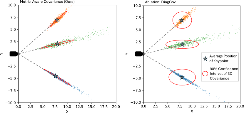
Figure 10: Comparison of proposed 3D covariance (left) and the diagonal covariance matrix (right, DiagCov in ablation study). Our method captures the uncertainty of keypoints significantly better than the diagonal covariance matrix.

Appendix B Additional Results

B-A Remaining Results on EuRoC, TartanAirv2, and KITTI

TABLE VI: Performance comparison of different methods on the EuRoC Dataset. Only even-ordered trajectory is shown here, see Table. I for the remaining results.

Trajectory	MH02		MH04		V101		V103		V202
	$t_{\mathrm{rel}}$	$r_{\mathrm{rel}}$	$t_{\mathrm{rel}}$	$r_{\mathrm{rel}}$	$t_{\mathrm{rel}}$	$r_{\mathrm{rel}}$	$t_{\mathrm{rel}}$	$r_{\mathrm{rel}}$	$t_{\mathrm{rel}}$	$r_{\mathrm{rel}}$
SLAM
ORB-SLAM 3	0.0036	0.0495	0.0061	0.0501	0.0049	0.0888	0.0137	0.2669	0.0090	0.1528
DROID-SLAM⋆	0.0012	0.0169	0.0031	0.0224	0.0024	0.0314	0.0036	0.0642	0.0017	0.0399
VO
TartanVO⋆†	0.0172	0.0621	0.0213	0.0681	0.0124	0.0756	0.0263	0.1552	0.0171	0.1251
TartanVO	0.0289	0.5037	0.0501	0.5400	0.0224	0.5322	0.0351	1.3127	0.0361	1.1607
iSLAM-VO	0.0041	0.0620	0.0082	0.0682	0.0041	0.0756	0.0088	0.1554	0.0078	0.1252
DPVO⋆†	0.0014	0.0212	0.0029	0.0264	0.0026	0.0405	0.0033	0.0662	0.0022	0.0493
Ours	0.0013	0.0199	0.0028	0.0273	0.0024	0.0304	0.0032	0.058	0.0018	0.0406
⋆ The estimated sequence is scale-aligned with ground truth.
† Monocular method.

TABLE VII: Relative motion error on the TartanAir v2 Hard Dataset. Only even numbered trajectories in the Hard subset are shown here. For odd-numbered trajectories in the Hard subset, see Table. VIII. ORB-SLAM3 lost track of all trajectories and is therefore not shown in the table.

Trajectory	H00		H02		H04		H06		H08		H10		H12
	$t_{\mathrm{rel}}$	$r_{\mathrm{rel}}$	$t_{\mathrm{rel}}$	$r_{\mathrm{rel}}$	$t_{\mathrm{rel}}$	$r_{\mathrm{rel}}$	$t_{\mathrm{rel}}$	$r_{\mathrm{rel}}$	$t_{\mathrm{rel}}$	$r_{\mathrm{rel}}$	$t_{\mathrm{rel}}$	$r_{\mathrm{rel}}$	$t_{\mathrm{rel}}$	$r_{\mathrm{rel}}$
SLAM
DROID-SLAM⋆	0.009	0.033	0.029	0.080	0.014	0.026	0.006	0.025	0.019	0.082	0.004	0.060	0.146	0.236
VO
iSLAM-VO	0.182	3.337	0.341	2.557	0.422	2.776	0.382	2.423	0.325	2.189	0.259	2.874	0.257	3.755
TartanVO⋆†	0.097	0.459	0.315	2.629	0.247	3.084	0.234	3.017	0.272	3.305	0.245	2.435	0.164	2.899
TartanVO	0.067	0.751	0.070	0.382	0.150	0.724	0.106	0.398	0.072	0.327	0.082	0.809	0.080	1.186
DPVO⋆†	0.010	0.077	0.025	0.079	0.308	0.654	0.024	0.066	0.054	0.254	0.164	0.250	0.189	1.430
Ours	0.011	0.120	0.008	0.058	0.033	0.168	0.017	0.090	0.016	0.085	0.011	0.162	0.027	0.604
⋆ The estimated sequence is scale-aligned with ground truth.
† Monocular method.

TABLE VIII: Performance comparison on the TartanAir v2 Easy Dataset.

Trajectory	E00		E01		E02		E03		E04		E05		E06		Avg.
	$t_{\mathrm{rel}}$	$r_{\mathrm{rel}}$	$t_{\mathrm{rel}}$	$r_{\mathrm{rel}}$	$t_{\mathrm{rel}}$	$r_{\mathrm{rel}}$	$t_{\mathrm{rel}}$	$r_{\mathrm{rel}}$	$t_{\mathrm{rel}}$	$r_{\mathrm{rel}}$	$t_{\mathrm{rel}}$	$r_{\mathrm{rel}}$	$t_{\mathrm{rel}}$	$r_{\mathrm{rel}}$	$t_{\mathrm{rel}}$	$r_{\mathrm{rel}}$
SLAM
ORB-SLAM3			.1019	2.349
DROID-SLAM⋆	.0077	.0144	.0025	.0199	.0063	.0409	.0049	.0251	.0009	.0147	.0031	.0463	.0016	.0235	.0039	.0264
VO
iSLAM-VO	.0656	.2873	.0456	.3853	.0359	.2234	.0508	.2635	.0268	.3201	.0464	.6624	.0362	.4606	.0439	.3718
TartanVO⋆†	.0532	.3237	.0937	.4750	.1066	.6048	.0756	.2230	.1114	.4032	.0862	.3185	.1373	.6620	.0949	.4300
TartanVO	.0505	.1334	.0322	.2078	.0237	.1105	.0303	.1417	.0173	.1681	.0279	.3828	.0218	.2329	.0291	.1967
DPVO⋆†	.0113	.0187	.0047	.0249	.0099	.0475	.0603	.2064	.0044	.0177	.0511	.0665	.0189	.1543	.0229	.0766
Ours	.0026	.0351	.0124	.1183	.0031	.0684	.0054	.0383	.0050	.0413	.0018	.0247	.0054	.1427	.0051	.0670
† Monocular method.  ⋆ Scale-aligned with ground truth.

TABLE IX: Performance comparison of different methods on the KITTI Dataset. Only odd-numbered trajectory is shown here, see Table. III for the remaining results.

Trajectory	01		03		05		07		09
	$t_{\mathrm{rel}}$	$r_{\mathrm{rel}}$	$t_{\mathrm{rel}}$	$r_{\mathrm{rel}}$	$t_{\mathrm{rel}}$	$r_{\mathrm{rel}}$	$t_{\mathrm{rel}}$	$r_{\mathrm{rel}}$	$t_{\mathrm{rel}}$	$r_{\mathrm{rel}}$
SLAM
ORB-SLAM 3	0.0416	0.0355	0.027	0.0425	0.0161	0.0416	0.0155	0.0385	0.0208	0.0444
DROID-SLAM⋆	0.7112	0.0406	0.0182	0.0385	0.0153	0.0353	0.0746	0.0734	0.0214	0.0378
VO
TartanVO⋆†	0.6834	0.0895	0.1234	0.0682	0.1821	0.0761	0.2005	0.0847	0.1704	0.1069
TartanVO	1.1408	0.2455	0.0477	0.0953	0.0637	0.0821	0.0700	0.0931	0.0990	0.1077
iSLAM-VO	0.2978	0.0896	0.0507	0.0681	0.0504	0.0758	0.0593	0.0842	0.0660	0.1064
DPVO⋆†	0.0942	0.0247	0.0302	0.0330	0.2221	0.0319	0.1064	0.0311	0.1723	0.0336
Ours	0.1670	0.1670	0.0504	0.0504	0.0466	0.0466	0.0507	0.0507	0.0567	0.0567
‡ Average is calculated over all trajectories (from 00 to 10) of KITTI.
⋆ The estimated sequence is scale-aligned with ground truth.
† Monocular method.

B-B Robustness Analysis

TABLE X: Robustness of systems on TartanAir v2 Hard test dataset demonstrate by the average variance of relative translation and rotation error.

Model	DROID-SLAM	iSLAM-VO	TartanVO⋆†	TartanVO	DPVO⋆†	Ours
Avg. $\sigma^{2}_{t_{\mathrm{rel}}}$	0.072	0.383	0.169	0.107	0.318	0.045
Avg. $\sigma^{2}_{r_{\mathrm{rel}}}$	0.418	2.925	2.748	0.991	2.099	0.475
⋆ The estimated sequence is scale-aligned with ground truth.
† Monocular method.

B-C Additional Ablation Study

TABLE XI: Performance comparison of different ablation setups on the TartanAir v2 Hard Dataset.

Relative Translation Error ($t_{\mathrm{rel}},\mathrm{m}/\mathrm{frame}$)
Trajectory	H00	H01	H02	H03	H04	H05	H06
System Modules
w/o CovKP & CovOpt	0.136	0.037	0.058	0.098	0.027	0.071	0.092
w/o CovOpt	0.171	0.033	0.061	0.106	0.023	0.034	0.048
w/o CovKP	0.025	0.005	0.015	0.025	0.005	0.029	0.028
Covariance Model
DiagCov	0.128	0.016	0.038	0.066	0.014	0.023	0.038
Scale Agnostic	0.041	0.004	0.018	0.027	0.005	0.021	0.027
Ours	0.008	0.034	0.005	0.015	0.009	0.005	0.020

Relative Rotation Error ($r_{\mathrm{rel}},{}^{\circ}/\mathrm{frame}$)
Trajectory	H00	H01	H02	H03	H04	H05	H06
System Modules
w/o CovKP & CovOpt	0.380	0.277	0.206	0.456	0.248	0.926	1.160
w/o CovOpt	0.350	0.244	0.248	0.507	0.176	0.449	0.669
w/o CovKP	0.099	0.042	0.076	0.247	0.059	0.629	0.491
Covariance Model
DiagCov	0.333	0.126	0.192	0.404	0.137	0.379	0.544
Scale Agnostic	0.173	0.042	0.098	0.253	0.060	0.500	0.498
Ours	0.102	0.145	0.063	0.078	0.141	0.055	0.465

TABLE XII: Performance comparison of different ablation setups on the TartanAir v2 Easy Dataset.

Relative Translation Error ($t_{\mathrm{rel}},\mathrm{m}/\mathrm{frame}$)
Trajectory	E00	E01	E02	E03	E04	E05	E06
System Modules
w/o CovKP & CovOpt	0.116	0.049	0.045	0.058	0.018	0.035	0.044
w/o CovOpt	0.124	0.052	0.048	0.070	0.016	0.020	0.027
w/o CovKP	0.010	0.003	0.006	0.008	0.002	0.009	0.009
Covariance Model
DiagCov	0.069	0.025	0.025	0.037	0.009	0.012	0.017
Scale Agnostic	0.026	0.004	0.006	0.009	0.002	0.005	0.008
Ours	0.003	0.012	0.003	0.005	0.005	0.002	0.005

Relative Rotation Error ($r_{\mathrm{rel}},{}^{\circ}/\mathrm{frame}$)
Trajectory	E00	E01	E02	E03	E04	E05	E06
System Modules
w/o CovKP & CovOpt	0.238	0.249	0.151	0.204	0.152	0.492	0.473
w/o CovOpt	0.219	0.254	0.187	0.275	0.132	0.278	0.313
w/o CovKP	0.048	0.031	0.039	0.058	0.025	0.189	0.174
Covariance Model
DiagCov	0.189	0.127	0.106	0.167	0.085	0.179	0.210
Scale Agnostic	0.073	0.033	0.027	0.067	0.029	0.148	0.136
Ours	0.035	0.118	0.068	0.038	0.041	0.025	0.143

B-D Datasets and Implementation

TartanAir dataset

The Tartanair dataset is a large-scale synthetic dataset encompassing highly diverse scenes, including various complex and challenging environments. Following the TartanAir data generation method, we created new, more diverse and challenging trajectories. From these, we selected that feature fast camera movements, low-light indoor environments, and simulated lunar surfaces lacking visual features. The images in the new dataset have a resolution of $640\times 640$ . When testing iSLAM-VO and TartanVO, we resized the input images to $448\times 640$ to match the input requirements of the optical flow network. Due to the substantial GPU memory required by DROID-SLAM for global bundle adjustment optimization when processing high-resolution images, we reduced the input image resolution to $512\times 512$ and manually reclaimed GPU and memory after testing each trajectory to avoid potential memory insufficiency.

KITTI dataset

The KITTI dataset is a well-known and widely used dataset for autonomous driving, containing detailed ground truth labels that make it suitable for evaluating the performance of various VO/SLAM methods. Learning-based methods may experience performance degradation when handling the image sizes in the KITTI dataset, therefore, we cropped the input images to different sizes based on the methods tested. Our model processed images cropped to $376\times 680$ , while for testing DROID-SLAM, the images were cropped to $320\times 832$ .

EuRoC dataset

The Euroc dataset consists of 11 trajectories collected by a drone and is also a widely used benchmark for VO/SLAM tasks. Some scenes in this dataset contain thousands of image pairs, which imposes computational pressure on DROID-SLAM when performing bundle adjustment. Thus, during testing, we reduced the input image resolution to $320\times 512$ and read every other frame of image pairs. In post-processing, we completed the entire trajectory by interpolating timestamps.

ZED Camera data

The ZED Camera data comprises real-world trajectory data captured using a ZED stereo camera, employed to test the robustness and generality of our model when faced with unseen data not present in the training set.

B-E Network and Training Details

In the uncertainty-aware matching network, we employ a flow decoder similar to Flowformer to obtain $\Delta f$. In each iteration, the flow $f_{x}$ is updated by $f_{x}\leftarrow f_{x}+\delta f$. With the shared features, we train a new decoder with ConvGRU layers to estimate the uncertainty updates $\Delta\Sigma$. To stabilize the training, we employ $\exp$ as the activation function of the covariance decoder.

For each pixel $x$, we extract the local cost-map patch $q_{x}$ from the cost map, and the context feature $t_{x}$ from the context encoder. We encode the $q_{x}$ using a transformer FFN. Given the 2D position $p=x+f_{x}$, we encode it into positional embedding $\text{PE}(p)$. We aggregate these features using CNN encoder ME to generate local motion features ${I_{x}}$. Utilizing the GMA module, the network’s global motion features $G_{x}$ are acquired from the current motion features $\text{Att}_{f}(t_{x})$ and ${I_{x}}$. Subsequently, the shared motion features $m_{x}$ is obtained by concatenating the $G_{x}$, $I_{x}$ and $\text{Att}(t_{x})$, where $\text{Att}(t_{x})$ is the attention of the context features. To estimate the flow update $\Delta f$ and $\Delta\Sigma$, we us the ConvGRU $\Sigma_{\pi}(m_{x})$

$$I_{x} =\text{ME}(f_{x},\text{Concat}(\text{FFN}(q_{x}),\text{PE}(p)))$$ (15)

$$G_{x} =\text{GMA}(\text{Att}(t_{x}),{I_{x}})$$

$$m_{x} =\text{Concat}(\text{Att}(t_{x}),{I_{x}},G_{x})$$

$$\Delta f =\text{FlowGRU}(m_{x})$$

$$\Delta\Sigma =\text{CovGRU}(m_{x})$$

We use AdamW optimizer with a learning rate of $12.5\times 10^{-5}$. The model is trained on A100 GPU consuming 16 GB GPU memory.

B-F GPU memory & Parameters

As shown in Table. XIII, we use 4.20GB of GPU memory, which is 6.7 times smaller than DROID-SLAM. This is because we utilize the sparse features for back-end optimization, reducing the requirements for the GPU memory.

TABLE XIII: The GPU memory consumption and the number of parameters during testing

Methods	GPU memory	Parameters
Ours	4.20GB	19.2M
TartanVO-stereo	1.16GB	47.3M
DROID-SLAM	28.34GB	4.0M
DPVO	1.51GB	3.4M

Appendix C Runtime Analysis

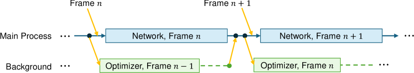
Figure 11: Multiprocessing setup places the optimizer in the background process and parallelizes the CPU-intensive (optimizer) and GPU-intensive (frontend network inference) jobs.

The runtime analysis use the platform with AMD Ryzen 9 5950X CPU and NVIDIA 3090 Ti GPU. To speed up the frontend network, we utilize CUDAGraph (CUDAGraph), TensorRT (TRT), and multi-processing (MP) to accelerate the original network (Raw). In our multiprocessing setup, as shown in Fig. B, a new CPU process is initiated to run the pose graph optimization in parallel with the front-end network, thereby maximizing GPU utilization.

We also introduce a fast mode (MAC-VO Fast) which utilizes half-precision (float16) number in the network inference to enhance computational efficiency. This mode also speeds up the memory decoder network by reducing the number of iterative updates from 12 to 4. The fast mode performs 10.5 fps (frames per second) with 70% of the performance of the original MAC-VO.

References

- [1] R. Mur-Artal, J. M. M. Montiel, and J. D. Tardos, “Orb-slam: a versatile and accurate monocular slam system,” IEEE transactions on robotics, vol. 31, no. 5, pp. 1147–1163, 2015.
- [2] W. Wang, Y. Hu, and S. Scherer, “Tartanvo: A generalizable learning-based vo,” 2020.
- [3] Z. Teed and J. Deng, “Droid-slam: Deep visual slam for monocular, stereo, and rgb-d cameras,” Advances in neural information processing systems, vol. 34, pp. 16 558–16 569, 2021.
- [4] Z. Teed, L. Lipson, and J. Deng, “Deep patch visual odometry,” Advances in Neural Information Processing Systems, vol. 36, 2024.
- [5] M. A. Fischler and R. C. Bolles, “Random sample consensus: a paradigm for model fitting with applications to image analysis and automated cartography,” Communications of the ACM, vol. 24, no. 6, pp. 381–395, 1981.
- [6] S. Zhao, H. Zhang, P. Wang, L. Nogueira, and S. Scherer, “Super odometry: Imu-centric lidar-visual-inertial estimator for challenging environments,” in 2021 IEEE/RSJ International Conference on Intelligent Robots and Systems (IROS). IEEE, 2021, pp. 8729–8736.
- [7] D. DeTone, T. Malisiewicz, and A. Rabinovich, “Superpoint: Self-supervised interest point detection and description,” in 2018 IEEE/CVF Conference on Computer Vision and Pattern Recognition Workshops (CVPRW). IEEE, Jun. 2018. [Online]. Available: http://dx.doi.org/10.1109/CVPRW.2018.00060
- [8] E. Rublee, V. Rabaud, K. Konolige, and G. Bradski, “Orb: An efficient alternative to sift or surf,” in 2011 International Conference on Computer Vision, 2011, pp. 2564–2571.
- [9] D. G. Lowe, “Distinctive image features from scale-invariant keypoints,” Int. J. Comput. Vision, vol. 60, no. 2, p. 91–110, nov 2004. [Online]. Available: https://doi.org/10.1023/B:VISI.0000029664.99615.94
- [10] S. Wang, V. Leroy, Y. Cabon, B. Chidlovskii, and J. Revaud, “Dust3r: Geometric 3d vision made easy,” arXiv preprint arXiv:2312.14132, 2023.
- [11] Z. Huang, X. Shi, C. Zhang, Q. Wang, K. C. Cheung, H. Qin, J. Dai, and H. Li, “Flowformer: A transformer architecture for optical flow,” in European conference on computer vision. Springer, 2022, pp. 668–685.
- [12] S. Jiang, D. Campbell, Y. Lu, H. Li, and R. Hartley, “Learning to estimate hidden motions with global motion aggregation,” in Proceedings of the IEEE/CVF international conference on computer vision, 2021, pp. 9772–9781.
- [13] G. Klein and D. Murray, “Parallel tracking and mapping for small ar workspaces,” in 2007 6th IEEE and ACM international symposium on mixed and augmented reality. IEEE, 2007, pp. 225–234.
- [14] R. Wang, M. Schworer, and D. Cremers, “Stereo dso: Large-scale direct sparse visual odometry with stereo cameras,” in Proceedings of the IEEE international conference on computer vision, 2017, pp. 3903–3911.
- [15] J. Engel, T. Schöps, and D. Cremers, “Lsd-slam: Large-scale direct monocular slam,” in European conference on computer vision. Springer, 2014, pp. 834–849.
- [16] X. Gao, R. Wang, N. Demmel, and D. Cremers, “Ldso: Direct sparse odometry with loop closure,” in International Conference on Intelligent Robots and Systems (IROS), October 2018.
- [17] J. Civera, A. J. Davison, and J. M. M. Montiel, “Inverse depth parametrization for monocular slam,” IEEE Transactions on Robotics, vol. 24, no. 5, pp. 932–945, 2008.
- [18] J. M. M. Montiel, J. Civera, and A. J. Davison, “Unified inverse depth parametrization for monocular slam,” in Robotics: Science and Systems, 2006. [Online]. Available: https://api.semanticscholar.org/CorpusID:18457284
- [19] T. Qin, P. Li, and S. Shen, “Vins-mono: A robust and versatile monocular visual-inertial state estimator,” IEEE Transactions on Robotics, vol. 34, no. 4, pp. 1004–1020, 2018.
- [20] S. Yang and S. Scherer, “Cubeslam: Monocular 3-d object slam,” IEEE Transactions on Robotics, vol. 35, no. 4, pp. 925–938, 2019.
- [21] Y. Qiu, C. Wang, W. Wang, M. Henein, and S. Scherer, “Airdos: Dynamic slam benefits from articulated objects,” in 2022 International Conference on Robotics and Automation (ICRA). IEEE, 2022, pp. 8047–8053.
- [22] Z. Teed and J. Deng, “Raft: Recurrent all-pairs field transforms for optical flow,” in Computer Vision–ECCV 2020: 16th European Conference, Glasgow, UK, August 23–28, 2020, Proceedings, Part II 16. Springer, 2020, pp. 402–419.
- [23] C. M. Parameshwara, G. Hari, C. Fermüller, N. J. Sanket, and Y. Aloimonos, “Diffposenet: Direct differentiable camera pose estimation,” in Proceedings of the IEEE/CVF Conference on Computer Vision and Pattern Recognition, 2022, pp. 6845–6854.
- [24] P.-E. Sarlin, D. DeTone, T. Malisiewicz, and A. Rabinovich, “Superglue: Learning feature matching with graph neural networks,” in Proceedings of the IEEE/CVF conference on computer vision and pattern recognition, 2020, pp. 4938–4947.
- [25] T. Zhou, M. Brown, N. Snavely, and D. G. Lowe, “Unsupervised learning of depth and ego-motion from video,” in Proceedings of the IEEE conference on computer vision and pattern recognition, 2017, pp. 1851–1858.
- [26] R. Li, S. Wang, Z. Long, and D. Gu, “Undeepvo: Monocular visual odometry through unsupervised deep learning,” in 2018 IEEE international conference on robotics and automation (ICRA). IEEE, 2018, pp. 7286–7291.
- [27] K. Tateno, F. Tombari, I. Laina, and N. Navab, “Cnn-slam: Real-time dense monocular slam with learned depth prediction,” in Proceedings of the IEEE conference on computer vision and pattern recognition, 2017, pp. 6243–6252.
- [28] G. Costante, M. Mancini, P. Valigi, and T. A. Ciarfuglia, “Exploring representation learning with cnns for frame-to-frame ego-motion estimation,” IEEE robotics and automation letters, vol. 1, no. 1, pp. 18–25, 2015.
- [29] E. Dexheimer and A. J. Davison, “Learning a depth covariance function,” in 2023 IEEE/CVF Conference on Computer Vision and Pattern Recognition (CVPR). IEEE, Jun. 2023, p. 13122–13131. [Online]. Available: http://dx.doi.org/10.1109/CVPR52729.2023.01261
- [30] X. Nie, D. Shi, R. Li, Z. Liu, and X. Chen, “Uncertainty-aware self-improving framework for depth estimation,” IEEE Robotics and Automation Letters, vol. 7, no. 1, pp. 41–48, 2022.
- [31] A. S. Wannenwetsch, M. Keuper, and S. Roth, “Probflow: Joint optical flow and uncertainty estimation,” in Proceedings of the IEEE International Conference on Computer Vision (ICCV), Oct 2017.
- [32] N. Yang, L. v. Stumberg, R. Wang, and D. Cremers, “D3vo: Deep depth, deep pose and deep uncertainty for monocular visual odometry,” in Proceedings of the IEEE/CVF conference on computer vision and pattern recognition, 2020, pp. 1281–1292.
- [33] T. Fu, S. Su, Y. Lu, and C. Wang, “islam: Imperative slam,” IEEE Robotics and Automation Letters, 2024.
- [34] A. Ranjan, V. Jampani, L. Balles, K. Kim, D. Sun, J. Wulff, and M. J. Black, “Competitive collaboration: Joint unsupervised learning of depth, camera motion, optical flow and motion segmentation,” in Proceedings of the IEEE/CVF conference on computer vision and pattern recognition, 2019, pp. 12 240–12 249.
- [35] P.-E. Sarlin, A. Unagar, M. Larsson, H. Germain, C. Toft, V. Larsson, M. Pollefeys, V. Lepetit, L. Hammarstrand, F. Kahl, and T. Sattler, “Back to the feature: Learning robust camera localization from pixels to pose,” in 2021 IEEE/CVF Conference on Computer Vision and Pattern Recognition (CVPR). IEEE, Jun. 2021. [Online]. Available: http://dx.doi.org/10.1109/CVPR46437.2021.00326
- [36] G. Costante and M. Mancini, “Uncertainty estimation for data-driven visual odometry,” IEEE Transactions on Robotics, vol. 36, no. 6, pp. 1738–1757, 2020.
- [37] D. Muhle, L. Koestler, K. Jatavallabhula, and D. Cremers, “Learning correspondence uncertainty via differentiable nonlinear least squares,” in Proceedings of the IEEE/CVF Conference on Computer Vision and Pattern Recognition, 2023, pp. 13 102–13 112.
- [38] N. Kaygusuz, O. Mendez, and R. Bowden, “Mdn-vo: Estimating visual odometry with confidence,” in 2021 IEEE/RSJ International Conference on Intelligent Robots and Systems (IROS). IEEE, Sep. 2021. [Online]. Available: http://dx.doi.org/10.1109/IROS51168.2021.9636827
- [39] P. Lindenberger, P.-E. Sarlin, V. Larsson, and M. Pollefeys, “Pixel-perfect structure-from-motion with featuremetric refinement,” in 2021 IEEE/CVF International Conference on Computer Vision (ICCV). IEEE, Oct. 2021. [Online]. Available: http://dx.doi.org/10.1109/ICCV48922.2021.00593
- [40] R. L. Russell and C. Reale, “Multivariate uncertainty in deep learning,” IEEE Transactions on Neural Networks and Learning Systems, vol. 33, no. 12, pp. 7937–7943, 2021.
- [41] A. N. Angelopoulos and S. Bates, Conformal Prediction: A Gentle Introduction. Now Foundations and Trends, 2023.
- [42] Y. Qiu, C. Wang, C. Xu, Y. Chen, X. Zhou, Y. Xia, and S. Scherer, “Airimu: Learning uncertainty propagation for inertial odometry,” 2023.
- [43] W. Wang, D. Zhu, X. Wang, Y. Hu, Y. Qiu, C. Wang, Y. Hu, A. Kapoor, and S. Scherer, “Tartanair: A dataset to push the limits of visual slam,” 2020.
- [44] C. Wang, D. Gao, K. Xu, J. Geng, Y. Hu, Y. Qiu, B. Li, F. Yang, B. Moon, A. Pandey et al., “Pypose: A library for robot learning with physics-based optimization,” in IEEE/CVF Conference on Computer Vision and Pattern Recognition (CVPR), 2023, pp. 22 024–22 034.
- [45] M. Burri, J. Nikolic, P. Gohl, T. Schneider, J. Rehder, S. Omari, M. W. Achtelik, and R. Siegwart, “The euroc micro aerial vehicle datasets,” The International Journal of Robotics Research, vol. 35, no. 10, pp. 1157–1163, 2016. [Online]. Available: https://doi.org/10.1177/0278364915620033
- [46] A. Geiger, P. Lenz, and R. Urtasun, “Are we ready for autonomous driving? the kitti vision benchmark suite,” in Conference on Computer Vision and Pattern Recognition (CVPR), 2012.
- [47] L. A. Goodman, “On the exact variance of products,” Journal of the American Statistical Association, vol. 55, no. 292, pp. 708–713, 1960. [Online]. Available: https://www.tandfonline.com/doi/abs/10.1080/01621459.1960.10483369