MALADY: Multiclass Active Learning with Auction Dynamics on Graphs

Abstract

Active learning enhances the performance of machine learning methods, particularly in semi-supervised cases, by judiciously selecting a limited number of unlabeled data points for labeling, with the goal of improving the performance of an underlying classifier. In this work, we introduce the Multiclass Active Learning with Auction Dynamics on Graphs (MALADY) framework which leverages the auction dynamics algorithm on similarity graphs for efficient active learning. In particular, we generalize the auction dynamics algorithm on similarity graphs for semi-supervised learning in [24] to incorporate a more general optimization functional. Moreover, we introduce a novel active learning acquisition function that uses the dual variable of the auction algorithm to measure the uncertainty in the classifier to prioritize queries near the decision boundaries between different classes. Lastly, using experiments on classification tasks, we evaluate the performance of our proposed method and show that it exceeds that of comparison algorithms.

Keywords: Active Learning, Auction Dynamics for Semi-Supervised Learning, Uncertainty Sampling

1 Introduction

The choice of training points can have a significant impact on the performance of a machine learning model, particularly in semi-supervised learning (SSL) scenarios where the training set is small. Active learning is a sub-field of machine learning that improves the performance of underlying machine learning methods by carefully selecting unlabeled points to be labeled via the use of a human in the loop or domain expert.

Most active learning methods alternate between (1) training a model using current labeled information and (2) selecting query points from an unlabeled set using an acquisition function that quantifies the utility of each point in the unlabeled set. This iterative process of training a classifier and labeling chosen query points is referred to as the active learning process, whose flowchart is shown in Figure 1. Given a dataset $\mathcal{X}=\{x_{1},x_{2},\ldots,x_{N}\}\subset\mathbb{R}^{d}$, we define the labeled set $\mathcal{L}\subset\mathcal{X}$ as the set of points for which we have observed their corresponding labels $y_{i}=y(x_{i})\in\{1,2,\ldots,C\}$; then, by labeled data, we refer to both the labeled set $\mathcal{L}$ of inputs along with their corresponding labels $\{y_{i}\}_{x_{i}\in\mathcal{L}}$. The unlabeled set then is the set of unlabeled inputs, $\mathcal{U}=\mathcal{X}\setminus\mathcal{L}$. A query set $\mathcal{Q}\subset\mathcal{U}$ then is the set of unlabeled points that have been chosen to be labeled and added to the labeled set for the next iteration of the active learning process. While the sets $\mathcal{L}$ and $\mathcal{U}$ change throughout the active learning process as query points are labeled, we simplify our notation of these sets to not explicitly denote the iteration; rather, $\mathcal{L},\ \mathcal{U},$ and $\mathcal{Q}$ will respectively denote the labeled, unlabeled, and query sets at the current iteration of the active learning process.

Given the current $\mathcal{L}$ and $\mathcal{U}$, the main challenge in active learning is to design an acquisition function $\mathcal{A}:\mathcal{U}\rightarrow\mathbb{R}$ that quantifies the benefit of obtaining the label for each currently unlabeled point. The acquisition functions values $\mathcal{A}(x)$ for each $x\in\mathcal{U}$ then allows one to prioritize which currently unlabeled data points are chosen to be in the query set $\mathcal{Q}$ to in turn be labeled. When $|\mathcal{Q}|=1$ it is referred to as sequential active learning while $|\mathcal{Q}|>1$ corresponds to batch active learning. While there are various ways to practically select $\mathcal{Q}\subset\mathcal{U}$ from the set of acquisition function values $\{\mathcal{A}(x)\}_{x\in\mathcal{U}}$, it is most common in sequential active learning to select $\mathcal{Q}=\{x^{\ast}\}$ where $x^{\ast}=\operatorname*{arg\,max}_{x\in\mathcal{U}}\mathcal{A}(x)$ is the maximizer of the acquisition function.

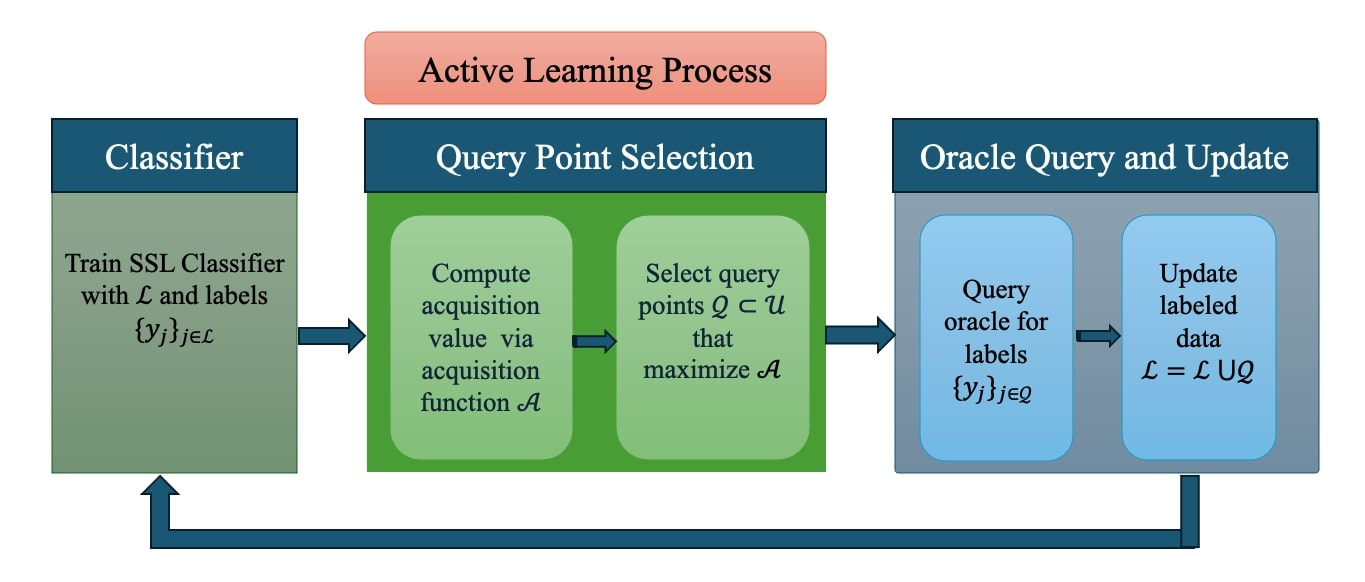
Figure 1: Visual description of the active learning process: The process starts by training the underlying classifier using the initial labeled set $\mathcal{L}$. Query points $\mathcal{Q}\in\mathcal{U}$ are then selected based on the current acquisition function value. These query points are also labeled according to an oracle (human in the loop or a domain expert) and subsequently the points are added to the current labeled data $\mathcal{L}$. This process continues until the desired number of points is reached in the labeled set $\mathcal{L}$.

An important component of the active learning process is the underlying method used for training a classifier based on the currently labeled data, $\mathcal{L}$. To this end, (similarity) graph-based methods have proven to be effective models for semi-supervised and active learning settings, particularly in the low label rate regime [46, 12, 13]. These methods leverage both the labeled and unlabeled sets to construct a similarity graph on which the observed labels on $\mathcal{L}$ are used to make inferences of the labels on the unlabeled data according to the graph topology; in this way, the geometric structure of the dataset is modeled with the graph and similar data points receive similar inferred outputs. In contrast, variants of auction algorithms, originally developed by Bertsekas [8, 9, 10, 7] for solving the classic assignment problem, have a simple intuitive structure, are easy to code, and have excellent performance. In this paper, we integrate (similarity) graph-based techniques and auction-based procedures to derive the underlying algorithm for training the classifier used in the active learning process.

In [24], the authors have shown how auction algorithms can be utilized for various applications such as semi-supervised graph-based learning and data classification in the presence of equality or inequality class size constraints on the individual classes. Modifications of this technique for the classification of 3D sensory data are discussed in [30]. Moreover, auction algorithms can be utilized in Merriman, Bence,and Osher (MBO)-based threshold dynamics schemes, which involve threshold dynamics to tackle different tasks; this was shown in [24]. For example, the original MBO scheme [35] was developed in 1992 to simulate and approximate motion by mean curvature; the procedure consists of alternating between diffusion and thresholding. Such an MBO technique was then modified and adapted to a similarity graph setting for the purpose of binary classification and image inpainting in [33], with a multiclass extension developed in [22] and [32]. Applications of the graph-based technique to heat kernel pagerank and hyperspectral imagery and video were detailed in [31] and [34], respectively. A summary of recent graph-based optimization approaches for machine learning, include MBO-based techniques was presented in [6].

Uncertainty sampling-based acquisition functions [44, 5, 42] are one of the most popular and computationally efficient acquisition functions in practice. In particular, an uncertainty-based acquisition function favors unlabeled points that are near a decision boundary and are most ”uncertain” for classification. These methods are emblematic of exploitative active learning since they explicitly use measures of distances to decision boundaries to select query points [38]. Moreover, some of the acquisition functions designed for graph-based classifiers include Uncertainty Norm for Poisson Reweighted Laplace Learning [38], Variance Minimization (VOpt) [25], Model-Change (MC) [37, 36], model-change variance optimal (MCVOpt) [37, 36], $\Sigma$-optimality [29], hierarchical sampling for active learning [20], Cautious Active Clustering [17], and Shortest-Shortest path $S^{2}$ [19].

With regards to active learning for graph-based semi-supervised classifiers, various recent pipelines have been developed for image processing applications including image segmentation [16], surface water and sediment detection [15], classification of synthetic aperture radar (SAR) data [39, 14], unsupervised clustering of hyperspectal images using nonlinear diffusion [40], and hyperspectral unmixing [15].

Lastly, acquisition functions for active learning have also been integrated in deep learning frameworks to boost the performance of such parametric models. In particular, some of the recent works include batch active learning by diverse gradient embeddings (BADGE) [4], active learning framework in Bayesian deep learning [21], diverse batch acquisition for deep Bayesian active learning [27], diffusion-based deep active learning [28], stochastic batch acquisition functions [26], and active learning for convolutional neural networks [43].

In this paper, we consider a more general formulation and algorithm than was considered in [24] and [30] and integrate active learning components to develop MALADY, an accurate active learning algorithm incorporating auction dynamics on graphs.

The contributions of the paper are summarized as follows:

• We generalize the auction dynamics algorithm for semi-supervised learning [24] by incorporating a more general optimization energy functional. The general formulation can be reformulated as a series of modified assignment problems, each of which can be tackled using auction algorithms incorporating volume constraints. This serves as the underlying semi-supervised classifier for our active learning process.

• We propose a novel acquisition function for active learning that uses the dual variables of the dual formulation of the modified assignment problem incorporating upper and lower bound class size constraints. The proposed acquisition function (i) measures the uncertainty of the volume bound auction algorithm for graph-based semi-supervised problems and (ii) captures salient geometric classifier info that can be leveraged for exploitation of decision boundaries.

• We conduct experiments on data classification using various datasets, and the results demonstrate that our proposed framework performs more accurately compared to other state-of-the-art methods.

The remainder of the paper is organized as follows: in Section 2, we present background information on the graph-based framework and the auction algorithm with volume constraints. In Section 3, we derive our semi-supervised classifier and the proposed acquisition function. The results of the experiments on benchmark data sets and the discussion of the results are presented in Section 4. Section 5 provides concluding remarks.

2 Background

In this section, we first discuss the (similarity) graph construction technique which is fundamental for graph-based methods. Then, we discuss auction dynamics with volume constraints for semi-supervised learning [24] as the technique is fundamental for the construction of our proposed semi-supervised method. The last subsection reviews some semi-supervised learning methods using auction procedures.

2.1 Graph Construction

In this section, we review the graph-based framework we used in this paper. Consider a dataset $X=\{x_{1},x_{2},\cdots x_{N}\}\in\mathbb{R}^{d}$, where each data element is represented by a $d$-dimensional feature vector. We generate a undirected graph $G(X,W)$ of vertices and edges between vertices, where $X$ is set of vertices representing data elements, and $W\in\mathbb{R}^{N\times N}$ is the weight matrix, consisting of weights between pairs of vertices. The weight matrix is computed using a weight function $W:X\times X\rightarrow\mathbb{R}$, where $W_{i,j}$ denotes the weight on the edge between the vertices $x_{i}$, $x_{j}$, $i\neq j$. Overall, the weight matrix quantifies the similarities between the features vectors, i.e. data elements, thus, the graph-based framework is able to provide crucial information about the data. Some popular weight functions include:

• the Gaussian weight function

  $$w(x_{i},x_{j})=\exp\left(-\frac{d(x_{i},x_{j})^{2}}{\sigma^{2}}\right),$$ (1)

  
  

  where $d(x_{i},x_{j})$ represents a distance (computed using a measure) between vertices $x_{i}$ and $x_{j}$, associated with the $i^{th}$ and $j^{th}$ data elements, and $\sigma>0$ is a parameter which controls scaling in the weight function.

• the Zelnik-Manor and Perona (ZMP) weight function [47]

  $$w(x_{i},x_{j})=\exp\left(-\frac{d(x_{i},x_{j})^{2}}{\sigma(x)\sigma(y)}\right),$$ (2)

  
  

  where $d(x_{i},x_{j})$ represents a distance metric and $\sqrt{\sigma(x_{i})}=d(x_{i},x_{M})$ is a local parameter for each $x_{i}$, where $x_{M}$ is the $M^{th}$ closest vector to $x_{i}$.

• cosine similarity weight function [45]

  $$w(x_{i},x_{j})=\exp\left(-\frac{d(x_{i},x_{j})^{2}}{\sigma(x)\sigma(y)}\right),$$ (3)

  where $d(x_{i},x_{j})=arccos\left(\frac{\langle x_{i},x_{j}\rangle}{||x_{i}||||x_{j}||}\right)$ and $\sqrt{\sigma(x_{i})}=d(x_{i},x_{M})$ is a local parameter for each $x_{i}$, and $x_{M}$ is the $M^{th}$ closest vector to $x_{i}$.

With the assumption that the high dimensional data is concentrated near a low dimensional manifold and the manifold is locally Euclidean, we only compute the $k$ nearest neighbors (KNN) of each of the points using an approximate nearest neighbor search algorithm. This ensures that the weight matrix is a sparse matrix and enhances the computational efficiency of our algorithm. To compute the weight matrix, we use the Graph Learning package [12] which uses the Annoy library [1] for an approximate nearest neighbor search. To preserve the symmetric property of the weight matrix, we calculate the final weight matrix as $W_{final}(x_{i},x_{j})=\{W(x_{i},x_{j})+W(x_{j},x_{i})\}/2$.

2.2 Auction Algorithm with Exact Volume Constraints

Given two disjoint sets $X$ and $Y$ of same cardinality $r$ and a cost function $c:X\times Y\rightarrow\mathbb{R}$, the assignment problem aims to identify a one-to-one correspondence $M=\{(x_{1},y_{1}),\cdots,(x_{r},y_{r})\}$ of the sets $X$ and $Y$, such that the total cost of the matching

$$\sum_{(x,y)\in M}c(x_{i},y_{j})$$ (4)

is maximized. The assignment problem (4) can be restated as the following optimization problem by representing the matching as a binary vector $z$, where $z_{y}(x)=1$ if $(x,y)$ are matched and $0$ otherwise:

$$\max_{\mathbf{z}:X\times Y\to\{0,1\}}\sum_{x\in X}\sum_{y\in Y}c(x,y)z_{y}(x)\quad\textrm{s.t.}\;\sum_{x\in X}z_{y}(x)=1,\sum_{y\in Y}z_{y}(x)=1.$$ (5)

Moreover, the above optimization problem can be written as a classical linear programming problem ($LP$) if we relax the binary constraint on $\bm{z}$:

$$\max_{\bm{z\geq 0}} \sum_{x\in X}\sum_{y\in Y}c(x,y)z_{y}(x)\hskip 14.22636pt\textrm{s.t.}\quad \sum_{x\in X}z_{y}(x)=1, \hskip 8.5359pt\sum_{y\in Y}z_{y}(x)=1.\hskip 14.22636pt(LP)$$ (6)

Furthermore, we can split $Y$ into $N$ similarity classes $\{S_{i}\}_{i=1}^{N}$ each of size $\{V_{i}\}$, and let $c(x,y)=a_{i}(x)$ for each $y\in S_{i}$. With this choices, we can reformulate (6) into:

$$\max_{\bm{z\geq 0}} \sum_{x\in X}\sum_{i=1}^{N}a_{i}(x)\sum_{y\in S_{i}}z_{y}(x)\hskip 14.22636pt\textrm{s.t.}\quad \sum_{x\in X}z_{y}(x)=1, \hskip 8.5359pt\sum_{y\in Y}z_{y}(x)=1\hskip 14.22636pt$$ (7)

By setting $u_{i}(x)=\sum_{y\in S_{i}}z_{y}(x)$, we obtain the equivalent problem

$$\max_{\bm{u\geq 0}} \sum_{x\in X}\sum_{i=1}^{N}a_{i}(x)u_{i}(x)\hskip 14.22636pt\textrm{s.t.}\quad \sum_{x\in X}u_{i}(x)=S_{i}, \hskip 8.5359pt\sum_{i=1}^{N}u_{i}(x)=1\hskip 14.22636pt.$$ (8)

We will focus on solving (8) which is a special case of (6). First, it is helpful to practically interpret (8). In particular, one can view each class as an institution, such as a gym, that offers a certain number of memberships and the data elements as people trying to obtain a deal on buying only one of the objects. Moreover, the coefficients $a_{i}(x)$ represent person $x$’s desire to buy the membership in institution $i$. The solution to (8) maximizes the total satisfaction of the population. Notice that the class size constraints (i.e. number of memberships available) make the assignment of institution memberships to people nontrivial.

One approach to (8) involves the market mechanism. In this case, an institution $j$ is equipped with a price $p_{j}$. Then, person $x$ will want buy the membership from an institution that offers the best value:

$$j^{*}(x)=\operatorname*{arg\,max}_{1\leq j\leq N}\hskip 2.84544pta_{j}(x)-p_{j}$$ (9)

The challenge is to compute an optimal price vector, called an equilibrium price vector, that results in an institution-person matching which satisfies the constraints on the number of available memberships. The answer lies in the dual formulation of the assignment problem, which can be shown to be the following problem:

$$\min_{\bm{p}\in\mathbb{R}^{n},\bm{\pi}\in\mathbb{R}^{n}} \sum_{i=1}^{N}p_{i}S_{i}+\sum_{x}\bm{\pi}(x)$$ (10)

subject to $$\bm{\pi}(x)+p_{i}\geq a_{i}(x).$$

It turns out that the equilibrium price vector $p_{*}$ of primal problem is in fact the optimal solution of dual problem (10). Moreover, the optimal value of $\bm{\pi}$ is completely determined by $\bm{p}$: given a price vector $\bm{p}$, the above dual problem is minimized when $\pi(x)$ equals the maximum value of $a_{i}(x)-p_{i}$ over $i$.

According to complementary slackness (CS) condition, a complete assignment $M$ and a price vector $p$ are primal and dual optimal if and only if each person is assigned to an institution offering the best deal to them. Moreover, the CS condition can be relaxed to allow a person to be assigned to institutions that are within $\epsilon$ of achieving the best deal to them in the definition (9). In particular, we say that an assignment $M$ and a price vector $\bm{p}$ satisfies $\epsilon$-complementary slackness ($\epsilon$-CS) if

$$\pi(x)-\epsilon\leq\hskip 2.84544pta_{i}(x)-p_{i}\;\;\text{for all}\;\;i.$$ (11)

In [8], Bertsekas detailed an auction algorithm technique to solve the assignment problem by finding the equilibrium (optimal) price vector. Since the original seminal paper, Bertsekas and others have extended the technique to more general problems and have improved the computational aspects of the procedure. For example, [10] develops a technique that efficiently handles assignment problems with multiple identical objects. Overall, an exhaustive reference on auction algorithms is included in [9] which contains information on linear network optimization and [7] on network optimization.

Bertsekas’ auction technique is the following: at the beginning of an iteration we start with an assignment and price vector satisfying $\epsilon$-CS with $\epsilon>0$. There are two phases in each iteration: the bidding phase and assignment phase. In each iteration, the assignment $M$ and price vector $\bm{p}$ is updated while maintaining $\epsilon$-CS. The two phases are described below:

• Bidding phase: For each data element $x$, under the assignment $M$:

  • Compute the current value $v_{i}=a_{i}(x)-p_{i}$ for each class $i$, and choose $i^{*}$ such that $i^{*}\in\operatorname*{arg\,max}v_{i}$.

  • Find the best value offered by a class other than $i^{*}$:

    $$u_{i}=\operatorname*{arg\,max}_{i\neq i^{*}}v_{i}.$$ (12)

  • Compute the bid $b(x)$ of data element $x$ for class $i^{*}$ given by

    $$b(x)=p_{i^{*}}+\epsilon+v_{i^{*}}-u_{i}$$ (13)

• Assignment phase:

  • If class $i^{*}$ has already given out $V_{i^{*}}$ memberships, remove the person $y$ currently assigned to the class with the lowest bid and add $x$ to class $i^{*}$, and set $p_{i^{*}}$ to be the minimum bid value over all people currently assigned to class $i^{*}$.

  • If class $i^{*}$ has not yet given out all $V_{i^{*}}$ memberships, add $x$ to class $i^{*}$. If now all memberships of class $i^{*}$ are bought, set $p_{i^{*}}$ to be the minimum bid value over all people currently assigned to class $i^{*}$.

The Membership Auction algorithm described above is given in Appendix as Algorithm 3.

2.3 Auction Algorithm with Upper and Lower Bound Volume Constraints

In [24], the authors presented a upper and lower bound auction algorithm for semi-supervised learning that allows the size of each class to fluctuate between upper and lower bounds. In particular, let $N$ be the number of classes, and suppose that class $j$ must have at least $B_{j}$ members and at most $U_{j}$ members, where $B_{j}\leq U_{j}$, and $\sum_{1}^{N}B_{j}\leq n\leq\sum_{j=1}^{N}U_{j}$.

With these additional constraints, the modified version of the assignment problem becomes:

$$\max_{u\geq 0}\sum_{x}\sum_{i=1}^{N}a_{i}(x)u_{i}(x)\hskip 14.22636pt\textrm{s.t.}\quad\sum_{i=1}^{N}u_{i}(x)=1,\;B_{i}\leq\sum_{x}u_{i}(x)\leq U_{i}\;\;\forall i.$$ (14)

The addition of these bounds in the optimization problem introduces some complexities in the problem. For example, each data element $x$ always aims to obtain the most desirable class $j$, which may result in a deficiency of members in other classes. To solve this problem, the authors of [24] introduce an idea of incentives $t$ in the market mechanics. In particular, class $i$ must sell $B_{i}$ memberships and if it is having trouble to attracting a certain number of members, it should give some incentives to attract them to join the class. This results in a competition among the classes and the classes that are deficient in members will be forced to offer competitive incentives to attract the necessary number of people. To satisfy the lower bounds, one needs to apply a reverse auction algorithm [11], where the classes bid on the data elements. Following the work of [24], the modified dual problem with price and incentives is given as

$$\min_{\bm{p}\geq 0,\bm{t}\geq 0,\bm{\pi}\in\mathbb{R}^{n}} \sum_{i=1}^{N}(p_{i}U_{i}-t_{i}B_{i})+\sum_{x}\bm{\pi}(x)$$ (15)

subject to $$\bm{\pi}(x)+p_{i}-t_{i}\geq a_{i}(x)\;\forall i.$$

The complementary slackness condition for (14) and (15) states that an assignment $\bm{u}$ and dual variables $(\bm{p},\bm{t},\bm{\pi})$ are optimal if and only if

$$\sum_{i=1}^{N}\sum_{x}u_{i}(x)(a_{i}(x)-p_{i}+t_{i}-\pi(x))$$ (16)

$$+\sum_{i=1}^{N}p_{i}(U_{i}-\sum_{x}u_{i}(x))+\sum_{i=1}^{N}t_{i}(\sum_{x}u_{i}(x)-B_{i})=0.$$

With the addition of incentives, the $\epsilon$-CS condition for every matched pair $(x,i)$ satisfies

$$a_{i}(x)-p_{i}+t_{i}+\epsilon\geq\max_{1\leq j\leq N}a_{j}(x_{i})-p_{j}+t_{j}.$$ (17)

Unfortunately, the last two terms in (LABEL:eq:ulcs) do not have useful $\epsilon$ relaxations. Therefore, the authors of [24] propose a two stage method to solve (14). First, one should run the forward auction algorithm, which is Algorithm (4) in the Appendix, to satisfy the upper bound constraints with a complete $\epsilon$-CS matching. The output of this stage is then fed into a lower bound auction, which is Algorithm (5) in the Appendix. At the end, one will obtain a $\epsilon$-CS matching satisfying both the upper and lower bound class constraints. We refer the reader to [24] for a detailed description.

3 Proposed Method

3.1 Proposed Semi-Supervised Learning Framework

3.1.1 Notation

We use a graph-based framework to derive our underlying semi-supervised classifier. Let $N$ denote the number of classes, and let the data set $V$ consists of the training elements $X_{l}$ with label information and $X_{u}$, the unlabeled training elements. We embed our data set into a weighted similarity graph $G(V,W)$ using the similarity functions mentioned in Section 2.1. For class $i$, $B_{i}$ and $U_{i}$ denote the lower bounds and upper bounds on the class. For exact class size, we can set $B_{i}=U_{i}$, and when the class information is not available, we simply set $B_{i}=0$ and $U_{i}=|V|$. Let $l_{x}\in\{1,...,N\}$ denote the label of $x\in X_{l}$, $e_{i}$ denote a vector with $1$ in the $i^{th}$ place and $0$ elsewhere.

3.1.2 Derivation

The proposed method is derived using constrained optimization of an energy of the form

$$E(\bm{\Sigma})=R(\bm{\Sigma})+F(\bm{\Sigma}),$$ (18)

where $R(\bm{\Sigma})$ is a regularizing term which ensures smoothness in the partition $\bm{\Sigma}=(\bm{\Sigma}_{1},...,\bm{\Sigma}_{N})$ into $N$ classes, and $F(\bm{\Sigma})$ is a fidelity term containing information from the training data. We can reformulate (18) by imposing constraints which incorporate the training data and class size information:

$$B_{i}\leq|\Sigma_{i}|\leq U_{i},\quad X_{i}\subset\Sigma_{i}\quad\text{for all}\quad 1\leq i\leq N,$$ (19)

where $B_{i}$ and $U_{i}$ are upper and lower bounds on the class sizes and $X_{i}\subset X$ is the set of training points in $X_{l}$ with label $i$. To guarantee a notion of smoothness for partitions of $V$, one can use weighted graph cut as a regularizing term. The weighted graph cut is defined as:

$$\text{Cut}(\bm{\Sigma})=\frac{1}{2}\sum_{i=1}^{N}\sum_{x\in\Sigma_{i}}\sum_{y\notin\Sigma_{i}}W(x,y)$$ (20)

where $W$ is symmetric weight matrix with entries $w(x,y)$ describing how strongly the points $x$ and $y$ are connected. Unfortunately, the graph cut problem is NP-hard. Instead, similarly to [24], one can consider the graph heat content (GHC) as a convex relaxations of the graph cut. It is defined as:

$$\text{GHC}(u,W)=\sum_{i=1}^{N}\sum_{x,y\in V}W(x,y)u_{i}(x)(1-u_{i}(y)),$$ (21)

where $u$ is an element of the convex relaxation of the space of $N$- phase partitions of $V$. As long as $W$ is positive semi-definite matrix, the above GHC term is concave.

With this in mind, we propose the following optimization problem:

$$\min_{u}\text{GHC}(u,W)+J_{conc}(u)\quad\text{subject to}\sum_{i=1}^{N}u_{i}(x)=1,u(x)=e_{l_{x}}\forall x\in X_{l},\quad L_{i}\leq\sum_{x\in X_{u}}u_{i}(x)\leq U_{i}$$ (22)

over ${u:V\rightarrow\mathbb{R}^{k},u\geq 0}$. Here, $\text{GHC}(u,w)$ is the energy in (21) which depends on the graph weights, $\text{J}_{\text{conc}}(u)$ is any concave function of $u$, including any linear function in $u$.

The motivation for considering the model (22) is:

• The first term of (22) is a convexified graph cut which groups data elements so that those of different classes are as dissimiliar as possible.

• One can integrate information about class sizes.

• It enables one to incorporate a combination of weighted edge-based, class-based and label-based terms which contain important information about the data

• For a positive semi-definite matrix $\mathbf{W}=\{w(x,y)\}$, the energy is a concave function of $u$. Therefore, one may obtain a minimization procedure for (22) by considering a ”gradient flow” scheme involving linearizations of the energy under constraints.

Overall, each step of the scheme is equivalent to the following:

$$\small u^{k+1}=\operatorname*{arg\,max}_{u:V\rightarrow\mathbb{R}^{k},u\geq 0}\sum_{i=1}^{N}\sum_{x\in X_{u}}(1-{(\nabla\text{J}_{\text{conc}})}_{i}(x)-\sum_{y\notin V^{k}_{i}}w(x,y))u_{i}(x)$$ (23)

$$\textrm{s.t.}\small\;\sum_{i=1}^{k}u_{i}(x)=1,u(x)=e_{l_{x}}\;\forall x\in X_{l},\;L_{i}\leq\sum_{x\in X_{u}}u_{i}(x)\leq U_{i}\quad\forall i,\vspace{-0.125cm}$$ (24)

At each iteration, a partition of the data can be formed via $V_{i}^{k+1}=\{x\hskip 5.69046pt\textrm{s.t.}\hskip 5.69046pt\operatorname*{arg\,max}_{j}u_{j}^{k+1}(x)=i\}.$ Moreover,

$$a_{i}(x)=(1-{(\nabla\text{J}_{\text{conc}})}_{i}(x)-\sum_{y\notin V^{k}_{i}}w(x,y))$$ (25)

are referred as the coefficient of modified assignment problem. Under a simple transformation, the above scheme is equivalent to the upper and lower bound assignment problem (14). Our goal is to solve the scheme with an auction-type algorithm which incorporates lower and upper bound class size constraints, and also incorporate an active learning component which will be described in future sections.

In general, one can consider many choices for the function $\text{J}_{\text{conc}}$. For example, in this paper, we consider a Poisson term, such as the one defined in [12], as our concave function $\text{J}_{\text{conc}}$. In particular, we consider $\text{J}_{\text{conc}}=-\gamma\sum_{j=1}^{|}X_{l}|(l_{j}-\bar{l})\cdot u(x_{j})$, where $V_{l}$ is the number of labeled elements, $\{x_{1},...,x_{k}\}$ are the labeled data elements with labels $\{l_{1},...,l_{k}\}\in\{e_{1},...,e_{k}\}$, which are indicator vectors in $\mathbb{R}^{k}$, $\gamma>0$ and $\bar{l}=\frac{1}{k}\sum_{j=1}^{k}l_{j}$. An optimization problem consisting of this term, coupled with a graph-based regularizer such as (21), will result in a method that is provably advantageous for low label rates.

Another example of $\text{J}_{\text{conc}}$ one can use is the modularity term in [23] : $-\gamma\sum_{i}\sum_{x\in V}k_{x}\lvert u_{i}(x)-\frac{1}{2r}\sum_{y\in V}k_{y}u_{i}(y)\rvert^{2}$, where a total variation optimization problem with this term is shown to be equivalent to modularity optimization. Here, $k_{x}=\sum_{y}w(x,y)$ is the degree of vertex $x$, $\gamma>0$ is a resolution parameter and $2r=\sum_{x}k_{x}$. Using this term will open new avenues to approach network science and the detection of communities.

Lastly, any linear term in $u$, such as $\sum_{i=1}^{m}\sum_{x\in V}R_{i}(x)u_{i}(x)$, can be used for $\text{J}_{\text{conc}}$. In particular, one can assign $R_{i}(x)$ to be a class homogeneity term, where $R_{i}(x)$ is the cost of assigning $x$ to class $i$. In the latter case, one should formulate $R_{i}(x)$ so that it is small if $x$ is likely to belong to class $i$, and large otherwise. The terms may be defined using the eigenvectors of the graph Laplacian, or using a fit to an expected value of a variable.

Input : Vertex set $V$, Weight matrix $W$, initial partition $\bm{V}$, lower bound $\bm{B}$, upper bound $\bm{U}$, time step $\delta t$, number of steps $s$, auction error tolerance $\epsilon_{min}$, epsilon scaling factor $\alpha$, initial epsilon $\epsilon_{0}$.

Result: Final configuration $\bm{V}^{s}$, price vector $\bm{p}$, incentives vector $\bm{t}$

Initialization: Set $\bm{V}^{0}:=\bm{V}$, set $\bar{\epsilon}=\epsilon_{min}/N$;

for $k$ from $0$ to $s-1$ do

       Calculate the assignment problem coefficients: $\bm{a}_{i}^{k+1}(x)=(1-{(\nabla\text{J}_{\text{conc}})}_{i}(x)-\sum_{y\notin V^{k}_{i}}w(x,y))\hskip 8.5359pt\forall x,i$;

       Initialize prices $\bm{p}=\bm{0}$, incentives $\bm{t}=\bm{0}$, and $\epsilon=\epsilon_{0}$;

       while $\epsilon\geq\bar{\epsilon}$ do

             Run Algorithm 4 (Upper Bound Auction): $(\bm{\Sigma}_{\textrm{out1}},\bm{p}_{\textrm{out1}},\bm{t}_{\textrm{out1}})=\textrm{Upper Bound Auction}(\epsilon,\bm{B},\bm{U},\bm{a}^{k+1},\bm{p},\bm{t},V)$;

             Run Algorithm 5 (Lower Bound Auction): $(\bm{\Sigma}_{\textrm{out2}},\bm{p}_{\textrm{out2}},\bm{t}_{\textrm{out2}})=\textrm{Lower Bound Auction}(\epsilon,\bm{B},\bm{U},\bm{a}^{k+1},\bm{p}_{\textrm{out1}},\bm{t}_{\textrm{out1}},\bm{\Sigma}_{\textrm{out1}})$;

             Set $(\bm{p},\bm{t})=(\bm{p}_{\textrm{out2}},\bm{t}_{\textrm{out2}})$;

             Divide $\epsilon$ by $\alpha$;

             if $\epsilon<\bar{\epsilon}$ then

                   Set $\bm{V}^{k+1}=\bm{V}_{\textrm{out2}}$;

                  

             end if

            

       end while

      

end for

return ($\bm{V}^{s},\bm{p},\bm{t}$)

Algorithm 1 Semi-supervised learning framework

3.2 Proposed acquisition function

In the active learning process shown in Figure 1, a chosen $\mathcal{A}$ is used to select an informative set of query points $\mathcal{Q}$ for which labels will be requested. Before defining our proposed acquisition function, several variables need to be introduced. First, for each unlabeled point $x$, we calculate:

$$\mathcal{M}(x)=v_{ij^{*}}(x)-w_{ij}(x),$$ (26)

where, $v_{ij^{*}}(x)=\max_{1\leq j\leq m}(a_{j}(x)-p_{j}+t_{j}+\epsilon)$ and $w_{ij}(x)=\max_{1\leq j\leq m,j\neq j^{*}}(a_{j}(x)-p_{j}+t_{j}+\epsilon).$ Here, $a_{j}(x)$ is the coefficient of the modified assignment problem as defined in (25), $p_{j}$ and $t_{j}$ represent the price and incentives, respectively, for class $i$. It is important to note that when calculating $\mathcal{M}$, one should use the final price and incentive vector returned from Algorithm 1. As discussed in section 2.3, the term $v_{ij^{*}}(x)$ and $w_{ij}(x)$ represent the best and second best deal values, respectively, in the market mechanism, offered to $x$ by the end of auction method. There is some level of uncertainty as to the optimal class when the value of $\mathcal{M}(x)$ is relatively small. Overall, to align with a unified framework for maximizing acquisition functions in order to select query points in each iteration, we define our proposed acquisition function as follows:

$$\mathcal{A}(x)=1-\mathcal{M}(x)$$ (27)

The acquisition function (27) is a novel uncertainty sampling acquisition function [44] where the optimal price vector $\bm{p}$, optimal incentives vector $\bm{t}$, auction coefficient $\bm{a}$ and epsilon $\epsilon$ are used in each active iteration to determine the query points. One can think of this acquisition function as prioritizing minimum margin sampling, where the margin is defined as the difference between the best and second best deal values offered to $x$ at the end of auction algorithm. The strategy is to query a point which has the smallest margin, as a smaller margin indicates greater uncertainty in the decision. With the proposed acquisition function (27) in hand, we turn to define our overall, multiclass active learning procedure.

3.3 Multiclass Active Learning Procedure

We now describe our overall Multiclass Active Learning with Auction Dynamics on graphs (MALADY) procedure. Given an initially labeled set $\mathcal{L}$ with corresponding labels $\{y(x_{i})\}_{x_{i}\in\mathcal{L}}$, we sequentially select query points that maximize our proposed acquisition function (27), $\mathcal{A}(x)=1-\mathcal{M}(x)$. We summarize our method as follows:

1. Using the input data, construct a similarity graph using a chosen similarity function such as (1).

2. With a current labeled set $\mathcal{L}$, run the underling semi-supervised classifier (Algorithm 1) to get the optimal price and incentive vectors.

3. Using the acquisition function (27), select the (next) query point as the maximizer, $x^{\ast}=\operatorname*{arg\,max}_{x\in\mathcal{U}}\mathcal{A}(x)$.

4. Query for the label $y^{\ast}$ of query point $x^{\ast}$, and update labeled set $\mathcal{L}\leftarrow\mathcal{L}\cup\{x^{\ast}\}$.

5. Repeat steps 2 through 4 until a stopping criterion, such as a budget limit $|\mathcal{L}|=T$, is met.

Input : Vertex set $V$, Weight matrix $W$, initial partition $\mathbf{V}$, lower bound $\mathbf{B}$, upper bound $\mathbf{U}$, time step $\delta t$, number of steps $s$, auction error tolerance $\epsilon_{min}$, epsilon scaling factor $\alpha$, initial epsilon $\epsilon_{0}$, graph G = (X, W), initial labeled set $\mathcal{L}_{0}$ , acquisition function $\mathcal{A}(x)$, and budget $T$.

Result: Labeled set $\mathcal{L}$

Initialization: $\mathcal{L}=\mathcal{L}_{0}$;

while $|\mathcal{L}|\leq T$ do

      

      Run Algorithm 1 (Semi-supervised classification method):  $(\mathbf{V}^{s},\mathbf{p},\mathbf{t})=\text{Semi-supervised classification method}(V,W,\mathbf{V},B,U,\delta t,s,\epsilon_{min})$;

      

      Pick $x^{\ast}\in\mathcal{U}=V\setminus\mathcal{L}\text{ which has highest acquisition value }\mathcal{A}(x)$;

      

      $\mathcal{L}\leftarrow\mathcal{L}\cup\{x^{\ast}\}$;

      

end while

return ${\mathcal{L}}$

Algorithm 2 MALADY: Multiclass Active Learning with Auction Dynamics on Graphs

4 Results and Discussion

4.1 Data sets

For the computational experiments in this paper, we have used four real-world data sets. The data sets are the following:

• The Landsat data set [2] is a data set of 6435 elements containing multi-spectral values of pixels in 3 × 3 neighbourhoods in a satellite image. Here, the classification is associated with the central pixel and there are 6 classes. Each of the elements of the data contains the pixel values in the four spectral bands of each pixel in the 3 × 3 neighbourhood. Each feature vector consists of 36 values. The six classes are red soil, cotton crop, grey soil, damp grey soil, soil with vegetation stubble, and very damp grey soil.

• The USPS data set [3] is a data set of 9,298 square grayscale images which contain 16×16 pixels, using a 4-bit grey scale system with 256 gray levels per pixel. The images were obtained by automatically scanning the envelopes by the United States Postal Service (USPS) in Buffalo, New York. The grayscale images are centered, normalized and show a broad range of font styles. There are 10 classes; each data element is an image of a handwritten digit ”0” through ”9”.

• The Coil-20 data set [18] is a multiclass data set of 1440 normalized images of 20 objects. The objects were placed on motornized turn table. With a fixed camera, the turn table was rotated through 360 degrees to capture different poses every 5 degrees. There are total of 72 images per object.

• The Opt-Digits data set [41] is a multiclass data set of 56200 handwritten digits. Each handwritten digit is recorded as a 8 $\times$ 8 matrix. Thus, each element has 64 attributes.

The details of the data sets are outlined in Table 1.

Table 1: Data sets used in the experiments.

Data set	Number of elements	Number of attributes	Number of classes
Coil-20 [18]	1400	1024	20
Landsat [2]	6435	36	6
USPS [3]	9298	64	10
Opt-Digits [41]	5620	64	10

4.2 Comparison to other methods

In this section, we compare our proposed method to other active learning acquisition functions in various graph-based semi-supervised methods. The results of the experiments and the comparison methods are shown in figure 2. In particular, for all data sets, we compare our proposed method, MALADY, to the following methods.

• Random sampling (Random)

• Variance minimization criterion (VOpt) [25]

• Minimum norm Uncertainty sampling (Unc. (Norm))[38]

For a fair comparison, we used Algorithm 1 as the underlying semi-supervised method for Random and V-OPT methods. Now, we provide a brief overview of the methods that we include in our numerical comparisons: In the V-OPT algorithm [25], the authors analyze the probability distribution of the unlabeled vertices conditioned on the label information, which follows a multivariate normal distribution with the mean corresponding to the harmonic solution across the field. The nodes are then selected for querying in such a way that the total variance of the distribution on the unlabeled data, as well as the expected prediction is minimized. In [38], the authors design an acquisition function that measures uncertainty in Poisson reweighed Laplace learning algorithm (PWLL). In particular, the authors control the exploration versus exploitation tradeoff in the active learning process by introducing a diagonal perturbation in PWLL which produces exponential localization of solutions.

For the implementation of MALADY, V-OPT, and Random, we utilized the GraphLearning python package [12] which has both graph learning and active learning framework. For the implementation of Unc. (Norm) [38], we utilize the code obtained from the author’s repository.

4.3 Hyperparameters Selection

In this section, we outline the hyperparameters that we have selected for the experiments. In particular, to make the weight matrix sparse, we compute the weight matrix using a $N_{n}-$ nearest neighbor graph. The number of nearest neighbors is one of the parameters to tune. For our semi-supervised learning framework, we have several parameters. For the computational experiments, the number of steps $s$, auction error tolerance $\epsilon_{min}$, epsilon scaling factor $\alpha$, and the initial epsilon $\epsilon_{0}$ are set to 100, $1e^{-}6$, 4, and $1e^{-}7$, respectively. We also incorporate class size constraints for the classification which are controlled by upper bound $U$ and lower bound $B$. In computational experiments, we use exact class size constraints. Overall, we outlined all the parameters used for the computational experiments in the Supplementary Information.

4.4 Performance and Discussion

The data sets that we used for our computational experiments are detailed in Section 4.1 and Table 1. For all data sets, we consider accuracy as the main evaluation metric. For each data set, we used five initial labels per class. The initial labeled set has total of $5\times C$ labeled points where $C$ is total number of labels. We sequentially query 500 additional points using the Algorithm 2. In Figure 2, we show the accuracy performance of each acquisition function averaged over the 10 trails. For all data sets, MALADY has outperformed the other comparison methods.

(

(

a) b)

(

(

Figure 2: Accuracy v.s. # of labeled points for each dataset: (a) Optdigits (b) USPS (c) Satellite (d) COIL-20

c) d)

5 Conclusion and Future work

In this paper, we introduce the Multiclass Active Learning with Auction Dynamics on Graphs (MALADY) algorithm which integrates active learning with auction dynamics techniques for semi-supervised learning and data classification, and ensures both exploration and exploitation in the active learning process. The proposed method allows one to obtain accurate results even in the case of very small labeled sets, a common scenario for many applications due to the fact that it is costly in time and expensive to obtain labeled data in many cases. This is in part aided by the active learning of the proposed technique which judiciously selects a limited number of unlabeled data points for labeling at each iteration. The process is aided by incorporating a novel acquisition function derived using the dual variable of an auction algorithm. Moreover, the algorithm allows one to incorporate class size constraints for the data classification task, which improves accuracy even further. Overall, the proposed procedure is a powerful approach for an important task of machine learning.

Declarations:

Conflict of Interest: The authors declare no conflict of interest.

Data availability: The links to all data generated or analyzed during this study is included in this published article.

6 Appendices

Input : $\epsilon>0$, volumes $\bm{V}$, coefficients $\bm{a}$, initial prices $\bm{p}^{0}$ and people $x\in D_{n}$

Result: Final prices and complete $\epsilon$-CS matching $(\bm{\Sigma},\bm{p})$.

Initialization: For every $i\in\{1,\ldots,N\}$ mark all $x$ as unassigned, set $\bm{p}=\bm{p}^{0}$, set $\bm{\Sigma}=\varnothing$ ;

while some $x$ is marked as unassigned do

       for each unassigned $x\in D_{n}$ do

             Calculate $i_{cs}(x,\bm{p})$ and choose some $i^{*}\in i_{cs}(x,\bm{p})$;

             Set $b(x)=p_{i^{*}}+\epsilon+(a_{i^{*}}(x)-p_{i^{*}})-(a_{i_{\textrm{next}}}(x)-p_{i_{\textrm{next}}})$;

             if $|\Sigma_{i^{*}}|=V_{i^{*}}$ then

                   Find $y=\arg min_{z\in\Sigma_{i^{*}}}b(z)$;

                   Remove $y$ from $\Sigma_{i^{*}}$ and add $x$ to $\Sigma_{i^{*}}$;

                   Mark $y$ as unassigned and mark $x$ as assigned;

                   Set $p_{i^{*}}=\min_{z\in\Sigma_{i^{*}}}b(z)$;

                  

            else

                   Mark $x$ as assigned and add $x$ to $\Sigma_{i^{*}}$;

                   if $|\Sigma_{i^{*}}|=V_{i}$ then

                         Set $p_{i^{*}}=\min_{z\in\Sigma_{i^{*}}}b(z)$;

                        

                   end if

                  

             end if

            

       end for

      

end while

return $(\bm{\Sigma},\bm{p})$

Algorithm 3 Membership Auction [10, 24]

Input : $\epsilon>0$, bounds $\bm{B},\bm{U}$, coefficients $\bm{a}$, initial prices $\bm{p}^{0}$, initial incentives $\bm{t}^{0}$ and people $x\in D_{n}$

Result: Prices $\bm{p}$, admissible incentives $\bm{t}$, and complete $\epsilon$-CS matching $\bm{\Sigma}$ satisfying upper bounds.

Initialization: Mark all $x$ as unassigned, set $\bm{d}=\bm{p}^{0}-\bm{t}^{0}$, set $\bm{\Sigma}=\varnothing$ ;

while some $x$ is marked as unassigned do

       for each unassigned $x\in D_{n}$ do

             Calculate $i_{cs}(x,\bm{p})$ and choose some $i^{*}\in i_{cs}(x,\bm{d})$;

             Set $b(x)=d_{i^{*}}+\epsilon+(a_{i^{*}}(x)-d_{i^{*}})-(a_{i_{\textrm{next}}}(x)-d_{i_{\textrm{next}}})$;

             if $|\Sigma_{i^{*}}|=U_{i^{*}}$ then

                   Find $y=\arg min_{z\in\Sigma_{i^{*}}}b(z)$;

                   Remove $y$ from $\Sigma_{i^{*}}$ and add $x$ to $\Sigma_{i^{*}}$;

                   Mark $y$ as unassigned and mark $x$ as assigned;

                   Set $d_{i^{*}}=\min_{z\in\Sigma_{i^{*}}}b(z)$;

                  

            else if $|\Sigma_{i}|=B_{i}$ and $d_{i}<0$ then

                   Find $y=\arg min_{z\in\Sigma_{i^{*}}}b(z)$;

                   Remove $y$ from $\Sigma_{i^{*}}$ and add $x$ to $\Sigma_{i^{*}}$;

                   Mark $y$ as unassigned and mark $x$ as assigned;

                   Set $d_{i^{*}}=\min(\min_{z\in\Sigma_{i^{*}}}b(z),0)$;

                  

            else

                   Mark $x$ as assigned and add $x$ to $\Sigma_{i^{*}}$;

                  

             end if

            

       end for

      

end while

Set $\bm{p}=\max(\bm{d},\bm{0})$, set $\bm{t}=\max(-\bm{d},\bm{0})$;

return $(\bm{\Sigma},\bm{p},\bm{t})$

Algorithm 4 Upper Bound Auction [24]

Input : $\epsilon>0$, bounds $\bm{B},\bm{U}$, coefficients $\bm{a}$, initial prices $\bm{p}^{0}$, initial admissible incentives $\bm{t}^{0}$, complete (but possibly lower infeasible) $\epsilon$-CS matching $\bm{\Sigma^{0}}$

Initialization: Set $\bm{d}=\bm{p}^{0}-\bm{t}^{0}$, set $\bm{\Sigma}=\bm{\Sigma}^{0}$ ;

Result: complete and feasible $\epsilon$-CS matching and admissible prices and admissible incentives $(\bm{\Sigma},\bm{p},\bm{t})$.

while there exists some $i$ with ($|\Sigma_{i}|<U_{i}$ and $d_{i}>0$) or ($|\Sigma_{i}|<B_{i}$) do

       for each $i^{*}$ with ($|\Sigma_{i^{*}}|<U_{i^{*}}$ and $d_{i^{*}}>0$) or ($|\Sigma_{i^{*}}|<B_{i^{*}}$) do

             for each $x\notin\Sigma_{i^{*}}$ do

                   Let $j$ be $x$’s current phase;

                   Calculate $\Delta(x)=(a_{j}(x)-d_{j})-(a_{i^{*}}(x)-d_{i^{*}})$;

                  

             end for

            while ($|\Sigma_{i^{*}}|<U_{i^{*}}$ and $d_{i^{*}}>0$) or ($|\Sigma_{i^{*}}|<B_{i^{*}}$) do

                   Find $x\in\arg min_{y\notin\Sigma_{i^{*}}}\Delta(y)$;

                   if $|\Sigma_{i^{*}}|<B_{i^{*}}$ then

                         Remove $x$ from its current phase and add $x$ to $\Sigma_{i^{*}}$;

                         if $|\Sigma_{i^{*}}|=B_{i^{*}}$ and $\Delta(x)\geq 0$ then

                               Subtract $\Delta(x)+\epsilon$ from $d_{i^{*}}$;

                              

                         end if

                        

                  else

                         if $\Delta(x)+\epsilon\geq d_{i^{*}}$ then

                               Set $d_{i^{*}}=0$;

                              

                        else

                               Remove $x$ from its current phase and add $x$ to $\Sigma_{i^{*}}$;

                               if $|\Sigma_{i^{*}}|=U_{i^{*}}$ and $\Delta(x)\geq 0$ then

                                     Subtract $\Delta(x)+\epsilon$ from $d_{i^{*}}$ 

                               end if

                              

                         end if

                        

                   end if

                  

             end while

            

       end for

      

end while

Set $\bm{p}=\max(\bm{d},\bm{0})$, set $\bm{t}=\max(-\bm{d},\bm{0})$;

return $(\bm{\Sigma},\bm{p},\bm{t})$

Algorithm 5 Lower Bound Auction [24]

References

- [1] Annoy library. https://github.com/spotify/annoy, 2024.
- [2] Landsat data set. https://archive.ics.uci.edu/dataset/146/statlog+landsat+satellite, 2024.
- [3] USPS data set. https://www.csie.ntu.edu.tw/~cjlin/libsvmtools/datasets/multiclass.html#usps, 2024.
- [4] Jordan T Ash, Chicheng Zhang, Akshay Krishnamurthy, John Langford, and Alekh Agarwal. Deep batch active learning by diverse, uncertain gradient lower bounds. International Conference on Learning Representations, 2020.
- [5] Andrea L. Bertozzi, Xiyang Luo, Andrew M. Stuart, and Konstantinos C. Zygalakis. Uncertainty quantification in graph-based classification of high dimensional data. SIAM/ASA Journal on Uncertainty Quantification, 6(2):568–595, 2018.
- [6] Andrea L Bertozzi and Ekaterina Merkurjev. Graph-based optimization approaches for machine learning, uncertainty quantification and networks. In Handbook of Numerical Analysis, volume 20, pages 503–531. Elsevier, 2019.
- [7] Dimitri Bertsekas. Network optimization: continuous and discrete models, volume 8. Athena Scientific, 1998.
- [8] Dimitri P Bertsekas. A distributed algorithm for the assignment problem. Lab. for Information and Decision Systems Working Paper, MIT, 1979.
- [9] Dimitri P Bertsekas. Linear network optimization. 1991.
- [10] Dimitri P Bertsekas and David A Castanon. The auction algorithm for the transportation problem. Annals of Operations Research, 20(1):67–96, 1989.
- [11] Dimitri P Bertsekas, David A Castanon, and Haralampos Tsaknakis. Reverse auction and the solution of inequality constrained assignment problems. SIAM Journal on Optimization, 3(2):268–297, 1993.
- [12] Jeff Calder, Brendan Cook, Matthew Thorpe, and Dejan Slepcev. Poisson learning: Graph based semi-supervised learning at very low label rates. In International Conference on Machine Learning, pages 1306–1316. PMLR, 2020.
- [13] Jeff Calder, Dejan Slepčev, and Matthew Thorpe. Rates of convergence for laplacian semi-supervised learning with low labeling rates. Research in the Mathematical Sciences, 10(1):10, 2023.
- [14] James Chapman, Bohan Chen, Zheng Tan, Jeffrey Calder, Kevin Miller, and Andrea Bertozzi. Novel batch active learning approach and its application on the synthetic aperture radar datasets. In Proceedings of Society of Photo-Optical Instrumentation Engineers (SPIE) 2023 Conference on Defense + Commercial Sensing. SPIE, 2023.
- [15] Bohan Chen, Yifei Lou, Andrea L Bertozzi, and Jocelyn Chanussot. Graph-based active learning for nearly blind hyperspectral unmixing. IEEE Transactions on Geoscience and Remote Sensing, 2023.
- [16] Bohan Chen, Kevin Miller, Andrea L Bertozzi, and Jon Schwenk. Batch active learning for multispectral and hyperspectral image segmentation using similarity graphs. Communications on Applied Mathematics and Computation, 6(2):1013–1033, 2024.
- [17] A. Cloninger and H. N. Mhaskar. Cautious active clustering. Applied and Computational Harmonic Analysis, 54:44–74, 2021.
- [18] COIL-20. COIL-20 Data Set. Technical report CUCS-005-96, 1996.
- [19] Gautam Dasarathy, Robert Nowak, and Xiaojin Zhu. S2: An efficient graph based active learning algorithm with application to nonparametric classification. In Peter Grünwald, Elad Hazan, and Satyen Kale, editors, Proceedings of The 28th Conference on Learning Theory, volume 40 of Proceedings of Machine Learning Research, pages 503–522, Paris, France, 2015. Proceedings of Machine Learning Research.
- [20] Sanjoy Dasgupta and Daniel Hsu. Hierarchical sampling for active learning. In Proceedings of the 25th International Conference on Machine Learning, pages 208–215, Helsinki, Finland, 2008. Association for Computing Machinery.
- [21] Yarin Gal, Riashat Islam, and Zoubin Ghahramani. Deep Bayesian active learning with image data. In Proceedings of the 34th International Conference on Machine Learning, pages 1183–1192, Sydney, NSW, Australia, 2017. Journal of Machine Learning Research.
- [22] Cristina Garcia-Cardona, Ekaterina Merkurjev, Andrea L Bertozzi, Arjuna Flenner, and Allon G Percus. Multiclass data segmentation using diffuse interface methods on graphs. IEEE Transactions on Pattern Analysis and Machine Intelligence, 36(8):1600–1613, 2014.
- [23] Huiyi Hu, Thomas Laurent, Mason A Porter, and Andrea L Bertozzi. A method based on total variation for network modularity optimization using the mbo scheme. SIAM Journal on Applied Mathematics, 73(6):2224–2246, 2013.
- [24] Matt Jacobs, Ekaterina Merkurjev, and Selim Esedoḡlu. Auction dynamics: A volume constrained mbo scheme. Journal of Computational Physics, 354:288–310, 2018.
- [25] Ming Ji and Jiawei Han. A variance minimization criterion to active learning on graphs. In Artificial Intelligence and Statistics, pages 556–564, 2012.
- [26] Andreas Kirsch, Sebastian Farquhar, Parmida Atighehchian, Andrew Jesson, Frederic Branchaud-Charron, and Yarin Gal. Stochastic batch acquisition: A simple baseline for deep active learning. arXiv preprint arXiv:2106.12059, 2021.
- [27] Andreas Kirsch, Joost van Amersfoort, and Yarin Gal. Batchbald: Efficient and diverse batch acquisition for deep bayesian active learning. In H. Wallach, H. Larochelle, A. Beygelzimer, F. d'Alché-Buc, E. Fox, and R. Garnett, editors, Advances in Neural Information Processing Systems, volume 32. Curran Associates, Inc., 2019.
- [28] Dan Kushnir and Luca Venturi. Diffusion-based deep active learning. arXiv preprint arXiv:2003.10339, 2020.
- [29] Yifei Ma, Roman Garnett, and Jeff Schneider. -optimality for active learning on Gaussian random fields. In C. J. C. Burges, L. Bottou, M. Welling, Z. Ghahramani, and K. Q. Weinberger, editors, Advances in Neural Information Processing Systems 26, pages 2751–2759. Curran Associates, Inc., 2013.
- [30] Ekaterina Merkurjev. A fast graph-based data classification method with applications to 3d sensory data in the form of point clouds. Pattern Recognition Letters, 136:154–160, 2020.
- [31] Ekaterina Merkurjev, Andrea L Bertozzi, and Fan Chung. A semi-supervised heat kernel pagerank mbo algorithm for data classification. Communications in Mathematical Sciences, 16(5):1241–1265, 2018.
- [32] Ekaterina Merkurjev, Cristina Garcia-Cardona, Andrea L Bertozzi, Arjuna Flenner, and Allon G Percus. Diffuse interface methods for multiclass segmentation of high-dimensional data. Applied Mathematics Letters, 33:29–34, 2014.
- [33] Ekaterina Merkurjev, Tijana Kostic, and Andrea L Bertozzi. An mbo scheme on graphs for classification and image processing. SIAM Journal on Imaging Sciences, 6(4):1903–1930, 2013.
- [34] Ekaterina Merkurjev, Justin Sunu, and Andrea L Bertozzi. Graph mbo method for multiclass segmentation of hyperspectral stand-off detection video. In 2014 IEEE International Conference on Image Processing (ICIP), pages 689–693. IEEE, 2014.
- [35] Barry Merriman, James Kenyard Bence, and Stanley Osher. Diffusion generated motion by mean curvature. 1992.
- [36] Kevin Miller. Active Learning and Uncertainty in Graph-Based Semi-Supervised Learning. PhD thesis, University of California, Los Angeles, 2022.
- [37] Kevin Miller and Andrea L. Bertozzi. Model-change active learning in graph-based semi-supervised learning. 2023. To appear in Springer Nature Communications on Applied Mathematics and Computation (CAMC).
- [38] Kevin Miller and Jeff Calder. Poisson reweighted laplacian uncertainty sampling for graph-based active learning. SIAM Journal on Mathematics of Data Science, 5(4):1160–1190, 2023.
- [39] Kevin Miller, Jack Mauro, Jason Setiadi, Xoaquin Baca, Zhan Shi, Jeff Calder, and Andrea L Bertozzi. Graph-based active learning for semi-supervised classification of sar data. In Algorithms for Synthetic Aperture Radar Imagery XXIX, volume 12095, pages 126–139. SPIE, 2022.
- [40] James M. Murphy and Mauro Maggioni. Unsupervised clustering and active learning of hyperspectral images with nonlinear diffusion. IEEE Transactions on Geoscience and Remote Sensing, 57(3):1829–1845, 2019.
- [41] OptDigits. Optical Recognition of Handwritten Digits. UCI Machine Learning Repository, 1998. DOI: https://doi.org/10.24432/C50P49.
- [42] Yi-Ling Qiao, Chang Xin Shi, Chenjian Wang, Hao Li, Matt Haberland, Xiyang Luo, Andrew M. Stuart, and Andrea L. Bertozzi. Uncertainty quantification for semi-supervised multi-class classification in image processing and ego-motion analysis of body-worn videos. Image Processing: Algorithms and Systems, 2019.
- [43] Ozan Sener and Silvio Savarese. Active learning for convolutional neural networks: A core-set approach, 2018. arXiv preprint arXiv: 1708.00489.
- [44] Burr Settles. Active Learning, volume 6. Morgan & Claypool Publishers LLC, 2012.
- [45] Amit Singhal. Modern information retrieval: A brief overview. IEEE Database Engineering Bulletin, 24(4):35–43, 2001.
- [46] Z. Song, X. Yang, Z. Xu, and I. King. Graph-based semi-supervised learning: A comprehensive review. IEEE Transactions on Neural Networks and Learning Systems, 34(11):8174–8194, 2022.
- [47] Lihi Zelnik-Manor and Pietro Perona. Self-tuning spectral clustering. Advances in Neural Information Processing Systems, 17, 2004.