mm[#1]
Identification of distributions for risks based on the first moment and c-statistic
Abstract
We show that for any family of distributions with support on [0,1] with strictly monotonic cumulative distribution function (CDF) that has no jumps and is quantile-identifiable (i.e., any two distinct quantiles identify the distribution), knowing the first moment and c-statistic is enough to identify the distribution. The derivations motivate numerical algorithms for mapping a given pair of expected value and c-statistic to the parameters of specified two-parameter distributions for probabilities. We implemented these algorithms in R and in a simulation study evaluated their numerical accuracy for common families of distributions for risks (beta, logit-normal, and probit-normal). An area of application for these developments is in risk prediction modeling (e.g., sample size calculations and Value of Information analysis), where one might need to estimate the parameters of the distribution of predicted risks from the reported summary statistics.
Background
In risk prediction modeling, the performance of a model is often summarized in terms of calibration (the closeness of predicted and actual risks), discrimination (the extent the model can separate low- versus high-risk individuals), and clinical utility (Net Benefit [NB])1,2. However, one might desire to know the full distribution of risks in a population of interest. For example, contemporary sample size calculations for external validation of risk prediction models require knowledge of the distribution of predicted risk4. Similarly, in Value of Information analysis for external validation of risk prediction models, the joint distribution of the NB of the strategies involving using or not using the model is required to compute metrics such as the Expected Value of Perfect Information5. The distribution of predicted risks is seldom presented in contemporary risk prediction modeling studies. Riley et. al. note that sometimes the report on the development or validation of the model provides some clue, for example, a histogram of predicted risks is provided6; but parameterizing the distribution of risks based on scalar performance metrics can be an objective first step, and at times the only step available to the investigator.
Arguably, the majority of development or validation studies report two basic summary statistics: the sample mean of the outcome and the c-statistic of the model summarizing its discriminatory power. There is partial information in these metrics that can provide insight into the distribution of predicted risks. Generally speaking, the sample mean is associated with the location of the central mass of a distribution, while the c-statistic provides indirect information about the spread of predicted risks (models with low c-statistic have concentrated mass, while those with high c-statistic are generally more variable). Given that common distributions for modeling probabilities (e.g., beta, or normal distribution for logit-transformed probabilities [aka logit-normal distribution]) are indexed by two parameters, it is intuitive that within a given family of such distributions, knowing the expected value and c-statistic should uniquely identify the distribution. But to the best of our knowledge, no rigorous proof has hitherto been offered.
This works builds on such intuition, and proves the uniqueness of such identification. We also provide software that encapsulates basic implementation of such identification, and examine its face validity through brief simulation studies.
Notation and definitions
Let be the strictly monotonic CDF from the family of distributions of interest with support on . Let be a random draw from this distribution, and the corresponding ‘response’ variable. Let be the first moment of , and its c-statistic. is the probability that a random draw from s among ‘cases’ (those with ) is larger than a random draw from s among ‘controls’ (those with ). Formally, with and being two pairs of predicted risks and observed responses, with .
We define as quantile-identifiable if knowing any pair of quantiles fully identifies the distribution. We note that common two-parameter distributions for probabilities, such as beta (), logit-normal (, where ) and probit-normal ( where is the standard normal CDF) satisfy the strict monotonicity and quantile-identifiability. The quantile-identifiability of the beta distribution was established by Shih7. For the logit-normal and probit-normal distributions, it is immediately deduced from the monotonic link to the normal distribution and the quantile-identifiability of the latter (noting that each quantile establishes the equality , and the system of two linear equations for {, } has at most one solution).
Lemma
Consider , a family of probability distributions with support on [0,1], with the following characteristics:
-
•
the CDF is strictly monotonic and has no jumps;
-
•
the distribution is quantile-identifiable.
Then is uniquely identifiable from {, }.
Proof
First, we use the standard result that for as a non-negative random variable, . Thus, knowing is equivalent to knowing the area under the CDF. Next, applying Bayes’ rule to the distribution of among cases () and controls () reveals that the former has a PDF of and the latter , where is the PDF of . Thus we have
where and . Integration by parts for the first term and a change of variable for the second term result in
i.e., among the subset of s with the same , is monotonically related to . As such, the goal is achieved by showing that {, } uniquely identifies . We prove this by showing that two different CDFs and from the same family and with the same cannot have the same .
Given that both CDFs are anchored at (0,0) and (1,1), are strictly monotonic, and have the same area under the CDF but are not equal at all points, they must cross. However, they can only cross once, given the quantile-identifiability requirement (if they cross two or more times, any pairs of quantiles defined by the crossing points would fail to identify them uniquely).
Let be the unique crossing point of the two CDFs, and let be the CDF value at this point. We break into two parts around :
Without loss of generality, assume we label the s such that when . In this region, due to the CDFs strictly increasing, . As such, replacing by the larger positive quantity will increase this term. As well, in the region, , and . As such, replacing by the smaller positive quantity will also increase this term. Therefore we have
and the term on the right-hand side is zero because of the equality of the area under the CDFs. Therefore, , establishing the desired result.
Implementation
We have implemented a set of numerical algorithms for finding the parameters of specified families of distributions of the above-mentioned class given a known mean and c-statistic in the accompanying mcmapper R package8. Our implementation is informed by the above developments, in particular the two equalities for any distribution with the required characteristics:
where is the set (typically a pair) of parameters indexing the distribution.
The CDF and its square for the class of distributions that satisfy the identification requirement are generally well-behaved: they are smooth, strictly monotonic functions within the unit square. As such, these integrals can, for the most part, be evaluated using general numerical integrators. Solving this system of equations can also be programmed as a two-variable optimization problem, for example via the gradient descent algorithm that finds the value of that minimizes the quadratic error (. The mcmap_generic() function in the mcmapper package implements this general algorithm for a general CDF that is indexed by two parameters. It relies on base R’s integrate() function for computing the two integrals, and base R’s optim() function for the gradient descent component.
This generic mapping algorithm can be improved for specific cases. For example, for the beta and probit-normal distributions, knowing immediately solves for one of the two distribution parameters. For the beta distribution, the relationship is . As such, the optimization problem can be reduced to a one-dimensional root-finding: solve for in , where is the beta distribution CDF (i.e., incomplete beta function). The mcmap_beta() function implements this approach. For the probit-normal distribution, the relationship is . Again, expressing as a function of and reduces the problem to one-dimensional root-finding: solve for in (one can alternatively express in terms of ). The mcmap_probitnorm() function implements this algorithm. For the logit-normal distribution, moments are not analytically expressible9, and our implementation of mcmap_logitnorm() is based on the gradient descent algorithm fine-tuned for this particular case (e.g., log-transforming to enable unconstrained optimization).
Brief simulation studies
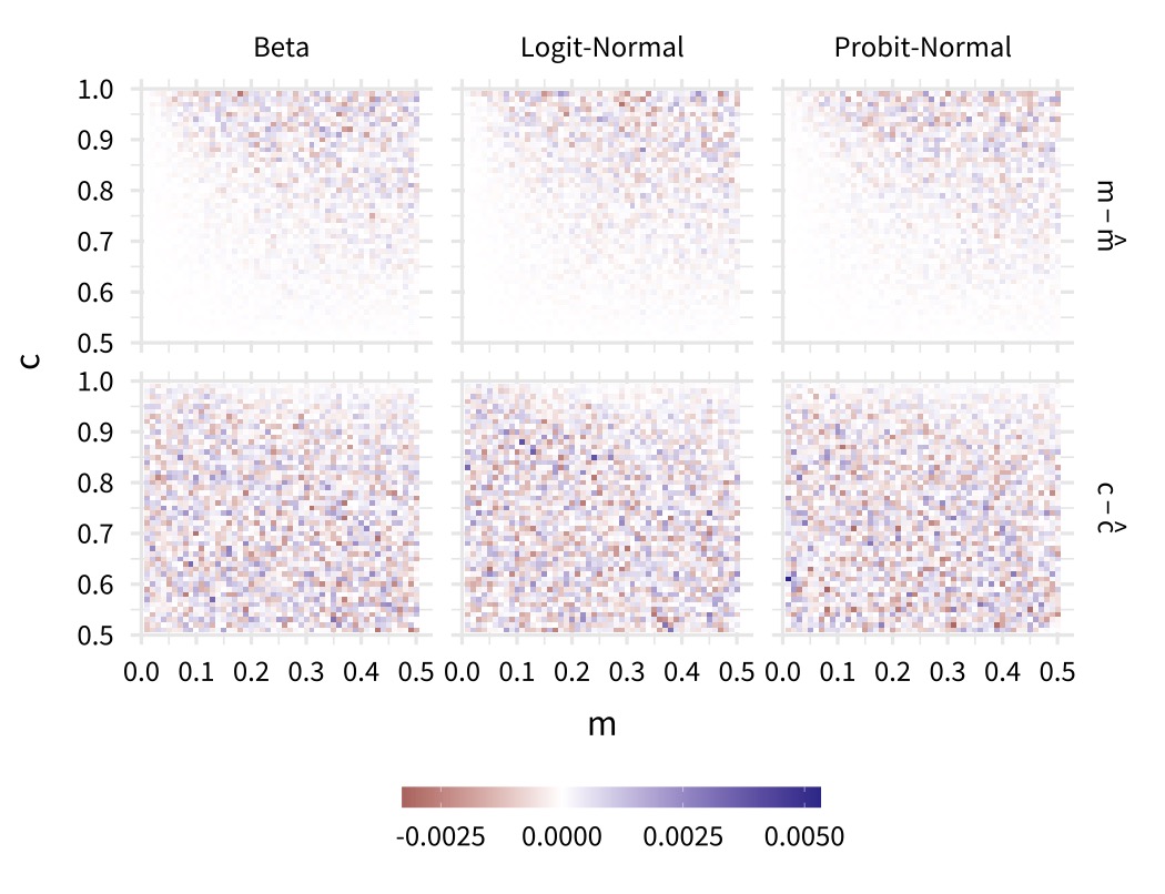
We conducted brief simulation studies to determine the numerical accuracy of our algorithms in recovering the two parameters of the beta, logit-normal, and probit-normal distributions. Our approach involved identifying the parameters of the distribution for a given {,} value, empirically estimating the {,} of this distribution via randomly drawing a large number of risks and response values, and comparing these estimates with the original values.
We performed this simulation for each combination of and . Note that was capped at 0.5 because for all three distributions, the solutions for {, } and {, } are mirror images of each other around (for the beta distribution, the two solutions have their and interchanged, and for the other two, the s are negative of each other). As such the solution for can be derived from the corresponding solution for .
For each {,} value, the size of the simulated data was based on targeting standard error (SE) of 0.001 around both metrics. This value was chosen so that at least the two digits after the decimal points remain significant. For we used the Wald-type SE formula to determine the required sample size. For , we used the SE formula by Newcombe10. The target sample size was the maximum of the two values. We calculated the differences between {,} and {, }.
Simulation results are shown in Figure 1, and illustrate that our algorithm could recover the parameters successfully for typical {,} values, with error not exceeding 0.005.
Remarks
In this work, we showed that a family of strictly continuous distributions with support on [0,1] can be identified by knowing their expected value and c-statistic. The regularity condition that we impose was ‘quantile identifiability’: that knowing two quantiles of the distribution is sufficient for characterizing them. The general two-parameter family of distributions that are often used to model probabilities, including beta, logit-normal, and probit-normal, satisfy this condition. To test the numerical accuracy of our proposed algorithm for mapping mean and c-statistic to the parameters of two-parameter distributions, we performed brief simulation studies. The mapping algorithm is developed into the publicly available mcmapper R package.
In our simulation study, we showed satisfactory performance for a plausible range of mean and c-statistic. However, these algorithms might struggle at extreme ranges, especially for the c-statistic (e.g., for or ). This is because the CDF can be very flat (within the floating point precision of the computing device) in extended parts of its range in such cases, making numerical integration inaccurate. As well, the surface of the function mapping to the parameters of the distribution might be flat around the solution in such extreme cases, causing the gradient descent algorithm to fail to converge. In general, extreme values of the c-statistic are not plausible in real-world situations. A c-statistic that is very close to 1, for example, might indicate a complete separation of cases and controls. Reciprocally, a c-statistic that is very close to 0.5 signals no variability in risks. In such situations, the appropriateness of modeling the risk as a continuous distribution might be doubtful.
In pursuing this development we were motivated by several recent developments in risk prediction modeling that require specifying the distribution of predicted risks in a population, in particular sample size calculations and Value of Information analyses3,5. The report on the development of a risk prediction model often contains an estimate of the expected value of risk and the c-statistic of the model for predicting . Assuming that the model is moderately calibrated in the development population (i.e., ), the identifiability results in this work can directly be applied to recover the parameters of the distribution. In applying these developments, the onus is on the investigator to decide on the appropriateness of the family of distributions. Sometimes there is auxiliary information in a report, such as the shape of the receiver operating characteristic curve or the histogram of predicted risks, that the investigator can draw on (e.g., which family of distributions generates the best matching histogram once the parameters are recovered?), and perform sensitivity analyses as required.
Do these developments apply with other measures of centrality such as median and mode? This is obvious for some specific cases. For example, for both the logit-normal and probit-normal distributions, knowing the median directly identifies ; and is then uniquely determined by . As well, the mode of the beta distribution establishes a linear relation between its parameters, so one can express one parameter in terms of the other given the mode, and solve for the remaining parameter by knowing . However, in the Appendix, we provide counterexamples that show that under the regularity conditions stated here, the lemma is not generally applicable with the median or mode.
References
References
-
1.
Steyerberg EW, Vergouwe Y. Towards better clinical prediction models: Seven steps for development and an ABCD for validation. European Heart Journal 2014; 35: 1925–1931.
-
2.
Vickers AJ, Elkin EB. Decision curve analysis: A novel method for evaluating prediction models. 2006; 26: 565–574.
-
3.
Riley RD, Debray TPA, Collins GS, et al. Minimum sample size for external validation of a clinical prediction model with a binary outcome. Stat Med 2021; 40: 4230–4251.
-
4.
Pavlou M, Qu C, Omar RZ, et al. Estimation of required sample size for external validation of risk models for binary outcomes. Stat Methods Med Res 2021; 30: 2187–2206.
-
5.
Sadatsafavi M, Lee TY, Wynants L, et al. Value-of-Information Analysis for External Validation of Risk Prediction Models. Medical Decision Making: An International Journal of the Society for Medical Decision Making 2023; 43: 564–575.
-
6.
Riley RD, Snell KIE, Archer L, et al. Evaluation of clinical prediction models (part 3): Calculating the sample size required for an external validation study. BMJ 2024; 384: e074821.
-
7.
Shih N. The model identification of beta distribution based on quantiles. Journal of Statistical Computation and Simulation 2015; 85: 2022–2032.
-
8.
Sadatsafavi M. The mcmapper R package (development version), https://github.com/resplab/mcmapper (accessed 15 August 2024).
-
9.
Holmes JB, Schofield MR. Moments of the logit-normal distribution. Communications in Statistics - Theory and Methods 2022; 51: 610–623.
-
10.
Newcombe RG. Confidence intervals for an effect size measure based on the Mann-Whitney statistic. Part 2: Asymptotic methods and evaluation. Stat Med 2006; 25: 559–573.
Appendix
To generate counterexamples, we employ the fact that for any distribution with support on [0,1], the distribution whose PDF is the mirror image of , corresponding to transformation, has the same c-statistic as (as one can change the label of cases and controls and arrive at the original distribution). Our counterexamples involve defining the family of distributions based on the mixture of triangular distributions whose mirror image is also the member of the same family. To proceed, define a triangular distribution by (, , ), where is the lower bound, is the upper bound, and is the mode of the distribution. For the case of mode, consider the family of distributions indexed by a single parameter , constructed by a mixture of two triangular distributions such that 3/4 of the mass is from the triangular distribution and 1/4 is from . This family of distributions satisfies the regularity conditions. Direct evaluation of the PDF of this familty of distributions reveals that the mode is always at . A mirror image of any member of this distribution corresponds to another distribution within the same family with transformation. But the mirror distribution has the same (as explained above) and the same mode (at ), violating the identifiability claim. A similar counterexample can be constructed for the median: construct a family of distributions indexed by which is based on an equal mixture of the two triangular distributions and . This family satisfies the regularity conditions, with all members having the same median at . But again, the transformation generates another, distinct member from the same family (corresponding to transformation), with the same median and .