Negative Charge Transfer Energy in Correlated Compounds

Abstract

In correlated compounds containing cations in high formal oxidation states (assigned by assuming that anions attain full valence shells), the energy of ligand to cation charge transfer can become small or even negative. This yields compounds with a high degree of covalence and can lead to a self-doping of holes into the ligand states of the valence band. Such compounds are of particular topical interest, as highly studied perovskite oxides containing trivalent nickel or tetravalent iron are negative charge transfer systems, as are nickel-containing lithium ion battery cathode materials. In this report, we review the topic of negative charge transfer energy, with an emphasis on plots and diagrams as analysis tools, in the spirit of the celebrated Tanabe-Sugano diagrams which are the focus of this Special Topics Issue.

I Introduction

Seven decades ago, Tanabe and Sugano introduced their diagrams as a transformative concept in materials science [1, 2] . Tanabe-Sugano diagrams provide an excellent visualization and analysis tool for the multi-electron states in correlated compounds. Particularly illuminating are phenomena such as spin state transitions, which appear in the diagrams as level crossings resulting from the competition between crystal and ligand fields as well as Coulomb and exchange interactions.

While Tanabe-Sugano diagrams are incredibly useful in relatively ionic compounds, when covalence becomes strong it may become important to consider hybridization effects directly, rather than the typical indirect approach via effective ligand field splittings and reductions in atomic Coulomb and exchange interactions. Strong covalence can originate from large hopping integrals (i.e. valence orbital overlap of cations and ligands), but can also originate from small or negative charge transfer energies and can subsequently result in a breakdown of perturbative approaches. Here, charge transfer energy is defined as the energy required to transfer a ligand valence electron (e.g. oxygen $2p$ electron) to a cation valence shell (e.g. transition metal $d$ shell). In this work, we explore the field of negative charge transfer energy compounds in a similar spirit to Tanabe-Sugano diagrams, where plots of particular parameter series can provide crucial insight into the energetics and correlated states of such materials.

II Charge Transfer Energetics

A suitable starting point to introduce charge transfer energetics is the single impurity Anderson model (SIAM) [3], consisting of a single correlated impurity coupled to a non-interacting bath. While early studies of charge transfer energetics often used cluster models [4, 5], by including the ligand bandwidth one can more clearly distinguish between different charge transfer classes. For the SIAM, assuming an impurity with a valence $d$ shell, we have a Hamiltonian

$$H=H_{I}+H_{B}+H_{V}$$ (1)

which consists of terms for the impurity $H_{I}$, the bath $H_{B}$, and their hybridization interaction $H_{V}$. The impurity term includes the onsite energies of the $d$ shell and the local Coulomb interaction,

$$H_{I}=\sum_{\tau}\epsilon_{d,\tau}\bm{d}^{{\dagger}}_{\tau}\bm{d}^{\phantom{{\dagger}}}_{\tau}+\sum_{\tau_{1},\tau_{2},\tau_{3},\tau_{4}}U_{\tau_{1},\tau_{2},\tau_{3},\tau_{4}}\bm{d}^{{\dagger}}_{\tau_{1}}\bm{d}^{{\dagger}}_{\tau_{2}}\bm{d}^{\phantom{{\dagger}}}_{\tau_{3}}\bm{d}^{\phantom{{\dagger}}}_{\tau_{4}},$$ (2)

with $\tau$ labeling the 10 different $3d$ spin-orbitals and $\bm{d}^{{\dagger}}_{\tau}$ ($\bm{d}^{\phantom{{\dagger}}}_{\tau}$) the operator creating (annihilating) an electron in orbital $\tau$. The first term gives the onsite energy and the second gives the Coulomb interaction. Depending on the local point group symmetry, energy $\epsilon_{d,\tau}$ may include crystal field splitting, which for example in $O_{h}$ point group symmetry would give different onsite energies for the $e_{g}$ orbitals ($3z^{2}-r^{2}$, and $x^{2}-y^{2}$) than for the $t_{2g}$ orbitals ($yz$, $xz$, and $xy$). The Coulomb interaction can contain the typical monopole term (Racah $A$ parameter or Slater $F^{0}$) as well as higher order multipoles (Racah $B$ and $C$ parameters or Slater $F^{2}$ and $F^{4}$) which lead to atomic multiplet splitting.

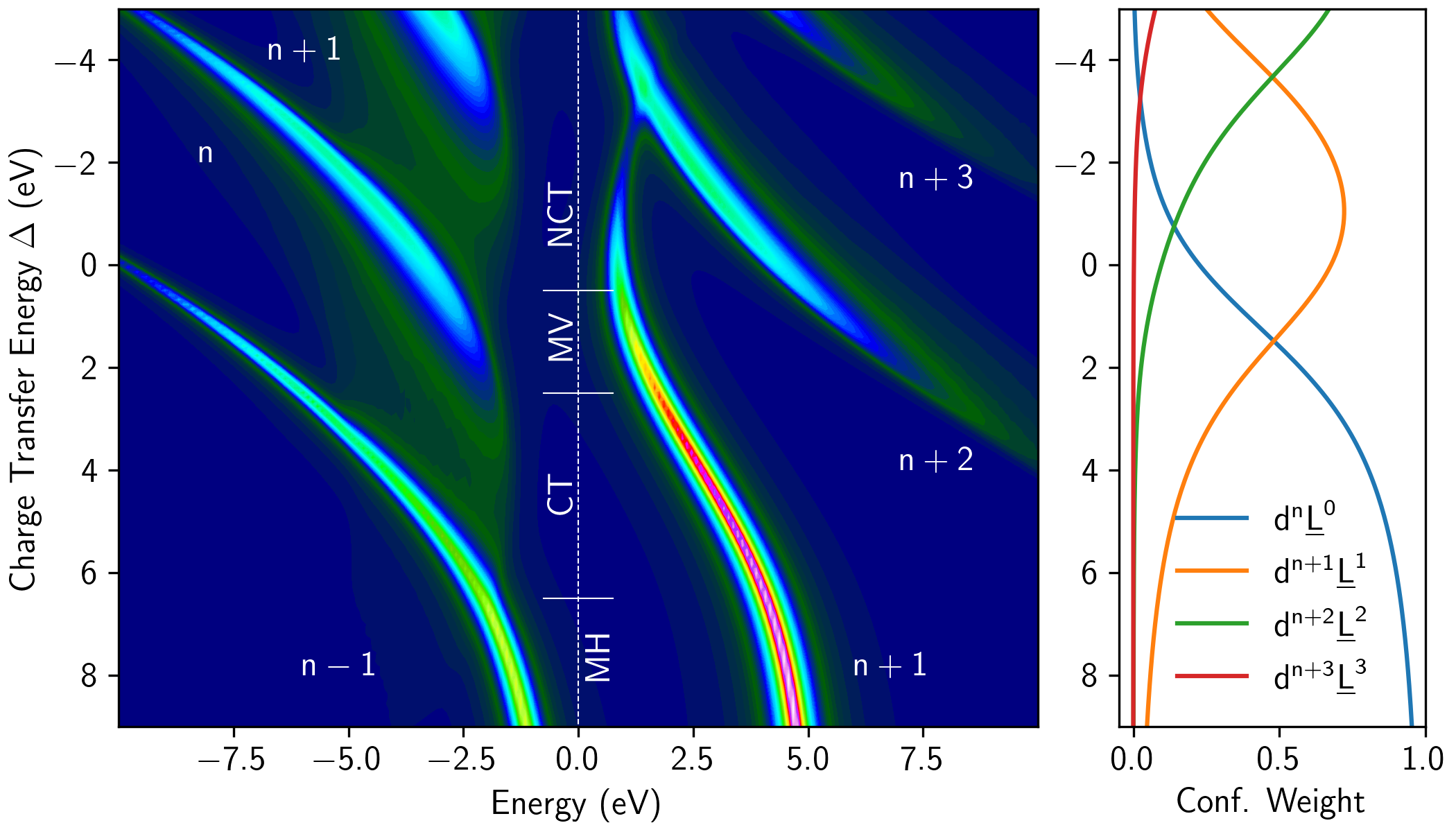
Figure 1: (Color online) (Left) Electron removal and addition spectra for the Anderson impurity model at different charge transfer energies. Addition and removal features are labelled according to the corresponding impurity electron counts, assuming a formal impurity occupation of $d^{n}$. Four regions are identified for specific charge transfer energy ranges: Mott-Hubbard (MH), positive charge transfer (CT), mixed-valence (MV), and negative charge transfer (NCT). (Right) Configuration weights in the ground state wavefunction over the same range of charge transfer energies.

The bath term of the Hamiltonian can be defined in various ways. In a conventional Anderson geometry [3], the impurity couples to all bath sites independently, and there is no coupling between bath sites. Alternatively, an equivalent model can be constructed in what might be called a Wilson geometry [6], where the impurity couples to one bath site, and all bath sites are coupled in a chain extending from this first site [7]. In this geometry, the first bath site can correspond to nearest neighbours, and subsequent bath sites represent linear combinations of the shells from successively further neighbouring atoms. In this Wilson geometry we have for the bath

$$H_{B}= \sum_{k=1}^{N_{L}}\sum_{\tau}\epsilon_{L,k,\tau}\cdot\left(\mathbf{L}^{\dagger}_{k,\tau}\mathbf{L}_{k,\tau}\right)$$ (3)

$$+\frac{W}{4}\sum_{k=1}^{N_{L}-1}\sum_{\tau}\left(\mathbf{L}^{\dagger}_{k,\tau}\mathbf{L}_{k+1,\tau}+\mathbf{L}^{\dagger}_{k+1,\tau}\mathbf{L}_{k,\tau}\right)$$

which enumerates, over $k$, a set of $N_{L}$ ligand shells with creation (annihilation) operator $\mathbf{L^{\dagger}}_{k,\tau}$ ($\mathbf{L}_{k,\tau}$) at energy $\epsilon_{L,k,\tau}$ with a combined spin and orbital index $\tau$. The second term gives the hybridization of the chain of ligand atoms, yielding a band of finite width $W$. Note that for this bath we neglect all Coulomb and exchange interactions involving the bath atoms, assuming that they can be approximated by a one electron band structure which includes these interactions in a mean field average and exchange correlation fashion. This bath is coupled to the impurity via

$$H_{V}=\sum_{\tau}V_{\tau}\left(\mathbf{d}^{\dagger}_{\tau}\mathbf{L}_{1,\tau}+\mathbf{L}^{\dagger}_{1,\tau}\mathbf{d}_{\tau}\right)$$ (4)

where $V_{\tau}$ is the hopping integral from spin orbital $\tau$ of the impurity to first bath site (i.e. the nearest neighbours).

Note that this SIAM Hamiltonian easily reduces to the popular local cluster model when we truncate the bath at the first site. Such single cluster models, typically referred to as multiplet ligand field theory (MLFT) [8] or charge transfer multiplet (CTM) models [9], have been very successful in studying the electronic structure and core level spectroscopy of correlated compounds. Early applications of the cluster model for $3d$ oxides included studies of NiO [4, 5] and CuO [10].

The onsite energies of the impurity and ligands can be defined in terms of charge transfer energy $\Delta$ and Coulomb interaction energy $U$, which can be more readily related to experiments (in particular core level spectroscopy). For an impurity with a formal number of $n$ electrons (e.g. $n=8$ for a Ni²⁺ compound), we can define a reference energy for the $d^{n}$ configuration,

$$n\epsilon_{d}+10N_{L}\epsilon_{L}+n\left(n-1\right)U/2=0$$ (5)

and assign charge transfer energy $\Delta$ to the excited configuration where a ligand electron has transferred to the $d$ shell,

$$\left(n+1\right)\epsilon_{d}+\left(10N_{L}-1\right)\epsilon_{L}+n\left(n+1\right)U/2=\Delta$$ (6)

We can solve these equations for $\epsilon_{d}$ and $\epsilon_{L}$ to recast our Hamiltonian into these more common parameters of $U$ and $\Delta$. The Hamiltonian is then typically solved using a configuration interaction approach, expanding the wavefunction by configurations of the form $|d^{n+m}\underline{L}^{m}\rangle$, where $\underline{L}^{m}$ denotes a configuration with $m$ ligand holes. Using this approach Zaanen, Sawatzky, and Allen developed a classification of Mott-Hubbard (MH) and charge transfer (CT) insulators [11]. While in the former, the lowest energy charge fluctuations are governed by the Coulomb interaction energy $U$ and are of the form

$$2d^{n}\rightarrow d^{n-1}+d^{n+1}$$ (7)

in the latter the fluctuations are governed by the charge transfer energy $\Delta$ and are of the type

$$d^{n}\rightarrow d^{n+1}\underline{L}$$ (8)

This distinction between different types of compounds can be clearly demonstrated via plots of the impurity one electron removal and addition spectra. In Fig. 1 we plot on the left these electron addition and removal spectra for the SIAM as a function of charge transfer energy. The SIAM was implemented and solved using the software QUANTY [12, 7, 13]. For large charge transfer energies, one clearly sees the upper and lower Mott-Hubbard bands (though not strictly bands in the impurity model) which define the conductivity gap. This gap is roughly equivalent to $U$, and is verification of the ideas of Mott [14, 15], originally provided to explain the unexpected insulating nature of some transition metal compounds observed by de Boer and Verwey [16]. These ideas of Mott were later formalized by Hubbard [17, 18]. In the diagram of Fig. 1, we label the features according to the number of electrons – in this Mott-Hubbard regime with large charge transfer energies, the ground state is primarily $|d^{n}\rangle$, so the removal and addition peaks have $n-1$ and $n+1$ electrons, respectively. The ground state character is shown in the right plot of Fig. 1, where the wavefunction is decomposed into different configurations and their weight is plotted for the same values of $\Delta$.

For smaller charge transfer energies, we enter the charge transfer (CT) insulator regime, where now the lowest energy electron removal states (shown by the broad, weak, band-like feature at small removal energies near $\Delta=4\leavevmode\nobreak\ \mathrm{eV}$) are of $d^{n}\underline{L}$ character. In the right panel for this charge transfer energy, one sees the configurations of the type $d^{n+1}\underline{L}^{1}$ gain more weight in the ground state.

Continuing to smaller charge transfer energies, we enter the mixed-valence (M-V) regime, where the ground state is compose of near-equal weights of $d^{n}$ and $d^{n+1}\underline{L}$. Correspondingly one has two strong electron removal configurations ($d^{n-1}$ and $d^{n}\underline{L}$) and two strong electron addition configurations ($d^{n+1}$ and $d^{n+2}\underline{L}$). A clear example of such a compound is SmB₆, where the electron removal features are observed in photoemission spectra [19]. In this case, the weak hybridization interaction facilitates a clear distinction between the two valences present, and in particular there is a clear separation of valences in momentum space. While some transition metal oxides have charge transfer energies that would place them in the mixed valence regime, their hybridization strengths are stronger, leading to a much more covalent wavefunction and not as clear separation of valences.

Finally, moving to even smaller charge transfer energies, we enter the negative charge transfer regime, where the ground state is dominated by the $d^{n+1}\underline{L}$ configuration (Fig. 1, right panel). Here, the removal spectra are primarily of nature $d^{n}\underline{L}$ and addition spectra of type $d^{n+1}$ and $d^{n+2}\underline{L}$. The strong ligand hole component in the ground state indicates a self-doping [20] of the ligand band. In examples such as the perovskite rare earth nickelates (e.g. NdNiO₃) and alkaline earth ferrates (e.g. SrFeO₃), this self-doping corresponds abundent oxygen holes in the ground state configuration, which have been verified by various spectroscopies [21, 22].

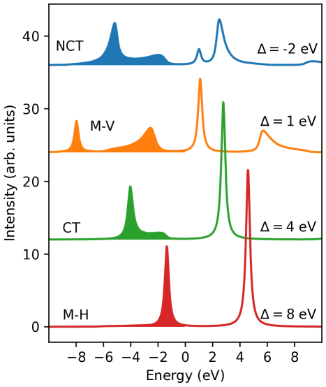
Figure 2: (Color online) Selected electron removal (filled) and addition (unfilled) spectra extracted from Fig. 1. The specific charge transfer energies are indicated, as are the corresponding classification of compounds. A Coulomb interaction energy of $U=5\leavevmode\nobreak\ \mathrm{eV}$ was used for the computation.

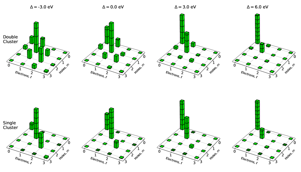
Figure 3: (Color online) Comparison of the ground state wavefunctions obtained in the single cluster ligand field theory and double cluster models for various charge transfer energies. The bars show the weight of the $|d^{n+\ell}\underline{L}^{m}\rangle$ configurations. Scale markings on bars occur in intervals of 0.1, and the wavefunctions are normalized to a total weight of 1.

In Fig. 2, we extract line cuts of the electron addition and removal spectra for charge transfer energies indicative of these four classes of compounds. Here, the upper and lower Mott-Hubbard states are evident, separated by $\scriptstyle\mathtt{\sim}$5 eV, which was the value of $U$ used in the SIAM calculation. In the case of the charge transfer (CT) insulator, the ligand band is more clearly seen in the electron removal spectrum, demonstrating the the lowest energy removal states are of ligand character. Again the four characteristic features are seen in the mixed valence spectrum, and the broad, strongly hybridized ligand states are evident in the negative charge transfer (NCT) case.

As shown above, the SIAM is a useful tool for demonstrating these four classes of compounds. However, an impurity model cannot appropriately model self-doping and intersite cation fluctuations, as a single atom coupled to a continuum bath cannot affect the filling of the bath. To capture self-doping, and the nonlocal fluctuations introduced in such a case, one needs a more sophisticated method like dynamical mean field theory (DMFT). A computationally simpler alternative, particularly applicable to perovskite type of oxides, is the double cluster model [22]. Here, one constructs two ligand field theory clusters which include a cation and nearest neighbour ligands, and then couples them together via symmetry-appropriate hybridization operators. The effect is a system with appropriate metal concentration, which can then lead to significant self-doping of ligands and subsequent intersite fluctuations.

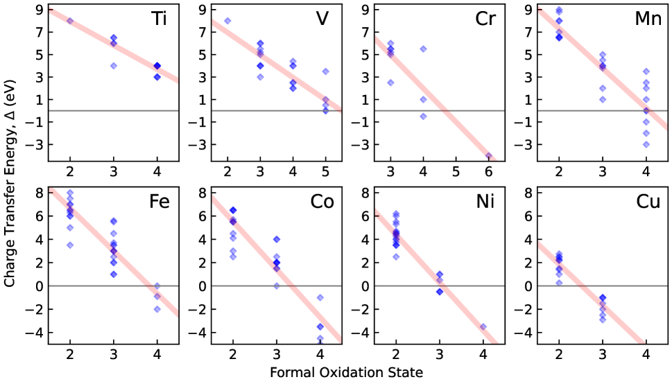
Figure 4: (Color online) Charge transfer energies of $3d$ transition metal oxides compiled from published studies. The data points are plotted with transparency so that overlapping points are evident via higher opacity. Tables with references for all compounds can be found in the Appendix.

In Fig. 3, we compare ground state wavefunction decompositions for a single cluster (i.e. the SIAM with only nearest neighbours and thus zero ligand bandwidth) and the double cluster model, for values of charge transfer energy $\Delta$ spanning from the Mott-Hubbard to negative charge transfer regimes. Specifically, for the single cluster, we take the Hamiltonian from Eq. 1, but limit the bath term from Eq. 3 to $k=1$ (nearest neighbours). The result is a single cluster Hamiltonian, $H_{SC}$. For the double cluster model, we use two single cluster Hamiltonians, labelled $A$ and $B$, and introduce hybridization between them,

$$H_{DC}=H_{SC,A}+H_{SC,B}+H_{mix}$$ (9)

where the hybridization operator has the form

$$H_{mix}=\sqrt{x}\sum_{\tau}V_{\tau} \left(\mathbf{d_{A}}^{\dagger}_{\tau}\mathbf{L_{B}}_{\tau}+\mathbf{L_{B}}^{\dagger}_{\tau}\mathbf{d_{A}}_{\tau}\right.$$ (10)

$$\left.+\mathbf{d_{B}}^{\dagger}_{\tau}\mathbf{L_{A}}_{\tau}+\mathbf{L_{A}}^{\dagger}_{\tau}\mathbf{d_{B}}_{\tau}\right)$$

and the original hybridization operator of Eq. 4 is correspondingly scaled by $\sqrt{1-x}$. In this formulation, the parameter $x$ scales the coupling between clusters. In perovskite oxides, a value of $\scriptstyle\mathtt{\sim}$0.3 is used, which agrees well with the crystal structure symmetry [22]. This value is used in Fig. 3, where the double cluster ground states are compared to those of a single cluster. In the single cluster regime, beginning with a full ligand shell and a formal (stoichiometry defined) $d$ shell filling of $d^{n}$, one is restricted to configurations of the form $|d^{n+m}\underline{L}^{m}\rangle$ in the ground state wavefunction. However, for the double cluster model, intersite fluctuations introduce more general configurations of the form $|d^{n+\ell}\underline{L}^{m}\rangle$.

For relatively large charge transfer energies in the Mott-Hubbard or positive charge transfer regimes (e.g. $\Delta$ of 3.0 or 6.0 eV in Fig. 3), the two models exhibit similar wavefunctions. The full ligand shell suppresses nonlocal charge fluctuations, and the configurations are primarily restricted to the $|d^{n+m}\underline{L}^{m}\rangle$ type, forming the diagonals of the plots in the figure. However, for smaller charge transfer energies ($\Delta$ of 0.0 or -3.0 eV in Fig. 3), the self-doping of significant ligand holes leads to more pronounced nonlocal charge flucutations, and the wavefunction weight spreads away from this diagonal to include significant character of the $|d^{n+\ell}\underline{L}^{m}\rangle$ type. It was shown that these intersite charge fluctuations are important for the perovskite nickelates [22, 23, 24].

III Trends in Charge Transfer Energy and Examples of Negative Charge Transfer Materials

The charge transfer energy is determined by the cation electron affinity and the anion electronegativity. Accordingly, compounds with small or negative charge transfer energy tend to contain cations from later in the transition element series with high formal oxidation states, and/or with heavier anions. Several previous works have investigated trends in the charge transfer energies of various compounds, which verified these general expectations [25, 26, 27]. It is now roughly three decades since these illuminating works, so in Figure 4 we compile charge transfer energies collected for $3d$ oxides from an extensive literature search up to the present day. We plot these charge transfer energies against formal oxidation state for oxides of the eight transition metals spanning from Ti to Cu. In each case we also plot in red a linear regression to the collected data to better visualize the trends in the charge transfer energy. The data and references for this plot are given in the tables of the Appendix.

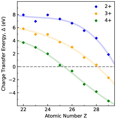
Figure 5: (Color online) Trends of charge transfer energy $\Delta$ versus atomic number for several different formal oxidation states. The values plotted are extracted from the linear regressions to the data of Fig. 4. The lines are a third order polynomial fit to aid in visualizing the trends.

While there is some scatter in the data (see the Appendix for further discussion), it is clear from Fig. 4 that charge transfer energy decreases roughly linearly with formal oxidation state and generally decreases along the $3d$ series. From the linear regressions of Fig. 4, we extract an average charge transfer energy for common formal oxidation states of the $3d$ series, and plot these in Fig. 5. Here a clear trend is present of decreasing charge transfer energy for higher atomic number in the series as demonstrated in previous works [25, 26, 27]. We see that for oxides, negative charge transfer energies are generally present for tetravalent Fe-Cu ions or trivalent Ni and Cu ions. Apparent from Fig. 4 is that Cr and V negative charge transfer oxides are also possible. For anions with higher electronegativities (sulfur for example) these series are expected to shift downward so that 3+ or even 2+ ions late in the series will be negative charge transfer compounds. We note that in Fig. 5, anomalies for V and Cr may be due to a lack of data for these elements and that the data in Fig. 4 for these elements spans more oxidation states than for other elements and therefore a linear regression may not be appropriate.

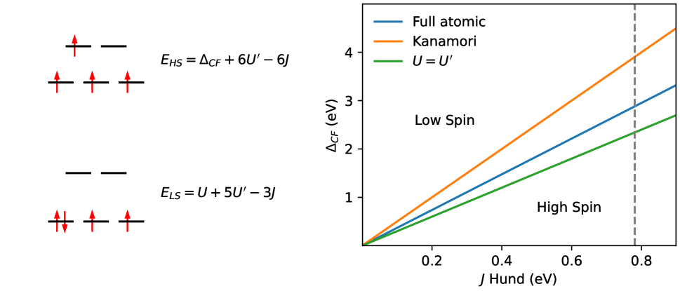
Figure 6: (Color online) (Left) The energetics of high spin and low spin $3d^{4}$ configurations, as determined with the Kanamori approach. (Right) Comparison of the spin state crossover for the full atomic multiplet theory and the Kanamori approach, along with the simplified Kanamori approach with $U^{\prime}=U$. The dashed grey line denotes the free ion value of $J$.

The first report of a solid state compound with negative charge transfer energy was that of NaCuO₂, studied by Mizokawa et al [28]. In this compound, the stoichiometry imposes a high 3+ oxidation state for the Cu, but a negative charge transfer energy yields a ground state that is primarily $d^{9}\underline{L}$. The material is insulating, but the authors determined that the gap is a $p-p$ type gap and therefore NaCuO₂ is neither a Mott-Hubbard or charge-transfer insulator. Follow up studies further clarified the nature of the $d^{9}\underline{L}$ ground state [29, 30, 31].

More recently, the perovskite nickelates $R$NiO₃ (with $R$ a rare earth ion) have been extensively studied. With trivalent rare earths, formal oxidation state rules imply the presence of Ni³⁺, or a $3d^{7}$ configuration. However, due to a negative charge transfer energy, the ground state is primarily $3d^{8}\underline{L}$. Note that the low spin $3d^{7}$ and the $3d^{8}\underline{L}$ are both $S=1/2$ due to the antiferromagnetic coupling of the ligand hole to the Ni. These compounds (except for LaNiO₃) exhibit a metal-insulator transition, with different transition temperatures for compounds having different rare-earth ion [32]. In the insulating phase, the NiO₆ octahedra expand and compress in a breathing distortion following a rocksalt lattice pattern. The compounds also transition into an antiferromagnetic ordered phase with a (1/4,1/4,1/4) ordering vector (in pseudocubic notation).

Early theoretical studies of the perovskite nickelates predicted oxygen- or nickel-based charge ordering depending on the value of charge transfer energy [33]. Later computational studies expressed the ordering in terms of a bond disproportionation [34, 35, 22], where the negative charge transfer $d^{8}\underline{L}$ state disproportionates into $d^{8}\underline{L}^{0}$ and $d^{8}\underline{L}^{2}$. Experimental studies using core level spectroscopy verified the negative charge transfer nature of these compounds [21]. As nickelates can be grown epitaxially in thin film form, and the perovskite structure affords many different substrates which impose geometric and strain effects, numerous studies were carried out on nickelate heterostructures in recent years [36]. Examples include control of emergent properties via tensile and compressive strain [37, 38, 39, 40, 41], ultrathin films with control over the magnetic (non)-collinearity [42], variations of the metal-insulator transition temperature for potential device applications [43], and control of the electronic structure and magnetic order via oxygen vacancy electron doping [44] or substitutional hole doping [45].

The alkaline earth ferrates, $A$FeO₃, where Fe is in a high 4+ formal oxidation state, are also negative charge transfer compounds [46, 47, 48, 49, 50]. CaFeO₃ exhibits a breathing distortion and metal-insulator transition similar to the perovskite nickelates [51]. This is also found to coincide with a bond disproportionation, here into sites of the form $d^{5}\underline{L}^{2}$ and $d^{5}\underline{L}^{0}$ [47]. Also similar to the nickelates, both SrFeO₃ and CaFeO₃ exhibit antiferromagnetic ordering with an ordering vector parallel to the pseudocubic (111) direction. However, different from the nickelates, the antiferromagnetic order is in the form of incommensurate helices [52, 53, 54] which can form topological spin textures [55].

We have focused on oxide compounds up to this point, but the disulfide pyrites FeS₂, CoS₂, and NiS₂ are also negative charge transfer compounds. In these compounds, formal oxidation state assignments would suggest valences of 4- for the S₂ and therefore 4+ for the cations. However, it is instead found that the cations are 2+ and there are self-doped sulfur $3p$ holes [56]. Additionally, the sulfur anions form pairs with full bonding and empty antibonding orbitals such that the S₂ molecule has a $2-$ configuration (similar to superoxides like KO₂). While this is indeed formally a negative charge transfer situation, often an effective positive charge transfer energy is defined for the divalent cations, relative to the full sulfur $3p$ valence band. The compounds have diverse and interesting properties–FeS₂ is a diamagnetic semiconductor, CoS₂ is a ferromagnetic metal, and NiS₂ is an antiferromagnetic Mott insulator [57, 58]. Spectroscopy studies revealed the self-doped nature of the compounds [59, 60], and an impurity model with an explicit self-doped conduction band was used to interpret photoemission spectra [60].

IV The Importance of Atomic Physics

Atomic physics, i.e. multipole Coulomb interactions, generally remain very important for negative charge transfer compounds. In full atomic multiplet theory, the strength of the Coulomb interactions among (all pairs of) electrons are defined by either the radial Slater integrals $F^{k}$ (where $k=0,2,4$ for $d$ electrons) or the Racah parameters $A$, $B$, $C$. These interactions are at times approximated–for example the Kanamori approach [61] uses effective parameters $U$, $J$, and $U^{\prime}$, where $U$ is the Coulomb repulsion of electrons in the same orbital, $J$ is the Hunds’ rule exchange, and $U^{\prime}=U-2J$ is the Coulomb interaction of electrons in different orbitals. The work of Tanabe and Sugano [1, 2] considered the full multiplet interactions, so this dedicated Special Issue is a good avenue to demonstrate the importance of these atomic effects. As an illustrative example, the energies of high spin and low spin configurations for a $3d^{4}$ ion with octahedral coordination within the Kanamori approximation are as given in Fig. 6. Equating these two energies gives us the condition of $\Delta_{CF}=5J$ for the spin state crossover. This line is compared to the crossover computed with full crystal field multiplet theory in the right panel of Figure 6, where we find the condition $\Delta_{CF}\approx 3.69J$. Also shown in the Figure is the simplification $U$=$U^{\prime}$ in the Kanamori approach, where the crossover occurs at $\Delta_{CF}=3J$. Therefore we find the full multiplet result is between the two approximations. While the approximations are of course still very useful tools, care must be taken for compounds which are in close proximity to spin state transitions, as the full atomic approach becomes necessary.

V Conclusion

We have reviewed how correlated compounds can be classified into four regimes, based on the relative values of charge transfer energy ($\Delta$) and Coulomb interaction $U$. In addition to the more common Mott-Hubbard ($U<\Delta$) and charge transfer ($U>\Delta$) insulators, for small values of $\Delta$ one enters the mixed valence and then negative charge transfer regimes. The self-doping of the ligand band for these cases leads to new phenomena such as bond disproportionation, where ligand holes bond asymmetrically between sites. Clearly the anion states become very important in these compounds, and this can mean that non-conventional starting points might be necessary when constructing models to understand the electronic and magnetic structures of these compounds.

Appendix A Appendix: Oxide Charge Transfer Energy Data

This Appendix contains tables of charge transfer energies collected from a literature search of $3d$ transition metal oxides. Each table reports values for compounds containing a specific $3d$ cation, ranging from Ti to Cu in Tables A-I, A-II, A-III, A-IV, A-V, A-VI, A-VII and A-VIII. The data from these tables was used to construct the plots in Fig. 4, which show clear trends in the charge transfer energies with different formal valences. It should be noted that generally relatively large uncertainties exist when extracting charge transfer energies using the typical core level spectroscopy approaches like x-ray photoelectron spectroscopy (XPS) and x-ray absorption spectroscopy (XAS). Thus, there is some scatter in the data contained in these tables, even for different experiments on the same compounds. Further, different techniques can probe effectively different charge transfer energies–the value of $\Delta$ obtained by optimizing cluster model parameters against $2p$ XPS data is fundamentally different from that which would be extracted from oxygen x-ray emission and absorption spectra. Both values are valid, but relate to different defitions of $\Delta$. In compiling the data in the following tables, we have primarily focused on cluster-derived values so that they may be directly compared and thus the trends are meaningful. Of the various approaches to extract charge transfer energies, $2p3d$ resonant inelastic x-ray scattering (RIXS) seems to be especially powerful, as one typically sees a clear charge transfer band, separated or slightly overlapping with $dd$ orbital excitations [62, 63, 64, 65, 66, 67, 68, 69]. When analyzed using a SIAM, the charge transfer energy can often be extracted in a direct and precise way.

Table A-I: Collection of charge transfer energies for Ti oxides from literature.

Compound	Valence	$\Delta$ (eV)	Reference
TiO2	4+	4.0	26
TiO2	4+	4.0	70
TiO2	4+	4.0	71
TiO2	4+	4.0	72
TiO2	4+	3.0	62
TiO2	4+	4.0	73
TiO2	4+	3.0	74
TiO2	4+	4.0	75
SrTiO3	4+	4.0	26
SrTiO3	4+	3.0	74
Ti2O3	3+	6.5	76
Ti2O3	3+	6.5	77, 78
LaTiO3	3+	6.0	79
LaTiO3	3+	4.0	80
YTiO3	3+	6.0	26
TiO	2+	8.0	26

Table A-II: Collection of charge transfer energies for V oxides from literature.

Compound	Valence	$\Delta$ (eV)	Reference
V2O5	5+	0.5	26
V2O5	5+	3.5	75
Ba3V2S4O3	5+	1.0	81
NaV2O5	5+	0.0	82
V6O13	5+	0.0	83
VO2	4+	2.0	71
VO2	4+	2.5	84
VO2	4+	2.0	85
VO2	4+	4.4	75
NaV2O5	4+	4.0	82
V6O13(A)	4+	4.0	83
V6O13(B)	4+	2.5	83
LaVO3	3+	4.0	26
LiVO2	3+	4.0	86
V2O3	3+	4.0	26
V2O3	3+	6.0	77, 82
V2O3	3+	5.5	75
V2OPO4	3+	6.0	87
ZnV2O4	3+	5.2	88
CdV2O4	3+	5.0	88
Ba3V2S4O3	3+	3.0	81
V2OPO4	2+	8.0	87

Table A-III: Collection of charge transfer energies for Cr oxides from literature.

Compound	Valence	$\Delta$ (eV)	Reference
PbCrO3	6+	-4.0	89
CrO2	4+	-0.5	90, 91
CrO2	4+	1.0	85
CrO2	4+	5.5	75
LaCrO3	3+	5.2	79
LaCrO3	3+	5.5	92
YCrO3	3+	2.5	93
PbCrO3	3+	5.0	89
Cr2O3	3+	5.5	77
Cr2O3	3+	6.0	75

Table A-IV: Collection of charge transfer energies for Mn oxides from literature.

Compound	Valence	$\Delta$ (eV)	Reference
Bi3Mn4O12(NO3)	4+	1.0	94
La2MnCoO6	4+	-3.0	95
SrMnO3	4+	2.0	25
CaMnO3	4+	3.5	96
LiMn2O4	4+	-1.0	97
Li2MnO3	4+	0.0	98
LaSr3Mn2O4	4+	-2.0	99
TbSrMn2O6	4+	0.0	100
Pr2MnNiO6	4+	2.5	101
LiMn2O4	3+	4.0	97
LaMnO3	3+	4.5	25
CaMnO3	3+	3.8	96
DyMnO3	3+	4.0	102
LaSr3Mn2O4	3+	2.0	99
Mn2O3	3+	5.0	77
TbSrMn2O6	3+	1.0	100
MnO	2+	6.5	25
MnO	2+	7.0	103
MnO	2+	9.0	104
MnO	2+	8.0	105, 106
MnO	2+	6.5	63
MnO	2+	8.8	107
Mn3WO6	2+	8.0	108
MnWO4	2+	6.5	109
SiO2:Mn	2+	6.6	68

Table A-V: Collection of charge transfer energies for Fe oxides from literature.

Compound	Valence	$\Delta$ (eV)	Reference
SrFeO3	4+	0.0	25
CaFeO3	4+	-2.0	50
BaFeO3	4+	-0.9	110
LaFeO3	3+	2.5	25
CoFe2O4	3+	2.0	111
FePO4	3+	5.6	112
Fe2O3	3+	3.5	25
Fe2O3	3+	3.0	113
Fe2O3	3+	4.5	77
Fe2O3	3+	2.0	114
Fe2O3	3+	3.7	115
Fe2O3	3+	5.5	75
Fe3O4(Td)	3+	3.5	116
Fe3O4(Oh)	3+	3.0	116
SmFeO3	3+	3.0	117
CaBaFe4O7	3+	1.0	118
(In,Fe)2O3	3+	1.0	67
Fe3O4	2+	7.0	116
FeO	2+	6.0	25
FeO	2+	6.5	119
FeO	2+	7.0	72
FeO	2+	6.5	104
FeO	2+	6.3	75
(Fe,Mg)O	2+	7.5	120
FeWO4	2+	8.0	121
FePO4	2+	9.7	112
CaBaFe4O7	2+	5.0	118
FeTiO3	2+	3.5	115
(In,Fe)2O3	2+	6.0	67

Table A-VI: Collection of charge transfer energies for Co oxides from literature.

Compound	Valence	$\Delta$ (eV)	Reference
CaCu3Co4O12	4+	-4.5	122
Ba2CoO4	4+	-3.5	123
BaCoO3	4+	-3.5	124
SrCoO3	4+	-5.0	125
NaxCoO2	4+	-1.0	126
Sr2CoO3Cl	3+	2.5	127
LaCoO3	3+	2.0	128
LaCoO3	3+	2.0	129
BiCoO3	3+	0.0	130
LiCoO2	3+	4.0	131
Sr4CoIrO8	3+	2.0	132
NdCaCoO4	3+	2.0	132
Gd2Ba2Co4O10	3+	2.0	133
NaxCoO2	3+	4.0	126
Ca3Co2O6	3+	1.5	134
Co3O4	3+	1.5	135
CoFe2O4	2+	6.5	111
La2MnCoO6	2+	5.5	95
CoWO4	2+	6.5	109
CoV2O6	2+	6.5	136
CoO	2+	6.5	137
CoO	2+	2.5	138
CoO	2+	3.0	64
CoO	2+	4.1	115
CoO	2+	5.7	139
CoO	2+	5.5	131
Co3O4	2+	4.5	135
SiO2:Co	2+	5.5	68

Table A-VII: Collection of charge transfer energies for Ni oxides from literature.

Compound	Valence	$\Delta$ (eV)	Reference
LiNiO2	4+	-3.5	140
NdNiO3	3+	-0.5	22
PrNiO3	3+	1.0	141
LaNiO3	3+	1.0	142
LiNiO2	3+	-0.5	140
LiNiO2	3+	-0.5	143
Nd4LiNiO8	3+	0.5	97
Li2NiMn3O8	2+	6.0	97
Pr2MnNiO6	2+	3.5	101
Lu2BaNiO5	2+	2.5	144
Y2BaNiO5	2+	3.75	144
Pr2NiO4	2+	3.5	144
La2NiO4	2+	4.25	144
NiO	2+	5.5	144
NiO	2+	4.5	145
NiO	2+	4.5	25
NiO	2+	4.6	146
NiO	2+	4.0	4
NiO	2+	3.5	147, 65
NiO	2+	4.4	115
NiO	2+	5.3	139
NiO	2+	6.2	143
(Zn,Ni)O	2+	4.0	66
(Mg,Ni)O	2+	4.7	148

Table A-VIII: Collection of charge transfer energies for Cu oxides from literature.

Compound	Valence	$\Delta$ (eV)	Reference
NaCuO2	3+	-2.0	28
NaCuO2	3+	-1.0	29
NaCuO2	3+	-1.0	30
NaCuO2	3+	-2.5	31
LaCuO3	3+	-1.0	149
LaCuO3	3+	-2.9	150
KCuO2	3+	-1.5	151
CuO	2+	2.2	152
CuO	2+	2.75	153
CuO	2+	1.5	154
CaCu3Ru4O12	2+	2.2	155
Nd2CuO4	2+	2.5	156, 157
La2CuO4	2+	1.0	154
La2CuO4	2+	1.4	30
La2CuO4	2+	2.3	153
Sr2CuO3	2+	2.5	158
Sr2CuO3	2+	0.25	154

References

- Tanabe and Sugano [1954a] Y. Tanabe and S. Sugano, Journal of the Physical Society of Japan 9, 753 (1954a).
- Tanabe and Sugano [1954b] Y. Tanabe and S. Sugano, Journal of the Physical Society of Japan 9, 766 (1954b).
- Anderson [1961] P. W. Anderson, Phys. Rev. 124, 41 (1961).
- Fujimori and Minami [1984] A. Fujimori and F. Minami, Phys. Rev. B 30, 957 (1984).
- Sawatzky and Allen [1984] G. A. Sawatzky and J. W. Allen, Phys. Rev. Lett. 53, 2339 (1984).
- Wilson [1975] K. G. Wilson, Rev. Mod. Phys. 47, 773 (1975).
- Lu et al. [2014] Y. Lu, M. Höppner, O. Gunnarsson, and M. W. Haverkort, Phys. Rev. B 90, 085102 (2014).
- Haverkort et al. [2012] M. W. Haverkort, M. Zwierzycki, and O. K. Andersen, Phys. Rev. B 85, 165113 (2012).
- de Groot et al. [2021] F. M. de Groot, H. Elnaggar, F. Frati, R. pan Wang, M. U. Delgado-Jaime, M. van Veenendaal, J. Fernandez-Rodriguez, M. W. Haverkort, R. J. Green, G. van der Laan, Y. Kvashnin, A. Hariki, H. Ikeno, H. Ramanantoanina, C. Daul, B. Delley, M. Odelius, M. Lundberg, O. Kuhn, S. I. Bokarev, E. Shirley, J. Vinson, K. Gilmore, M. Stener, G. Fronzoni, P. Decleva, P. Kruger, M. Retegan, Y. Joly, C. Vorwerk, C. Draxl, J. Rehr, and A. Tanaka, Journal of Electron Spectroscopy and Related Phenomena 249, 147061 (2021).
- Eskes et al. [1990] H. Eskes, L. H. Tjeng, and G. A. Sawatzky, Phys. Rev. B 41, 288 (1990).
- Zaanen et al. [1985] J. Zaanen, G. A. Sawatzky, and J. W. Allen, Phys. Rev. Lett. 55, 418 (1985).
- [12] M. W. Haverkort, http://www.quanty.org.
- Haverkort et al. [2014] M. W. Haverkort, G. Sangiovanni, P. Hansmann, A. Toschi, Y. Lu, and S. Macke, Europhysics Letters 108, 57004 (2014).
- Mott and Peierls [1937] N. F. Mott and R. Peierls, Proceedings of the Physical Society 49, 72 (1937).
- Mott [1949] N. F. Mott, Proceedings of the Physical Society. Section A 62, 416 (1949).
- de Boer and Verwey [1937] J. H. de Boer and E. J. W. Verwey, Proceedings of the Physical Society 49, 59 (1937).
- Hubbard [1964a] J. Hubbard, Proceedings of the Royal Society of London. Series A. Mathematical and Physical Sciences 277, 237 (1964a).
- Hubbard [1964b] J. Hubbard, Proceedings of the Royal Society of London. Series A. Mathematical and Physical Sciences 281, 401 (1964b).
- Sawatzky and Green [2016] G. A. Sawatzky and R. J. Green, in Quantum Materials: Experiments and Theory, edited by J. v. d. B. E. Pavarini, E. Koch and G. Sawatzky (Forschungszentrum Julich, 2016).
- Khomskii [1997] D. I. Khomskii, Lithuanian J. Phys. 37, 65 (1997).
- Bisogni et al. [2016] V. Bisogni, S. Catalano, R. J. Green, M. Gibert, R. Scherwitzl, Y. Huang, V. N. Strocov, P. Zubko, S. Balandeh, J.-M. Triscone, G. Sawatzky, and T. Schmitt, Nature Communications 7, 13017 (2016).
- Green et al. [2016] R. J. Green, M. W. Haverkort, and G. A. Sawatzky, Phys. Rev. B 94, 195127 (2016).
- Lu et al. [2018] Y. Lu, D. Betto, K. Fürsich, H. Suzuki, H.-H. Kim, G. Cristiani, G. Logvenov, N. B. Brookes, E. Benckiser, M. W. Haverkort, G. Khaliullin, M. Le Tacon, M. Minola, and B. Keimer, Phys. Rev. X 8, 031014 (2018).
- Fürsich et al. [2019] K. Fürsich, Y. Lu, D. Betto, M. Bluschke, J. Porras, E. Schierle, R. Ortiz, H. Suzuki, G. Cristiani, G. Logvenov, N. B. Brookes, M. W. Haverkort, M. Le Tacon, E. Benckiser, M. Minola, and B. Keimer, Phys. Rev. B 99, 165124 (2019).
- Bocquet et al. [1992a] A. E. Bocquet, T. Mizokawa, T. Saitoh, H. Namatame, and A. Fujimori, Phys. Rev. B 46, 3771 (1992a).
- Bocquet et al. [1996a] A. E. Bocquet, T. Mizokawa, K. Morikawa, A. Fujimori, S. R. Barman, K. Maiti, D. D. Sarma, Y. Tokura, and M. Onoda, Phys. Rev. B 53, 1161 (1996a).
- Fujimori et al. [1993] A. Fujimori, A. Bocquet, T. Saitoh, and T. Mizokawa, Journal of Electron Spectroscopy and Related Phenomena 62, 141 (1993).
- Mizokawa et al. [1991] T. Mizokawa, H. Namatame, A. Fujimori, K. Akeyama, H. Kondoh, H. Kuroda, and N. Kosugi, Phys. Rev. Lett. 67, 1638 (1991).
- Mizokawa et al. [1994] T. Mizokawa, A. Fujimori, H. Namatame, K. Akeyama, and N. Kosugi, Phys. Rev. B 49, 7193 (1994).
- Okada et al. [1991] K. Okada, A. Kotani, B. Thole, and G. Sawatzky, Solid State Communications 77, 835 (1991).
- Nimkar et al. [1993] S. Nimkar, D. D. Sarma, and H. R. Krishnamurthy, Phys. Rev. B 47, 10927 (1993).
- Medarde [1997] M. Medarde, Journal of Physics: Condensed Matter 9, 1679 (1997).
- Mizokawa et al. [2000] T. Mizokawa, D. I. Khomskii, and G. A. Sawatzky, Phys. Rev. B 61, 11263 (2000).
- Lau and Millis [2013] B. Lau and A. J. Millis, Phys. Rev. Lett. 110, 126404 (2013).
- Johnston et al. [2014] S. Johnston, A. Mukherjee, I. Elfimov, M. Berciu, and G. A. Sawatzky, Phys. Rev. Lett. 112, 106404 (2014).
- Catalano et al. [2018] S. Catalano, M. Gibert, J. Fowlie, J. Íñiguez, J.-M. Triscone, and J. Kreisel, Reports on Progress in Physics 81, 046501 (2018).
- Kim et al. [2020] T. H. Kim, T. R. Paudel, R. J. Green, K. Song, H.-S. Lee, S.-Y. Choi, J. Irwin, B. Noesges, L. J. Brillson, M. S. Rzchowski, G. A. Sawatzky, E. Y. Tsymbal, and C. B. Eom, Phys. Rev. B 101, 121105 (2020).
- Benckiser et al. [2011] E. Benckiser, M. W. Haverkort, S. Brueck, E. Goering, S. Macke, A. Frano, X. Yang, O. K. Andersen, G. Cristiani, H.-U. Habermeier, A. V. Boris, I. Zegkinoglou, P. Wochner, H.-J. Kim, V. Hinkov, and B. Keimer, Nature Materials 10, 189 (2011).
- Liu et al. [2013] J. Liu, M. Kargarian, M. Kareev, B. Gray, P. J. Ryan, A. Cruz, N. Tahir, Y.-D. Chuang, J. Guo, J. M. Rondinelli, J. W. Freeland, G. A. Fiete, and J. Chakhalian, Nature Communications 4, 2714 (2013).
- Wu et al. [2013] M. Wu, E. Benckiser, M. W. Haverkort, A. Frano, Y. Lu, U. Nwankwo, S. Brück, P. Audehm, E. Goering, S. Macke, V. Hinkov, P. Wochner, G. Christiani, S. Heinze, G. Logvenov, H.-U. Habermeier, and B. Keimer, Phys. Rev. B 88, 125124 (2013).
- Frano et al. [2013] A. Frano, E. Schierle, M. W. Haverkort, Y. Lu, M. Wu, S. Blanco-Canosa, U. Nwankwo, A. V. Boris, P. Wochner, G. Cristiani, H. U. Habermeier, G. Logvenov, V. Hinkov, E. Benckiser, E. Weschke, and B. Keimer, Phys. Rev. Lett. 111, 106804 (2013).
- Hepting et al. [2018] M. Hepting, R. J. Green, Z. Zhong, M. Bluschke, Y. E. Suyolcu, S. Macke, A. Frano, S. Catalano, M. Gibert, R. Sutarto, F. He, G. Cristiani, G. Logvenov, Y. Wang, P. A. van Aken, P. Hansmann, M. Le Tacon, J. M. Triscone, G. A. Sawatzky, B. Keimer, and E. Benckiser, Nature Physics 14, 1097+ (2018).
- Liao et al. [2018] Z. Liao, N. Gauquelin, R. J. Green, K. Müller-Caspary, I. Lobato, L. Li, S. Van Aert, J. Verbeeck, M. Huijben, M. N. Grisolia, V. Rouco, R. E. Hage, J. E. Villegas, A. Mercy, M. Bibes, P. Ghosez, G. A. Sawatzky, G. Rijnders, and G. Koster, Proceedings of the National Academy of Sciences 115, 9515 (2018).
- Li et al. [2021] J. Li, R. J. Green, Z. Zhang, R. Sutarto, J. T. Sadowski, Z. Zhu, G. Zhang, D. Zhou, Y. Sun, F. He, S. Ramanathan, and R. Comin, Phys. Rev. Lett. 126, 187602 (2021).
- Patel et al. [2022] R. K. Patel, K. Patra, S. K. Ojha, S. Kumar, S. Sarkar, A. Saha, N. Bhattacharya, J. W. Freeland, J.-W. Kim, P. Ryan, Philip J Mahadevan, and S. Middey, Communications Physics 5, 216 (2022).
- Bocquet et al. [1992b] A. E. Bocquet, A. Fujimori, T. Mizokawa, T. Saitoh, H. Namatame, S. Suga, N. Kimizuka, Y. Takeda, and M. Takano, Phys. Rev. B 45, 1561 (1992b).
- Matsuno et al. [2002] J. Matsuno, T. Mizokawa, A. Fujimori, Y. Takeda, S. Kawasaki, and M. Takano, Phys. Rev. B 66, 193103 (2002).
- Abbate et al. [2002a] M. Abbate, G. Zampieri, J. Okamoto, A. Fujimori, S. Kawasaki, and M. Takano, Phys. Rev. B 65, 165120 (2002a).
- Rogge et al. [2018a] P. C. Rogge, R. U. Chandrasena, A. Cammarata, R. J. Green, P. Shafer, B. M. Lefler, A. Huon, A. Arab, E. Arenholz, H. N. Lee, T.-L. Lee, S. Nemšák, J. M. Rondinelli, A. X. Gray, and S. J. May, Phys. Rev. Mater. 2, 015002 (2018a).
- Rogge et al. [2018b] P. C. Rogge, R. J. Green, P. Shafer, G. Fabbris, A. M. Barbour, B. M. Lefler, E. Arenholz, M. P. M. Dean, and S. J. May, Phys. Rev. B 98, 201115 (2018b).
- Kawasaki et al. [1998] S. Kawasaki, M. Takano, R. Kanno, T. Takeda, and A. Fujimori, Journal of the Physical Society of Japan 67, 1529 (1998).
- Takeda et al. [1972] T. Takeda, Y. Yamaguchi, and H. Watanabe, Journal of the Physical Society of Japan 33, 967 (1972).
- Woodward et al. [2000] P. M. Woodward, D. E. Cox, E. Moshopoulou, A. W. Sleight, and S. Morimoto, Phys. Rev. B 62, 844 (2000).
- Rogge et al. [2019] P. C. Rogge, R. J. Green, R. Sutarto, and S. J. May, Phys. Rev. Mater. 3, 084404 (2019).
- Ishiwata et al. [2020] S. Ishiwata, T. Nakajima, J.-H. Kim, D. S. Inosov, N. Kanazawa, J. S. White, J. L. Gavilano, R. Georgii, K. M. Seemann, G. Brandl, P. Manuel, D. D. Khalyavin, S. Seki, Y. Tokunaga, M. Kinoshita, Y. W. Long, Y. Kaneko, Y. Taguchi, T. Arima, B. Keimer, and Y. Tokura, Phys. Rev. B 101, 134406 (2020).
- Folkerts et al. [1987] W. Folkerts, G. A. Sawatzky, C. Haas, R. A. de Groot, and F. U. Hillebrecht, Journal of Physics C: Solid State Physics 20, 4135 (1987).
- Adachi et al. [1969] K. Adachi, K. Sato, and M. Takeda, Journal of the Physical Society of Japan 26, 631 (1969).
- Ogawa [1979] S. Ogawa, Journal of Applied Physics 50, 2308 (1979).
- Fujimori et al. [1996] A. Fujimori, K. Mamiya, T. Mizokawa, T. Miyadai, T. Sekiguchi, H. Takahashi, N. Môri, and S. Suga, Phys. Rev. B 54, 16329 (1996).
- Bocquet et al. [1996b] A. E. Bocquet, K. Mamiya, T. Mizokawa, A. Fujimori, T. Miyadai, H. Takahashi, M. Môri, and S. Suga, Journal of Physics: Condensed Matter 8, 2389 (1996b).
- Kanamori [1963] J. Kanamori, Progress of Theoretical Physics 30, 275 (1963).
- Matsubara et al. [2000] M. Matsubara, T. Uozumi, A. Kotani, Y. Harada, and S. Shin, Journal of the Physical Society of Japan 69, 1558 (2000).
- Ghiringhelli et al. [2006] G. Ghiringhelli, M. Matsubara, C. Dallera, F. Fracassi, A. Tagliaferri, N. B. Brookes, A. Kotani, and L. Braicovich, Phys. Rev. B 73, 035111 (2006).
- Chiuzbăian et al. [2008] S. G. Chiuzbăian, T. Schmitt, M. Matsubara, A. Kotani, G. Ghiringhelli, C. Dallera, A. Tagliaferri, L. Braicovich, V. Scagnoli, N. B. Brookes, U. Staub, and L. Patthey, Phys. Rev. B 78, 245102 (2008).
- Ghiringhelli et al. [2005] G. Ghiringhelli, M. Matsubara, C. Dallera, F. Fracassi, R. Gusmeroli, A. Piazzalunga, A. Tagliaferri, N. B. Brookes, A. Kotani, and L. Braicovich, Journal of Physics: Condensed Matter 17, 5397 (2005).
- Das et al. [2013] S. C. Das, R. J. Green, J. Podder, T. Z. Regier, G. S. Chang, and A. Moewes, The Journal of Physical Chemistry C 117, 12745 (2013).
- Green et al. [2015] R. J. Green, T. Z. Regier, B. Leedahl, J. A. McLeod, X. H. Xu, G. S. Chang, E. Z. Kurmaev, and A. Moewes, Phys. Rev. Lett. 115, 167401 (2015).
- Green et al. [2014] R. J. Green, D. A. Zatsepin, D. J. St. Onge, E. Z. Kurmaev, N. V. Gavrilov, A. F. Zatsepin, and A. Moewes, Journal of Applied Physics 115, 103708 (2014).
- Hariki et al. [2020] A. Hariki, M. Winder, T. Uozumi, and J. Kuneš, Phys. Rev. B 101, 115130 (2020).
- Okada et al. [1994] K. Okada, T. Uozumi, and A. Kotani, Journal of the Physical Society of Japan 63, 3176 (1994).
- Uozumi et al. [1993] T. Uozumi, K. Okada, and A. Kotani, Journal of the Physical Society of Japan 62, 2595 (1993).
- Tanaka and Jo [1994] A. Tanaka and T. Jo, Journal of the Physical Society of Japan 63, 2788 (1994).
- Parlebas et al. [1995] J. Parlebas, M. Khan, T. Uozumi, K. Okada, and A. Kotani, Journal of Electron Spectroscopy and Related Phenomena 71, 117 (1995).
- Hariki et al. [2022] A. Hariki, K. Higashi, T. Yamaguchi, J. Li, C. Kalha, M. Mascheck, S. K. Eriksson, T. Wiell, F. M. F. de Groot, and A. Regoutz, Phys. Rev. B 106, 205138 (2022).
- Zimmermann et al. [1999] R. Zimmermann, P. Steiner, R. Claessen, F. Reinert, S. Hüfner, P. Blaha, and P. Dufek, Journal of Physics: Condensed Matter 11, 1657 (1999).
- Chang et al. [2018] C. F. Chang, T. C. Koethe, Z. Hu, J. Weinen, S. Agrestini, L. Zhao, J. Gegner, H. Ott, G. Panaccione, H. Wu, M. W. Haverkort, H. Roth, A. C. Komarek, F. Offi, G. Monaco, Y.-F. Liao, K.-D. Tsuei, H.-J. Lin, C. T. Chen, A. Tanaka, and L. H. Tjeng, Phys. Rev. X 8, 021004 (2018).
- Uozumi et al. [1997] T. Uozumi, K. Okada, A. Kotani, R. Zimmermann, P. Steiner, S. Hüfner, Y. Tezuka, and S. Shin, Journal of Electron Spectroscopy and Related Phenomena 83, 9 (1997).
- Tezuka et al. [1997] Y. Tezuka, S. Shin, T. Uozumi, and A. Kotani, Journal of the Physical Society of Japan 66, 3153 (1997).
- Saitoh et al. [1995] T. Saitoh, A. E. Bocquet, T. Mizokawa, and A. Fujimori, Phys. Rev. B 52, 7934 (1995).
- Haverkort et al. [2005a] M. W. Haverkort, Z. Hu, A. Tanaka, G. Ghiringhelli, H. Roth, M. Cwik, T. Lorenz, C. Schüßler-Langeheine, S. V. Streltsov, A. S. Mylnikova, V. I. Anisimov, C. de Nadai, N. B. Brookes, H. H. Hsieh, H.-J. Lin, C. T. Chen, T. Mizokawa, Y. Taguchi, Y. Tokura, D. I. Khomskii, and L. H. Tjeng, Phys. Rev. Lett. 94, 056401 (2005a).
- Hopkins et al. [2015] E. J. Hopkins, Y. Prots, U. Burkhardt, Y. Watier, Z. Hu, C.-Y. Kuo, J.-C. Chiang, T.-W. Pi, A. Tanaka, L. H. Tjeng, and M. Valldor, Chemistry – A European Journal 21, 7938 (2015).
- Schmitt et al. [2004a] T. Schmitt, L.-C. Duda, M. Matsubara, A. Augustsson, F. Trif, J.-H. Guo, L. Gridneva, T. Uozumi, A. Kotani, and J. Nordgren, Journal of Alloys and Compounds 362, 143 (2004a), proceedings of the Sixth International School and Symposium on Synchrotron Radiation in Natural Science (ISSRNS).
- Schmitt et al. [2004b] T. Schmitt, L.-C. Duda, M. Matsubara, M. Mattesini, M. Klemm, A. Augustsson, J.-H. Guo, T. Uozumi, S. Horn, R. Ahuja, A. Kotani, and J. Nordgren, Phys. Rev. B 69, 125103 (2004b).
- Haverkort et al. [2005b] M. W. Haverkort, Z. Hu, A. Tanaka, W. Reichelt, S. V. Streltsov, M. A. Korotin, V. I. Anisimov, H. H. Hsieh, H.-J. Lin, C. T. Chen, D. I. Khomskii, and L. H. Tjeng, Phys. Rev. Lett. 95, 196404 (2005b).
- Yamaguchi et al. [2024] T. Yamaguchi, K. Higashi, A. Regoutz, Y. Takahashi, M. Lazemi, Q. Che, F. M. F. de Groot, and A. Hariki, Phys. Rev. B 109, 205143 (2024).
- Pen et al. [1997] H. F. Pen, L. H. Tjeng, E. Pellegrin, F. M. F. de Groot, G. A. Sawatzky, M. A. van Veenendaal, and C. T. Chen, Phys. Rev. B 55, 15500 (1997).
- Murota et al. [2020] K. Murota, E. Pachoud, J. P. Attfield, R. Glaum, R. Sutarto, K. Takubo, D. I. Khomskii, and T. Mizokawa, Phys. Rev. B 101, 245106 (2020).
- Takubo et al. [2006] K. Takubo, J.-Y. Son, T. Mizokawa, H. Ueda, M. Isobe, Y. Matsushita, and Y. Ueda, Phys. Rev. B 74, 155103 (2006).
- Zhao et al. [2023] J. Zhao, S.-C. Haw, X. Wang, L. Cao, H.-J. Lin, C.-T. Chen, C. J. Sahle, A. Tanaka, J.-M. Chen, C. Jin, Z. Hu, and L. H. Tjeng, Phys. Rev. B 107, 024107 (2023).
- Korotin et al. [1998] M. A. Korotin, V. I. Anisimov, D. I. Khomskii, and G. A. Sawatzky, Phys. Rev. Lett. 80, 4305 (1998).
- Huang et al. [2003] D. J. Huang, L. H. Tjeng, J. Chen, C. F. Chang, W. P. Wu, S. C. Chung, A. Tanaka, G. Y. Guo, H.-J. Lin, S. G. Shyu, C. C. Wu, and C. T. Chen, Phys. Rev. B 67, 214419 (2003).
- Maiti and Sarma [1996] K. Maiti and D. D. Sarma, Phys. Rev. B 54, 7816 (1996).
- Pal et al. [2018] B. Pal, X. Liu, F. Wen, M. Kareev, A. T. N’Diaye, P. Shafer, E. Arenholz, and J. Chakhalian, Applied Physics Letters 112, 252901 (2018).
- Wadati et al. [2013] H. Wadati, K. Kato, Y. Wakisaka, T. Sudayama, D. Hawthorn, T. Regier, N. Onishi, M. Azuma, Y. Shimakawa, T. Mizokawa, A. Tanaka, and G. Sawatzky, Solid State Communications 162, 18 (2013).
- Burnus et al. [2008] T. Burnus, Z. Hu, H. H. Hsieh, V. L. J. Joly, P. A. Joy, M. W. Haverkort, H. Wu, A. Tanaka, H.-J. Lin, C. T. Chen, and L. H. Tjeng, Phys. Rev. B 77, 125124 (2008).
- Zampieri et al. [2002] G. Zampieri, M. Abbate, F. Prado, A. Caneiro, and E. Morikawa, Physica B: Condensed Matter 320, 51 (2002), proceedings of the Fifth Latin American Workshop on Magnetism, Magnetic Materials and their Applications.
- Liu et al. [2017] H. Liu, J. Zhou, L. Zhang, Z. Hu, C. Kuo, J. Li, Y. Wang, L. H. Tjeng, T.-W. Pi, A. Tanaka, L. Song, J.-Q. Wang, and S. Zhang, The Journal of Physical Chemistry C 121, 16079 (2017).
- Morita et al. [2023] K. Morita, M. Itoda, E. Hosono, D. Asakura, M. Okubo, Y. Takagi, A. Yasui, N. L. Saini, and T. Mizokawa, Journal of the Physical Society of Japan 92, 014702 (2023).
- Wu et al. [2011] H. Wu, C. F. Chang, O. Schumann, Z. Hu, J. C. Cezar, T. Burnus, N. Hollmann, N. B. Brookes, A. Tanaka, M. Braden, L. H. Tjeng, and D. I. Khomskii, Phys. Rev. B 84, 155126 (2011).
- Nguyen et al. [2021] T. L. Nguyen, J. Rubio-Zuazo, G. R. Castro, F. M. F. de Groot, N. Hariharan, S. Elizabeth, M. Oura, Y. C. Tseng, H. J. Lin, and A. Chainani, Phys. Rev. B 103, 245131 (2021).
- Balasubramanian et al. [2018] P. Balasubramanian, S. R. Joshi, R. Yadav, F. M. F. de Groot, A. K. Singh, A. Ray, M. Gupta, A. Singh, S. Maurya, S. Elizabeth, S. Varma, T. Maitra, and V. Malik, Journal of Physics: Condensed Matter 30, 435603 (2018).
- Chen et al. [2010] J. M. Chen, Z. Hu, H. T. Jeng, Y. Y. Chin, J. M. Lee, S. W. Huang, K. T. Lu, C. K. Chen, S. C. Haw, T. L. Chou, H.-J. Lin, C. C. Shen, R. S. Liu, A. Tanaka, L. H. Tjeng, and C. T. Chen, Phys. Rev. B 81, 201102 (2010).
- Fujimori et al. [1990] A. Fujimori, N. Kimizuka, T. Akahane, T. Chiba, S. Kimura, F. Minami, K. Siratori, M. Taniguchi, S. Ogawa, and S. Suga, Phys. Rev. B 42, 7580 (1990).
- Okada and Kotani [1992a] K. Okada and A. Kotani, Journal of the Physical Society of Japan 61, 4619 (1992a).
- Taguchi et al. [1997] M. Taguchi, T. Uozumi, and A. Kotani, Journal of the Physical Society of Japan 66, 247 (1997).
- Shoji et al. [2003] H. Shoji, M. Taguchi, E. Hirai, T. Iwazumi, A. Kotani, S. Nanao, and Y. Isozumi, Journal of the Physical Society of Japan 72, 1560 (2003).
- van Elp et al. [1991a] J. van Elp, R. H. Potze, H. Eskes, R. Berger, and G. A. Sawatzky, Phys. Rev. B 44, 1530 (1991a).
- Maignan et al. [2020] A. Maignan, W. Peng, A. C. Komarek, C.-Y. Kuo, C.-F. Chang, X. Wang, Z. Hu, C.-T. Chen, A. Tanaka, L. H. Tjeng, O. I. Lebedev, and C. Martin, Chemistry of Materials 32, 5664 (2020).
- Hollmann et al. [2010] N. Hollmann, Z. Hu, T. Willers, L. Bohatý, P. Becker, A. Tanaka, H. H. Hsieh, H.-J. Lin, C. T. Chen, and L. H. Tjeng, Phys. Rev. B 82, 184429 (2010).
- Tsuyama et al. [2015] T. Tsuyama, T. Matsuda, S. Chakraverty, J. Okamoto, E. Ikenaga, A. Tanaka, T. Mizokawa, H. Y. Hwang, Y. Tokura, and H. Wadati, Phys. Rev. B 91, 115101 (2015).
- Wang et al. [2021] X. Wang, Z. Hu, S. Agrestini, J. Herrero-Martín, M. Valvidares, R. Sankar, F.-C. Chou, Y.-H. Chu, A. Tanaka, L. H. Tjeng, and E. Pellegrin, Journal of Magnetism and Magnetic Materials 530, 167940 (2021).
- Asakura et al. [2018] D. Asakura, Y. Nanba, Y. Makinose, H. Matsuda, P.-A. Glans, J. Guo, and E. Hosono, ChemPhysChem 19, 988 (2018).
- Fujimori et al. [1986] A. Fujimori, M. Saeki, N. Kimizuka, M. Taniguchi, and S. Suga, Phys. Rev. B 34, 7318 (1986).
- Ellis et al. [2022] D. S. Ellis, R.-P. Wang, D. Wong, J. K. Cooper, C. Schulz, Y.-D. Chuang, Y. Piekner, D. A. Grave, M. Schleuning, D. Friedrich, F. M. F. de Groot, and A. Rothschild, Phys. Rev. B 105, 075101 (2022).
- Ghiasi et al. [2019] M. Ghiasi, A. Hariki, M. Winder, J. Kuneš, A. Regoutz, T.-L. Lee, Y. Hu, J.-P. Rueff, and F. M. F. de Groot, Phys. Rev. B 100, 075146 (2019).
- Chang et al. [2016] C. F. Chang, Z. Hu, S. Klein, X. H. Liu, R. Sutarto, A. Tanaka, J. C. Cezar, N. B. Brookes, H.-J. Lin, H. H. Hsieh, C. T. Chen, A. D. Rata, and L. H. Tjeng, Phys. Rev. X 6, 041011 (2016).
- Kuo et al. [2014] C.-Y. Kuo, Y. Drees, M. T. Fernández-Díaz, L. Zhao, L. Vasylechko, D. Sheptyakov, A. M. T. Bell, T. W. Pi, H.-J. Lin, M.-K. Wu, E. Pellegrin, S. M. Valvidares, Z. W. Li, P. Adler, A. Todorova, R. Küchler, A. Steppke, L. H. Tjeng, Z. Hu, and A. C. Komarek, Phys. Rev. Lett. 113, 217203 (2014).
- Hollmann et al. [2011] N. Hollmann, M. Valldor, H. Wu, Z. Hu, N. Qureshi, T. Willers, Y.-Y. Chin, J. C. Cezar, A. Tanaka, N. B. Brookes, and L. H. Tjeng, Phys. Rev. B 83, 180405 (2011).
- Fujimori et al. [1987] A. Fujimori, N. Kimizuka, M. Taniguchi, and S. Suga, Phys. Rev. B 36, 6691 (1987).
- Haupricht et al. [2010] T. Haupricht, R. Sutarto, M. W. Haverkort, H. Ott, A. Tanaka, H. H. Hsieh, H.-J. Lin, C. T. Chen, Z. Hu, and L. H. Tjeng, Phys. Rev. B 82, 035120 (2010).
- Altendorf et al. [2023] S. G. Altendorf, D. Takegami, A. Meléndez-Sans, C. F. Chang, M. Yoshimura, K. D. Tsuei, A. Tanaka, M. Schmidt, and L. H. Tjeng, Phys. Rev. B 108, 085119 (2023).
- Chin et al. [2021] Y.-Y. Chin, Z. Hu, Y. Shimakawa, J. Yang, Y. Long, A. Tanaka, L. H. Tjeng, H.-J. Lin, and C.-T. Chen, Phys. Rev. B 103, 115149 (2021).
- Takegami et al. [2023a] D. Takegami, Z. Hu, J. Falke, A. Meléndez-Sans, C.-E. Liu, C.-F. Chang, C.-Y. Kuo, C.-T. Chen, H. Guo, A. Komarek, A. Tanaka, S. Hébert, and L. H. Tjeng, Zeitschrift für anorganische und allgemeine Chemie 649, e202300077 (2023a).
- Chin et al. [2019] Y. Y. Chin, Z. Hu, H.-J. Lin, S. Agrestini, J. Weinen, C. Martin, S. Hébert, A. Maignan, A. Tanaka, J. C. Cezar, N. B. Brookes, Y.-F. Liao, K.-D. Tsuei, C. T. Chen, D. I. Khomskii, and L. H. Tjeng, Phys. Rev. B 100, 205139 (2019).
- Potze et al. [1995] R. H. Potze, G. A. Sawatzky, and M. Abbate, Phys. Rev. B 51, 11501 (1995).
- Lin et al. [2010] H.-J. Lin, Y. Y. Chin, Z. Hu, G. J. Shu, F. C. Chou, H. Ohta, K. Yoshimura, S. Hébert, A. Maignan, A. Tanaka, L. H. Tjeng, and C. T. Chen, Phys. Rev. B 81, 115138 (2010).
- Hu et al. [2004] Z. Hu, H. Wu, M. W. Haverkort, H. H. Hsieh, H. J. Lin, T. Lorenz, J. Baier, A. Reichl, I. Bonn, C. Felser, A. Tanaka, C. T. Chen, and L. H. Tjeng, Phys. Rev. Lett. 92, 207402 (2004).
- Haverkort et al. [2006] M. W. Haverkort, Z. Hu, J. C. Cezar, T. Burnus, H. Hartmann, M. Reuther, C. Zobel, T. Lorenz, A. Tanaka, N. B. Brookes, H. H. Hsieh, H.-J. Lin, C. T. Chen, and L. H. Tjeng, Phys. Rev. Lett. 97, 176405 (2006).
- Takegami et al. [2023b] D. Takegami, A. Tanaka, S. Agrestini, Z. Hu, J. Weinen, M. Rotter, C. Schüßler-Langeheine, T. Willers, T. C. Koethe, T. Lorenz, Y. F. Liao, K. D. Tsuei, H.-J. Lin, C. T. Chen, and L. H. Tjeng, Phys. Rev. X 13, 011037 (2023b).
- Sudayama et al. [2011] T. Sudayama, Y. Wakisaka, T. Mizokawa, H. Wadati, G. A. Sawatzky, D. G. Hawthorn, T. Z. Regier, K. Oka, M. Azuma, and Y. Shimakawa, Phys. Rev. B 83, 235105 (2011).
- van Elp et al. [1991b] J. van Elp, J. L. Wieland, H. Eskes, P. Kuiper, G. A. Sawatzky, F. M. F. de Groot, and T. S. Turner, Phys. Rev. B 44, 6090 (1991b).
- Agrestini et al. [2017] S. Agrestini, C.-Y. Kuo, D. Mikhailova, K. Chen, P. Ohresser, T. W. Pi, H. Guo, A. C. Komarek, A. Tanaka, Z. Hu, and L. H. Tjeng, Phys. Rev. B 95, 245131 (2017).
- Hu et al. [2012] Z. Hu, H. Wu, T. C. Koethe, S. N. Barilo, S. V. Shiryaev, G. L. Bychkov, C. Schüßler-Langeheine, T. Lorenz, A. Tanaka, H. H. Hsieh, H.-J. Lin, C. T. Chen, N. B. Brookes, S. Agrestini, Y.-Y. Chin, M. Rotter, and L. H. Tjeng, New Journal of Physics 14, 123025 (2012).
- Burnus et al. [2006] T. Burnus, Z. Hu, M. W. Haverkort, J. C. Cezar, D. Flahaut, V. Hardy, A. Maignan, N. B. Brookes, A. Tanaka, H. H. Hsieh, H.-J. Lin, C. T. Chen, and L. H. Tjeng, Phys. Rev. B 74, 245111 (2006).
- Wang et al. [2022] R.-P. Wang, M.-J. Huang, A. Hariki, J. Okamoto, H.-Y. Huang, A. Singh, D.-J. Huang, P. Nagel, S. Schuppler, T. Haarman, B. Liu, and F. M. F. de Groot, The Journal of Physical Chemistry C 126, 8752 (2022).
- Hollmann et al. [2014] N. Hollmann, S. Agrestini, Z. Hu, Z. He, M. Schmidt, C.-Y. Kuo, M. Rotter, A. A. Nugroho, V. Sessi, A. Tanaka, N. B. Brookes, and L. H. Tjeng, Phys. Rev. B 89, 201101 (2014).
- Csiszar et al. [2005] S. I. Csiszar, M. W. Haverkort, Z. Hu, A. Tanaka, H. H. Hsieh, H.-J. Lin, C. T. Chen, T. Hibma, and L. H. Tjeng, Phys. Rev. Lett. 95, 187205 (2005).
- Okada and Kotani [1992b] K. Okada and A. Kotani, Journal of the Physical Society of Japan 61, 449 (1992b).
- Parmigiani and Sangaletti [1993] F. Parmigiani and L. Sangaletti, Chemical Physics Letters 213, 613 (1993).
- Huang et al. [2023] H. Huang, Y.-C. Chang, Y.-C. Huang, L. Li, A. C. Komarek, L. H. Tjeng, Y. Orikasa, C.-W. Pao, T.-S. Chan, J.-M. Chen, S.-C. Haw, J. Zhou, Y. Wang, H.-J. Lin, C.-T. Chen, C.-L. Dong, C.-Y. Kuo, J.-Q. Wang, Z. Hu, and L. Zhang, Nature Communications 14, 2112 (2023).
- Mizokawa et al. [1996] T. Mizokawa, A. Fujimori, T. Arima, Y. Tokura, N. Mõri, and J. Akimitsu, Journal of Electron Spectroscopy and Related Phenomena 78, 191 (1996).
- Abbate et al. [2002b] M. Abbate, G. Zampieri, F. Prado, A. Caneiro, J. M. Gonzalez-Calbet, and M. Vallet-Regi, Phys. Rev. B 65, 155101 (2002b).
- van Elp et al. [1992] J. van Elp, H. Eskes, P. Kuiper, and G. A. Sawatzky, Phys. Rev. B 45, 1612 (1992).
- Maiti et al. [1999] K. Maiti, P. Mahadevan, and D. D. Sarma, Phys. Rev. B 59, 12457 (1999).
- Kuo et al. [2017] C. Y. Kuo, T. Haupricht, J. Weinen, H. Wu, K. D. Tsuei, M. Haverkort, A. Tanaka, and L. Tjeng, The European Physical Journal Special Topics 226, 2445 (2017).
- van der Laan et al. [1986] G. van der Laan, J. Zaanen, G. A. Sawatzky, R. Karnatak, and J.-M. Esteva, Phys. Rev. B 33, 4253 (1986).
- Matsubara et al. [2005] M. Matsubara, T. Uozumi, A. Kotani, and J. Claude Parlebas, Journal of the Physical Society of Japan 74, 2052 (2005).
- Altieri et al. [2000] S. Altieri, L. H. Tjeng, A. Tanaka, and G. A. Sawatzky, Phys. Rev. B 61, 13403 (2000).
- Mizokawa et al. [1998] T. Mizokawa, A. Fujimori, H. Namatame, Y. Takeda, and M. Takano, Phys. Rev. B 57, 9550 (1998).
- Okada and Kotani [1999] K. Okada and A. Kotani, Journal of the Physical Society of Japan 68, 666 (1999).
- Choudhury et al. [2015] D. Choudhury, P. Rivero, D. Meyers, X. Liu, Y. Cao, S. Middey, M. J. Whitaker, S. Barraza-Lopez, J. W. Freeland, M. Greenblatt, and J. Chakhalian, Phys. Rev. B 92, 201108 (2015).
- Ghijsen et al. [1988] J. Ghijsen, L. H. Tjeng, J. van Elp, H. Eskes, J. Westerink, G. A. Sawatzky, and M. T. Czyzyk, Phys. Rev. B 38, 11322 (1988).
- Tanaka et al. [1991] S. Tanaka, K. Okada, and A. Kotani, Journal of the Physical Society of Japan 60, 3893 (1991).
- Maiti et al. [1997] K. Maiti, D. D. Sarma, T. Mizokawa, and A. Fujimori, Europhysics Letters 37, 359 (1997).
- Hollmann et al. [2013] N. Hollmann, Z. Hu, A. Maignan, A. Günther, L.-Y. Jang, A. Tanaka, H.-J. Lin, C. T. Chen, P. Thalmeier, and L. H. Tjeng, Phys. Rev. B 87, 155122 (2013).
- Hämäläinen et al. [2000] K. Hämäläinen, J. P. Hill, S. Huotari, C.-C. Kao, L. E. Berman, A. Kotani, T. Idé, J. L. Peng, and R. L. Greene, Phys. Rev. B 61, 1836 (2000).
- Idé and Kotani [2000] T. Idé and A. Kotani, Journal of the Physical Society of Japan 69, 3107 (2000).
- Okada et al. [1996] K. Okada, A. Kotani, K. Maiti, and D. Sarma, Journal of the Physical Society of Japan 65, 1844 (1996).