New Heuristics for the Operation of an Ambulance Fleet under Uncertainty

Abstract

The operation of an ambulance fleet involves ambulance selection decisions about which ambulance to dispatch to each emergency, and ambulance reassignment decisions about what each ambulance should do after it has finished the service associated with an emergency. For ambulance selection decisions, we propose four new heuristics: the Best Myopic (BM) heuristic, a NonMyopic (NM) heuristic, and two greedy heuristics (GHP1 and GHP2). Two variants of the greedy heuristics are also considered. We also propose an optimization problem for an extension of the BM heuristic, useful when a call for several patients arrives. For ambulance reassignment decisions, we propose several strategies to choose which emergency in queue to send an ambulance to or which ambulance station to send an ambulance to when it finishes service. These heuristics are also used in a rollout approach: each time a new decision has to be made (when a call arrives or when an ambulance finishes service), a two-stage stochastic program is solved. The proposed heuristics are used to efficiently compute the second stage cost of these problems. We apply the rollout approach with our heuristics to data of the Emergency Medical Service (EMS) of a large city, and show that these methods outperform other heuristics that have been proposed for ambulance dispatch decisions. We also show that better response times can be obtained using the rollout approach instead of using the heuristics without rollout. Moreover, each decision is computed in a few seconds, which allows these methods to be used for the real-time management of a fleet of ambulances.

[inst1]organization=School of Applied Mathematics, FGV,addressline=Praia de Botafogo, city=Rio de Janeiro, country=Brazil

[inst2]organization=Georgia Institute of Technology,city=Atlanta, state=Georgia, postcode=30332-0205, country=USA

[inst3]organization=Computer Science and Systems Engineering, UFRJ,addressline=Cidade Universitaria, city=Rio de Janeiro, country=Brazil

1 Introduction

The efficient management of an ambulance fleet is of great importance for Emergency Medical Services (EMSs) and the customers whom they serve. One part of such management is concerned with the location of ambulances and the dynamic allocation of ambulances to emergency calls. The two main types of ambulance dispatch decisions are ambulance selection decisions and ambulance reassignment decisions. When an emergency call is received by an EMS call center, then an ambulance selection decision is made, which determines which ambulance is dispatched to the new emergency, or whether the emergency is placed in a queue to be served later. When an ambulance becomes available after completing service, then an ambulance reassignment decision is made, which determines what to do with that ambulance, including what emergency in queue to send the ambulance to or what station to send the ambulance to for staging until it is dispatched to an emergency.

Ambulance operations

We give a brief overview of ambulance operations. When an emergency call arrives, an ambulance is sent to the location of the emergency immediately, or the emergency is placed in a queue, to be served later. When an ambulance is sent to the location of an emergency, the ambulance goes through some or all of the following steps, called trips in this paper, during the service of the emergency:

• ambulance travels to the scene of the emergency;

• ambulance performs service at the scene of the emergency;

• ambulance transports the patient to a hospital;

• ambulance stays at the hospital to transfer the patient to the hospital;

• ambulance goes to a cleaning station to clean the ambulance;

• ambulance stays at the cleaning station for cleaning;

• ambulance goes to an ambulance station for staging.

An ambulance attending an emergency may have to transport patient(s) to a hospital or not. Also, after service an ambulance is cleaned. Cleaning on the spot (at the scene of the emergency or at the hospital) may be sufficient, or the ambulance may need to go to a cleaning station for a more thorough cleaning. Therefore, we consider the following four sequences of ambulance trips during the service of an emergency:

• a), b), c), d), e), f), g) if patient(s) are transported to a hospital and the ambulance travels to a cleaning station;

• a), b), c), d), g) if patient(s) are transported to a hospital but the ambulance does not travel to a cleaning station;

• a), b), e), f), g) if patient(s) are not transported to a hospital but the ambulance travels to a cleaning station;

• a), b), g) if patient(s) are not transported to a hospital and the ambulance does not travel to a cleaning station.

Note that in the case of $C_{1}$ and $C_{3}$ the ambulance reassignment decision is made after cleaning at the cleaning station, in the case of $C_{2}$ the ambulance reassignment decision is made after the patient(s) have been transferred to the hospital, and in the case of $C_{4}$ the ambulance reassignment decision is made after completion of service at the scene of the emergency. Also note that an ambulance is available for dispatch to an emergency while traveling to an ambulance station, that is, during trip g).

These ambulance dispatch decisions involve trade-offs between current and future consequences. For example, an ambulance may be dispatched to a current, less urgent, emergency, and in the process it may not be available for a future, more urgent, emergency. These trade-offs are challenging for various reasons. First, current emergencies are known (at least the location and something about the nature of the emergency is usually known), whereas typically future emergencies are not known. However, it is known that certain types of emergencies tend to occur with greater frequencies in specific parts of the city and during specific times of the week, and therefore it is prudent to send more available ambulances to these parts during these times. For example, penetrating trauma and traffic incidents tend to occur with greater frequency in some parts of the city on Friday evenings. Second, different ambulances and crews have different capabilities to improve the outcomes for patients. For example, many EMSs have basic life support (BLS) and advanced life support (ALS) ambulances. Some also have other types of ambulances, such as intermediate life support ambulances, stroke units, and motorcycles. Different crew members also have different capabilities, including Emergency Medical Technicians (EMTs), Advanced Emergency Medical Technicians (AEMTs), paramedics, and physicians with various specialties. Third, the consequences of response time and ambulance/crew capabilities are different for different emergencies, and for many types of emergencies are not yet well known. For example, it is well known that for cardiac arrest the CPR response time is crucial and is more important than the advanced capabilities of the ambulance and crew. For some emergencies, it is known that advanced capabilities, such as the ability to administer intravenous treatment or specific pharmaceuticals, are more important. And for many emergencies there is a trade-off between response time and ambulance/crew capabilities, so that given a choice of dispatching a BLS ambulance that is 10 minutes from the emergency or an ALS ambulance that is 20 minutes from the emergency, either may be better than the other depending on the type of emergency.

Related literature

Many ambulance-related optimization problems have been proposed in the literature. Most of these problems address the location of ambulance stations or the assignment of ambulances to stations. For example, the location set covering problem (LSCP) determines the locations of the minimum number of facilities that covers a given set of demand points, and was proposed by [57]. Variations of the LSCP have been considered by [6, 50], and [11]. Another example is the maximal covering location problem (MCLP), that determines the locations of a given number of facilities to maximize the weighted set of demand points that is covered by the facilities, and was proposed by [9]. Variations of the MCLP have been considered by [10, 28, 49, 47, 15, 29, 13, 52], and [53]. Various stochastic models, including queuing models and simulations, have been proposed by [60, 54, 55, 14, 35, 36, 27, 33, 18, 19, 20, 8] and [48] for evaluating location decisions for stations and ambulances. The solutions to the location problems mentioned above are sometimes used for the assignment of ambulances to stations. That is, each ambulance is assigned to a home station, and when an ambulance becomes available and is not dispatched to an emergency waiting in queue, then the ambulance is sent to its home station, as proposed in [18, 26, 48, 3, 34, 40, 45], and [4]. A shortcoming of the home station approach is that even if coverage is optimal when all ambulances are at their home stations, when some ambulances are busy, the coverage can be far from optimal given the available ambulances. To improve coverage when some ambulances are busy, it has been proposed to relocate ambulances among stations. Various ambulance relocation problems have been considered by [16, 7, 17, 46, 44, 51, 1, 42, 43, 12, 30, 5, 58], and [59].

There are many important ambulance optimization problems besides the location of ambulance stations and the assignment of ambulances to stations. One of the most important decisions in ambulance operations is to select the ambulance and crew to dispatch to an emergency. The most popular dispatch policy in the literature is the simple closest-available-ambulance rule, used by [25, 26, 41, 44, 42], and [1]. As the name indicates, the closest-available-ambulance rule dispatches the available ambulance that is closest (in terms of time or distance or some other metric) to the emergency.

A few papers have proposed alternatives to the closest-available-ambulance rule. [2] proposed a measure of “preparedness” for each zone that measures how well available ambulances can respond to expected future emergencies in the zone. They considered the following heuristic to select the ambulance to dispatch to an emergency for a system with three priority levels. For priority 1 emergencies, the closest available ambulance is dispatched. For priority 2 and 3 emergencies, the ambulance with expected travel time less than a specified threshold that will result in the least decrease in the minimum preparedness measure over all zones is dispatched. [37] showed that the preparedness measure proposed by [2] resulted in worse performance than the closest-available-ambulance rule. Then [37] proposed two modifications of the preparedness-based dispatching rule. The first modification dispatches the available ambulance that maximizes the minimum preparedness measure over all zones divided by the travel time from the ambulance to the emergency location. The second modification replaces the minimum preparedness measure over all zones in the calculations with other aggregates of the preparedness measures of different zones. [45] proposed a method to partition the service region into districts and assign a number of ambulances to each district. They used simulation to compare the performance of four dispatch policies for a setting with two priority levels; two types of policies specifying ambulance selection decisions if there is an ambulance available in the same district as the emergency, combined with two types of policies specifying ambulance selection decisions if there is no ambulance available in the same district. If there is an ambulance available in the same district as the emergency, then the first type of policy dispatches the closest available ambulance within the same district, and the second type of policy applies a heuristic ambulance selection rule to each district. If there is no ambulance available in the same district as the emergency, then the first type of policy assumes that an alternate emergency response, for example provided by the fire department, is automatically dispatched within the same district, and the second type of policy dispatches an ambulance from another district using a preference list of ambulances. Similarly, [4] proposed an ambulance dispatching heuristic, and used simulation to compare the performance of the heuristic and the closest-available-ambulance dispatching rule for a setting with two priority levels. [39] used simulation to compare the closest-available-ambulance selection rule with a policy that dispatches the closest available ambulance to priority 1 emergencies, and the ambulance within a specified response time radius which has the least utilization to priority 2 and 3 emergencies. [31] and [32] compared two ambulance selection policies with the closest-available-ambulance policy. [51] used approximate dynamic programming to control ambulance selection and ambulance reassignment for an EMS in Vienna. In [3], the ambulance selection problem was also modeled as a continuous-time Markov decision process, which can be solved if the number of zones and number of ambulances are sufficiently small. In [24], a two-stage stochastic optimization model, that incorporated ambulance selection and ambulance reassignment decisions, was proposed. An advantage of the heuristic-based solution methods proposed in this paper is that the decisions are computed much faster than using the methods proposed in [51, 3] and [24].

Note that [2, 45] and [4] made provision for different emergency types in the form of priority levels, whereas [37] made provision for only one emergency type. Also, none of these papers made provision for different ambulance and crew capabilities. However, different ambulances are equipped differently, and different crew members have different training, experience, and skills. Many types of emergencies are distinguished by Emergency Medical Dispatchers (EMDs), and types of emergencies differ from each other not just in terms of “priority” or response time urgency, but also in terms of the ambulance and crew capabilities needed. In contrast with previous papers, we make provision for different emergency types as distinguished by EMDs as well as for different ambulance and crew capabilities.

[37] made provision for queueing of emergency requests if no ambulances are available, whereas [45] and [4] assumed that emergency requests that arrive when no ambulances are available are transferred to another service. In contrast with previous papers, we make provision for queueing of emergency requests not only if no ambulances are available, but also as a conscious decision when a low urgency emergency call arrives and few ambulances are available.

Among the papers that make provision for queueing of emergency requests, there are different decision rules for choosing which emergency in queue to dispatch an ambulance to when the ambulance becomes available. When an ambulance becomes available and there are emergency requests in queue, [37] dispatches the ambulance to the emergency in queue with location that is closest to the ambulance. In contrast with previous papers, when an ambulance becomes available and there are emergency requests in the queue, we make provision for either dispatching the ambulance to an emergency in the queue or not dispatching the ambulance to an emergency in the queue, and if the ambulance is dispatched to an emergency in queue we make provision for considering the location of the emergency relative to the ambulance, the age of the emergency, the type of the emergency, as well as the ambulance and crew capabilities when deciding which emergency in queue to dispatch the ambulance to.

When an ambulance becomes available and there are no emergency requests in queue, [37] keeps the ambulance in place (for example, at the hospital where the ambulance delivered a patient). [45] and [4] assigned a home station to each ambulance, and when an ambulance becomes available and there are no emergency requests in queue, the ambulance returns to its home station. We use a two-stage stochastic program to choose where to send an ambulance that has just become available. We add the following important detail to the problem. After an ambulance has delivered a patient to a hospital, the ambulance may be cleaned. If the cleaning can be done at the hospital, then the cleaning is completed before the ambulance is dispatched, either to an emergency in queue, or to an ambulance station. If the cleaning cannot be done at the hospital, then the ambulance is first dispatched to an ambulance cleaning station. If the EMS has multiple ambulance cleaning stations, then one of these cleaning stations is chosen. Then, after the ambulance has been cleaned at the chosen cleaning station, the ambulance either stays at the cleaning station, or the ambulance is dispatched, either to an emergency in queue, or to another ambulance station.

Contributions

1. As pointed out in the literature review, many methods proposed in the literature consider only the ambulance selection decision, and ignore or oversimplify the ambulance reassignment decision, for example by assuming that there are no emergencies in queue and that ambulances always return to pre-assigned home stations after completion of service for an emergency. In contrast, our methods make provision for both ambulance selection decisions and ambulance reassignment decisions, and make provision for emergencies in queue, and do not restrict ambulance reassignment decisions to returning ambulances to home stations.

2. Our methods make provision for different types of emergencies, such as the emergency types in the Medical Priority Dispatch System (MPDS). This is more general than assigning all emergencies to a (small) number of priority levels. For example, the MPDS classification incorporates both the importance of response time as well as the importance of ambulance and crew capabilities, whereas priority levels refer to response time importance only.

3. Our methods make provision for different ambulance and crew capabilities. For example, many EMSs have both basic life support (BLS) and advanced life support (ALS) ambulances, and some have additional types of ambulances too, such as stroke units or helicopters. Also, different crew members have different qualifications, such as emergency medical technician (EMT), paramedic, or physician. Different crew members also have different amounts of experience, and different skills, such as crowd control skills or different language skills.

4. The two-stage versions of our methods consider the trade-off between the current and future consequences of ambulance dispatch decisions. The current consequences of sending a specific ambulance to an emergency include the penalized response time (penalized according to the type of emergency) and the quality of the match between ambulance and crew capabilities and emergency type. The future consequences of sending a specific ambulance to an emergency include the impact of the decision on future ambulance availability, as measured by the penalized response times and the quality of the matches for emergencies in several future scenarios.

Our methods satisfy the following requirements:

• the decisions are made based on the information available at the time of the decisions as well as a probability model of the process of future emergencies (the exact locations, types, and time instants of future emergencies are not known);

• the decisions can be computed quickly;

• the heuristics result in good performance, that is, quick response times and responses that are tailored to the emergency types.

Our code (available both in C++ and Matlab) for all the methods proposed in this paper, as well as our implementation of the closest available ambulance heuristic and of the heuristics from [37], [45], and [4], are available on GitHub at https://github.com/vguigues/Heuristics_Dynamic_Ambulance_Management.

We also developed the webpage http://samu.vincentgyg.com/ to provide management and visualization tools for EMSs and researchers. On this website, the user can find emergency data of the Rio de Janeiro EMS, the arrivals of emergencies and movement of ambulances under the various heuristics can be visualized on a map of the service region, and various performance metrics such as distributions of response times for different emergency types can be visualized.

Organization of the paper

The paper is organized as follows. In Section 2, we explain our notation and define the performance metric for the deterministic case. In Section 3, we describe the stochastic optimization model. In the subsequent sections, we explain various heuristics for both ambulance selection decisions and ambulance reassignment decisions. More precisely, for ambulance selection, we describe the Best Myopic (BM) heuristic in Section 4; a nonmyopic nonanticipative policy in Section 5, and two greedy heuristics (GHP1 and GHP2) in Section 6. In Section 7, we present an optimization model for the ambulance selection problem when several calls arrive at the same time, or equivalently a call for several patients, requiring several ambulances. The Best Base Rule (BBR) for the ambulance reassignment problem is presented in Section 8. Finally, numerical results using data for the Rio de Janeiro EMS are presented in Section 9, and it is shown that our methods outperform several heuristics proposed in the literature.

2 Notation and Objective Function for the Deterministic Case

2.1 Notation and terminology

The following notation and terminology will be used in the paper. Variable names in this paper match those used in our code, to ease the understanding of the code (available on GitHub at https://github.com/vguigues/Heuristics_Dynamic_Ambulance_Management). We also refer to [21] that contains a detailed description of the simulation used to evaluate policies for ambulance operations.

The following variables are associated with the emergency indexed with $i$:

• the time instant $t_{c}(i)$ that the emergency call is received;

• the location $\ell_{c}(i)$ of the emergency, given by a pair (latitude,longitude);

• the type $\mbox{Type}_{c}(i)$ of emergency $i$;

• the index $\mbox{whichAmbulance}(i)$ of the ambulance that serves emergency $i$;

• the time $\mbox{TimeOnScene}_{c}(i)$ spent by the ambulance on the scene of emergency $i$;

• the time $\mbox{TimeAtHospital}_{c}(i)$ that an ambulance spends at the hospital after transporting the patient of emergency $i$ to a hospital, if applicable;

• the time $\mbox{CleaningTime}_{c}(i)$ needed to clean the ambulance at a cleaning station after serving emergency $i$, if applicable.

• the time $\mbox{waitingOnScene}(i)$ between the instant emergency call $i$ is received and the instant that an ambulance arrives on the scene of the emergency.

• the penalized waiting time $\mbox{waitingOnScenePenalized}(i)=\mbox{penalization}(t,c)$ of emergency $i$, given that $\mbox{waitingOnScene}(i)=t$ and emergency $i$ has type $c$, also see (2.2);

• the time $\mbox{waitingToHospital}(i)$ between the instant that an ambulance arrives on the scene of emergency $i$ and the instant that the ambulance arrives at a hospital with the patient of emergency $i$, if applicable.

• the penalized waiting time $\mbox{waitingToHospitalPenalized}(i)=\mbox{penalization}(t,c)$ of emergency $i$, given that $\mbox{waitingToHospital}(i)=t$ and emergency $i$ has type $c$, if applicable.

The following variables are associated with the ambulance indexed with $j$:

• the type $\mbox{Type}_{a}(j)$ of ambulance $j$.

For any two locations $A$ and $B$ and any time instant $t_{0}$, let $\mbox{travelTime}(A,B,t_{0})$ denote the travel time of an ambulance that starts at $t_{0}$ from $A$ and travels to $B$, and let $\mbox{positionBetweenOriginDestination}(A,B,t_{0},t)$ denote the position at instant $t$ of an ambulance which starts a trip from $A$ to $B$ at time instant $t_{0}$.

2.2 Performance metric

The performance metric for each emergency is determined as follows. For an emergency of type $c$ with response time $t$, let

$$\mbox{penalization}(t,c)\ \ =\ \ \theta_{c}t$$ (2.1)

denote the penalized response time, where $\theta_{c}$ is a coefficient that depends on the type $c$ of the emergency. Also, let $M_{ac}$ denote the “cost” (in response time units) of assigning an ambulance of type $a$ to an emergency of type $c$. See Table 2 for an example of such costs, used in the numerical examples of Section 9. Then,

$$\mbox{cost\_allocation\_ambulance}(a,c,t)\ \ =\ \ \mbox{{\tt{penalization}}}(t,c)+M_{ac}$$ (2.2)

denotes the performance metric of allocating an ambulance of type $a$ to an emergency of type $c$, with resulting response time $t$.

3 Stochastic Optimization Model

We consider a stochastic model of ambulance operations that includes random locations, types, and arrival times of emergencies, as well as random travel times of ambulances. The stochastic model, and its simulation implementation, is described in [21].

In this section, we describe the rollout framework that we used for various ambulance dispatch policies. Recall that two types of events trigger decisions: (i) when an emergency call arrives and (ii) when an ambulance finishes service. Let $t_{0}$ denote the time instant when one of these decisions has to be made, that is, $t_{0}$ is either the time instant when an emergency call arrives or the time instant when an ambulance finishes service. Given the event data obtained at time $t_{0}$, let $\mathcal{S}$ denote the set of feasible decisions. Typically, $\mathcal{S}$ is of small cardinality, and can easily be enumerated, as explained next.

An emergency call arrives

When a call arrives, either an available ambulance is dispatched to that emergency immediately, with possible transport of the patient(s) to a hospital thereafter, or the emergency is placed in the queue of emergencies. Thus, the number of feasible decisions is one plus the number of combinations of available ambulances and hospitals appropriate for the emergency.

An ambulance finishes service

When an ambulance finishes service, either the ambulance is dispatched to an emergency in queue, or the ambulance is dispatched to an ambulance station. Thus the number of feasible decisions is the number of ambulance stations plus the number of combinations of emergencies in queue appropriate for the ambulance and hospitals appropriate for the emergency.

Building the two-stage problems

We assume we have at hand a model for the emergency calls that allows us to generate scenarios of calls (such will be the case for the numerical experiments we consider in Section 9 where we have calibrated a model for the process of calls based on historical data of emergency calls to an emergency medical service). Next, let $x_{0}$ be the first stage decision taken at $t_{0}$ (recall that decision $x_{0}\in\mathcal{S}$ has just been described above and tells us what to do with the call that has just arrived or with the ambulance that has just finished service). Let also $\xi_{t_{0}}^{i}(x_{0}),i=1,\ldots,N$, be a set of scenarios of calls from $t_{0}$ (the instant the current decision needs to be taken) until the end of the horizon $T$, say a few hours. Notice that scenario $\xi_{t_{0}}^{i}(x_{0})$ indeed depends on first stage decision $x_{0}$ because it not only has calls arriving at instants $t>t_{0}$ but also the queue of calls at $t_{0}$ after taking decision $x_{0}$. More precisely, on top of scenarios of future calls (arriving after $t_{0}$) $\xi_{t_{0}}^{i}(x_{0})$ contains the following additional calls:

• if a call arrives at $t_{0}$ and decision $x_{0}$ is to send an available ambulance to that call then $\xi_{t_{0}}^{i}(x_{0})$ contains the calls that were still in queue just before the arrival of the call at $t_{0}$;

• if a call arrives at $t_{0}$ and decision $x_{0}$ is to put that call in queue, then $\xi_{t_{0}}^{i}(x_{0})$ contains the call that arrived at $t_{0}$ together with the calls that were still in queue just before the arrival of the call at $t_{0}$. Additionally, since the call is put in queue to use an ambulance that is not available (otherwise we would have sent immediately an available ambulance), we add to the call that arrived at $t_{0}$ the information/constraint that it needs to be attended by an ambulance that is busy at $t_{0}$.

• When an ambulance finishes service and decision $x_{0}$ is to send that ambulance to a call in queue, say call $c$, then $\xi_{t_{0}}^{i}(x_{0})$ contains the queue of calls just before the ambulance became available at $t_{0}$ minus call $c$.

• When an ambulance finishes service and decision $x_{0}$ is to send that ambulance to a base, then $\xi_{t_{0}}^{i}(x_{0})$ contains the queue of calls just before the ambulance became available at $t_{0}$ with the additional constraint that these calls cannot be attended by the ambulance that just finished service at $t_{0}$ (otherwise we would have sent that ambulance to one of the calls in queue at $t_{0}$).

The $i$th scenario $\xi_{t_{0}}^{i}(x_{0})$ therefore provides a set of calls given by their locations, types, instants, and possibly, as we have seen, constraints on a subset of ambulances that can attend these calls.

Assume now we have a heuristic $H$ (actually it can be any approximate policy) to determine allocations on any scenario of calls. We denote by $\mathfrak{Q}_{H}(x_{0},\xi_{t_{0}}^{i}(x_{0}))$ the total allocation cost obtained with heuristic $H$ on scenario of calls $\xi_{t_{0}}^{i}(x_{0})$. Observe that this requires updating the ambulance states and rides corresponding to decision $x_{0}$, before applying the heuristic on scenario $\xi_{t_{0}}^{i}(x_{0})$ to compute $\mathfrak{Q}_{H}(x_{0},\xi_{t_{0}}^{i}(x_{0}))$.

Let $f(x_{0})$ be the cost of taking first stage decision $x_{0}$. When a call arrives, $f(x_{0})$ is zero if we put the call in queue and if we send an ambulance to that call, then it is the allocation cost obtained by sending that ambulance to that call, using cost function (2.2). When an ambulance finishes service then $f(x_{0}$) is zero if we send the ambulance to a base and if we send the ambulance to a call in queue, then it is the allocation cost of serving that call with the ambulance that has just finished service, using cost function (2.2). With this notation, the decision $x_{0}$ taken at $t_{0}$ solves

$${\min_{x_{0}\in\mathcal{S}}}f(x_{0})+\frac{1}{N}\sum_{i=1}^{N}\mathfrak{Q}_{H}(x_{0},\xi_{t_{0}}^{i}(x_{0})).$$ (3.3)

Since $\mathcal{S}$ has small cardinality, we can compute the objective function in (3.3) for every possible candidate first stage decision $x_{0}$ and choose the best one. This requires applying the heuristic H on every future scenario of calls $\xi_{t_{0}}^{i}(x_{0})$.

Therefore, to apply this policy, we need good heuristics. In the remaining sections 4, 5, 6, and 8 we propose heuristics that can be used to compute the second stage cost $\mathfrak{Q}_{H}(x_{0},\xi_{t_{0}}^{i}(x_{0}))$ on each scenario $\xi_{t_{0}}^{i}(x_{0})$. Observe that in that context, the heuristics can use the knowledge of future calls on a given scenario (though for the policy we have just described, only scenarios of calls are required). Such will be the case of the nonmyopic heuristic we propose in Section 5 which eventually uses future calls arriving soon after $t_{0}$ and of BBR heuristic from Section 8 which uses information on the distribution of calls. However, all other heuristics we propose in Sections 4 and 6 actually do not use information on future calls, neither deterministic nor stochastic (in the form of scenarios of calls) which means that the corresponding heuristics not only can be used within the rolling horizon approach we propose to compute quantities $\mathfrak{Q}_{H}(x_{0},\xi_{t_{0}}^{i}(x_{0}))$ but also without a rolling horizon two-stage approach, using directly the decisions given by these heuristics, given the state of the system each time a decision needs to be taken.

4 Best Myopic heuristic

Our first heuristic, called Best Myopic (BM), uses a simple improvement of the closest-available-ambulance heuristic. As the name indicates, this heuristic is the best myopic policy which means that optimal decisions are taken based on previous allocations of ambulances to calls without looking forward into the future, i.e., with no information (either deterministic or statistical) on future calls but based on all the information available when the decisions are taken. Decisions are optimal locally, meaning that immediate allocation costs (2.2) are minimized. As we shall see, the types of calls will also play an important role in the allocation.

4.1 Variables, parameters, and state vectors

To describe this heuristic and explain its implementation as well as the implementation of a simulation of this heuristic that computes a discretization of the ambulance rides (that can be used to visualize these rides), we need more notation.

A crucial step, that applies for all the heuristics proposed in this paper, is to define the state vector of the system at each time instant. This is the minimal information necessary to take decisions. For all heuristics, the state vector will store, at any time $t$:

1. for each ambulance $j=1,\ldots,$ NbAmbulances, a location $\ell_{f}(j)$ and a time $t_{f}(j)$ with the following meanings. Two situations can happen: 1.1) an ambulance $j$ is in service at $t$ or 1.2) it is available at $t$.

   1.1) If the ambulance is in service at $t$ then $t_{f}(j)$ is the next instant the ambulance will be available (free) again for dispatch and $\ell_{f}(j)$ will be its location at that instant. Therefore, $t_{f}(j)>t$ (the strict inequality holds because the ambulance is not currently available) is a future time instant and $\ell_{f}(j)$ is a future ambulance location. More precisely, four situations can happen:

   1. the ambulance does not need to transport the patient to hospital and does not need cleaning: $\ell_{f}(j)$ is the location of the call the ambulance is serving and $t_{f}(j)$ is the instant the ambulance will leave the scene of the call.

   2. The ambulance does not need to transport the patient to hospital and needs cleaning: $\ell_{f}(j)$ is the location of the cleaning base the ambulance will go to after attending the patient and $t_{f}(j)$ is the instant cleaning will be finished (the time to reach the cleaning base after leaving the call scene and complete cleaning).

   3. The patient of the call is transported to hospital and the ambulance does not need cleaning. In this case, $\ell_{f}(j)$ is the location of this hospital and $t_{f}(j)$ is the instant the ambulance is freed from (can leave) this hospital (usually it waits for the bed to be available again).

   4. The patient of the call is transported to hospital and the ambulance needs cleaning. In this case, $\ell_{f}(j)$ is the location of the cleaning base and $t_{f}(j)$ is the instant cleaning is completed.

   1.2) If the ambulance is available at $t$ then $t_{f}(j)$ is the last (past) time instant the ambulance became available, i.e., the time it completed its last service and $\ell_{f}(j)$ was the corresponding (past) location of the ambulance when this service was completed (either the location of a call, of a hospital, or of a cleaning base).

2. For each ambulance $j=1,\ldots,$ NbAmbulances, a location $\ell_{b}(j)$ and a time $t_{b}(j)$ with the following meanings. We again have two possibilities. Either the ambulance is at a base at $t$ and, in this case, $\ell_{b}(j)$ is the location of that base and $t_{b}(j)$ is the last time instant it arrived at this base (therefore $t_{b}(j)\leq t$). If the ambulance is not at a base, then $\ell_{b}(j)$ is the location of the next base it will go and $t_{b}(j)$ is the instant the ambulance will arrive at that base (we therefore have $t_{b}(j)>t$).

Other heuristics will also store in the state vector the queue of calls, but as we shall see, this is not necessary for the heuristic presented in this section which does a sequential allocation of ambulances to calls.

4.2 Description of the heuristic

The heuristic works as follows. Allocations of ambulances to calls are done sequentially. When the $i$th call arrives, ambulances have already been allocated to all previous calls $1,2,\ldots,i-1$. Therefore, the trajectories of all ambulances until completion of the rides corresponding to these first $i-1$ calls are known (recall that we assume that if for a ride we know the origin, the destination, and the departure time then we can compute for this ride the arrival time at the destination). In particular, we know for each ambulance $j$ the last visited base (if it is at a base at $t_{c}(i)$) or next visited base (if it is not at a base at $t_{c}(i)$) $\ell_{b}(j)$ and the corresponding time $t_{b}(j)$ as well as the location $\ell_{f}(j)$ it will become available if it is in service at $t_{c}(i)$ (resp. last became available if it is not in service at $t_{c}(i)$) and corresponding time $t_{f}(j)$ (see the state vector definition).

This allows us to know the waiting time on the scene of call $i$ for every possible ambulance $j$ compatible with that call and chosen for that call as well as the corresponding allocation cost given by (2.2). The heuristic is then based on the following four main ingredients to choose the ambulance for call $i$ and if necessary the hospital and cleaning base:

• we compute, given known allocations of ambulances to the previous $i-1$ calls, all possible allocation costs (2.2) with all ambulances that are compatible with the current call $i$. We now detail the computation of the response time for a given ambulance $j$. We consider three cases: A1) $t_{b}(j)\leq t_{c}(i)$, A2) $t_{f}(j)\leq t_{c}(i)<t_{b}(j)$, and A3) $t_{c}(i)<t_{f}(j)$:

  1. $t_{b}(j)\leq t_{c}(i)$, i.e., ambulance $j$ is at a base when call $i$ arrives. In this case, the response time is the time for the ambulance to go from its base $\ell_{b}(j)$ (since it is immediately available) to the call location $\ell_{c}(i)$ at $t_{c}(i)$ so it is given by $\mbox{travelTime}(\ell_{b}(j),\ell_{c}(i),t_{c}(i))$.

  2. $t_{f}(j)\leq t_{c}(i)<t_{b}(j)$, i.e., the ambulance is available but has not reached its base yet. We first compute its position $P$ on the current leg “location where the ambulance last became available $\rightarrow$ base” given by

     $$\begin{array}[]{lcl}P&=&\mbox{positionBetweenOriginDestination}(\ell_{f}(j),\ell_{b}(j),\\ &&\hskip 180.67517ptt_{f}(j),t_{c}(i)).\end{array}$$

     The response time is then the time for the ambulance $j$ to go from $P$ at $t_{c}(i)$ (since it is immediately available) to $\ell_{c}(i)$ so it is given by $\mbox{travelTime}(P,\ell_{c}(i),t_{c}(i))$.

  3. $t_{c}(i)<t_{f}(j)$, i.e., ambulance $j$ is in service when call $i$ arrives. We first compute the time to wait before the ambulance finishes its forecast service, which is given by $t_{f}(j)-t_{c}(i)$. We then compute the time for the ambulance to do a ride, starting at $t_{f}(j)$ from the location $\ell_{f}(j)$ where it will be when it becomes available to the call location. This time is given by $\mbox{travelTime}(\ell_{f}(j),\ell_{c}(i),t_{f}(j))$ and therefore, if that ambulance $j$ is used to serve call $i$ we get the response time given by

     $$t_{f}(j)-t_{c}(i)+\mbox{travelTime}(\ell_{f}(j),\ell_{c}(i),t_{f}(j)).$$

  For given ambulance $j$ with type $\mbox{Type}_{a}(j)$ and given call $i$ with call type $\mbox{Type}_{c}(i)$, the allocation cost is obtained using in (2.2) for $t$ the response time computed as we have just explained, and replacing $a$ by $\mbox{Type}_{a}(j)$ and $c$ by $\mbox{Type}_{c}(i)$.

• We compute the smallest of these allocation costs.

• Among the ambulances that achieve the smallest allocation cost, we choose one of the least advanced ambulances. For instance, if a BLS and an ALS both achieve the smallest allocation cost, we choose a BLS (to save the ALS for more urgent calls). This step is important since we recall that the allocation cost depends on the call type and compatibility ambulance-call, and it makes sense to save more advanced ambulances when possible for calls of higher priority, which penalize more the response time. Moreover, in practice, there are often ties on the response times and/or allocation costs. Indeed, often ambulances are dispatched from a waiting base and in this situation all ambulances parked at this waiting base will achieve the same response time for a given call. Example. As an example, assume (as is the case for some EMSs) that there are three types of calls: calls of high, intermediate, and low priorities and correspondingly three types of ambulances: advanced ambulances that can attend all types of calls, intermediate ambulances that can attend calls of intermediate and low priorities, and basic ambulances that can only attend calls of low priorities (as explained before, this situation can be modelled taking coefficients $M_{ac}=+\infty$ when $a$ and $c$ are incompatible and $M_{ac}=0$ otherwise). In this situation,

  • if the smallest allocation cost, and therefore for this setup also the smallest weighted response time, is achieved by at least one basic ambulance, then we will choose among these ambulances a basic one (in this case this means that the type of the call is basic);

  • if the smallest allocation cost is achieved by no basic ambulance but by at least one intermediate ambulance, then we will choose among these ambulances an intermediate one;

  • if the smallest allocation cost is only achieved by advanced ambulances, then we choose one of these ambulances arbitrarily.

  $\Box\/$

• Regarding the choice of the hospital and bases, to get for that call the quickest arrival time at hospital, given the current distribution of ambulances, it then suffices to choose the hospital which is the closest to the call scene that can attend patients of the corresponding type. If a cleaning base is needed, we choose the closest one and after finishing service the ambulance is sent to the closest base. It is also straightforward to adapt the heuristic if an ambulance has to return to a fixed base (a rule which is often imposed).

In other words, this heuristic gives the best possible allocation (cost) for the call that has just arrived given the current allocation of ambulances to previous calls and the hospitals (since no other ambulance can achieve a smaller allocation cost than the chosen ambulance given the current state of the system and from the scene the closest hospital is chosen). Observe that it is not the same as the closest available ambulance heuristic since no ambulance may be available at the moment of the call or the ambulance with smallest (immediate) allocation cost may not be available and may not even be the next available at the instant of the call. Moreover, the closest available ambulance heuristic neither considers ambulance types (though the inclusion of compatibility constraints between calls and ambulances can be easily incorporated in that heuristic) nor manages ties.

Once the allocation decision is made, the state vector and ambulance rides are updated considering all possible cases for the chosen ambulance (the chosen ambulance is at a base, still in service, going to a base) and the call (needing hospital or not, needing ambulance cleaning or not).

5 A nonmyopic nonanticipative heuristic

The heuristic presented in this section allows us to use information on calls that may arrive in a near future, but it is still a non-anticipative allocation strategy, meaning that an ambulance cannot start a ride to a call that has not arrived yet. More precisely, the steps of this heuristic are the following: we initialize the call index counter $i$ to 1 (assuming calls are indexed in chronological order).

Step 1. We check if an ambulance has already been allocated for call $i$ in the past (we allow allocating ambulances in advance as long as these allocations are non-anticipative). If this is the case, then we increase by one the call index counter $i$ and go to Step 1. Otherwise, go to Step 2.

Step 2. We compute for a call $i$, given previous allocations of ambulances to calls, the travel time and allocation cost that would be obtained with each ambulance compatible with that call (the current call we want to allocate an ambulance to). The allocation cost is computed using (2.2).

Step 3. We consider the set $\mathcal{S}(i)$ of best ambulances for current call i which are the ambulances that achieve the smallest allocation cost for this call. This set is not necessarily a singleton, since several ambulances can achieve the same allocation cost (for instance, all ambulances of the same type which are at a base). If one of these ambulances is available, then we send it to that call and update state vectors and ambulance rides correspondingly. We then go to Step 1. Otherwise, if all these ambulances are busy, we go to Step 4.

Step 4. To specify the allocation decision for call i, we define the concept of good ambulance. Our goal in this step is to try to find a good ambulance for call i among the candidate ambulances for call i which are in the set $\mathcal{S}(i)$ of best ambulances for call i. Let $j$ be (the index of) one of the best ambulances for call i. We define a set $\mathcal{T}(j)$ of calls $k$ that satisfy two conditions:

• the call $k$ arrives not later than the instant $t_{f}(j)$ the ambulance finishes service, i.e., $t_{c}(k)\leq t_{f}(j)$;

• ambulance $j$ is one of the best for call $k$, meaning that the allocation cost for call $k$, given by (2.2), is minimal for ambulance $j$ (and maybe other ambulances which achieve the same allocation cost).

We say that ambulance $j\in\mathcal{S}(i)$ is good for call i if for every call $k\in\mathcal{T}(j)$, we have $\mbox{costAlloc(k)}\leq\mbox{costAlloc}(i)$. We will now loop through the ambulances in $\mathcal{S}(i)$. Let $\ell=1$ be the first index in $\mathcal{S}(i)$ and by a slight abuse of notation denote by $\mathcal{S}(i)(\ell)$ the corresponding ambulance.

Step 5. If an ambulance $\mathcal{S}(i)(\ell)$ is good for call $i$ then we allocate ambulance $\mathcal{S}(i)(\ell)$ to call $i$, we update state vectors, ambulance rides, and travel times correspondingly, and we go to Step 1. Otherwise, there is $k\in\mathcal{T}(\mathcal{S}(i)(\ell))$ such that

$$\mbox{costAlloc}(k)>\mbox{costAlloc}(i).$$ (5.4)

In this case, we consider the call $k_{0}$ that has the maximal allocation cost among these calls, i.e., $k_{0}$ satisfies

$$\mbox{costAlloc}(k_{0})=\max(\mbox{costAlloc}(k),\;k\in\mathcal{T}(\mathcal{S}(i)(\ell)))$$

and we allocate the ambulance $\mathcal{S}(i)(\ell)$ to call $k_{0}$, updating state vectors, ambulance rides, and the travel times with ambulance $\mathcal{S}(i)(\ell)$ correspondingly. Go to Step 6.

Step 6. If $\ell$ is the last index in $\mathcal{S}(i)$ then go to Step 1. Otherwise, increase the index $\ell$ by 1 and go to Step 5.

6 Two greedy heuristics

The heuristics to be described in this section are variants of the Best Myopic heuristic. When a call arrives, we compute, as in the BM heuristic, the time each ambulance would need to arrive on the scene of the call (if it was the chosen ambulance) after completion of the rides already allocated for these ambulances. However, in the heuristics considered in this section, we require an ambulance to be available when it is scheduled to a call, i.e., we cannot forecast a future ride of an ambulance if it is still in service. Therefore, these heuristics will manage queues of calls. We will consider four heuristics: Greedy Heuristic with Priorities 1 (GHP1), Greedy Heuristic Closest Available with Priorities 1 (GHCAP1), Greedy Heuristic with Priorities 2 (GHP2), and Greedy Heuristic Closest Available with Priorities 2 (GHCAP2). For each of these heuristics, the closet base, best base, or fixed base rules can be applied.

The heuristics will use the state vector of the BM heuristic augmented with the queue of calls. We will also use the notation of the previous sections for the problem variables and parameters.

6.1 GHP1 and GHCAP1

We first describe GHP1 and then explain how to derive GHCAP1 variant from GHP1. As we have explained, we now need to manage queues of calls, and we will denote by respectively queue and queueSize the queue of call indexes and the size of this queue. Two types of events will now trigger allocation decisions of ambulances to calls: when new calls arrive and when an ambulance finishes service (either leaving the scene of the call, leaving the hospital, or leaving a cleaning base). Correspondingly, a boolean variable eventCall will allow us to know the type of event to consider: if eventCall is 1 then a call has just arrived and if eventCall is 0 then an ambulance has just finished service. We also need the following variables:

• currentTime which will be updated along the heuristic with the time instants the decisions are taken (when calls arrive or when an ambulance finishes service);

• indexCall: the index of the next call to consider, initialized to the index value 1;

• callsAttended: number of calls for which ambulances have been allocated so far (initialized to zero).

While there are still calls to attend, for each event we proceed in 4 steps described below.

Step 1. If eventCall = 1, we add indexCall to the queue and increase queueSize by 1.

Step 2: order the calls. The calls in the queue are ordered in decreasing order of the penalized response times, given by the time that elapsed since the call arrived. For $k$th call in the queue with index queue$(k)$, the waiting time until the current time currentTime is currentTime-$t_{c}(\mbox{queue}(k))$ where $t_{c}(\mbox{queue}(k))$ is the instant call with index queue$(k)$ arrived, and therefore the penalized waiting time is

$${\tt{penalization}}(\mbox{currentTime}-t_{c}(\mbox{queue}(k)),\mbox{Type}_{c}(\mbox{queue}(k)))$$

where penalization is the function in (2.2) and $\mbox{Type}_{c}(\mbox{queue}(k))$ is the type of call with index queue$(k)$. We sort the calls in decreasing order of these penalized waiting times and denote again by queue the corresponding list of sorted index calls.

Step 3: allocate ambulances to calls. In this step, we allocate available ambulances to some of the calls in the queue. We will also create a list queueAux of calls for which no ambulance will be sent at the current time currentTime. This list is initialized to an empty list. We initialize $k=1$ and go to Step 3.a.

Step 3.a. We compute the cost, given by (2.2), of allocating every ambulance to the call with index queue$(k)$ considering the current scheduled rides for all ambulances. Among the ambulances that are the best for this call (by best, we mean the ambulances providing the smallest value of the allocation cost given by (2.2)), we check if some of them are available at instant currentTime. If this is the case, then we select among these ”best” available ambulances one of the least advanced (for instance, if there are 2 ”best” available ambulances, one advanced (ALS) and one basic (BLS), we choose the basic one). We denote again by indexAmb$(k)$ the index of the corresponding best ambulance for call with index queue($k$). If this is not the case, i.e., if no ”best” ambulance is available, then we put the corresponding call index in the queue queueAux of the calls for which an ambulance will be sent at a later time. This means that queue(k) is added to queueAux. Otherwise, we allocate to call with index queue(k) the ambulance with index indexAmb($k$) and we update the state vector and corresponding rides for that ambulance as was done in the BM heuristic. We increase callsAttended by 1.

Step 3.b. If $k=\mbox{length(queue)}$, then we go to Step 4 otherwise we increase $k$ by 1 and go to Step 3.a.

Step 4: update the next value of currentTime, indexCall, and eventCall. We update the new queue of calls to queueAux, and we now need to compute the type of the next event (either a new call arrives or an ambulance finishes service) updating the value of the boolean variable eventCall which, as we recall, will be 1 if the next event is a call and 0 if the next event is the ambulance finishes service. We also compute the next value of currentTime which will be the time corresponding to this next event and the value of the index of the next call to treat if the next event is the arrival of a call. For that, we collect in an array futureArrivalTimes the list of future times $t_{f}(k)$ when an ambulance $k$ will become available again. We have two cases: a) either this list is empty or b) it is not empty.

In case a), if indexCall is strictly less than the total number of calls to treat we still have future calls, and we set eventCall=1, we increase indexCall by 1, and set currentTime to $t_{c}(\mbox{indexCall})$.

In case b), we compute the minimum value minTime in futureArrivalTimes. If indexCall is equal to the total number of calls then ambulances have already been allocated to all calls, and we set eventCall=0, currentTime=minTime. Otherwise, we have two possibilities: b1) $t_{c}(\mbox{indexCall}+1)\leq\mbox{minTime}$ and b2) $t_{c}(\mbox{indexCall}+1)>\mbox{minTime}$. In case b1) the next event is a call arrives and we set eventCall=1, we increase indexCall by 1, and we set currentTime to the instant $t_{c}(\mbox{indexCall})$ of the next call (recall that in this latter notation, indexCall has already been increased by 1). In case b2), the next event is an ambulance finishes service and therefore we set eventCall = 0 and the time instant of the next event will be currentTime = minTime.

This closes the treatment of the calls in the queue at time instant currentTime. We then repeat the above computations as long as there are calls for which an ambulance has not been allocated to that call.

The variant GHCAP1 of GHP1 only differs in Step 3.a where instead of computing the response times with all possible ambulances, we only compute the response times with the available ambulances.

6.2 GHP2 and GHCAP2

In this section, we describe a variant GHP2 of heuristic GHP1 from the previous section. We then describe variant GHCAP2 of GHP2. Each time a decision has to be taken, in GHP2, we compute for every call $i$ in queue for which no ambulance has been sent yet and for each ambulance $j$, the immediate cost of allocating call $i$ to ambulance $j$ (immediately after ambulance $j$ finishes rides already forecast for that ambulance at the current time currentTime) where the immediate allocation cost is given by (2.2). We then consider a call with the worst (largest) value of the allocation cost. We then have two possibilities: (a) a best ambulance (we call a best ambulance an ambulance achieving the smallest value of the allocation cost, i.e., minimizing the immediate allocation cost given previous allocations) for that call is available or (b) none of the best ambulances for that call are available. In case (b), we put the call in a new queue, denoted by queueAux as in GHP1, of calls to which an ambulance will be allocated after the current time currentTime. In case (a), we allocate a best ambulance to this call updating state variables and ambulance rides correspondingly. Moreover, if several ambulances achieve the same allocation cost, we choose among them an ambulance as basic as possible. We now provide the detailed computations for that heuristic.

Same as for GHP1, we denote by queue the variable storing the indexes of the calls for which no ambulance has been allocated so far and by queueSize the size of this queue. We also use variables eventCall, currentTime, indexCall, and callsAttended which have the same meaning as in GHP1.

As long as there are decisions to take, and each time there is a decision to take (when an ambulance finishes service or when a call arrives), GHP2 goes through the following four steps.

Step 1. As in GHP1.

Step 2. We compute the travel time travelTimes$(k,j)$, for ambulance $j$ to arrive at the scene of the call with index queue$(k)$ if this ambulance is scheduled at time currentTime for this call. This is done as in the BM heuristic and using the same state variables, decision variables, and parameters. We then compute using function (2.2), for $k$th call with index queue$(k)$, the minimal allocation cost minAlloc$(k)$. For this computation, in (2.2), for a given ambulance, the time $t$ is the sum of two times: (i) the travel time needed for the ambulance to arrive at the scene of the call with index queue$(k)$ if this ambulance is scheduled at time currentTime for this call and (ii) the time $\mbox{currentTime}-t_{c}(\mbox{queue}(k))$ elapsed between the instant of the call and currentTime.

We store in an array indexAmbs$(k)$ the indexes of all ambulances that achieve the minimal allocation cost for call with index queue$(k)$, sorting these indexes in such a way that we start with indexes of basic ambulances, then intermediate and finally advanced ambulances. For instance, if we have basic (BLS) and advanced (ALS) ambulances achieving the same allocation cost, we first store the basic ambulances and then the advanced ones. Sorting indexAmbs$(k)$ allows us to save advanced ambulances, when possible. We also store in array remainingIndexes = [1,2,$\ldots$,length(queue)] a list of indexes pointing to calls that still need to be treated.

Step 3: Let variable totalInQueue=length(queue) be the number of calls in the queue and variable nbTreateadCalls initialized to 0 be the number of calls in the queue treated. Next we have the following loop of iterations as long as nbTreateadCalls $<$ totalInQueue.

Step 3.1. Compute the call currentCall that provides the maximal value

minAlloc(currentCall)

of the minimal allocation costs (computed in vector minAlloc in Step 2), i.e.,

$$\mbox{minAlloc(currentCall)=}\max(\mbox{minAlloc}(i),i=1,\ldots,\mbox{totalInQueue}).$$

If there is more than one call with the largest allocation cost, then either all the best ambulances for these calls are not available (at currentTime) and we choose as currentCall one of these calls arbitrarily (this call will be put in a queue of calls, see below) or we choose as currentCall a call such that there is at least an available ambulance among the best ambulances for that call. Compute the index indexCall = queue(remainingIndexes(currentCall)) of the corresponding call.

Step 3.2. If all the best ambulances for the selected call are not available, then we put this call with index indexCall in queue queueAux, and we go to Step 3.4. Otherwise, let indexAmb be the index of the first ambulance available in

indexAmbs(remainingIndexes(currentCall))

(this corresponds to an ambulance as basic as possible, among the best ambulances for that call). We allocate the ambulance with index indexAmb to call with index indexCall as in the BM heuristic, updating the state vector and the rides of ambulance with index indexAmb.

Step 3.3. If ambulance with index indexAmb was the best (i.e., provided the smallest allocation cost) for some of the calls in the queue not already treated (that is to say calls with index queue(remainingIndexes$(k)$) for some $k$), we need to check, now that this ambulance has just been scheduled for another ride, if it is still among the best for these calls updating entries of arrays travelTimes, indexAmbs, and minAlloc as in Algorithm 1 below.

1:for $k\in\{1,\ldots,\mbox{totalInQueue}-\mbox{nbTreateadCalls}\}$ do

2:   if k$\neq$currentCall and indexAmb $\in$ indexAmbs(remainingIndexes(k)) then

3:      //Compute the time needed for ambulance with index indexAmb to

4:      //become available again:

5:      timeToFree=$t_{f}$(indexAmb)-currentTime.

6:      //New time for ambulance with index indexAmb to arrive on the scene

7:      //of call with index queue(remainingIndexes(k)):

8:      

$$\begin{array}[]{lcl}\mbox{timeFromFreeToCall}&=&\mbox{travelTime}(\ell_{f}(\mbox{indexAmb}),\\ &&\hskip 65.44142pt\ell_{c}\mbox{(queue(remainingIndexes(k)))},\\ &&\hskip 65.44142ptt_{f}({\mbox{indexAmb}}))\end{array}$$

9:      //Update travelTimes:

10:      

travelTimes(remainingIndexes(k),indexAmb)=

timeToFree+timeFromFreeToCall

11:      //Update immediate cost allocations:

12:      costAllocations(remainingIndexes(k),indexAmb)=

13:                 cost_allocation(Type_a(indexAmb),

14:                 Type_c(queue(remainingIndexes(k))),                  travelTimes(remainingIndexes(k),indexAmb)

15:                 +currentTime-$t_{c}$(queue(remainingIndexes(k))))

16:      //Update the best ambulance for that call

17:      indexAmbs(remainingIndexes(k))=index

18:      minAlloc(k) = $\infty$

19:      indexAmbs(remainingIndexes(k)) = $\emptyset$

20:      for $j\in\{1,...,\text{nbAmbulances}\}$ do

21:         if costAllocations(remainingIndexes(k),j) $<$ minAlloc(k) then

22:            indexAmbs(remainingIndexes(k)) = $\{j\}$

23:            minAlloc(k) = costAllocations(remainingIndexes(k),j)

24:         else if costAllocations(remainingIndexes(k),j) = minAlloc(k) then

25:            indexAmbs(remainingIndexes(k))=indexAmbs(remainingIndexes(k))$\cup${j}

26:         end if

27:      end for

28:   end if

29:end for

Algorithm 1 Travel times, indexAmbs, and minAlloc updates.

Step 3.4. If (nbTreateadCalls+1) $<$ totalInQueue, then we suppress line currentCall of minAlloc, and remainingIndexes. Increase nbTreatedCalls by 1. If nbTreatedCalls is equal to length(queue) we go to Step 4 otherwise we go to Step 3.1.

Step 4. Same as GHP1.

GHCAP2 is the variant of GHP2 where travel times in Step 2 of GHP2 are computed only for available ambulances.

7 Optimal allocation of ambulances to calls in queues

In this section, we propose an optimization problem for the optimal allocation of ambulances to a set of calls that has just arrived. It can be used by heuristics when a set of calls arrives simultaneously. This allocation model is an adaptation of the model presented in [56] with the following modifications: (i) instead of being initially available and located at hospitals, the ambulances can be anywhere, at a base, going back to a base, or in service; (ii) we consider three call types instead of 2; (iii) we consider different ambulance types; (iv) we consider the possibility to clean an ambulance after service. These modifications require modifying the set of variables and constraints. By a slight abuse of notation, for $i=1,2,3,4$, we denote by $C_{i}$ the set of calls requiring a ride of type ($C_{i}$) detailed in the introduction. We denote by $\mbox{Type}_{c}(i)$ the type of call $i$ (a positive integer) and by $\mathcal{A}(t)$ the set of ambulances that can attend calls of type $t$.

Decision variables. For every call $i$ and ambulance $k$ with $k\in\mathcal{A}(\mbox{Type}_{c}(i))$ (recall that $\mathcal{A}(\mbox{Type}_{c}(i))$ is the set of ambulances that can attend calls of type Type${}_{c}(i)$), let $x(i,k)\in\{0,1\}$ (resp. $z(i,k)\in\{0,1\}$) be a binary variable which is 1 if $i$ is the first (resp. last) call served by ambulance $k$ and 0 otherwise. For calls $i,j$, and ambulance $k\in\mathcal{A}(\mbox{Type}_{c}(i))\cap\mathcal{A}(\mbox{Type}_{c}(j))$, let $x(i,j,k)\in\{0,1\}$ be a binary variable which is 1 if call $i$ is served by ambulance $k$ immediately before $j$ and 0 otherwise. For every hospital $h$, and cleaning base $cb$,

• for every $i\in C_{1}$, let $y(i,h,cb)$ be a binary variable which is 1 if the patient of call $i$ is sent to hospital $h$ and the corresponding ambulance is then sent to cleaning base $cb$;

• for every call $i\in C_{2}$, let $y(i,h)$ be a binary variable which is 1 if the patient of call $i$ is sent to hospital $h$;

• for every call $i\in C_{3}$, let $y(i,cb)$ be a binary variable which is 1 if the ambulance serving call $i$ is sent to cleaning base $cb$ after leaving the scene of call $i$.

We will also use continuous variable $t_{i}$ which for every call $i$ represents the arrival time of the ambulance serving that call on the scene of the call. We will also denote by $C$ the set of calls, by $H$ the set of hospitals, by $CB$ the set of cleaning bases, and by $A$ the set of ambulances. Finally, $M_{i}$ is the maximal completion time among all calls of type $i$ (the completion time is the time the ambulance arrives on the scene of the call for calls in $C_{3}\cup C_{4}$ and the time the ambulance arrives at hospital for calls in $C_{1}\cup C_{2}$).

Constraints on the rides. An ambulance has at most one first visited patient which can be written:

$$\sum_{i\in C\;:\;k\in\mathcal{A}(\mbox{Type}_{c}(i))}x(i,k)\leq 1,\ \forall\ k\in A.$$ (7.5)

Every call $i\in C$ must be attended by one ambulance which gives

$$\sum_{k\;:\;k\in\mathcal{A}(\mbox{Type}_{c}(i))}x(i,k)+\sum_{k\;:\;k\in\mathcal{A}(\mbox{Type}_{c}(i))}\sum_{j\in C,j\neq i,k\in\mathcal{A}(\mbox{Type}_{c}(j))}x(j,i,k)=1,\ \forall\ i\in C.$$ (7.6)

If ambulance $k$ arrives on the scene of call $i$ it will have to leave that scene: for all $i\in C$ and $k\in\mathcal{A}(\mbox{Type}_{c}(i))$ we have

$$x(i,k)+\sum_{j\in C,j\neq i:k\in\mathcal{A}(\mbox{Type}_{c}(j))}x(j,i,k)=z(i,k)+\sum_{j\in C,j\neq i:k\in\mathcal{A}(\mbox{Type}_{c}(j))}x(i,j,k).$$ (7.7)

Every patient of every call $i\in C_{1}$ must go to a hospital and the corresponding ambulance must go to a cleaning base:

$$\sum_{h\in H}\sum_{cb\in CB}y(i,h,cb)=1,\ \forall\ i\in C_{1}.$$ (7.8)

Every patient of every call $i\in C_{2}$ must go to a hospital:

$$\sum_{h\in H}y(i,h)=1,\ \forall\ i\in C_{2}.$$ (7.9)

Every call $i\in C_{3}$ must go to one cleaning base:

$$\sum_{cb\in CB}y(i,cb)=1,\ \forall\ i\in C_{3}.$$ (7.10)

Hospital $h$ can receive at most $c_{h}$ patients: if the current number of patients in hospital $h$ is $n_{h}$ then

$$\sum_{i\in C_{2}}y(i,h)+\sum_{cb\in CB}\sum_{i\in C_{1}}y(i,h,cb)\ \ \leq\ \ c_{h}-n_{h},\ \forall\ h\in H.$$ (7.11)

Constraints on the arrival times of the first patients served. For every ambulance $k$ serving a first call $i$ three situations can happen at $t_{0}:=$currentTime (the instant the set of calls arrived and the ambulance allocation problem is solved): the ambulance is at a base, i.e., (a) $t_{b}(k)\leq t_{0}$, the ambulance is going to a base, i.e., (b) $t_{f}(k)\leq t_{0}<t_{b}(k)$, and the ambulance is in service (c) $t_{0}<t_{f}(k)$. Denoting by $M$ an upper bound on the arrival time of the ambulances on the scenes of the calls, we get three corresponding sets of constraints for the arrival time $t_{i}$ at the first call.

• For every $i\in C$ and every ambulance $k$ such that $t_{b}(k)\leq t_{0}$ and $k\in\mathcal{A}(\mbox{Type}_{c}(i))$, we have

  $$t_{0}+\mbox{travelTime}(\ell_{b}(k),\ell_{c}(i))\ \ \leq\ \ t_{i}+M(1-x(i,k)).$$ (7.12)

• For every $i\in C$ and every ambulance $k\in\mathcal{A}(\mbox{Type}_{c}(i))$ such that $t_{f}(k)\leq t_{0}<t_{b}(k)$, we have

  $$t_{0}+\mbox{travelTime}(P_{k},\ell_{c}(i))\ \ \leq\ \ t_{i}+M(1-x(i,k))$$ (7.13)

  where $P_{k}=\mbox{positionBetweenOriginDestination}(\ell_{f}(k),\ell_{b}(k),t_{f}(k),t_{0})$.

• For every $i\in C$ and every ambulance $k$ such that $t_{0}<t_{f}(k)$ and $k\in\mathcal{A}(\mbox{Type}_{c}(i))$, we have

  $$t_{f}(k)+\mbox{travelTime}(\ell_{f}(k),\ell_{c}(i))\ \ \leq\ \ t_{i}+M(1-x(i,k)).$$ (7.14)

Constraints on the arrival times for calls that are not served first by an ambulance. For every $i\in C_{1}$, every $h\in H$, every $cb\in CB$, and every $j\neq i\in C$, we have

$$\begin{array}[]{l}t_{i}+\mbox{TimeOnScene}_{c}(i)\\ +y(i,h,cb)\Big{(}\mbox{travelTime}(\ell_{c}(i),h)+\mbox{TimeAtHospital}_{c}(i)+\mbox{travelTime}(h,cb)\Big{)}\\ +y(i,h,cb)\Big{(}\mbox{CleaningTime}_{c}(i)+\mbox{travelTime}(cb,\ell_{c}(j))\Big{)}\\ \leq\ \ t_{j}+M\Big{(}1-\displaystyle\sum_{k\;:\;k\in\mathcal{A}(\mbox{Type}_{c}(i))\bigcap\mathcal{A}(\mbox{Type}_{c}(j))}x(i,j,k)\Big{)}.\end{array}$$ (7.15)

By a slight abuse of notation, in function travelTime above, $cb$ should be understood as the location of cleaning base $cb$ and $h$ as the location of hospital $h$.

For every $i\in C_{2}$, every $h\in H$, and every $j\neq i\in C$, we have

$$\begin{array}[]{l}t_{i}+\mbox{TimeOnScene}_{c}(i)\\ +y(i,h)\Big{(}\mbox{travelTime}(\ell_{c}(i),h)+\mbox{TimeAtHospital}_{c}(i)+\mbox{travelTime}(h,\ell_{c}(j))\Big{)}\\ \leq\ \ t_{j}+M\Big{(}1-\displaystyle\sum_{k\;:\;k\in\mathcal{A}(\mbox{Type}_{c}(i))\bigcap\mathcal{A}(\mbox{Type}_{c}(j))}x(i,j,k)\Big{)}.\end{array}$$ (7.16)

For every $i\in C_{3}$, every $cb\in CB$, and every $j\neq i\in C$, we have

$$\begin{array}[]{l}t_{i}+\mbox{TimeOnScene}_{c}(i)\\ +y(i,cb)\Big{(}\mbox{travelTime}(\ell_{c}(i),cb)+\mbox{CleaningTime}_{c}(i)+\mbox{travelTime}(cb,\ell_{c}(j))\Big{)}\\ \leq\ \ t_{j}+M\Big{(}1-\displaystyle\sum_{k\;:\;k\in\mathcal{A}(\mbox{Type}_{c}(i))\bigcap\mathcal{A}(\mbox{Type}_{c}(j))}x(i,j,k)\Big{)}.\end{array}$$ (7.17)

For every $i\in C_{4}$ and every $j\neq i\in C$, we have

$$\begin{array}[]{l}t_{i}+\mbox{TimeOnScene}_{c}(i)+\mbox{travelTime}(\ell_{c}(i),\ell_{c}(j))\\ \leq\ \ t_{j}+M\Big{(}1-\displaystyle\sum_{k\;:\;k\in\mathcal{A}(\mbox{Type}_{c}(i))\bigcap\mathcal{A}(\mbox{Type}_{c}(j))}x(i,j,k)\Big{)}.\end{array}$$ (7.18)

Constraints on the maximal completion times. We will assume we have three types of calls where patients of calls of type 1 (high priority) and 2 (intermediate priority) are transported to hospital and patients of calls of type 3 (low priority) are not transported to hospital (these assumptions are satisfied for the real emergency medical service we consider in our numerical experiments).

For all $i\in C$ with $\mbox{Type}_{c}(i)=1$, we must have for all $h\in H$ and $cb\in CB$:

$$\begin{array}[]{l}M_{1}\geq t_{i}+\mbox{TimeOnScene}_{c}(i)+y(i,h)\mbox{travelTime}(\ell_{c}(i),h),\ \forall\ i\in C_{2},\\ M_{1}\geq t_{i}+\mbox{TimeOnScene}_{c}(i)+y(i,h,cb)\mbox{travelTime}(\ell_{c}(i),h),\ \forall\ i\in C_{1}.\end{array}$$ (7.19)

For all $i\in C$ with $\mbox{Type}_{c}(i)=2$, we must have for all $h\in H$ and $cb\in CB$:

$$\begin{array}[]{l}M_{2}\geq t_{i}+\mbox{TimeOnScene}_{c}(i)+y(i,h)\mbox{travelTime}(\ell_{c}(i),h),\ \forall\ i\in C_{2},\\ M_{2}\geq t_{i}+\mbox{TimeOnScene}_{c}(i)+y(i,h,cb)\mbox{travelTime}(\ell_{c}(i),h),\ \forall\ i\in C_{1}.\end{array}$$ (7.20)

For all $i\in C$ with $\mbox{Type}_{c}(i)=3$, we must have:

$$\begin{array}[]{l}M_{3}\geq t_{i},\ \forall\ i\in C_{3}\cup C_{4}.\end{array}$$ (7.21)

The optimal allocation of ambulances to calls in queues amounts to minimize

$$\sum_{i=1}^{3}\mbox{penalization}(M_{i}-t_{c}(i),i)$$ (7.22)

under constraints (7.5)–(7.21) and $M_{1},M_{2},M_{3},t_{i}\geq 0$ continuous, with variables $x(i,k)$, $z(i,k)$, $x(i,j,k)$, $y(i,cb)$, $y(i,h)$, $y(i,h,cb)$ taking values in $\{0,1\}$, where penalization$(t,i)$ is the penalized counterpart of $t$ time units for a call of type $i$.

Depending on the number of calls in the queue, solving this problem quickly could require heuristics as in [56] or decomposition techniques such as column generation.

To get a quick solution for queues of small to moderate size, we will make the simplifying but reasonable in practice assumption that when a hospital is needed the closest hospital to the scene that can attend patients of the corresponding type is chosen and when a cleaning base is needed the closest cleaning base is chosen. This implies that for a given call $i$ the time $\Delta_{i}$ the ambulance is in service and the location $L_{i}$ the ambulance will be when it becomes newly available are known in advance and do not depend on hospital or cleaning base decision variables. More precisely,

• if $i\in C_{1}$, $\Delta_{i}$ is the time spent on the scene of the call plus the time to go to the closest hospital, the time spent at hospital, the time to go to the closest cleaning base, and the time spent at the cleaning base while $L_{i}$ is the location of the cleaning base which is the closest to the hospital;

• if $i\in C_{2}$, $\Delta_{i}$ is the time spent on the scene of the call plus the time to go to the closest hospital and the time spent at hospital while $L_{i}$ is the location of the hospital closest to the scene of the call;

• if $i\in C_{3}$, $\Delta_{i}$ is the time spent on the scene of the call plus the time to go to the closest cleaning base plus the time spent to clean the ambulance while $L_{i}$ is the location of the cleaning base which is the closest to the scene of the call;

• if $i\in C_{4}$, $\Delta_{i}$ is the time spent on the scene of the call and $L_{i}$ is the scene of the call.

For $i\in C_{1}\cup C_{2}$ we will also denote by $\tau_{i}$ the time spent between the moment the ambulance arrives on the scene of the call and the time the ambulance arrives at hospital for that call while for $i\in C_{3}\cup C_{4}$ we set $\tau_{i}=0$.

With this assumption we need to replace (7.15)–(7.18) by

$$t_{i}+\Delta_{i}+\mbox{travelTime}(L_{i},\ell_{c}(j))\ \ \leq\ \ t_{j}+M\Big{(}1-\sum_{k\;:\;k\in\mathcal{A}(\mbox{Type}_{c}(i))\cap\mathcal{A}(\mbox{Type}_{c}(j))}x(i,j,k)\Big{)},\ \forall\ i\neq j\in C$$ (7.23)

and (7.19)–(7.21) by

$$\begin{array}[]{l}M_{j}\ \ \geq\ \ t_{i}+\tau_{i},\ \forall\ i\mbox{ with Type}_{c}(i)=j,j=1,2,3.\end{array}$$ (7.24)

Therefore the corresponding allocation problem amounts to minimizing (7.22) under the constraints (7.5)–(7.7), (7.12)–(7.14), (7.23), (7.24) and $M_{1},M_{2},M_{3},t_{i}\geq 0$, with variables $x(i,k)$, $z(i,k)$, $x(i,j,k)$ taking values in $\{0,1\}$ (note that variables $y(i,cb)$, $y(i,h)$, and $y(i,h,cb)$ are not necessary anymore).

8 Choice of a new base after service

The heuristics presented in the previous sections allow us to choose which ambulance to allocate to which call. We now discuss to which base to send the ambulance to when it finishes service, either on the scene of the call or at hospital. We discuss the choice of a parking base. A similar algorithm can be used to choose the cleaning base, if needed. We propose three rules that are quick to implement (in the sense that the base to send the ambulance is known immediately after the ambulance finishes service):

• Home Base Rule (HBR): the ambulance always returns to its own base (used if there is no flexibility in the choice of the base);

• Closest Base Rule (CBR): the ambulance is sent to the closest base;

• Best Base Rule (BBR): the rule described below.

We now describe BBR for the choice of a base after service. Let $j$ be the index of an ambulance that finishes service at the location $\ell_{0}$ at instant $t_{0}$. We assume that the process of calls is periodic and within a period, we partition time into time intervals $\mathcal{T}_{1}$, $\ldots$, $\mathcal{T}_{m}$ (for instance the periodicity could be a week, and we could consider a partition in time intervals of 30 mins). We also consider a partition of the region into its Voronoi cells corresponding to the ambulance bases.

Our base allocation method depends on a time parameter $\Delta>0$. We first compute for each base $b$ the time $t(j,b)$ ambulance $j$ would arrive to this base if it was sent immediately to $b$ from $\ell_{0}$ at $t_{0}$. Due to the compatibility ambulances-calls, this ambulance $j$ can be sent to a subset $\mathcal{C}(j)$ of call types. We assume that the call types are sorted in decreasing order of the call priority in $\mathcal{C}(j)$, meaning that the first call priority in $\mathcal{C}(j)$, denoted by $\mathcal{C}(j)(1)$, is higher than the second priority $\mathcal{C}(j)(2)$ and so on until the last call priority that $j$ can attend. Observe that, since $j$ may not be able to attend some calls of given types, $\mathcal{C}(j)$ is not necessarily the set of all call types. We set $\ell=1$ and in Step 2 of BBR given below, we check if at some base $b$ there is a positive deficit of ambulances (see below for the definition of ambulance deficit) to attend calls of priority $\ell$ in the Voronoi cell of base $b$ on the time window $I(j,b,\Delta)=[t(j,b),t(j,b)+\Delta]$. If this is the case, we send the ambulance to the base b where the ambulance deficit is the largest. If this is not the case, then either $\mathcal{C}(j)(\ell)$ is the last element in $\mathcal{C}(j)$ and we send the ambulance to the base with the largest value of the ambulance deficit computed so far (for all values of $\ell$) or $\mathcal{C}(j)(\ell)$ is not the last element in $\mathcal{C}(j)$ and we set $\ell$ to be $\ell+1$. In these computations, the ambulance deficit at Voronoi cell of base $b$ is given by

$$D_{b,\ell}=q(b,\Delta,\ell)-A(t_{0},\ell_{0},b,\ell)$$ (8.25)

where

• $A(t_{0},\ell_{0},b,\ell)$ is the number of ambulances (without counting ambulance $j$) that can attend calls of type $\ell$ and that are forecast to be at base $b$ at $t(j,b)$. This includes ambulances already at base $b$ at $t_{0}$ not forecast to another call and ambulances in service forecast to arrive at $b$ not later than $t(j,b)$.

• $q(b,\Delta,\ell)$ is some $\alpha$-quantile (say with $\alpha=0.9$) of the distribution of the number of calls of type $\mathcal{C}(j)(\ell)$ in Voronoi cell $b$ and time window $[t(j,b),t(j,b)+\Delta]$. It could also be the maximal number of calls in this time window if this maximum is bounded.

The steps of BBR heuristic are given below.

Step 0. Set $\ell=1$. Compute $t(j,b)$ for all base $b$.

Step 1. For every base $b$, compute $A(t_{0},\ell_{0},b,\ell)$ defined above and $q(b,\Delta,\ell)$. Compute

$$m_{\ell}=\max(D_{b,\ell},b\in\mathcal{B})$$ (8.26)

where $D_{b,\ell}$ is given by (8.25) and the base $b_{L}$ achieving the maximum in (8.26). If $\ell\geq 2$, compute $M_{\ell}=\max(m_{\ell},m_{\ell-1})$ and store base $b_{G}$ achieving the maximum for $M_{\ell}$. Go to Step 2.

Step 2. If $m_{\ell}>0$ then send ambulance $j$ to base $b_{L}$ else if $\ell=|\mathcal{C}(j)|$ then we send ambulance $j$ to base $b_{G}$ otherwise we set $\ell\leftarrow\ell+1$ and go to Step 1.

If we assume, as in [22] and [23], that the distribution of calls in cell associated with base $b$, time window $\mathcal{T}_{i}$, and calls of type $c$ is Poisson with intensity $\lambda_{b,i,c}$ then we can take for $q(b,\Delta,\ell)$ the 0.9-quantile of the Poisson distribution with intensity

$$\overline{\lambda}(b,\Delta,\ell)=\sum_{i=1}^{m}\lambda_{b,i,\mathcal{C}(j)(\ell)}|I(j,b,\Delta)\cap\mathcal{T}_{i}|.$$ (8.27)

9 Numerical experiments

9.1 Testing the optimal allocation of ambulances to a queue of calls

In the following example, we apply the optimization model given in Section 7 to a simple instance.

Example. Considers a 10$\small{\times}$10 square where four bases, two hospitals and two cleaning bases are located at the border of the square, while calls are randomly generated inside the square. More precisely, the coordinates of the bases are: $B0:$(0,0), $B1:$(0,10), $B2:$(10,0) and $B3:$(10,10). Hospital coordinates are $H0:(0,5)$ and $H1:(5,10)$. Cleaning base coordinates are $C0:(5,0)$ and $C1:(10,5)$. Table 1 defines the set of calls randomly generated. $h_{c}(i)$ (resp. $cb_{c}(i)$) is the index of the hospital (resp. cleaning base) while $\emph{CleaningNeeded}_{c}(i)$ is 1 (resp. 0) if ambulance cleaning is needed (resp. not needed). All patients of all calls are transported to a hospital. $\mbox{Type}_{c}(i)$ is 0 for calls of high priority, 1 for calls of intermediate priority, and 2 for calls of basic priority. We consider four ambulances:

• two of type 1 (advanced): one starting at base $B_{0}$ and the other starting at base $B_{3}$;

• an ambulance of type 2 (intermediate) that starts at base $B_{1}$;

• and one ambulance of type 3 (basic) that starts at base $B_{2}$.

An advanced ambulance can attend calls of all priorities. An intermediate ambulance can attend calls of intermediate and basic priorities, while basic ambulances can only attend basic calls. The times spent on the scene of the call, at hospital, and at cleaning bases are 300.

$t_{c}(i)$	$x$	$y$	$h_{c}(i)$	$cb_{c}(i)$	$\mbox{Type}_{c}(i)$	$\mbox{CleaningNeeded}_{c}(i)$
4615	2.573950	7.204272	0	1	0	0
4615	9.051706	6.459336	1	1	1	1
6928	0.323052	5.631636	0	0	2	0
7041	9.300417	1.637796	1	0	2	1
12867	9.872602	6.497998	1	1	0	1
15814	4.214452	8.023232	0	1	1	1
16806	1.127195	9.637274	0	1	2	0
17782	9.940016	4.055296	1	0	1	1
20818	1.196135	4.216586	0	0	2	1
34823	0.076350	1.954592	0	0	2	1

Table 1: Set of calls.

Figures 1 and 2 show an optimal allocation obtained using our optimal allocation model from Section 7. Every arc denotes a specific ambulance ride and the number on each arc denotes the ride number, in chronological order. Nodes $B0$, $B1$, $B2$, $B3$ are the four bases. Advanced ambulances (resp. calls) are represented by red circular (resp. square) nodes, intermediate ambulances (resp. calls) are represented by yellow circular (resp. square) nodes, while basic ambulances (resp. calls) are represented by green circular (resp. square) nodes. Hospitals are denoted by gray nodes labeled $H0$ and $H1$. Green nodes $C0$ and $C1$ represent the cleaning bases.

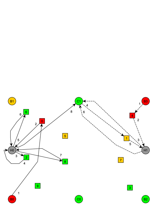
Figure 1: Allocation for ambulances of Type 1 (advanced) starting at $B0$ and $B3$.

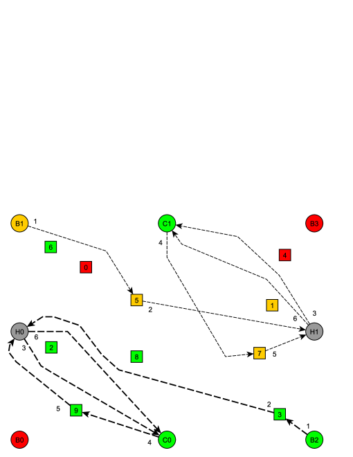
Figure 2: Allocation for ambulances of Type 2 starting at $B1$ and of Type 3 starting at $B2$.

$\Box\/$

9.2 Experiments with real data

We applied our methodology to the management of the emergency health service of Rio de Janeiro in Brazil, a large city with several millions inhabitants. The study was done in close collaboration with Rio EMS and we had access to the history of emergency calls for the period January 2016-February 2018, to the locations of the bases, to the location of the hospitals, and to the set of ambulances. The data of emergency calls can be downloaded from the webpage http://samu.vincentgyg.com/ available in menu project of home page https://www.vincentguigues.com/ mentioned in the introduction (confidential data from these calls was suppressed, so that we only report the location of the call, the time of the call, and its type).

Our implementations are available in C++17 and Matlab. The experiments were performed on a computer with AMD Ryzen 5 2600 3.4 GHz CPU, 24GB of RAM, in a Ubuntu 22.04 OS. Travel times are computed using constant speed (60 km/h) for ambulances.

We have 2 types of ambulances: ALS (Advanced Life Support) and BLS (Basic Life Support) and 4 types of calls, numbered 1, 2, 3, and 4. Any ambulance may serve any call, but every call has a priority (high or low) and may have an ambulance preference:

• type 1 call: high-priority call that should, preferably, be served by an ALS ambulance;

• type 2 call: low-priority call that should, preferably, be served by an ALS ambulance;

• type 3 call: high-priority call that any ambulance may serve;

• type 4 call: low-priority call that any ambulance may serve.

Correspondingly, to define cost allocation (2.2), we define quality of care coefficients $M_{ac}$ given in Table 2, as well as function penalization of the waiting time given by (2.1) where $\theta_{c}=4$ for calls of types 1 and 3 (high priority) and $\theta_{c}=1$ for calls of types 2 and 4 (low priority). A large (time) penalization is incurred when we send a BLS for calls that prefer an ALS and a smaller penalization is incurred when there is no ambulance preference and we send an ALS.

	1: High, ALS pref.	2: Low, ALS pref.	3: High, no pref.	4: Low, no pref.
ALS	0	0	1500	1500
BLS	6000	6000	0	0

Table 2: Quality of care coefficients $M_{ac}$. The columns correspond to the call types while the lines correspond to the ambulance types.

For the calibration of Poisson intensities for the process of emergency calls (see [22] and [23] for details of this procedure), the city was discretized into 10x10 rectangles. Using periodic probabilistic models for the process of calls with period one week and using a time discretization of the week in time windows of 30 mins, we obtain Poisson intensities (for the process of calls) $\lambda_{t,i,c}$ that are indexed by a time window $t$ of 30 mins, a rectangular subregion $i$, and a call type $c$.

We compare our 4 ambulance selection heuristics: Best Myopic (BM) from Section 4, NonMyopic (NM) from Section 5, and GHP1 and GHP2 from Section 6, with 6 heuristics from the literature: [2, 38, 45, 4, 30], as well as the Closest-Available (CA) ambulance heuristic. We use each of these heuristics H both without rolling horizon and in a rolling horizon mode, as explained in Section 3. In this latter case, heuristic H in Section 3 is one of the 10 aforementioned heuristics. For every such heuristic H used to solve the second stage problems, when an ambulance needs to be sent to a cleaning base, we choose the closest cleaning base and when an ambulance needs to be sent to a parking base, we choose the closest parking base. We generate a set of 25 scenarios of calls to compute, on these scenarios, with each policy

• the mean (Mean in the tables below), the 0.9 quantile (Q0.9 in the tables below), and the maximal (Max in the tables below) response time;

• the mean, the 0.9 quantile, and the maximal allocation cost, given by (2.2).

The 25 scenarios are generated for Friday 6pm to 8pm, where call intensities are the highest. Tables 3 and 4 respectively report the allocation costs and real response times for the 10 heuristics applied independently. Tables 5 and 6 respectively report the allocation costs and real response times for the 10 heuristics used in a rolling horizon mode, as explained in Section 3. The allocation costs and response times are reported for an EMS with 10, 12, 14, 16, 18, 20, and 30 ambulances. This allows us to see the sensitivity of the costs regarding the size of the fleet of ambulances. Such experiment can be used to calibrate an appropriate fleet size, to obtain desired allocation costs or response times. We see that our heuristics provide mean allocation costs (recall that we minimize the expected allocation cost) that are much smaller than those obtained with the 6 competing heuristics and that the rolling horizon approach described in Section 3 allows us to decrease the average allocation costs for every heuristic. Also, the allocation and response time costs tend, as expected, to decrease when the number of ambulances increase and 30 ambulances already allow us to get small response times and allocation costs for this EMS.

A	10			12			14			16
H	Mean	Q0.9	Max	Mean	Q0.9	Max	Mean	Q0.9	Max	Mean	Q0.9	Max
CA	6112	14365	38650	4467	11195	25447	3310	8145	23471	2530	6481	18506
BM	4378	11231	22660	2948	7265	14918	2177	5238	12810	1782	4319	9815
GHP1	3751	7573	17615	2729	5731	14901	2125	5026	11673	1755	4186	8567
GHP2	3580	7040	14662	2641	5590	14886	2110	4932	11673	1739	4041	7466
NM	3879	8299	18370	2789	6300	14538	2106	4995	11673	1711	4050	8304
[2]	5285	12058	39202	4018	8694	25841	3526	8144	16486	3221	7347	17548
[37]	6452	15311	36944	4721	10372	23830	4035	8709	20243	3461	7440	17548
[45]	10413	26750	52480	7825	19339	39379	6135	14684	32524	4937	11974	33201
[4]	10768	27692	49174	7959	19953	41148	5989	15345	33748	4313	10328	32458
[30]	6586	14559	37108	5133	11418	25177	4108	8830	18928	3635	8212	20228

A	18			20			30
H	Mean	Q0.9	Max	Mean	Q0.9	Max	Mean	Q0.9	Max
CA	1908	4425	19208	1505	3790	11842	844	2010	6473
BM	1518	3869	7361	1308	3583	6837	829	2010	4748
GHP1	1502	3804	8143	1296	3511	7234	829	2010	4748
GHP2	1499	3804	7181	1284	3401	7469	829	2010	4748
NM	1497	3822	6768	1292	3498	6768	829	2010	4748
[2]	2931	7065	11502	2759	6787	11502	2308	6554	9368
[37]	2960	6871	16256	2774	6823	11842	2175	6479	9137
[45]	4121	9181	26334	3094	6939	17726	2157	6352	13948
[4]	3450	8086	20922	2946	7148	20619	2070	4066	9253
[30]	3528	7896	19208	3316	7165	16256	2857	6682	13352

Table 3: Allocation costs (in seconds) for the 10 heuristics.

A	10			12			14			16
Heuristic	Mean	Q0.9	Max	Mean	Q0.9	Max	Mean	Q0.9	Max	Mean	Q0.9	Max
CA	2143	4289	8581	1482	3092	6571	1071	2203	4368	832	1805	3856
BM	1761	3369	5918	1178	2283	5080	884	1687	3202	715	1383	2866
GHP1	1861	4232	7274	1255	2770	4967	927	1777	4087	731	1410	3956
GHP2	1794	4167	8899	1220	2566	5235	932	1815	4533	751	1485	4455
NM	1824	3819	7680	1238	2513	4896	887	1707	3347	710	1398	3147
[2]	1593	3672	9426	1086	2171	6931	838	1644	5063	726	1338	3360
[37]	2157	4302	7736	1420	2965	5077	1023	2288	4205	808	1729	4198
[45]	3845	8043	12079	2734	5882	9601	2018	4365	7020	1555	3232	6800
[4]	4167	8209	13130	2915	6167	10637	2077	4440	7491	1402	3094	6615
[30]	2109	4257	7777	1438	2859	5881	1057	2246	4532	863	1742	3557

A	18			20			30
Heuristic	Mean	Q0.9	Max	Mean	Q0.9	Max	Mean	Q0.9	Max
CA	666	1264	3555	577	1107	2854	343	698	2784
BM	611	1151	2559	521	1059	2326	333	620	2154
GHP1	622	1169	3079	526	1062	3150	333	620	2154
GHP2	625	1185	3205	523	1059	3151	333	620	2154
NM	610	1144	2326	519	1059	2326	333	620	2154
[2]	628	1106	2907	584	984	2844	398	593	2183
[37]	670	1268	2929	572	1075	2857	336	626	1827
[45]	1186	2589	5083	891	2071	4142	531	1087	3112
[4]	1077	2315	4308	935	2049	3655	772	1596	3372
[30]	775	1635	3302	692	1067	3302	593	838	3191

Table 4: Response times (in seconds) for the 10 heuristics.

A	10			12			14			16
H	Mean	Q0.9	Max	Mean	Q0.9	Max	Mean	Q0.9	Max	Mean	Q0.9	Max
CA	4502	10554	27391	3398	7846	22209	2397	5697	16454	1758	4065	34341
BM	3560	8098	24118	2383	5547	16563	1849	4285	23303	1527	3561	28030
GHP1	3163	6368	29040	2252	4986	17783	1775	4071	14495	1468	3601	14772
GHP2	3610	7916	30256	2444	5115	30076	1818	3938	22447	1518	3657	18851
NM	3525	7525	23539	2447	5523	21385	1911	4257	39419	1417	3306	10359
[2]	3964	7663	19831	2779	5982	15550	2329	5578	12449	1988	4427	14022
[37]	4304	10476	21470	3317	8394	16658	2541	5923	18920	2114	4577	12449
[45]	7312	17454	36330	5650	13065	34454	4372	10056	23186	3299	7255	21602
[4]	8516	20762	64712	5777	13395	30022	4707	11219	28119	3803	8811	22523
[30]	4727	11593	23361	3534	8065	19307	2682	6601	25354	2295	5523	15659

A	18			20			30
H	Mean	Q0.9	Max	Mean	Q0.9	Max	Mean	Q0.9	Max
CA	1393	3487	12449	1179	2679	35389	627	1507	5145
BM	1261	3150	26838	1090	2573	35389	619	1452	7265
GHP1	1236	3074	23905	1066	2581	27873	620	1495	6016
GHP2	1253	3079	13212	1089	2581	32036	621	1450	6454
NM	1280	2950	26640	1143	2765	31594	616	1469	6612
[2]	1761	3973	9362	1634	3852	11020	1067	2251	6832
[37]	1725	4027	11558	1659	3790	11518	1005	2220	6375
[45]	2770	6442	17503	2229	4895	20544	1205	2608	14097
[4]	2937	6670	45173	2219	4871	18842	1433	3043	15523
[30]	1911	4315	11791	1756	3806	18902	1431	2995	10896

Table 5: Allocation costs (in seconds) for all heuristics with rolling horizon.

A	10			12			14			16
Heuristic	Mean	Q0.9	Max	Mean	Q0.9	Max	Mean	Q0.9	Max	Mean	Q0.9	Max
CA	1774	3662	8039	1327	2699	8762	877	1831	5576	662	1376	8585
BM	1577	3652	7051	998	2112	7477	770	1530	5826	624	1299	7007
GHP1	1553	3788	8198	981	2172	4984	774	1619	8202	640	1315	6535
GHP2	1729	4191	10377	1126	2550	7653	776	1556	6812	660	1327	5316
NM	1584	3672	7668	1048	2234	6945	786	1551	9855	616	1248	5556
[2]	1489	3168	8794	1078	2166	7573	814	1622	3798	704	1513	3703
[37]	1672	3437	6700	1212	2413	4808	899	1765	4531	746	1576	4174
[45]	3058	6618	11325	2318	5279	9947	1625	3464	7045	1213	2546	5846
[4]	3484	7088	14678	2302	5051	8438	1781	3805	6655	1400	2979	6350
[30]	1854	3876	9766	1364	2789	8850	922	1862	5963	782	1662	6554

A	18			20			30
Heuristic	Mean	Q0.9	Max	Mean	Q0.9	Max	Mean	Q0.9	Max
CA	533	1119	5831	474	1014	8847	282	549	5145
BM	542	1094	7489	471	951	8847	299	567	7265
GHP1	518	1076	5976	457	971	7336	305	583	6016
GHP2	536	1121	5567	468	1014	8009	310	595	6454
NM	547	1102	7326	494	963	7898	300	567	6612
[2]	612	1276	3039	573	1153	2650	424	765	2563
[37]	625	1264	3194	574	1112	2879	397	838	2449
[45]	1023	2136	4835	821	1678	3929	499	908	3524
[4]	1006	2158	10918	740	1519	3961	647	1350	5008
[30]	685	1428	3876	625	1213	4725	568	1009	5533

Table 6: Response times (in seconds) for the 10 heuristics with rolling horizon.

Finally, to try and measure the impact of the choice of the base, we compare the use of the Closest-Base Rule (CBR) for the choice of a base with the BBR rule (described in Section 8) in our heuristics BM, NM, GHP1, and GHP2. For this experiment, we take the same time window of 2 hours considered in the previous experiment and selected four zones in the west part of the city and four zones in the south part of the city (these 8 zones do not have intersection). In the first half-hour, we increased the call rates for the south zones while setting the call rates for the west zones to zero. In the last half-hour, we did the opposite, increasing call rates for the west zones and setting the call rates in the south zones to zero. In BBR, we take $\Delta$ to be 1h30.

Tables 7 and 8 report the 0.9-quantile of allocation costs, respectively without and with rolling horizon. Though for simulated data we can come up with an instance where the BBR is much better than CBR (see the next section), on this experiment based a simple modification of the real Poisson intensities, BBR and CBR provide similar performances.

	BM		GHP1		GHP2		NM
A	CBR	BBR	CBR	BBR	CBR	BBR	CBR	BBR
10	10405	10381	9527	9476	9952	9687	9300	9210
12	6096	6002	6002	6002	6002	5973	5986	5833
14	4701	4649	4725	4698	4745	4737	4654	4649
16	3875	3931	3894	3931	3931	3908	3720	3864
18	2396	2270	2466	2380	2489	2712	2342	2714
20	2288	2205	2325	2274	2297	2620	2234	2510

Table 7: 0.9-quantile (in seconds) of allocation costs for our heuristics using CBR and BBR for the choice of the base and several values for the number of ambulances.

	BM		GHP1		GHP2		NM
A	CBR	BBR	CBR	BBR	CBR	BBR	CBR	BBR
10	7855	7707	7026	6968	7533	8194	8037	8015
12	4316	4459	4654	4828	4819	5050	4597	4579
14	3576	3332	3813	3332	3332	3824	3472	3439
16	2664	2664	2735	2767	2680	2712	2664	2763
18	1956	2198	2052	1904	2051	1975	2096	2002
20	1820	1944	1831	1956	1756	1956	1719	1953

Table 8: 0.9-quantile (in seconds) of allocation costs for our heuristics using CBR and BBR for the choice of the base and a rolling horizon mode.

9.3 Experiment mixing real and simulated data

We now consider an artificial instance. In this instance, four bases and four ambulances are used, with all calls of the same priority and with every ambulance being able to serve every call. The four bases are (real) bases in the north, south, west and east regions of the city of Rio de Janeiro and the simulation begins with one ambulance at each base. We assume that the service time of each call is 45 minutes. Calls arrive in the following pattern: for the first 2 hours, say from $t=0$ to $t=2$, we have 4 calls in the South region (with time and location chosen randomly independently with uniform distribution in time and space) and no calls in the remaining 3 regions. In the next 3 hours, from $t=2$ to $t=5$, we have no calls and we repeat three times this process to obtain 4 calls in the south region for the time windows $[5,7]$ and $[10,12]$ and no calls in the time windows $[7,10]$ and $[12,15]$. We then do the same replacing the south zone with the north zone taking 4 calls in each of the three time windows $[15,17]$, $[20,22]$, and $[25,27]$ in the north zone only and no calls in time windows $[17,20]$, $[22,25]$, and $[27,30]$ in the whole city. In BBR, we take for $q(b,\Delta,\ell)$ the maximal number of calls in the corresponding time window. For this instance, if the home base rule is used, we would expect short response times for only 25% of the calls, since only the ambulances parked in the region of the call would arrive quickly. The closest base rule would perform better, since after the first set of calls, ambulances would be correctly located for the next two sets of calls, but would not be correctly relocated to the north zone when the location of calls changes to north. The Best Base Rule, on the contrary, repositions the ambulances based on an anticipation of the loads of calls and ambulance deficits in future time windows. Table 9 reports for this experiment the response times obtained for our heuristics with the home base rule and BBR for the reassignment of ambulances after service. In this example, response times are reduced by approximately 50% with BBR. It is also clear from this example, that given any positive time $\delta$, we can build a ”similar” instance, for instance with periodic calls, where the penalized response time with our heuristics and the home base rule is larger by an amount $\delta$ compared to the penalized response time with these heuristics combined with BBR for ambulance reassignment.

	HBR	BBR
CA	1505	734
BM	1468	734
GHP1	1468	734
GHP2	1468	734
NM	1468	709

Table 9: Response times obtained with our ambulance selection heuristics combined with either the Home Base Rule (HBR) or the Best Base Rule (BBR) for ambulance reassignment for 4 ambulances.

References

- [1] R. Alanis, A. Ingolfsson, and B. Kolfal. A Markov chain model for an EMS system with repositioning. Production and Operations Management, 22(1):216–231, 2013.
- [2] T. Andersson and P. Värbrand. Decision support tools for ambulance dispatch and relocation. Journal of the Operational Research Society, 58(2):195–201, 2007.
- [3] D. Bandara, M. E. Mayorga, and L. A. McLay. Optimal dispatching strategies for emergency vehicles to increase patient survivability. International Journal of Operational Research, 15(2):195–214, 2012.
- [4] D. Bandara, M. E. Mayorga, and L. A. McLay. Priority dispatching strategies for EMS systems. Journal of the Operational Research Society, 65:572–587, 2014.
- [5] V. Bélanger, Y. Kergosien, A. Ruiz, and P. Soriano. An empirical comparison of relocation strategies in real-time ambulance fleet management. Computers and Industrial Engineering, 94:216–229, 2016.
- [6] G. N. Berlin and J. C. Liebman. Mathematical analysis of emergency ambulance location. Socio-Economic Planning Sciences, 8(6):323–328, 1974.
- [7] L. Brotcorne, G. Laporte, and F. Semet. Ambulance location and relocation models. European Journal of Operational Research, 147(3):451–463, 2003.
- [8] T. H. Burwell, J. P. Jarvis, and M. A. McKnew. Modeling co-located servers and dispatch ties in the hypercube model. Computers and Operations Research, 20(2):113–119, 1993.
- [9] R. L. Church and C. S. ReVelle. The maximal covering location problem. Papers of the Regional Science Association, 32:101–118, 1974.
- [10] M. S. Daskin. A maximum expected covering location model: Formulation, properties and heuristic solution. Transportation Science, 7(1):48–70, 1983.
- [11] M. S. Daskin and E. H. Stern. A hierarchical objective set covering model for Emergency Medical Service vehicle deployment. Transportation Science, 15(2):137–152, 1981.
- [12] D. Degel, L. Wiesche, S. Rachuba, and B. Werners. Time-dependent ambulance allocation considering data-driven empirically required coverage. Health Care Management Science, 18:444–458, 2015.
- [13] E. Erkut, A. Ingolfsson, T. Sim, and G. Erdoğan. Computational comparison of five maximal covering models for locating ambulances. Geographical Analysis, 41:43–65, 2009.
- [14] J. A. Fitzsimmons. A methodology for emergency ambulance deployment. Management Science, 19(6):627–636, 1973.
- [15] M. Gendreau, G. Laporte, and F. Semet. Solving an ambulance location model by Tabu Search. Location Science, 5(2):75–58, 1997.
- [16] M. Gendreau, G. Laporte, and F. Semet. A dynamic model and parallel tabu search heuristic for real-time ambulance relocation. Parallel Computing, 27(12):1641–1653, 2001.
- [17] M. Gendreau, G. Laporte, and F. Semet. The maximal expected coverage relocation problem for emergency vehicles. Journal of the Operational Research Society, 57(1):22–28, 2006.
- [18] J. Goldberg, R. Dietrich, J. M. Chen, M. G. Mitwasi, T. Valenzuela, and E. Criss. Validating and applying a model for locating emergency medical vehicles in Tucson, AZ. European Journal of Operational Research, 49(3):308–324, 1990.
- [19] J. Goldberg and L. Paz. Locating emergency vehicle bases when service time depends on call location. Transportation Science, 25(4):264–280, 1991.
- [20] J. Goldberg and F. Szidarovszky. Methods for solving nonlinear equations used in evaluating emergency vehicle busy probabilities. Operations Research, 39(6):903–916, 1991.
- [21] V. Guigues, A. Kleywegt, V. H. Nascimento, Victor Salles, and Thais Viana. Management and visualization tools for emergency medical services. arXiv, 2024.
- [22] V. Guigues, A. J. Kleywegt, G. Amorim, A. M. Krauss, and V. H. Nascimento. LASPATED: A Library for the Analysis of SPAtio-TEmporal Discrete Data. arXiv:2401.04156v2 [stat.ME], 2023.
- [23] V. Guigues, A. J. Kleywegt, G. Amorim, A. M. Krauss, and V. H. Nascimento. LASPATED: A Library for the Analysis of SPAtio-TEmporal Discrete Data (User Manual). arXiv:2407.13889 [stat.CO], 2023.
- [24] V. Guigues, A. J. Kleywegt, and V. H. Nascimento. Operation of an ambulance fleet under uncertainty. arXiv:2203.16371v2 [math.OC], 2022.
- [25] S. G. Henderson and A. J. Mason. Estimating ambulance requirements in Auckland, New Zealand. In Proceedings of the 1999 Winter Simulation Conference, volume 2, pages 1670–1674, 1999.
- [26] S. G. Henderson and A. J. Mason. Ambulance service planning: Simulation and data visualisation. In M. Brandeau, F. Sainfort, and W. Pierskalla, editors, Operations Research and Health Care: A Handbook of Methods and Applications, International Series in Operations Research and Management Science 70, chapter 4, pages 77–102. Kluwer, Dordecht, 2004.
- [27] E. D. Hill, J. L. Hill, and L. M. Jacobs. Planning for emergency ambulance service systems. The Journal of Emergency Medicine, 1:331–338, 1984.
- [28] K. Hogan and C. S. Revelle. Concepts and applications of backup coverage. Management Science, 32(11):1434–1444, 1986.
- [29] A. Ingolfsson, S. Budge, and E. Erkut. Optimal ambulance location with random delays and travel times. Health Care Management Science, 11:262–274, 2008.
- [30] C. J. Jagtenberg, S. Bhulai, and R. D. Van der Mei. An efficient heuristic for real-time ambulance redeployment. Operations Research for Health Care, 12(4):27–35, 2015.
- [31] C. J. Jagtenberg, S. Bhulai, and R. D. Van der Mei. Dynamic ambulance dispatching: Is the closest-idle policy always optimal? Operations Research for Health Care, 20(4):517–531, 2017.
- [32] C. J. Jagtenberg, P. L. Van den Berg, and R. D. Van der Mei. Benchmarking online dispatch algorithms for Emergency Medical Services. European Journal of Operational Research, 258(2):715–725, 2017.
- [33] J. P. Jarvis. Approximating the equilibrium behavior of multi-server loss systems. Management Science, 31(2):235–239, 1985.
- [34] V. A. Knight, P. R. Harper, and L. Smith. Ambulance allocation for maximal survival with heterogeneous outcome measures. Omega, 40:918–926, 2012.
- [35] R. C. Larson. A hypercube queuing model for facility location and redistricting in urban emergency services. Computers and Operations Research, 1:67–95, 1974.
- [36] R. C. Larson. Approximating the performance of urban emergency service systems. Operations Research, 23(5):845–868, 1975.
- [37] S. Lee. The role of preparedness in ambulance dispatching. Journal of the Operational Research Society, 62(10):1888–1897, 2011.
- [38] S. Lee. The role of centrality in ambulance dispatching. Decision Support Systems, 54(1):282–291, 2012.
- [39] X. Li and C. Saydam. Balancing ambulance crew workloads via a tiered dispatch policy. Pesquisa Operacional, 36(3):399–419, 2016.
- [40] A. J. Mason. Simulation and real-time optimised relocation for improving ambulance operations. In B. T. Denton, editor, Handbook of Healthcare Operations Management: Methods and Applications, International Series in Operations Research and Management Science 184, chapter 11, pages 289–317. Springer, New York, 2013.
- [41] M. S. Maxwell, S. G. Henderson, and H. Topaloglu. Ambulance redeployment: An approximate dynamic programming approach. In M. D. Rossetti, R. R. Hill, B. Johansson, A. Dunkin, and R. G. Ingalls, editors, Proceedings of the 2009 Winter Simulation Conference, pages 1850–1860, 2009.
- [42] M. S. Maxwell, S. G. Henderson, and H. Topaloglu. Tuning approximate dynamic programming policies for ambulance redeployment via direct search. Stochastic Systems, 3(2):322–361, 2013.
- [43] M. S. Maxwell, E. C. Ni, C. Tong, S. G. Henderson, H. Topaloglu, and S. R. Hunter. A bound on the performance of an optimal ambulance redeployment policy. Operations Research, 62(5):1014–1027, 2014.
- [44] M. S. Maxwell, M. Restrepo, S. G. Henderson, and H. Topaloglu. Approximate dynamic programming for ambulance redeployment. INFORMS Journal on Computing, 22(2):266–281, 2010.
- [45] M. E. Mayorga, D. Bandara, and L. A. McLay. Districting and dispatching policies for emergency medical service systems to improve patient survival. IIE Transactions on Healthcare Systems Engineering, 3(1):39–56, 2013.
- [46] R. Nair and E. Miller-Hooks. Evaluation of relocation strategies for emergency medical service vehicles. Transportation Research Record, 2137:63–73, 2009.
- [47] J. F. Repede and J. J. Bernardo. Developing and validating a decision support system for locating emergency medical vehicles in Louisville, Kentucky. European Journal of Operational Research, 75:567–581, 1994.
- [48] M. Restrepo, S. G. Henderson, and H. Topaloglu. Erlang loss models for the static deployment of ambulances. Health Care Management Science, 12(67):67–79, 2009.
- [49] C. ReVelle and K. Hogan. The maximum availability location problem. Transportation Science, 23(3):192–200, 1989.
- [50] D. A. Schilling, D. J. Elzinga, J. Cohon, R. L. Church, and C. S. ReVelle. The TEAM/FLEET models for simultaneous facility and equipment siting. Transportation Science, 13(2):163–175, 1979.
- [51] V. Schmid. Solving the dynamic ambulance relocation and dispatching problem using approximate dynamic programming. European Journal of Operational Research, 219:611–621, 2012.
- [52] V. Schmid and K. F. Doerner. Ambulance location and relocation problems with time-dependent travel times. European Journal of Operational Research, 207:1293–1303, 2010.
- [53] P. Sorensen and R. Church. Integrating expected coverage and local reliability for emergency medical services location problems. Socio-Economic Planning Sciences, 44(1):8–18, 2010.
- [54] C. Swoveland, D. Uyeno, I. Vertinsky, and R. Vickson. Ambulance location: A probabilistic enumeration approach. Management Science, 20(4):686–698, 1973.
- [55] C. Swoveland, D. Uyeno, I. Vertinsky, and R. Vickson. A simulation-based methodology for optimization of ambulance service policies. Socio-Economic Planning Sciences, 7(6):697–703, 1973.
- [56] Luca Talarico, Frank Meisel, and Kenneth Sörensen. Ambulance routing for disaster response with patient groups. Computers and Operations Research, 56:120–133, 2015.
- [57] C. Toregas, R. Swain, C. ReVelle, and L. Bergman. The location of emergency service facilities. Operations Research, 19(6):1363–1373, 1971.
- [58] T. C. Van Barneveld, S. Bhulai, and R. D. Van der Mei. The effect of ambulance relocations on the performance of ambulance service providers. European Journal of Operational Research, 252:257–269, 2016.
- [59] T. C. Van Barneveld, S. Bhulai, and R. D. Van der Mei. A dynamic ambulance management model for rural areas: Computing redeployment actions for relevant performance measures. Health Care Management Science, 20:165–186, 2017.
- [60] R. A. Volz. Optimum ambulance location in semi-rural areas. Transportation Science, 5(2):193–203, 1971.