Distributed Binary Optimization with In-Memory Computing:
An Application for the SAT Problem

Abstract

In-memory computing (IMC) has been shown to be a promising approach for solving binary optimization problems while significantly reducing energy and latency. Building on the advantages of parallel computation, we propose an IMC-compatible parallelism framework inspired by parallel tempering (PT), enabling cross-replica communication to improve the performance of IMC solvers. This framework enables an IMC solver not only to improve performance beyond what can be achieved through parallelization, but also affords greater flexibility for the search process with low hardware overhead. We justify that the framework can be applied to almost any IMC solver. We demonstrate the effectiveness of the framework for the Boolean satisfiability (SAT) problem, using the WalkSAT heuristic as a proxy for existing IMC solvers. The resulting PT-inspired cooperative WalkSAT (PTIC-WalkSAT) algorithm outperforms the traditional WalkSAT heuristic in terms of the iterations-to-solution in 76.3% of the tested problem instances and its naïve parallel variant (PA-WalkSAT) does so in 68.4% of the instances. An estimate of the energy overhead of the PTIC framework for two hardware accelerator architectures indicates that in both cases the overhead of running the PTIC framework would be less than 1% of the total energy required to run each accelerator.

I Introduction

In recent years, in-memory computing (IMC) has demonstrated promising results in solving binary optimization problems [1, 2, 3, 4, 5], showing significant improvements in terms of reduced energy consumption, chip area, and time-to-solution. The small design and low-energy consumption of IMC hardware makes it a natural candidate for using multiple IMC cores to build highly parallelized optimization solvers. Parallelism is a well-established strategy for improving the performance of optimization solvers, from employing the naïve strategy of running parallel independent solver replicas with different initial solutions or random seeds to using more-advanced parallel heuristics [6, 7, 8].

Earlier work [6, 9, 10, 11, 12] on cooperative parallelism heuristics, where multiple replicas of solvers can communicate with each other, has shown that these heuristics can significantly outperform naïve parallelism strategies, at the cost of increased complexity and potentially higher energy consumption overhead. In this paper, we propose a simple algorithmic framework that leverages inter-replica communication across IMC solvers with a minimal increase in energy overhead. Our proposed method is inspired by the parallel tempering (PT) algorithm, a technique used extensively in statistical physics and computational optimization [13, 14, 15, 16]. The PT algorithm runs multiple parallel replicas at different temperatures, periodically exchanging solutions between pairs of replicas at adjacent temperatures. The temperature parameter modulates each replica’s exploration versus exploitation strategy. Higher-temperature replicas are better at exploring the solution space and can easily overcome local optima, whereas lower-temperature replicas are greedier and converge more quickly by closely following energy gradients [17]. The replica-exchange mechanism enables the transfer of information along the chain of replicas, combining the strengths of both approaches. The PT algorithm has been successfully applied to various optimization problems [16, 18, 19, 20, 21]; for example, relevant to this work, a CPU-based Boolean satisfiability (SAT) problem [22] solver using PT as its algorithmic engine was used by the team who won the 2016 MAXSAT competition [16].

Our proposed framework is designed to run multiple IMC solvers in parallel, each representing a single replica in the PT algorithm framework. In-memory computing solvers must have a configurable parameter that represents the replica’s temperature, and be able to communicate with the other solvers to perform replica exchanges. In this context, the temperature refers to any parameter that has an effect on the balance between exploration and exploitation. Some examples of parameters that could be used as replica temperature analogues are the noise threshold in WalkSAT heuristics, the size of the tabu tenure in tabu heuristics, and the solution restart frequency. Almost every stochastic local search (SLS) algorithm for binary optimization problems has similar tunable parameters, regardless of the hardware architecture, which highlights the framework’s broad applicability.

The framework is natively parallel, and generalizes concepts underlying the PT algorithm and other cooperative search algorithms; we thus refer to it as “PT-inspired cooperative search” or the “PTIC framework” for short. The PTIC framework can support a wide range of hardware accelerators and has a very low energy overhead, which is discussed in detail in Sec. III.3.

To demonstrate the effectiveness of the PTIC framework, we apply it to the SAT problem. The SAT problem was the first identified NP-complete problem [22, 23]. It is a problem of significant practical importance with many industrial applications, for example, in cryptography [24], large-circuit verification [25], and AI planning [26]. Due to the ubiquity of SAT applications [27], several IMC SAT solvers have recently been proposed [3, 4, 5, 28, 29], the majority of them based on the WalkSAT heuristic [30].

In this work, we use the PTIC framework to build a SAT solver where the replicas implement the WalkSAT heuristic [30], as the WalkSAT heuristic is a performant heuristic that maps well to IMC hardware [29]. Additionally, the WalkSAT heuristic is one of the most well-known and studied SAT-solving heuristics, with fast, open source CPU versions freely available [31]. By integrating the PTIC framework with the WalkSAT heuristic, we develop a distributed algorithm we call the “PTIC-WalkSAT” algorithm.

To summarize, the study makes the following contributions.

1. A parallelization framework, the PTIC framework, is proposed to improve the performance of IMC solvers for binary optimization with minimal energy consumption overhead.

2. We apply the PTIC framework to build a SAT solver using the WalkSAT heuristic. The PTIC-WalkSAT algorithm is benchmarked to empirically prove its effectiveness with extensive computational experiments.

3. A hardware energy model is proposed to evaluate the energy consumption overhead of implementing the PTIC framework on two different IMC hardware architectures.

This paper is organized as follows. Section II introduces the SAT problem, the WalkSAT heuristic, and PT. In Sec. III, we describe the SAT problem instances used for benchmarking and the PTIC-WalkSAT algorithm, as well as two benchmarking-related techniques: the evaluation metrics and the simulation environment. Section IV presents the full computational results. In Sec. V, further analysis and discussion are provided. Section VI gives a brief summary of our work, concluding the article. An appendix provides additional information on the PTIC-WalkSAT algorithm and our full benchmarking results.

II Background and Preliminaries

Parallel tempering is a Markov chain Monte Carlo (MCMC) method [13, 14] for obtaining the system configuration that has the lowest energy. In highly complex physical systems such as spin glasses, it is crucial to investigate the distribution of configurations at thermal equilibrium. This requires sampling from the system configurations associated with the lowest energy from the Boltzmann distribution. However, directly deriving samples from this distribution is a nontrivial task, which led to the development of MCMC methods. The core principle of MCMC methods is that, by properly engineering the Markov chain, it will converge to the stationary probability distribution, which is the target distribution, regardless of the initial configuration. The step of obtaining a sample from the Markov chain based on the current state is referred to as performing an “MC update”. Using the Metropolis–Hastings (MH) algorithm [32, 33] to perform the MC update results in an MCMC method that serves this purpose. Theoretically, if the MH algorithm runs infinitely long, it can reach all the configurations including the global minimum energy configuration, which is the most stable state of the system. Unfortunately, in practice, the algorithm could become trapped among local minima for two reasons: the algorithm cannot execute indefinitely in practice and the energy landscape of a system could be very rough at a low system temperature. A “rough” energy landscape is one where many local minima are separated by high energy barriers, making it very hard for the MH algorithm to reach the global minimum [13].

To overcome energy barriers, PT runs the MH algorithm on replicas of the system, denoted by the list $\mathcal{R}=\{r_{1},r_{2},...,r_{\kappa}\}$, each of which is permanently associated with a specific index $i$ and is characterized by a unique temperature from the list $\mathcal{T}=\{T_{1},T_{2},...,T_{\kappa}\}$, with $T_{1}<T_{2},\ldots,<T_{\kappa}$, where $\kappa$ is the total number of replicas and temperatures, respectively. Let $x_{i}\in\{0,1\}^{n}$ denote the incumbent system configuration associated with replica $r_{i}$, where $n$ is the number of system variables. Even if replica exchanges are performed during the PT process, $r_{i}$ always refers to the $i$-th replica, maintaining its identity throughout the simulation. Similarly, $E_{i}$ refers to the energy of the incumbent configuration $x_{i}$. Mapping $\mathcal{E}$: $\{0,1\}^{n}\to\mathbb{R}$ returns the energy value given a system configuration. In other words, we have $E_{i}=\mathcal{E}(x_{i})$. After a predetermined number of MC updates at each temperature, configurations of the neighbouring replicas $r_{i-1}$ and $r_{i}$ are exchanged with the probability

$$P(E_{i-1},T_{i-1}\leftrightarrow{E_{i},T_{i}})=\mathrm{min}(1,e^{\Delta\beta\Delta E}),$$ (1)

where $\Delta\beta=1/T_{i}-1/T_{i-1}$ and $\Delta E=E_{i}-E_{i-1}$, with $\Delta E$ representing the energy difference between the incumbent configurations in the replicas $r_{i-1}$ and $r_{i}$. The replica-exchange mechanism allows a lower-energy configuration in a higher-temperature replica to be transferred to a lower-temperature replica for intensification. Conversely, it enables a higher-energy configuration in a lower-temperature replica to be moved to a higher temperature for diversification. A “sweep” is defined as the period during which each replica independently updates all degrees (i.e., variables) of the system once. After completing one or a chosen number of sweeps, a tentative replica exchange is performed. One run of PT could conduct many sweeps before convergence. In practice, a limit $S$ is put on the number of sweeps to prevent infinite loops from occurring. Other notation not defined elsewhere for PT is as follows:

• Rand(): a function used to generate a value in the interval $[0,1]$ following some probability distribution (e.g., uniform);

• $Q$: the maximum number of steps (i.e., updates) performed within one sweep;

• $B$: the global variable used to track the best configuration, initialized with a starting random configuration;

• $E$: the energy value associated with the best configuration.

Algorithm 1 gives the pseudocode for the standard PT procedure.

Algorithm 1  The Standard Framework of Parallel Tempering

1:Initialize global variables $\mathcal{R}$, $\mathcal{T}$, $B$, $E$;

2:for each replica $r_{i}$ do

3:     Initialize the configuration $x_{i}$;

4:end for

5:for sweep $s=1,\ldots,S$ do

6:     for each replica $r_{i}$ do

7:         Perform a sweep to update the configuration $x_{i}$;

8:         if $E_{i}==0$ then

9:              return the configuration $x_{i}$;

10:         else if $E_{i}<E$ then

11:              $B=x_{i}$, $E=E_{i}$;

12:         end if

13:     end for

14:     for each pair of neighbouring replicas $(i,j=i+1)$ do

15:         Compute the acceptance probability $P(E_{i},T_{i}\leftrightarrow{E_{j},T_{j}})$ as per Eq. (1);

16:         if Rand() $<P$ then

17:              Swap the replicas $r_{i}$ and $r_{j}$;

18:         end if

19:     end for

20:end for

21:return $B,E$

III Methods

III.1 The PTIC Framework

The PTIC framework uses an IMC binary optimization solver to perform local updates to the configurations of the replicas. The “local update” can be seen as a step used to find a new configuration given the incumbent one. For binary optimization problems, any mapping $\{0,1\}^{n}\to\{0,1\}^{n}$ can serve as the local update, where $n$ is the number of binary variables. However, there is an additional requirement for a mapping to be a valid local update: the mapping must be probabilistic, with the extent of this probabilistic behaviour governed by a noise parameter $\eta$. The parameter $\eta$ plays a crucial role in most heuristic solvers, as it helps them escape local minima. Consequently, this parameter is commonly found in many IMC solvers [2, 3, 4], which reflects the generality of satisfying the requirements of the local update. We use $\mathcal{L}_{\eta}$ to represent that the local update employs $\eta$, whereas $\mathcal{L}$ refers to the general case that does not specify the amount of noise.

The default PT implementation uses the temperature of each replica to calculate the MH parameter used to accept or reject local updates: high-temperature replicas typically accept most configuration proposals whereas low-temperature replicas tend to accept better proposals. In the PTIC framework, the temperature of each replica is reframed as the noise parameter $\eta$. With high values of $\eta$, the local update typically makes a random move, and with low values of $\eta$, it tends to move to a better configuration. The notion of a sweep in the PTIC framework is different from that of standard PT, as within a sweep of the PTIC framework, not every variable needs to be updated. Instead, we perform only a fixed number of local updates, which could leave some of the variables unchanged. To distinguish a sweep of the framework from a standard sweep, we call it an “episode”. At the end of each episode, tentative replica exchanges are performed. As illustrated in Fig. 1, at the end of every episode, each pair of adjacent replicas can exchange their configurations with a probability defined in Eq. (1), where the energy $E_{i}$ refers to the number of violated clauses associated with the last configuration found by the replica $r_{i}$ before the episode ends.

Figure 1: Replica exchange visualization

A formal description of the PTIC framework is presented as Algorithm 2. We use $\mathcal{P}$ to denote the binary optimization problem to be solved.

Algorithm 2  The PTIC Framework

1:Function PTIC($\mathcal{P},\mathcal{L}$):

2:Initialize $\mathcal{R}$, $\mathcal{T}$, $B$, $E$;

3:Initialize a counter $s=0$;

4:while $E>0$ and $s<S$ do

5:     for $i=1,2,\ldots,\kappa$ do

6:         $x_{i},E_{i}=\text{Episode}(x_{i},Q,\mathcal{L}_{T_{i}})$;

7:         if $E_{i}==0$ then

8:              Return $x_{i}$;

9:         else if $E_{i}<E$ then

10:              $B=x_{i}$, $E=E_{i}$;

11:         end if

12:     end for

13:     for $i=1,2,\ldots,\kappa-1$ do

14:         Compute the acceptance probability $P(E_{i},T_{i}\leftrightarrow{E_{i+1},T_{i+1}})$ as per Eq. (1);

15:         if Rand() $<P$ then

16:              Swap the replicas $r_{i}$ and $r_{j}$;

17:         end if

18:     end for

19:     $s\leftarrow s+1$;

20:end while

21:return $B,E$

III.2 Applying the PTIC Framework to the SAT Problem

III.2.1 The Boolean Satisfiability Problem

The SAT problem can be formally described as follows. Given a propositional formula $\mathcal{F}$, expressed in the conjunctive normal form, or “CNF”, formulation defined by a set of variables $\mathcal{V}$ and a set of clauses $\mathcal{C}$, solving the SAT problem amounts to finding an assignment to the variables that renders all the clauses true. The following equation is an example of a SAT problem that is composed of four variables and four clauses.

$$\mathcal{F}(x_{1},x_{2},x_{3},x_{4})=(x_{1}\lor\neg x_{2}\lor x_{4})\land(x_{2}\lor\neg x_{3})\land(x_{3}\lor x_{4})\land(\neg x_{1}\lor\neg x_{3})$$ (2)

In general, an assignment to the SAT problem is a set of binary values that specifies whether a variable should have a value of 1 or 0. In our example, $x_{1},x_{2},x_{3},x_{4}=0,0,0,0$ is an assignment to $\mathcal{F}(x_{1},x_{2},x_{3},x_{4})$ such that it makes true three out of four clauses. An assignment that makes all the clauses true is considered a solution to the problem, for example, $x_{1},x_{2},x_{3},x_{4}=0,1,0,1$ is a solution to the problem represented by the formula $\mathcal{F}$.

III.2.2 The WalkSAT Heuristic

The seminal paper by Selman, Kautz, Cohen, et al. [30] introduces WalkSAT heuristics, which generally begin with an initial configuration updated by flipping one variable at each iteration of a loop. One of the critical steps of WalkSAT heuristics is to decide which variable to flip, which depends on a scoring function. With different scoring functions, different versions of WalkSAT heuristics can be derived. In particular, in our study, we use the break value to score a candidate variable as the default version implemented in the codebase [31] uses the break value. The term “break value” refers to the number of newly violated clauses with respect to a variable, that is, the number of clauses that are satisfied in the current solution, but will become violated upon flipping the variable. If not otherwise specified, “WalkSAT heuristic” refers to the version that uses the break value throughout the rest of the paper. Aside from the scoring function, the walk probability is a simple yet critical setting [30] because it prevents the heuristic from always performing a greedy move with respect to the break value, which could easily cause the heuristic to become trapped in local optima. The pseudocode of the heuristic is presented in Algorithm 3.

Algorithm 3  The WalkSAT Heuristic

1:Function WalkSAT($\mathcal{C},x,Q,\eta$):

2:Initialize $q=0$;

3:while any violated clause with respect to $x$ and $q<Q$ do

4:     Randomly choose a violated clause;

5:     Initialize $l^{\prime}$ to $0$ and $z^{\prime}$ to a large number;

6:     for $l$ in the literals of the chosen clause do

7:         Compute the break value for $l$, denoted as $z(l)$;

8:         if $z^{\prime}>z(l)$ then

9:              $z^{\prime}=z(l)$, $l^{\prime}=l$;

10:         end if

11:     end for

12:     if Rand() $<\eta$ then

13:         Randomly choose a variable from the clause to flip;

14:     else

15:         Choose the variable $\mathrm{abs}(l^{\prime})$ to flip;

16:     end if

17:     Update $x$ to align with the flipped variable;

18:     $q\leftarrow q+1$;

19:end while

III.2.3 The PTIC-WalkSAT Algorithm

In order to embed the WalkSAT heuristic into the PTIC framework, the local update $\mathcal{L}$ that captures its main features must be identified. Since the key component of the WalkSAT heuristic is to decide the variable to flip and perform the flip at each iteration, we can define $\mathcal{L}_{\eta}$ as one iteration of the WalkSAT heuristic with the walk probability $\eta$. The local update is equivalent to executing lines 4 through 17 of Algorithm 3. The local update can also be referred to as a“step” or “iteration” in the context of the PTIC-WalkSAT algorithm. The local update is valid as it satisfies the two conditions defined in Sec. III.1: flipping a variable is a mapping $\{0,1\}^{n}\to\{0,1\}^{n}$, and the walk probability provides randomness to the mapping. As for the notion of temperature, we reframe the walk probability as the temperature, because the walk probability manages the degree of greediness in performing the local update. In other words, in the context of the PTIC-WalkSAT algorithm, temperature and walk probability can be considered equivalent. Temperatures are bound between $0.0<T_{1},T_{2},\dots,T_{\kappa}\leq 1.0$ because $\eta$ is a probability.

III.3 Hardware Implementation for the PTIC Framework

The generic nature of the PTIC framework makes it suitable for implementation on a variety of hardware accelerator platforms. In what follows, we wish to sketch possible implementations and consider the overhead of the PTIC framework for two example in-memory accelerators that can be used to solve SAT problems. Both accelerators utilize memristor crossbar arrays to perform massively parallel computation of gradients. The first accelerator, depicted in Fig. 2(a), implements a gradient-decent optimization of polynomial unconstrained binary optimization (PUBO) problems [34]. Boolean satisfiability problems can generally be expressed as PUBO problems by translating their clauses into the generic polynomial cost function $E=\sum_{ij}A_{ij}x_{i}x_{j}+\sum_{kmn}B_{kmn}x_{k}x_{m}x_{n}+\ldots$. Here, $x_{i}=\{0,1\}$ are the Boolean variables and $A_{ij}$, $B_{kmn},\ldots$ are the linear coefficients for polynomials of a given order. The memristor crossbar is employed for calculating gradients of the PUBO cost function, which is used to decide whether a specific variable needs to be flipped to minimize the number of unsatisfied clauses. To escape local minima, an analog noise signal is added to the gradients. In the accelerator, this is achieved using an array of digital-to-analog-converters (DAC), which is driven by a pseudo-random number generator (labelled “PRNG” in Fig. 2). The magnitude of the generated analog noise signal is adjustable through a voltage signal provided by an additional DAC. Based on these noisy gradients, the register entries storing the Boolean variables are then flipped. For small-scale problems, such PUBO accelerators have shown to be able to solve SAT problems while consuming only a few milliwatts of electrical power [34]. These accelerators can be adapted to the PTIC framework, where each replica is implemented as a new, separate PUBO accelerator. In this case, the temperature of each replica is given by the strength of the injected noise signal. To support the PTIC framework, a PUBO accelerator must be extended so as to calculate the overall cost for each replica. In addition, a central processing element is required that enables the replica-exchange process by comparing each pair of temperature-adjacent replicas.

To evaluate the PUBO cost function, determining the overall cost for each replica is needed in order to calculate the acceptance probability in Eq. (1) during each replica exchange. In principle, the cost function can be evaluated inside the crossbar array at the expense of having a larger crossbar. As shown in Fig. 2(a), an additional crossbar column is used to sum the cost terms. Additional crossbar rows are also needed to calculate the cost of the individual clauses. Under the worst-case assumptions (i.e., when none of the cost terms are identical to the gradients of other clauses), twice the number of crossbar rows would be required. The output signal of this additional crossbar column is then sampled by an analog-to-digital converter (ADC) with a resolution of $\log_{2}(number\,of\,clauses)$. The PUBO cost for each replica is evaluated in the central processing element that calculates the acceptance probability, performs the replica exchange, and updates the temperature for each replica. The temperature signal is then provided to the control DAC to adjust the magnitude of the analog noise signal within the replicas.

As the second example in-memory accelerator architecture, we consider a content addressable memory (CAM) based SAT solver (CAMSAT), depicted in Fig. 2(b). The CAMSAT accelerator implements a WalkSAT-like heuristic using crossbar arrays [3]. This architecture consists of two crossbar arrays, where the first is used to evaluate violations of the SAT clauses. The output of the crossbar arrays uses a binary signal to indicate whether the clauses mapped to the respective row of the array are violated by the current variable configuration. This signal is passed to the second crossbar array, which is the transpose of the first array. The output of this second crossbar array indicates how many clauses become satisfied when flipping each of the variables (the “make value”) during one iteration. A winner-takes-all (labelled “WTA” Fig. 2(b)) circuit then selects the variable with the highest make value and flips its value. As with the PUBO architecture, an analog noise signal is added to aid the solver in escaping local minima. Adapting this architecture to the PTIC framework requires the calculation of the cost function, which is given by the number of violated clauses. This can be achieved within the second crossbar array using an additional row that sums the input values. The output of this row is then digitized with an ADC with a $\log_{2}(number\,of\,clauses)$-bit resolution. As in the case of the PUBO accelerators, the replica temperature is given by the magnitude of the injected noise signal. The central processing unit used to perform the replica exchange is identical to that of the discussed PUBO architecture.

Figure 2: Exemplary hardware architectures for realizing the PTIC framework within (a) a PUBO and (b) a CAMSAT hardware accelerator for solving SAT problems. Peripherals added to support the PTIC framework are highlighted in yellow.

To estimate the potential overhead of adapting these accelerator architectures to the PTIC framework, we compare the energy consumption of an individual accelerator system with that of the additional peripheral components discussed. For the PUBO accelerator, we estimate that the overhead from the PUBO cost calculation would double the energy consumption of the crossbar array $E_{\text{xbar}}$ each time a replica exchange is performed, where the Boltzmann factors in Eq. (1) are evaluated. In addition, the ADC consumes $E_{\text{ADC}}$ at each evaluation. Of note, the cost calculation is required only during replica exchanges, such that the section of the crossbar array dedicated to the cost evaluation and the ADC are activated only every $Q$ iterations. The average energy overhead from the cost evaluation per solver iteration is thus $(E_{\text{xbar}}+E_{\text{ADC}})/Q$. In what follows, the subscripts “stat” and “dyn” represent the static and dynamic energy, respectively, where static energy is consumed continuously, while dynamic energy is consumed only during a specific operation. The central processing unit can be realized using vector processing units (VPU) that are similarly employed in electronic AI accelerators and digital signal processors. Such VPUs can perform parallel linear and nonlinear operations. The energy consumption of VPUs is estimated to be $E_{\text{VPU,stat}}+E_{\text{VPU,dyn}}/Q$ per iteration. As an example, we estimate the total PTIC framework’s energy overhead for the PUBO architecture presented in [34], designed to solve 20-variable 3SAT problems. In the referenced PUBO architecture, the total energy used is $1.3$ pJ/iteration. For the crossbar array, ADC, and VPU, we estimate energy consumption per iteration based on values obtained from the literature for the same technology node to be $E_{\text{ADC, dyn}}=1.5$ pJ [35], $E_{\text{VPU,dyn}}=2.2$ pJ, $E_{\text{VPU,stat}}=0.25$ pJ [36], and $E_{\text{xbar}}=0.35$ pJ. Assuming that replica exchanges occur every $Q=1000$ iterations, the PTIC framework’s energy overhead constitutes $0.0086$ pJ/iteration, equivalent to $0.65$% of the total energy consumption.

For the CAMSAT accelerator, the energy overhead can be estimated in a similar fashion. We assume that the overhead from the cost function evaluation is similar to the energy consumption of a single row in the second crossbar array. In contrast to cost function evaluations using the PUBO accelerator, each row is driven by the same input signals as the gradient calculation, such that we cannot assume it to be turned off outside of replica exchanges. The overhead of the other peripheral components is identical to that of the PUBO accelerator, but must be adjusted for the longer iteration time of the CAMSAT accelerator. As an example, as we did in the case of the PUBO architecture, we estimate the energy overhead for a CAMSAT solver for 20-variable 3SAT problems, where the average energy is approximately $2.6$ pJ/iteration. For the crossbar arrays’ energy, we estimate $E_{\text{xbar}}=0.02$ pJ/iteration. Assuming that the replica exchange occurs every $Q=1000$ iterations, the PTIC framework’s energy overhead constitutes $0.01965$ pJ/iteration, which is equivalent to $0.76$% of the total energy consumption.

III.4 Benchmarking Methodology

III.4.1 The Problem Instances

The problem instances used in our benchmarking experiments were chosen to be hard for WalkSAT algorithms. There are four groups of instances. Group-1 was generated from well-known semi-prime factoring problems [37]. The number of variables in the instances ranges from 82 to 100 variables, and the number of clauses ranges from 1177 to 2642. Group-2 comprises statistically hard random 4SAT problems, each of which has a quietly planted solution [38]. Each of the instances has 1000 clauses and 100 variables. To have statistically hard instances, the problems were generated at the computational phase transition threshold [39]. A similar approach was used to generate hard 6SAT and 7SAT problems, denoted as Group-3 and Group-4, respectively. Table 1 gives the key characteristics of the different problem classes. The base dataset included 558 problem instances, and we extracted 94 of them where the WalkSAT heuristic implemented in the codebase [31] took more than $10^{7}$ iterations to find the solution. These 94 instances are considered to be the hard instances on which PTIC-WalkSAT was benchmarked. Table LABEL:table:full_benchmark_results in Sec. A3 of the appendix lists these instances.

Table 1: Summary of problem characteristics. The column headings stand for the following: “NV” refers to the number of variables; “NC” to the number of clauses; “K” to the degree of the problems; “NI” to the number of instances in a group; “Features” to a short description of the problems; and “NH” to the number of identified hard instances within each group.

Group	NV	NC	K	NI	Features	NH
1	[82, 100]$\ddagger$	[1177, 2642]$\ddagger$	11.37*	258	Semi-prime factoring	4
2	100	1000	4	100	Random 4SAT	1
3	50	2200	6	100	Random 6SAT	35
4	50	4500	7	100	Random 7SAT	54

• The value falls into the range

• The mean degree

III.4.2 The Metrics

We use the iterations-to-solution metric, denoted as $ITS_{99}$, shown in Eq. (3) to measure the performance of an algorithm for a given problem instance. The $ITS_{99}$ metric is defined as the number of iterations required to find a solution with 99% certainty. In order to calculate $ITS_{99}$, $\gamma$ repeats are generated to gather statistics for each algorithm and problem instance, using different seeds.

$$ITS_{99}=\tau R_{99},$$ (3)

where $\tau$ is the upper bound of the number of iterations and $R_{99}$ stands for the number of repeats needed to find a solution with a probability of $>$0.99. Readers can refer to Ref. [40] for more details about the metric. In the remainder of the paper, if not specified, “ITS” is used to stand for $ITS_{99}$ for brevity.

In principle, we should use the metric “energy-to-solution” to evaluate the performance of an algorithm. However, since the energy overhead of the PTIC framework is minimal (see Sec. III.3 for details), we focus only on the energy consumed during each iteration (or local update). Given that the energy per iteration is consistent across all algorithms, we use ITS as a proxy for energy-to-solution.

In particular, the total number of iterations performed by the PTIC-WalkSAT algorithm is defined in Eq. (4) as the total number of local updates performed by the successful replica multiplied by the number of replicas,

$$\kappa[Q(s-1)+q],$$ (4)

where $s$ is the number of executed episodes and $q$ is the number of steps that the successful replica performs in the last episode.

When measuring the total number of iterations of other baseline algorithms, such as a parallelized algorithm that runs multiple independent replicas, the total number of iterations is the product of the number of replicas and the number of steps performed by the replica that has found the solution. The measurement is performed under an optimistic assumption that the replica that finds the solution is able to send an instant message that causes all the other replicas to halt.

To measure the difference between the PTIC-WalkSAT algorithm and a baseline, we use the percentage difference $\delta=[(I^{\prime}-I)/I]*100\%$, where $I$ stands for the ITS of the PTIC-WalkSAT algorithm and $I^{\prime}$ is the ITS of the baseline. We define $\delta\in[0.0,0.2)$ as a “small improvement”, $\delta\in[0.2,0.8)$ as a “medium-sized improvement”, and $\delta\in[0.8,\infty)$ as a “significant improvement”. Finally, we use $\delta\in(-\infty,0.0)$ to mean that the baseline performs better than the PTIC-WalkSAT algorithm, meaning there has been a “decline in improvement”.

Additionally, we define the notions of “per-problem success rate” and “per-group success rate”, where the former refers to the average proportion of repeats that found the solution across the group (calculated using Eq. (5)) and the per-group success rate (calculated using Eq. (6)) as the proportion of problems in each group where at least one repeat was able to find the solution, respectively.

$$\frac{1}{|\mathcal{I}|}\sum_{i\in\mathcal{I}}\frac{\gamma^{\prime}_{i}}{\gamma}*100\%,$$ (5)

where $\gamma$ is the number of repeats for which a solver is run on a problem instance, $\gamma^{\prime}_{i}$ is the number of successful repeats (meaning that a configuration has been found) for the instance $i$, and the set $\mathcal{I}$ stands for a group of instances of interest.

$$\frac{\sum_{i\in\mathcal{I}}(\gamma^{\prime}_{i}>0)}{|\mathcal{I}|}*100\%,$$ (6)

where $(\gamma^{\prime}_{i}>0)$ equals $1$ if the inequality holds, and is $0$ otherwise.

III.4.3 The Hyperparameters

The hyperparameters of interest are the number of replicas, the number of steps per episode, and the temperature schedule type. In particular, the notion of a “step” is equivalent to the local update. Table 2 shows the configuration space. We use Optuna [41], a hyperparameter optimization framework, to search for the best configuration, which uniformly samples the number of replicas from the interval $[2,7]$, the steps per episode from the log-uniform distributed interval [500, 10,000], and the schedule type from the set {uniform, inverse-linear}. Of note, Ref. [42] shows competitive performance of the inverse-linear temperature distribution on hard Ising problems compared to other, more sophisticated temperature-setting methods. Some of these methods (e.g., the energy method in Ref. [43]) do not necessarily work on the PTIC framework due to its not requiring MH updates to be performed at each step.

The hyperparameter optimization (HPO) is performed over 18 instances randomly sampled from the entire set of 94 problem instances. The other 76 instances are used for validation after the HPO. The criterion for the HPO is the mean ITS over the 18 instances. The column labelled “Selected parameter” in Table 2 shows the best parameter configuration found using Optuna.

In addition to the parameter configuration found using Optuna, we use a temperature scheduling algorithm to look for a temperature schedule that leads to more-balanced replica-exchange rates. According to Ref. [44], uniform replica-exchange rates maximize information transfer along the chain of replicas by ensuring that solutions move uniformly across all replicas. Inspired by this idea, we propose an algorithm to reduce the deviation of the replica-exchange rates, for which the pseudocode is presented in Sec. A2 of the appendix. The final temperature schedule is [1.0, 0.6, 0.25, 0.18, 0.14, 0.12, 0.1] after running the algorithm using the inverse-linear temperature schedule as the input.

Table 2: Hyperparameter values for the PTIC-WalkSAT algorithm

Hyperparameter	Search space	Selected parameter
number of replicas	[2, 7]	7
steps per episode	[500, 10,000]	6270
schedule type	{uniform, inverse-linear}	inverse-linear
number of episodes	1000	1000

III.4.4 The Baselines

The WalkSAT Heuristic Baseline

The PTIC-WalkSAT algorithm was benchmarked against the WalkSAT algorithm, whose steps are given in Algorithm 3. Since the problem instances are very hard for the WalkSAT algorithm, it is unlikely that it can find a solution within 100 repeats. As a result, for each instance, the algorithm is repeated 5000 times. Table 3 shows the hyperparameter values used. We use 0.5 as the random walk probability as it is the default setting of the WalkSAT codebase [31]. There are two possible values for the maximum number of iterations. For each instance, the experiment is executed using the smaller value of the maximum number of iterations. However, if no solution is found, the experiment is performed again using the greater value.

Table 3: Hyperparameter values for the WalkSAT algorithm baseline

Hyperparameter	Value
random walk probability	0.5
maximum number of iterations	500,000 or 1,000,000

The Parallel WalkSAT Algorithm Baseline

The second baseline is a parallel WalkSAT, or “PA-WalkSAT”, algorithm, which consists in the execution of seven parallel runs of the WalkSAT algorithm using the same temperature schedule as the PTIC-WalkSAT algorithm. The algorithm can be viewed as a variant of the PTIC-WalkSAT algorithm that does not allow any replica exchanges and performs only one episode for each replica; for this reason, we set the maximum number of iterations to 6,270,000, which corresponds to steps per episode $*$ number of episodes of the values we use when benchmarking the PTIC-WalkSAT algorithm. The hyperparameter values are given in Table 4.

Table 4: Hyperparameter values for the PA-WalkSAT algorithm baseline

Hyperparameter	Value
number of replicas	7
random walk probability	0.5
maximum number of iterations	6,270,000

III.4.5 Implementation and Computational Resources

The PTIC-WalkSAT and PA-WalkSAT algorithms were fully implemented in-house while we use the implementation of the WalkSAT heuristic from the codebase [31], which is viewed as the best open source implementation. As for the computational resources, all of the experiments were carried out on a Google Cloud Platform (GCP) instance (n2-standard-64) located in the US-Central1-a zone. The instance was equipped with an Intel Xeon CPU running at 2.80 GHz with 90 GB of RAM and 64 logical cores.

IV Results

IV.1 Success Rates

All 76 validation instances are solved using the PTIC-WalkSAT algorithm, the WalkSAT heuristic, and the PA-WalkSAT algorithm. Table 5 shows the success rates (labelled “SR”) of each algorithm for each group of problem instances. The parallelized versions (the PTIC-WalkSAT and the PA-WalkSAT algorithms) find solutions at a greater rate than the WalkSAT heuristic, while no significant difference between the parallelized versions can be seen.

Table 5: Success rates per problem for each of the three algorithms

	Group-1 SR	Group-2 SR	Group-3 SR	Group-4 SR
PTIC-WalkSAT	69.3%	30.0%	81.0%	69.0%
WalkSAT	2.1%	5.6%	3.4%	2.1%
PA-WalkSAT	69.3%	37.0%	82.4%	67.7%

IV.2 Comparison of Problem Instances per Difficulty Level

To conduct a comprehensive assessment of the algorithms, we compare their performance at three difficulty levels, represented by percentiles of the validation instances: the 25th, 50th, and 75th percentiles, corresponding to easy, medium, and difficult cases, respectively. A visualization of this comparison is shown in Fig. 3, a box plot that illustrates both the percentiles and the spread of the data.

As we observe in Fig. 3, the PTIC-WalkSAT algorithm outperforms both the WalkSAT heuristic and the PA-WalkSAT algorithm. Table 6 shows the per-percentile ITS values for the algorithms. We use the percentage difference metric defined in Sec. III.4.2 to compare two algorithms. For the easiest 25% of problem instances (the 25th percentile), the WalkSAT heuristic is clearly outperformed by the other two algorithms. Specifically, the ITS of the PTIC-WalkSAT algorithm is 87.3% lower than that of the WalkSAT heuristic and 33.6% lower than that of the PA-WalkSAT algorithm. For medium-difficulty instances (the 50th percentile), it takes the PTIC-WalkSAT algorithm 58.1% less iterations than it takes the WalkSAT heuristic. The PTIC-WalkSAT algorithm requires 15.5% fewer iterations to find the solution than does the PA-WalkSAT algorithm. Looking at the 75th percentile, which corresponds to the difficult case, it takes the PTIC-WalkSAT algorithm 46.4% and 13.3% fewer iterations than the WalkSAT heuristic and the PA-WalkSAT algorithm, respectively.

Figure 3: Box plots of the ITS values for the three algorithms

Table 6: ITS values of the algorithms for three percentiles

	WalkSAT	PA-WalkSAT	PTIC-WalkSAT
25th	6.22e+07	4.44e+07	3.32e+07
50th	1.09e+08	7.95e+07	6.88e+07
75th	1.99e+08	1.54e+08	1.36e+08

The term “cumulative ITS” refers to the sum of the iterations needed to solve a given list of problem instances in some order. The per-group cumulative plots are shown in Fig. 4. The y-axis of each sub-figure represents the percentage of solved instances, while the x value of any point shows the cumulative ITS for all solved instances up to and including the instance associated with that point. Note that the plots depend on the ordering of the instance, but for each sub-figure, the ordering is the same for all the algorithms.

Figure 4 shows that, for random high-degree SAT problems, such as the ones in Group-02, Group-03, and Group-04, the PTIC-WalkSAT algorithm outperforms the two baselines, while its advantage becomes less consistent for SAT problems in Group-1, which consists of structured problems. Note that there are only three instances from Group-01 and one instance from Group-02, which makes the corresponding cumulative plots sparse.

Figure 4: Group-wise cumulative ITS plots

IV.3 Percentage of Instances with Improvement over Baselines

We use the percentage difference metric $\delta$ as defined in Sec. III.4.2 to evaluate the improvement introduced by the PTIC-WalkSAT algorithm with respect to the baselines. The results are visualized in Fig. 5. The charts show a breakdown of the percentage of the problem instances. Each coloured segment of a chart is annotated with a percentage indicating the proportion of the problem instances over which a corresponding improvement was obtained by the PTIC-WalkSAT algorithm when compared against a baseline.

The pie chart on the left side in Fig. 5 shows that for 56.6% of the 76 instances, the PTIC-WalkSAT algorithm achieves a “significant improvement” (see Sec. III.4.2) over the WalkSAT heuristic in terms of ITS. There are in total 76.3% instances over which the PTIC-WalkSAT performs better (i.e., 100% of the instances minus the percentage of negative improvement, or 23.7%). The pie chart on the right side shows significant improvement by the PTIC-WalkSAT algorithm over the PA-WalkSAT algorithm for 28.9% of the problem instances. In total, the PTIC-WalkSAT algorithm outperforms the PA-WalkSAT algorithm for 68.4% of the instances (i.e., 100% minus 31.6%).

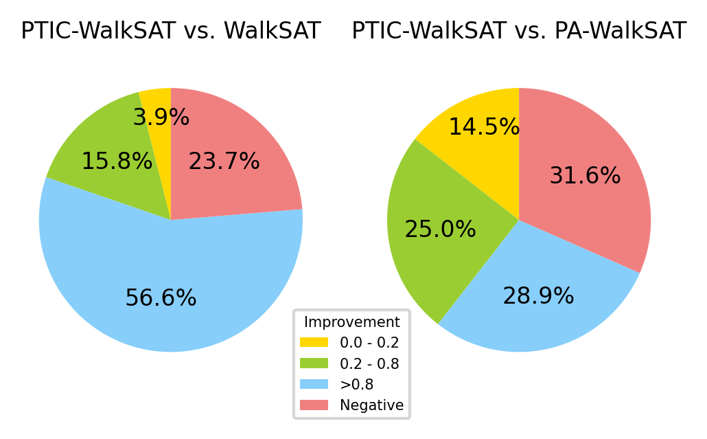
Figure 5: Charts showing the percentage of instances that fall into each improvement range

IV.4 A Per-Instance Perspective

In order to provide a full per-instance view, correlation plots are presented in Fig. 6. The y-axis shows the ITS values of the PTIC-WalkSAT algorithm while the x-axis shows that of the baselines. A point on a figure represents a problem instance; thus, there are 76 points in total. The diagonal line distinguishes where the baseline performs better (shown in the upper triangular region) and where the PTIC-WalkSAT algorithm performs better (lower region), annotated with the total number of instances in each region.

The figure on the left provides a comparison between the WalkSAT heuristic and the PTIC-WalkSAT algorithm, where, for 58 of the 76 instances, the PTIC-WalkSAT algorithm outperforms the WalkSAT heuristic. In addition, most of the points in the upper region are near the diagonal line, indicating that the WalkSAT heuristic’s advantage over the PTIC-WalkSAT algorithm is not substantial even in the case of those favourable instances. The figure on the right shows the PA-WalkSAT and PTIC-WalkSAT algorithms, a slightly closer comparison. The PTIC-WalkSAT algorithm performs better for 52 out of the 76 instances.

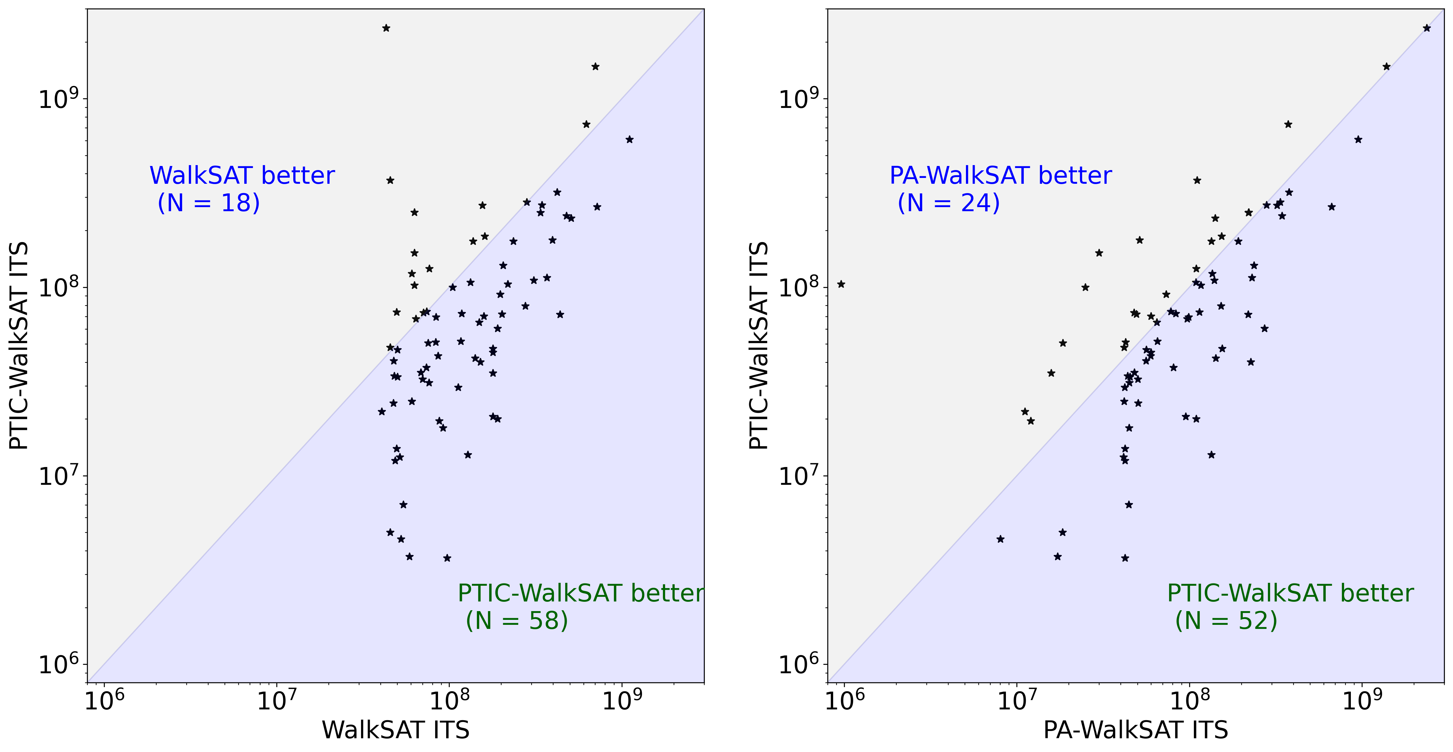
Figure 6: Correlation plots for ITS values between the PTIC-WalkSAT algorithm and the baselines

V Discussion

Our work provides strong evidence that the PTIC framework can help build faster and more-efficient binary optimization solvers. Moreover, we estimate the energy consumption overhead for two candidate IMC hardware architectures and show that, in both cases, it would amount to a less than 1% increase in energy consumption, making the framework an excellent fit for novel IMC solvers.

The computational results show that the PTIC framework, when combined with the WalkSAT heuristic, outperforms standard and parallelized versions of the WalkSAT heuristic when measuring the ITS across all replicas. We expect that a hardware implementation of the PTIC-WalkSAT algorithm will have a faster time-to-solution and require less energy than standard and parallelized versions of the WalkSAT heuristic, while being less complicated to implement than other cooperative heuristics.

The PTIC-WalkSAT algorithm has fewer total ITS than a single WalkSAT heuristic replica and a parallelized version of theWalkSAT heuristic for 76.3% and 68.4% of the problem instances, respectively. Both the PTIC-WalkSAT algorithm and the parallelized WalkSAT heuristic have the same number of replicas and the same distribution of random walk probabilities, raising the question of why the PTIC-WalkSAT algorithm yields better results. We believe the answer lies in the replica-exchange mechanism. As discussed in Sec. II, through the replica-exchange mechanism, high-temperature replicas have a better chance of exploring new solution basins and moving those solutions to lower temperatures so that the low-temperature replicas can efficiently converge to optimal solutions. Thus, it is not surprising that the PTIC-WalkSAT algorithm outperforms the version that does not possess the replica-exchange mechanism. For a more detailed discussion on the replica-exchange mechanism, see Sec. A1 of the appendix.

This study has some limitations. First, our study considers only replicas implementing the original WalkSAT formulations, and in the years since it was first postulated, there have been many improvements. We believe the PTIC framework can be applied to the majority of the improved heuristics, as well as to other, more general SAT heuristics, and possibly to other problems. Second, we evaluate the PTIC-WalkSAT algorithm on a limited number of instances: we choose four SAT classes that are known to produce hard instances and filter out the 82% easiest-to-solve instances. It is possible that the PTIC-WalkSAT algorithm’s ability to solve hard problem instances does not necessarily imply there will be comparable performance gains for simpler problems. However, energy and runtime costs are dominated by hard problem instances, so we believe this is the area where improvements to solvers can have the greatest impact. Third, the PTIC framework generalizes PT and does not require Metropolis–Hastings updates; because of this its system dynamics may differ from the established understanding of PT [13]. A potential future research direction would be to generalize PT-specific techniques, such as temperature-setting methods under a generalized notion of what temperature represents in each replica.

VI Conclusion

Our study has been motivated by the recent growing interest in in-memory computing (IMC) binary optimization solvers. The principal idea of the study has been to propose an algorithmic framework to parallelize almost any IMC solver for better performance while controlling the overhead involved in the hardware implementation. We were inspired by the parallel tempering (PT) method and proposed the “PT-inspired cooperative” (PTIC) framework, which essentially launches multiple replicas of an IMC solver with different noise configurations. Following a scheme similar to PT, replicas are executed in a cooperative way. We applied the framework to the IMC solver proposed in Ref. [3] to solve the SAT problems that the IMC solver struggles to handle.

By carrying out computational experiments, we have shown that the resultant PTIC-WalkSAT algorithm outperforms two baselines: the WalkSAT heuristic (a proxy for the IMC solver from Ref. [3]) and the native parallelization of the WalkSAT heuristic, or “PA-WalkSAT”. This shows the effectiveness of the PTIC framework, which we believe can be extended to other IMC solvers to achieve better performance.

Appendix

A1 Internal Dynamics of the PTIC-WalkSAT Algorithm

For a parallel tempering algorithm, it is important to know how replicas traverse different temperatures [17]. Having a replica frequently switch between two temperatures is not a desirable situation, as it would imply the replica exploring highly similar configuration spaces associated with the two temperatures. On the other hand, having a replica rarely travel between two temperatures is not desirable, either, as it would undermine the advantage of overcoming local energy traps by replica exchanges.

To showcase the per-replica behaviours, we use the problem instance “7SAT-60” as an example. Among 100 repeats of solving the chosen problem instance, we select the result from one of the repeats that successfully found the solution.

Figure A1 illustrates the traversal history across a full range of temperatures of a replica (“Replica 4”) able to find the solution in the end. The figure assists in verifying that all the temperatures contribute to the path towards the solution. As is evident, the replica explores the solution space using relatively low temperatures within the first few episodes. Then, after approximately 20 episodes, it jumps to the highest temperature and drops to lower temperatures a few times. Eventually, the replica remains at lower temperatures and finds the solution using the lowest temperature.

Figure A1: Replica 4 traversal history

This process shows a typical search of a successful replica. It quickly finds a good lower-energy configuration in the beginning using lower temperatures; to escape from local minima, it jumps to higher temperatures to explore a much larger configuration space; once it finds a promising space in terms of its search for the global minimum, it performs a more refined search within the space and eventually the replica finds the lowest-energy configuration.

Aside from studying the traversal history of replicas, it can also be of benefit to learn how the energy evolves over the episodes for each replica, the main purpose of which is to verify whether replica exchanges carry replicas towards different energy landscapes.

Figure A2 shows the per-replica energy history for seven replicas. The colour scheme reflects the temperature at which a replica is executed during an episode.

Figure A2: Per-replica energy history for seven replicas

It is insightful to compare the energy history of Replica 5 with that of Replica 4. Replica 5, which operates at lower temperatures, remains at lower energy levels throughout the process. In contrast, Replica 4 alternates between the highest and lowest temperatures, covering a broader range of energy levels. This highlights the advantages of exploring the search space at higher temperatures, as Replica 5 ultimately fails in finding a solution. The importance of utilizing all temperature levels becomes even clearer when examining the 100 repeats conducted for this problem instance. Figure A3 shows a histogram of the number of temperatures traversed by the successful replicas over the 100 repeats. It is evident that most of the successful repeats need to traverse all the temperatures before finding a solution.

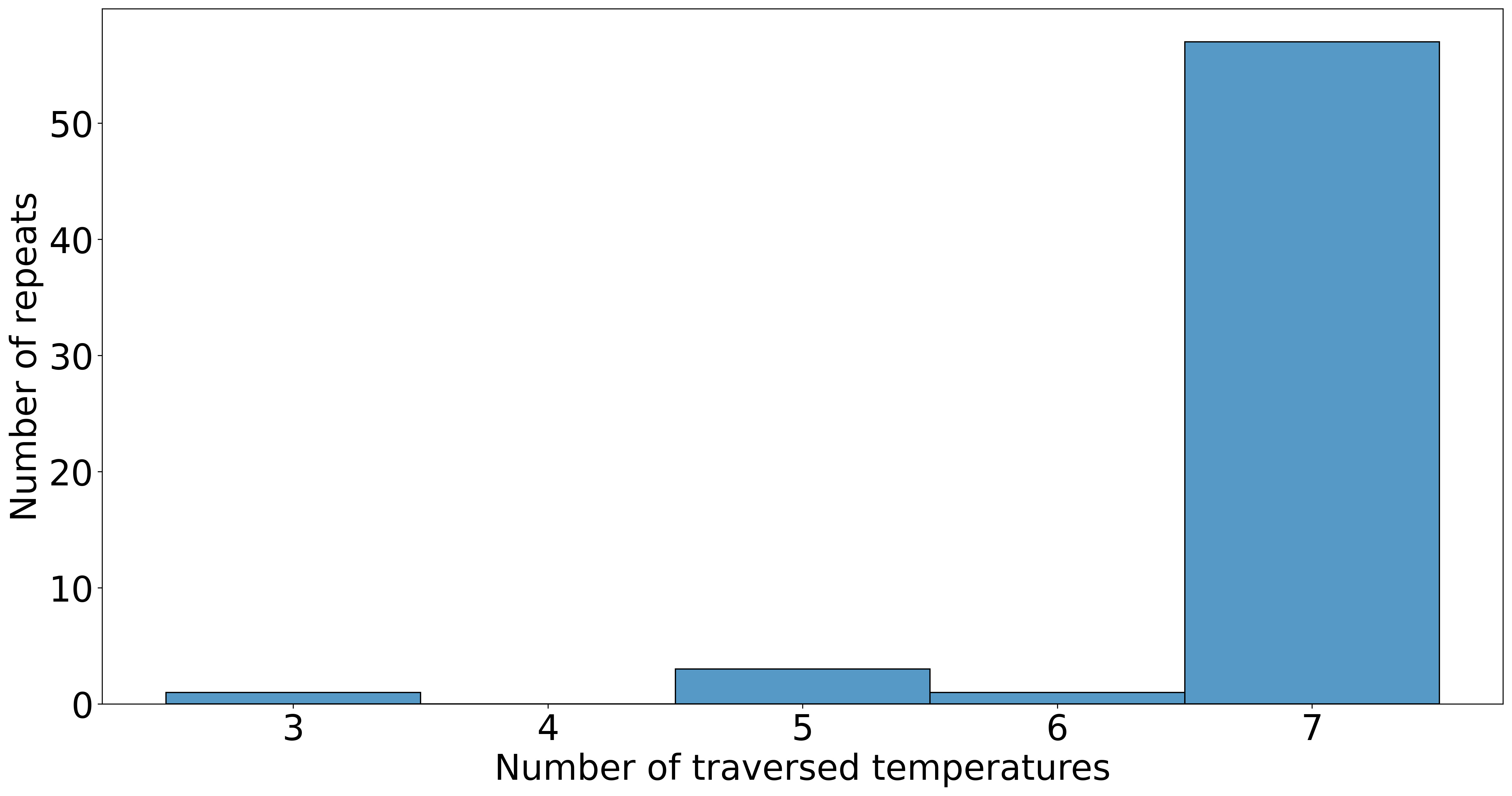
Figure A3: Histogram of the number of traversed temperatures across 100 repeats

A2 The Temperature Scheduling Algorithm

Algorithm A1  The Temperature Scheduling Algorithm

1:Given $\mathcal{T}=\{T_{1},T_{2},\ldots,T_{\kappa}\}$;

2:Initialize a scalar $v$ to a very large number;

3:while True do

4:     Get the empirical replica-exchange probabilities $\mathcal{U}=\{u_{1},u_{2},\ldots,u_{\kappa-1}\}$ by performing the PTIC-WalkSAT algorithm with the schedule $\mathcal{T}$, $Q=6720$, and for $100$ episodes (the upper limit);

5:     Calculate the variance of $\mathcal{U}$ as $\mathrm{var}(\mathcal{U})$;

6:     if $\mathrm{var}(\mathcal{U})>v$ then

7:         Break;

8:     else

9:         $v=\mathrm{var}(\mathcal{U})$;

10:         Identify the position $k=\operatorname*{arg\,min}_{i=1,2,\ldots,\kappa-1}u_{i}$;

11:         Update either $u_{k}$ or $u_{k+1}$ depending on certain conditions;

12:     end if

13:end while

14:return $\mathcal{T}$

At line 11 of Algorithm A1, the conditions are as follows.

• When $u_{k}$ is $u_{1}$, then we can update only $u_{k+1}$ by $u_{k+1}=\frac{u_{k}+u_{k+1}}{2}$

• When $u_{k+1}$ is $u_{\kappa}$, then we can update only $u_{k}$ by $u_{k}=\frac{u_{k}+u_{k+1}}{2}$

A3 The Full Benchmarking Results

Table A1: Summary of the full benchmarking results

Instance name	Group	WalkSAT ITS	PA-WalkSAT ITS	PTIC-WalkSAT ITS
4SAT-70	Group-02	52498368.25	4614330.53	8023811.83
6SAT-10	Group-03	70183652.79	32476229.17	50314177.03
6SAT-100	Group-03	179240257.57	35080937.29	15828065.64
6SAT-15	Group-03	205573667.39	130224516.23	236288236.71
6SAT-17	Group-03	47693913.75	40638183.01	56053854.71
6SAT-25	Group-03	50216849.13	33463375.83	45162860.47
6SAT-27	Group-03	50204167.71	46579216.56	56373415.42
6SAT-35	Group-03	128351410.80	12936867.81	133870448.15
6SAT-40	Group-03	62742038.51	102241114.23	116625350.79
6SAT-41	Group-03	76718107.44	125641254.54	109471780.25
6SAT-43	Group-03	149391786.81	65064251.24	64775610.15
6SAT-47	Group-03	54181803.11	7037766.09	44567960.27
6SAT-66	Group-03	60744819.87	24766425.33	41913815.66
6SAT-69	Group-03	64035469.68	68052300.60	97033242.73
6SAT-7	Group-03	344421627.00	272344173.31	279791927.85
6SAT-70	Group-03	132506224.84	106233195.27	109132487.87
6SAT-72	Group-03	76426219.99	31199004.78	44919194.82
6SAT-75	Group-03	70999823.30	73196359.52	47709872.26
6SAT-78	Group-03	40584223.81	21892300.46	11122812.76
6SAT-80	Group-03	73861994.28	74173244.49	78082158.24
6SAT-82	Group-03	202348651.27	72004378.67	49251355.52
6SAT-84	Group-03	87435080.42	19552962.13	12026606.17
6SAT-86	Group-03	367996886.23	112218872.36	230426478.97
6SAT-88	Group-03	97027844.76	3657037.80	42354230.73
6SAT-90	Group-03	75439623.90	50494719.43	18496484.54
6SAT-91	Group-03	73817441.14	37480709.70	80828243.44
6SAT-97	Group-03	62806138.30	249463054.07	221070553.08
7SAT-1	Group-04	281412199.08	282907577.80	335867906.72
7SAT-12	Group-04	179012417.17	45162352.93	59811726.96
7SAT-13	Group-04	49638132.97	13939178.48	42288898.46
7SAT-14	Group-04	151594124.09	40106344.57	227150613.24
7SAT-16	Group-04	45475886.37	368647610.19	110827037.39
7SAT-18	Group-04	308568411.99	108810848.94	139404726.41
7SAT-2	Group-04	235560377.14	174997756.76	134269252.20
7SAT-20	Group-04	1108865460.42	607883101.88	951429889.24
7SAT-3	Group-04	477065590.13	239223049.91	344388716.23
7SAT-33	Group-04	275955417.09	79588000.80	152311531.93
7SAT-37	Group-04	717940941.10	266927330.05	666762924.59
7SAT-39	Group-04	155814931.53	272040319.10	321968806.25
7SAT-4	Group-04	179054018.52	47218033.91	154638345.29
7SAT-41	Group-04	47482615.60	24297810.05	50517712.67
7SAT-43	Group-04	141489380.83	42049793.82	142006033.64
7SAT-45	Group-04	158946954.46	70051171.94	59952780.90
7SAT-46	Group-04	68448463.00	35235678.75	47978074.31
7SAT-47	Group-04	47958296.36	33774706.20	43840957.23
7SAT-49	Group-04	179156335.46	20624170.55	95149974.30
7SAT-51	Group-04	60574300.21	117999703.46	135765496.79
7SAT-52	Group-04	86132634.09	43175881.94	59681818.14
7SAT-56	Group-04	117884147.62	72383760.12	83318043.94
7SAT-59	Group-04	45487540.88	47899890.70	41916515.17
7SAT-60	Group-04	437801556.00	71769436.92	219256151.11
7SAT-61	Group-04	702023783.25	1479053372.21	1386781737.15
7SAT-62	Group-04	83417133.96	51074056.16	42729622.21
7SAT-67	Group-04	396117843.09	177903106.91	51355646.44
7SAT-68	Group-04	83894968.74	69491244.36	99133854.92
7SAT-70	Group-04	104636104.60	99698045.82	24954542.41
7SAT-71	Group-04	112776555.96	29428677.53	42163703.62
7SAT-73	Group-04	622949698.79	731721033.16	373292200.00
7SAT-74	Group-04	49613236.36	73635786.83	114264285.84
7SAT-75	Group-04	190795934.33	19993952.87	109369404.23
7SAT-79	Group-04	137588389.42	175596777.74	192105983.39
7SAT-8	Group-04	116546515.81	51723910.42	65186241.72
7SAT-80	Group-04	337440248.98	248454191.54	219825438.60
7SAT-81	Group-04	62853920.93	152179641.28	29938949.49
7SAT-82	Group-04	507762953.54	232346297.99	141047484.77
7SAT-83	Group-04	48610948.76	12027591.00	42278446.71
7SAT-84	Group-04	92158542.38	17936676.56	44751299.08
7SAT-86	Group-04	160502618.61	186496869.08	153440048.48
7SAT-9	Group-04	422003029.16	319480074.59	378087725.74
7SAT-92	Group-04	51664429.59	12551384.53	41495215.71
7SAT-95	Group-04	218381481.92	103945837.37	958956.58
7SAT-96	Group-04	197508070.80	91569133.83	73224459.91
7SAT-98	Group-04	190843039.33	60402940.22	272260147.85
prime-015	Group-01	58828837.11	3732275.60	17208428.39
prime-016	Group-01	45502435.69	5006078.42	18371874.36
prime-017	Group-01	43039540.53	2371670540.66	2373136449.37

References

- [1] M. N. Bojnordi and E. Ipek, “Memristive Boltzmann machine: A hardware accelerator for combinatorial optimization and deep learning,” in 2016 IEEE International Symposium on High Performance Computer Architecture (HPCA), pp. 1–13 (IEEE, 2016).
- [2] F. Cai, S. Kumar, T. Van Vaerenbergh, R. Liu, C. Li, S. Yu, Q. Xia, J. J. Yang, R. Beausoleil, W. Lu, et al., “Harnessing intrinsic noise in memristor Hopfield neural networks for combinatorial optimization,” arXiv:1903.11194 (2019).
- [3] G. Pedretti, F. Böhm, M. Hizzani, T. Bhattacharya, P. Bruel, J. Moon, S. Serebryakov, D. Strukov, J. Strachan, J. Ignowski, et al., “Zeroth and higher-order logic with content addressable memories,” in 2023 International Electron Devices Meeting (IEDM), pp. 1–4 (IEEE, 2023).
- [4] T. Bhattacharya, G. H. Hutchinson, G. Pedretti, X. Sheng, J. Ignowski, T. Van Vaerenbergh, R. Beausoleil, J. P. Strachan, and D. B. Strukov, “Computing High-Degree Polynomial Gradients in Memory,” arXiv:2401.16204 (2024).
- [5] A. Sharma, M. Burns, A. Hahn, and M. Huang, “Augmenting an electronic Ising machine to effectively solve Boolean satisfiability,” Scientific Reports 13, 22858 (2023).
- [6] T. G. Crainic and M. Toulouse, Parallel meta-heuristics (Springer, 2010).
- [7] T. Harada and E. Alba, “Parallel genetic algorithms: a useful survey,” ACM Computing Surveys (CSUR) 53, 1 (2020).
- [8] A. Silva, L. C. Coelho, and M. Darvish, “Quadratic assignment problem variants: A survey and an effective parallel memetic iterated tabu search,” European Journal of Operational Research 292, 1066 (2021).
- [9] A. McDonald et al., “Parallel WalkSAT with clause learning,” Data analysis project papers (2009).
- [10] T. G. Crainic, M. Gendreau, P. Hansen, and N. Mladenović, “Cooperative parallel variable neighborhood search for the p-median,” Journal of heuristics 10, 293 (2004).
- [11] O. Polat, “A parallel variable neighborhood search for the vehicle routing problem with divisible deliveries and pickups,” Computers & Operations Research 85, 71 (2017).
- [12] P. Jarvis and A. Arbelaez, “Cooperative parallel SAT local search with path relinking,” in Evolutionary Computation in Combinatorial Optimization: 20th European Conference, EvoCOP 2020, Held as Part of EvoStar 2020, Seville, Spain, April 15–17, 2020, Proceedings 20, pp. 83–98 (Springer, 2020).
- [13] K. Hukushima and K. Nemoto, “Exchange Monte Carlo method and application to spin glass simulations,” Journal of the Physical Society of Japan 65, 1604 (1996).
- [14] C. J. Geyer, “Monte Carlo Maximum Likelihood for Dependent Data,” in E. M. Keramidas (ed.), 23rd Symposium on the Interface, p. 156 (Interface Foundation, Fairfax Station, VA, 1991).
- [15] J. Moreno, H. G. Katzgraber, and A. K. Hartmann, “Finding low-temperature states with parallel tempering, simulated annealing and simple Monte Carlo,” International Journal of Modern Physics C 14, 285 (2003).
- [16] Z. Zhu, C. Fang, and H. G. Katzgraber, “borealis – A generalized global update algorithm for Boolean optimization problems,” arXiv:1605.09399 (2016).
- [17] D. J. Earl and M. W. Deem, “Parallel tempering: Theory, applications, and new perspectives,” Physical Chemistry Chemical Physics 7, 3910 (2005).
- [18] C. Wang, J. D. Hyman, A. Percus, and R. Caflisch, “Parallel tempering for the traveling salesman problem,” International Journal of Modern Physics C 20, 539 (2009).
- [19] M. Bagherbeik, P. Ashtari, S. F. Mousavi, K. Kanda, H. Tamura, and A. Sheikholeslami, “A permutational Boltzmann machine with parallel tempering for solving combinatorial optimization problems,” in International Conference on Parallel Problem Solving from Nature, pp. 317–331 (Springer, 2020).
- [20] A. Almeida, J. d. C. Lima, and M. A. Carvalho, “Revisiting the Parallel Tempering Algorithm: High-Performance Computing and Applications in Operations Research,” Available at SSRN 4756904 (2024).
- [21] M. Kim, S. Mandrà, D. Venturelli, and K. Jamieson, “Physics-inspired heuristics for soft MIMO detection in 5G new radio and beyond,” in Proceedings of the 27th Annual International Conference on Mobile Computing and Networking, pp. 42–55 (2021).
- [22] S. A. Cook, “The complexity of theorem-proving procedures,” in Proceedings of the Third Annual ACM Symposium on Theory of Computing, STOC ’71, p. 151 (Association for Computing Machinery New York NY United States, 1971).
- [23] D. S. Johnson, “Approximation algorithms for combinatorial problems,” in Proceedings of the fifth annual ACM symposium on Theory of computing, pp. 38–49 (1973).
- [24] I. Mironov and L. Zhang, “Applications of SAT solvers to cryptanalysis of hash functions,” in Theory and Applications of Satisfiability Testing-SAT 2006: 9th International Conference, Seattle, WA, USA, August 12-15, 2006. Proceedings 9, pp. 102–115 (Springer, 2006).
- [25] D. Brand, “Verification of large synthesized designs,” in Proceedings of 1993 International Conference on Computer Aided Design (ICCAD), pp. 534–537 (IEEE, 1993).
- [26] C. Castellini, E. Giunchiglia, and A. Tacchella, “SAT-based planning in complex domains: Concurrency, constraints and nondeterminism,” Artificial Intelligence 147, 85 (2003).
- [27] D. E. Knuth, The art of computer programming, Volume 4, Fascicle 6: Satisfiability (Addison-Wesley Professional, 2015).
- [28] C. Shim, J. Bae, and B. Kim, “30.3 VIP-Sat: A Boolean Satisfiability Solver Featuring 5 12 Variable In-Memory Processing Elements with 98% Solvability for 50-Variables 218-Clauses 3-SAT Problems,” in 2024 IEEE International Solid-State Circuits Conference (ISSCC), vol. 67, pp. 486–488 (IEEE, 2024).
- [29] S. Xie, M. Yang, S. A. Lanham, Y. Wang, M. Wang, S. Oruganti, and J. P. Kulkarni, “29.2 Snap-SAT: A One-Shot Energy-Performance-Aware All-Digital Compute-in-Memory Solver for Large-Scale Hard Boolean Satisfiability Problems,” in 2023 IEEE International Solid-State Circuits Conference (ISSCC), pp. 420–422 (IEEE, 2023).
- [30] B. Selman, H. A. Kautz, B. Cohen, et al., “Local search strategies for satisfiability testing.” Cliques, coloring, and satisfiability 26, 521 (1993).
- [31] H. Kautz, “WalkSAT,” https://gitlab.com/HenryKautz/Walksat.
- [32] N. Metropolis, A. W. Rosenbluth, M. N. Rosenbluth, A. H. Teller, and E. Teller, “Equation of state calculations by fast computing machines,” The journal of chemical physics 21, 1087 (1953).
- [33] W. K. Hastings, “Monte Carlo sampling methods using Markov chains and their applications,” Biometrika 57, 97 (1970).
- [34] M. Hizzani, A. Heittmann, G. Hutchinson, D. Dobrynin, T. Van Vaerenbergh, T. Bhattacharya, A. Renaudineau, D. Strukov, and J. P. Strachan, “Memristor-based hardware and algorithms for higher-order Hopfield optimization solver outperforming quadratic Ising machines,” in 2024 IEEE International Symposium on Circuits and Systems (ISCAS), pp. 1–5 (IEEE, 2024).
- [35] B. Murmann, “ADC Performance Survey 1997–2024,” https://github.com/bmurmann/ADC-survey.
- [36] A. Ankit, I. E. Hajj, S. R. Chalamalasetti, G. Ndu, M. Foltin, R. S. Williams, P. Faraboschi, W.-M. W. Hwu, J. P. Strachan, K. Roy, et al., “PUMA: A programmable ultra-efficient memristor-based accelerator for machine learning inference,” in Proceedings of the twenty-fourth international conference on architectural support for programming languages and operating systems, pp. 715–731 (2019).
- [37] J. Bebel, “Harder SAT Instances from Factoring with Karatsuba and Espresso,” in M. J. Heule, M. Järvisalo, and M. Suda (eds.), Proceedings of SAT Race 2019: Solver and Benchmark Descriptions, pp. 47–48 (Department of Computer Science, University of Helsinki, 2019).
- [38] F. Krzakala, M. Mézard, and L. Zdeborová, “Reweighted belief propagation and quiet planting for random k-SAT,” Journal on Satisfiability, Boolean Modeling and Computation 8, 149 (2012).
- [39] S. Mertens, M. Mézard, and R. Zecchina, “Threshold values of random K-SAT from the cavity method,” Random Structures & Algorithms 28, 340 (2006).
- [40] M. Aramon, G. Rosenberg, E. Valiante, T. Miyazawa, H. Tamura, and H. G. Katzgraber, “Physics-inspired optimization for quadratic unconstrained problems using a digital annealer,” Frontiers in Physics 7, 48 (2019).
- [41] T. Akiba, S. Sano, T. Yanase, T. Ohta, and M. Koyama, “Optuna: A next-generation hyperparameter optimization framework,” in Proceedings of the 25th ACM SIGKDD international conference on knowledge discovery & data mining, pp. 2623–2631 (2019).
- [42] I. Rozada, M. Aramon, J. Machta, and H. G. Katzgraber, “Effects of setting temperatures in the parallel tempering Monte Carlo algorithm,” Physical Review E 100, 043311 (2019).
- [43] K. Hukushima, “Domain-wall free energy of spin-glass models: Numerical method and boundary conditions,” Physical Review E 60, 3606 (1999).
- [44] D. A. Kofke, “On the acceptance probability of replica-exchange Monte Carlo trials,” The Journal of chemical physics 117, 6911 (2002).