Robust optimal design of large-scale Bayesian nonlinear inverse problems

Abstract

We consider robust optimal experimental design (ROED) for nonlinear Bayesian inverse problems governed by partial differential equations (PDEs). An optimal design is one that maximizes some utility quantifying the quality of the solution of an inverse problem. However, the optimal design is dependent on elements of the inverse problem such as the simulation model, the prior, or the measurement error model. ROED aims to produce an optimal design that is aware of the additional uncertainties encoded in the inverse problem and remains optimal even after variations in them. We follow a worst-case scenario approach to develop a new framework for robust optimal design of nonlinear Bayesian inverse problems. The proposed framework a) is scalable and designed for infinite-dimensional Bayesian nonlinear inverse problems constrained by PDEs; b) develops efficient approximations of the utility, namely, the expected information gain; c) employs eigenvalue sensitivity techniques to develop analytical forms and efficient evaluation methods of the gradient of the utility with respect to the uncertainties we wish to be robust against; and d) employs a probabilistic optimization paradigm that properly defines and efficiently solves the resulting combinatorial max-min optimization problem. The effectiveness of the proposed approach is illustrated for optimal sensor placement problem in an inverse problem governed by an elliptic PDE.

65C20, 35R30, 62K05, 62F15

1 Introduction

The Bayesian approach to inverse problems is ubiquitous in the uncertainty quantification and computational science communities. The quality of the solution to such inverse problems is highly dependent on the design of the data collection mechanism. However, data acquisition is often expensive. This can put severe limits on the amount of data that can be collected. Thus, it is important to allocate the limited data collection resources optimally. This can be formulated as an optimal experimental design (OED) problem [6, 15, 19, 44, 23]. An OED problem seeks to identify experiments that optimize the statistical quality of the solution to the inverse problem. While OED may be applied to a variety of observation configurations, in this work we focus on optimal sensor placement. Fast and accurate OED methods for optimal design of inverse problems governed by partial differential equations (PDEs) has been a topic of interest over the pass couple of decades; see [1] for a review of the literature on such methods.

Inverse problems arising from complex engineering applications typically have misspecifications and/or uncertainties in hyperparameters defining the inverse problem. These hyperparameters can have a significant impact on the quality of parameter estimation. This has sparked interest in efforts such as [25, 26, 34] that consider Bayesian inversion under various modeling uncertainties. See also [18, 21, 41], which consider analyzing the sensitivity of the solution of a Bayesian inverse problem to uncertain parameters in the prior, likelihood, and governing equations. The uncertainty in the hyperparameters, especially the most influential ones, needs to be accounted for in the OED problem as well. This can be addressed by a robust OED (ROED) approach. This work develops a novel ROED approach for nonlinear Bayesian inverse problems governed by PDEs with infinite-dimensional parameters. For consistency, hereafter, we will use the term uncertain parameter for any uncertain element of the inverse problem considered in an ROED framework. On the other hand, we use the term inversion parameter for the parameter being estimated in an inverse problem.

Related Work. There have been several approaches to ROED in literature. For example, the efforts [37, 42, 43] consider finding an optimal design against a statistical average over the distribution of the uncertain parameters. This is also related to the approach in [27], which formulates the OED problem for parameterized linear inverse problems as an optimization problem under uncertainty problem. Other related efforts include [3, 4, 12]. In this work, we seek to guard against the worst-case scenarios, and thus adopt Wald’s “max-min” model [46], which seeks a design that is optimal against a lower bound of the objective over admissible values of the uncertain parameter. A generic statement of the ROED problems under study is as follows:

Problem 1.1.

roed Consider the set of candidate sensor locations $\mathcal{S}=\{s_{1},s_{2},\ldots,s_{{\rm N_{d}}}\}$, and let ${\rm N_{b}}\ll{\rm N_{d}}$ be the budget constraint on the number of sensors. Let $\bm{\xi}\in\{0,1\}^{{\rm N_{d}}}$ be a binary encoding of the observational configuration such that $\xi_{i}$ determines whether $s_{i}$ is active, and let $\bm{\theta}\in\Theta$ be the uncertain parameter. The ROED problem is defined as the optimization problem

(1a) $$\max_{\bm{\xi}\in\mathcal{S}({\rm N_{b}})}\min_{\bm{\theta}\in\Theta}\,\mathcal{U}(\bm{\xi},\bm{\theta})\,,$$

where

(1b) $$\mathcal{S}({\rm N_{b}})=\bigg{\{}\bm{\xi}\in\{0,1\}^{{\rm N_{d}}}\mathrel{\mathop{\ordinarycolon}}\sum_{i=1}^{{\rm N_{d}}}\xi_{i}={\rm N_{b}}\bigg{\}}\,,$$

and the utility (objective) $\mathcal{U}$ is chosen to quantify the quality of the design.

While conservative ROED approaches has been studied in the past [13, 22, 37, 39], most approaches were not designed to scale to large-scale inverse problems or large binary design spaces. The work [9] recasts the conservative (worst-case-scenario) max-min formulation of the ROED problem into a probabilistic optimization framework. A desirable aspect of this development is in providing a scalable computational framework. The approach proposed in [9], however, focuses on ROED for linear inverse problems. In this article, we extend the probabilistic ROED approach in [9] to nonlinear Bayesian inverse problems.

Our approach and contributions. For the utility $\mathcal{U}$, we employ the expected information gain (EIG). In this context, information gain is defined by the Kullback–Leibler divergence [28] of the posterior from the prior,

(2a) $$D_{\rm KL}(\mu_{\rm post}^{\mathbf{y}}\|\mu_{\rm pr})\mathrel{\mathop{\ordinarycolon}}=\int\log\left(\derivative{\mu_{\rm post}^{\mathbf{y}}}{\mu_{\rm pr}}\right)\differential{\mu_{\rm post}^{\mathbf{y}}}.$$

And the EIG is defined by

(2b) $$\overline{D_{\rm KL}}\mathrel{\mathop{\ordinarycolon}}=\mathbb{E}_{\mathbf{y}}\left[D_{\rm KL}(\mu_{\rm post}^{\mathbf{y}}||\mu_{\rm pr})\right]\,.$$

Here, $\mu_{\rm pr}$ is the prior distribution law of the inversion parameter and $\mu_{\rm post}^{\mathbf{y}}$ is the posterior measure. This utility (2) admits a computationally tractable closed-form expression in the case of Bayesian linear inverse problems [2]. However, there is no such expression in the case of nonlinear inverse problems.

In this work, we present an approximation framework for estimating the utility function (2) for infinite-dimensional Bayesian nonlinear inverse problems governed by PDEs. This framework enables efficient evaluation of the objective $\mathcal{U}$ and its derivative with respect to the uncertain parameter which is essential for the proposed ROED approach. Our formulations of the utility function and its gradient are based on low-rank approximations and adjoint-based eigenvalue sensitivity analysis [47, 18]. To enforce the budget constraint, the method in [9] leveraged a soft-constraint by adding a penalty term to the optimization objective function. However, as pointed out in [7] this approach requires challenging tuning of the penalty parameter. Our proposed ROED approach leverages ideas presented in a newly developed probabilistic approach for budget-constrained binary optimization [7]. We summarize the novel contributions of this article as follows: we present an ROED framework for infinite-dimensional nonlinear Bayesian inverse problems by

1. developing a scalable framework for evaluation and differentiation of the EIG (2) chosen as the utility function for nonlinear ROED; and

2. developing a budget-constrained probabilistic max-min optimization framework that does not rely on penalty methods, hence eliminating the need for an expensive penalty-parameter tuning stage.

Article organization. Section 2 provides the requisite background for infinite-dimensional Bayesian inverse problems constrained by PDEs and ROED. Section 3 presents our proposed probabilistic approach for nonlinear ROED. Computational results demonstrating the effectiveness of the proposed methods are in Section 4. Concluding remarks are outlined in Section 5.

2 Preliminaries

In this section, we present the necessary mathematical background and notation for this work. We review infinite-dimensional Bayesian inference in Section 2.1 and ROED in Section 2.2.

2.1 PDE-Constrained Bayesian Inverse Problems

Consider a PDE model stated in the following implicit abstract form: given $m\in\mathscr{M}$, find $u\in\mathscr{U}$ such that

(3) $$\mathcal{A}(u,m)=0\,.$$

Here, $u$ is the state variable and $m$ is the inversion parameter. These variables are assumed to belong to Hilbert spaces $\mathscr{U}$ and $\mathscr{M}$, respectively.

In this formulation, $\mathcal{A}\mathrel{\mathop{\ordinarycolon}}\mathscr{U}\times\mathscr{M}\to\mathscr{V}^{\prime}$ is a representation of the strong form of a PDE. Here, $\mathscr{V}^{\prime}$ is the dual of an appropriately chosen Hilbert space $\mathscr{V}$, which in the present setting is typically called the test function space. The weak form corresponding to (3) is formulated as follows: Given $m\in\mathscr{M}$, find $u\in\mathscr{U}$ such that

(4) $$a(u,m,p)\coloneqq\left\langle p,\mathcal{A}(u,m)\right\rangle=0\quad\forall\,p\in\mathscr{V},$$

where $\left\langle\cdot,\cdot\right\rangle\mathrel{\mathop{\ordinarycolon}}\mathscr{V}\times\mathscr{V}^{\prime}\to\mathbb{R}$ is the dual pairing between $\mathscr{V}$ and $\mathscr{V}^{\prime}$. Note that $a$ is linear in the test variable $p$, but it may be nonlinear in both $u$ and $m$, respectively.

We assume a data model of the following form:

(5) $$\mathbf{y}=\bm{\mathcal{Q}}(u)+\bm{\eta},$$

where $u$ satisfies (4), $\bm{\mathcal{Q}}\mathrel{\mathop{\ordinarycolon}}\mathscr{U}\to\mathbb{R}^{d}$ is an observation operator that maps the state variable $u$ to the data $\mathbf{y}\in\mathscr{Y}$ at ${\rm N_{d}}$ observation points. For simplicity, we assume that each sensor observes only one prognostic variable, and thus the dimension of the observation vector is equal to the number of sensors. This simplification, however, does not limit the formulation nor the approaches presented in this work. Finally, we assume $\bm{\eta}\sim\mathcal{N}(\mathbf{0},\mathbf{{\Gamma}}_{\rm n})$ in (5).

We also define the parameter to observable map

(6) $$\bm{\mathcal{F}}(m)=\bm{\mathcal{Q}}(u(m))\,,$$

which maps the inversion parameter $m$ onto the observation space. Henceforth, we assume that $\bm{\mathcal{F}}$ is Fréchet differentiable with respect to $m$. To formulate the posterior law of the inversion parameter, we assume a Gaussian prior measure $\mu_{\rm pr}=\mathcal{N}(m_{\rm pr},\mathcal{C}_{\rm pr})$ with $\mathcal{C}_{\rm pr}$ a strictly positive self-adjoint operator of trace class; see, e.g., [40] for details. Here, $m_{\rm pr}\in\mathcal{E}$ where $\mathcal{E}=\operatorname{range}(\mathcal{C}_{\rm pr}^{1/2})$ is a Cameron-Martin space, induced by the prior measure, and is equipped with the following inner product

(7) $$\left\langle x,y\right\rangle_{\mathcal{C}_{\rm pr}^{-1}}=\left\langle\mathcal{C}_{\rm pr}^{-1/2}x,\mathcal{C}_{\rm pr}^{-1/2}y\right\rangle_{\!\!\mathscr{M}},\quad\forall x,y\in\mathcal{E}\,.$$

These assumptions on the data model and prior, along with Bayes’ rule, define a posterior measure $\mu_{\rm post}^{\mathbf{y}}$ on $\mathscr{M}$ given by the Radon–Nikodym derivative

(8) $$\derivative{\mu_{\rm post}^{\mathbf{y}}}{\mu_{\rm pr}}\propto\pi_{\rm like}(\mathbf{y}|m).$$

Note that under the additive Gaussian noise model (5), the likelihood $\pi_{\rm like}$ satisfies

(9) $$\pi_{\rm like}(\mathbf{y}|m)\propto\exp\left(-\frac{1}{2}\norm{\mathbf{y}-\bm{\mathcal{F}}(m)}_{\mathbf{{\Gamma}}_{\rm n}^{-1}}^{2}\right),$$

where we have used the weighted norm $\left\|{\mathbf{x}}\right\|^{2}_{\mathbf{{\Gamma}}_{\rm n}^{-1}}\mathrel{\mathop{\ordinarycolon}}=\mathbf{x}^{\mkern-1.5mu\mathsf{T}}\mathbf{{\Gamma}}_{\rm n}^{-1}\mathbf{x}$. If the parameter-to-observable map $\bm{\mathcal{F}}$ is linear, then it can be demonstrated [40] that the posterior measure is Gaussian $\mu_{\rm post}^{\mathbf{y}}=\mathcal{N}(m_{\rm post},\mathcal{C}_{\rm post})$ with

(10) $$\mathcal{C}_{\rm post}=\left(\mathcal{C}_{\rm pr}^{-1}+\bm{\mathcal{F}}^{*}\mathbf{{\Gamma}}_{\rm n}^{-1}\bm{\mathcal{F}}\right)^{-1}\,;\qquad m_{\rm post}=\mathcal{C}_{\rm post}\big{(}\bm{\mathcal{F}}^{*}\mathbf{{\Gamma}}_{\rm n}^{-1}\mathbf{y}+\mathcal{C}_{\rm pr}^{-1}m_{\rm pr}\big{)}\,,$$

$\bm{\mathcal{F}}^{*}$ is the adjoint of $\bm{\mathcal{F}}$. In this work, however, we consider the case where the parameter-to-observable map $\bm{\mathcal{F}}$ is nonlinear. Hence, the posterior measure is generally not available in closed form. Nevertheless, there are several practical approaches to analyze the posterior measure and estimate the inversion parameter. One such tool is to consider the maximum a posteriori (MAP) point, which is the minimizer of the functional

(11) $$\Phi(m)\mathrel{\mathop{\ordinarycolon}}=\frac{1}{2}\norm{\mathbf{y}-\bm{\mathcal{F}}(m)}_{\mathbf{{\Gamma}}_{\rm n}^{-1}}^{2}+\frac{1}{2}\norm{m-m_{\rm pr}}_{\mathcal{C}_{\rm pr}^{-1}}^{2}\,,$$

over the Cameron-Martin space $\mathcal{E}$. The MAP provides a point estimate of the unknown inversion parameter. It is also possible to obtain a local Gaussian approximation of the posterior, known as the Laplace approximation. This is discussed next.

The Laplace Approximation. A commonly used tool in large-scale nonlinear Bayesian inverse problem is the Laplace approximation approach [40, 14], which aims to approximate the posterior by an appropriate Gaussian distribution. In the present work, we utilize this approximation to obtain an approximation of the EIG. The Laplace approximation $\hat{\mu}_{\rm post}^{\mathbf{y}}=\mathcal{N}(m_{\rm post},\mathcal{C}_{\rm post})$ has mean $m_{\rm post}$ given by the maximum a posteriori (MAP) point

(12a) $$m_{\rm post}\mathrel{\mathop{\ordinarycolon}}=\operatorname*{arg\,min}_{m\in\mathcal{E}}\Phi(m)$$

where $$\Phi(m) \mathcal{C}_{\rm post}$$ is given by (11), and the covariance is given by the inverse Hessian of (11) evaluated at the MAP point

(12b) $$\mathcal{C}_{\rm post}^{-1}=\mathcal{H}_{\rm m}(m_{\rm post})+\mathcal{C}_{\rm pr}^{-1}.$$

Here, $\mathcal{H}_{\rm m}(m_{\rm post})$ is the Hessian of the data misfit term $\frac{1}{2}\|\mathbf{y}-\bm{\mathcal{F}}(m)\|_{\mathbf{{\Gamma}}_{\rm n}^{-1}}^{2}$ evaluated at $m_{\rm post}$. In practice, a commonly used approximation to this data-misfit Hessian is the Gauss–Newton approximation given by

(13) $$\mathcal{H}_{\rm m}(m_{\rm post})=\bm{\mathcal{J}}^{*}(m_{\rm post})\mathbf{{\Gamma}}_{\rm n}^{-1}\bm{\mathcal{J}}(m_{\rm post}),$$

where $\bm{\mathcal{J}}(m_{\rm post})$ is the Jacobian of $\bm{\mathcal{F}}(m)$ with respect to $m$ evaluated at $m_{\rm post}$. We employ this approximation in our work, and henceforth we use the simplified notation $\mathcal{H}_{\rm m}$ to refer to the expression in (13). We note that with the Gauss–Newton Hessian approximation (13), the Laplace approximation is equivalent to the posterior measure obtained after a linearization of the parameter-to-observable map $\bm{\mathcal{F}}$ at the MAP point $m_{\rm post}$; see e.g., [3].

Variational Tools. The gradient and the Hessian of the cost functional (11) are essential components of our proposed methods. To compute these derivatives, we rely on adjoint-based gradient computation [36], derived using a formal Lagrangian approach. Here, we outline the adjoint-based expressions for the gradient and Hessian apply. We begin by defining the Lagrangian

(14) $$\mathcal{L}(u,m,p)=\frac{1}{2}\norm{\mathbf{y}-\bm{\mathcal{Q}}u}_{\mathbf{{\Gamma}}_{\rm n}^{-1}}^{2}+\frac{1}{2}\norm{m-m_{\rm pr}}_{\mathcal{C}_{\rm pr}^{-1}}^{2}+a(u,m,p)\,.$$

In this context, $p$ is called the adjoint variable. The gradient of (11) is given by the variation of this Lagrangian with respect to $m$, assuming the variations of $\mathcal{L}$ with respect to $u$ and $p$ vanish. Namely,

(15a) $$\mathcal{G}(m)(\tilde{m})=\left\langle\tilde{m},m-m_{\rm pr}\right\rangle_{\mathcal{C}_{\rm pr}^{-1}}+\left\langle\tilde{m},a_{m}(u,m,p)\right\rangle\,,$$

where $$u p$$ and satisfy

(15b) $$\left\langle\tilde{p},a_{p}(u,m,p)\right\rangle =0\quad\forall\tilde{p}\in\mathscr{V}\,,$$

(15c) $$\left\langle\tilde{u},a_{u}(u,m,p)\right\rangle+\left\langle\tilde{u},\bm{\mathcal{Q}}^{*}\mathbf{{\Gamma}}_{\rm n}^{-1}(\mathbf{y}-\bm{\mathcal{Q}}u)\right\rangle =0\quad\forall\tilde{u}\in\mathscr{V}\,.$$

To compute the Hessian action of (11), we follow a Lagrange multiplier approach to differentiate through the gradient (15a) constrained by the state and adjoint equations (15b), and (15c), respectively. A detailed discussion of deriving adjoint-based Hessian apply expressions can be found in [45]. As explained later, in our proposed approach we only require the data-misfit Hessian $\mathcal{H}_{\rm m}$. To derive the adjoint-based data-misfit Hessian action we consider the meta-Lagrangian

$$\mathcal{L}^{H}(u,m,p,\hat{u},\hat{m},\hat{p})=\\ \left\langle\hat{m},a_{m}(u,m,p)\right\rangle+\left\langle\hat{p},a_{p}(u,m,p)\right\rangle+\left\langle\hat{u},a_{u}(u,m,p)\right\rangle+\left\langle\hat{u},\bm{\mathcal{Q}}^{*}\mathbf{{\Gamma}}_{\rm n}^{-1}(\mathbf{y}-\bm{\mathcal{Q}}u)\right\rangle\,.$$

Through a similar process as before, we take a variation of $\mathcal{L}^{H}$ with respect to $m$ and constrain it by letting variations of $\mathcal{L}^{H}$ with respect to $\hat{u}$ and $\hat{p}$ vanish. This yields the expression for the data-misfit Hessian action:

(16a) $$\mathcal{H}_{\rm m}(m)(\hat{m},\tilde{m})=\left\langle\tilde{m},a_{mm}(u,m,p)\hat{m}+a_{mu}(u,m,p)\hat{u}+a_{mp}(u,m,p)\hat{p}\right\rangle\,,$$

where for all $$\tilde{p}\in\mathscr{V} \tilde{u}\in\mathscr{V}$$ and ,

(16b) $$\left\langle\tilde{p},a_{pu}(u,m,p)\hat{u}\right\rangle+\left\langle\tilde{p},a_{pm}(u,m,p)\hat{m}\right\rangle =0\,,$$

(16c) $$\left\langle\tilde{u},a_{up}(u,m,p)\hat{p}+a_{uu}(u,m,p)\hat{u}+a_{um}(u,m,p)\hat{m}\right\rangle+\left\langle\tilde{u},\bm{\mathcal{Q}}^{*}\mathbf{{\Gamma}}_{\rm n}^{-1}\bm{\mathcal{Q}}\hat{u}\right\rangle =0\,.$$

Finally, the Gauss-Newton Hessian is obtained by dropping the terms involving the adjoint variable; see [11] for details. In the present setting, the Gauss-Newton data-misfit Hessian action is given by

(17a) $$\mathcal{H}(m)(\hat{m},\tilde{m})=\left\langle\tilde{m},a_{mm}(u,m,p)+a_{mu}(u,m,p)\hat{u}+a_{mp}(u,m,p)\hat{p}\right\rangle,$$

where for all $$\tilde{p}\in\mathscr{V} \tilde{u}\in\mathscr{V}$$ and ,

(17b) $$\left\langle\tilde{p},a_{pu}(u,m,p)\hat{u}\right\rangle+\left\langle\tilde{p},a_{pm}(u,m,p)\hat{m}\right\rangle =0\,,$$

(17c) $$\left\langle\tilde{u},a_{up}(u,m,p)\hat{p}\right\rangle+\left\langle\tilde{u},\bm{\mathcal{Q}}^{*}\mathbf{{\Gamma}}_{\rm n}^{-1}\bm{\mathcal{Q}}\hat{u}\right\rangle =0\,.$$

Both (15), and (17) play a central role in the computational framework presented in Section 3. Although, in this work, we focus on the setting of time-independent PDEs, much of the framework can be extended to time-dependent PDEs or other forms of governing equations as well.

2.2 Robust Optimal Experimental Design

As stated in LABEL:prob:roed, our goal is to find a robust optimal design $\bm{\xi}^{\rm opt}$ that solves the ROED optimization problem

(18) $$\max_{\bm{\xi}\in\mathcal{S}({\rm N_{b}})}\min_{\bm{\theta}\in\Theta}\,\mathcal{U}(\bm{\xi},\bm{\theta})\,,$$

where $\mathcal{U}$ is the chosen utility function. Let us contrast this with the traditional (non-robust) optimal design that solves the binary optimization problem

(19) $$\max_{\bm{\xi}\in\mathcal{S}({\rm N_{b}})}\mathcal{U}(\bm{\xi}).$$

The ROED problem (18) can be viewed as a bi-level optimization problem, with the outer optimization layer bearing resemblance to the traditional OED problem (19). Hence, solving the ROED problem is considerably more challenging than the traditional OED problem.

Some of the commonly used techniques for solving traditional OED problems are not suitable for the ROED problem. Notably, we recall that a commonly used technique for solving (19) is a relaxation approach. In this approach the design space is relaxed from a binary space $\{0,1\}^{{\rm N_{d}}}$ to a continuum $[0,1]^{{\rm N_{d}}}$. This enables the use of gradient-based optimization techniques. However, as noted in [9], a naive reformulation of (18) into this relaxed form is incorrect because

$$\operatorname*{arg\,max}_{\bm{\xi}\in\{0,1\}^{{\rm N_{d}}}}\min_{\bm{\theta}\in\Theta}\,\mathcal{U}(\bm{\xi},\bm{\theta})\not\subset\operatorname*{arg\,max}_{\bm{\xi}\in[0,1]^{{\rm N_{d}}}}\min_{\bm{\theta}\in\Theta}\,\mathcal{U}(\bm{\xi},\bm{\theta}).$$

Specifically, it was demonstrated in [9] that relaxation of the binary design in (18) results in a different optimization problem with different optimal set than the solution of (18). To overcome this challenge, [9] introduced an extension of a stochastic optimization framework [10] to the ROED setting and demonstrated that the resulting probabilistic ROED formulation is equivalent to the original binary max-min ROED optimization problem (18). LABEL:prob:old-stochastic-roed summarizes this probabilistic ROED formulation. In the present work, we consider extensions of such formulations to budget-constrained ROED for nonlinear Bayesian inverse problems.

Problem 2.1.

old-stochastic-roed Consider the set of candidate sensor locations $\mathcal{S}=\{s_{1},s_{2},\ldots,s_{{\rm N_{d}}}\}$. Let $\bm{\xi}\in\{0,1\}^{{\rm N_{d}}}$ be a binary encoding of the observational configuration such that $\xi_{i}$ determines if $s_{i}$ is active. Let $\bm{\theta}\in\Theta$ be the uncertain parameter we seek to be robust against. The probabilistic ROED approach views $\bm{\xi}$ as a random variable endowed with a multivariate Bernoulli distribution $\mathbb{P}(\bm{\xi}|\mathbf{p})$ parameterized by $\mathbf{p}\in[0,1]^{{\rm N_{d}}}$ , where $p_{i}\in[0,1]$ is the probability of activating $s_{i}$.

The probabilistic ROED problem aims to find a policy $\mathbf{p}^{\rm opt}$ that solves

(20) $$\max_{\mathbf{p}\in[0,1]^{{\rm N_{d}}}}\mathfrak{U}(\mathbf{p})\mathrel{\mathop{\ordinarycolon}}=\mathbb{E}_{\bm{\xi}\sim\mathbb{P}(\bm{\xi}|\mathbf{p})}\left[\min_{\bm{\theta}\in\Theta}\,\mathcal{U}(\bm{\xi},\bm{\theta})\right]\,.$$

Here, $\mathbb{P}(\bm{\xi}|\mathbf{p}^{\rm opt})$ yields the solution of the binary ROED problem (18).

The algorithmic approach presented in [9] for solving (20) relies on an efficient sampling based approach that was originally introduced in [31]. We defer the majority of the details of this approach to [9, 31]. For clarity, and to highlight the contributions of this work, we only provide a brief overview of the algorithm in this section. A complete algorithmic statement of our proposed approach which extends this sampling-based approach is provided in Section 3.3.

The sampling based approach for solving (20) is an iterative procedure that alternates between solving an outer optimization over the policy $\mathbf{p}$, and an inner optimization problem over the uncertain parameter $\bm{\theta}$. In the outer optimization stage, the expectation is approximated by using a finite set of samples from $\overline{\Theta}\subset\Theta$. The sample $\overline{\Theta}$ is then expanded by solving the inner optimization problem of the uncertain parameter. Thus, at iteration $k$ of the optimization procedure, with the finite sample of the uncertain parameter $\overline{\Theta}^{(k)}\subset\Theta$, the outer optimization problem seeks a $\mathbf{p}^{(k)}$ that maximizes

(21) $$\mathfrak{U}^{(k)}(\mathbf{p})=\mathbb{E}_{\bm{\xi}\sim\mathbb{P}(\bm{\xi}|\mathbf{p})}\left[\min_{\bm{\theta}\in\overline{\Theta}^{(k)}}\,\mathcal{U}(\bm{\xi},\bm{\theta})\right]\,.$$

At the same iteration $k$, the inner optimization problem seeks a $\bm{\theta}^{(k)}$ that minimizes $\mathcal{U}$ over $\Theta$ using designs sampled from $\mathbb{P}(\bm{\xi}|\mathbf{p}^{(k)})$; this minimizer is added to the set $\overline{\Theta}^{(k)}$. The algorithm follows a gradient-based approach for solving both the outer and the inner optimization problems. For the outer optimization problem, a stochastic gradient is used which requires the gradient of the probability model with respect to its parameter $\nabla_{\mathbf{p}}\mathbb{P}(\bm{\xi}|\mathbf{p})$. The inner optimization problem, however, requires the gradient of $\mathcal{U}$ with respect to the uncertain parameter $\bm{\theta}$. In this approach, however, the utility function $\mathcal{U}$ must be differentiable with respect to the uncertain parameter.

With that in mind, we highlight a few critical benefits and limitations of the probabilistic ROED approach defined by LABEL:prob:old-stochastic-roed. A major advantage of LABEL:prob:old-stochastic-roed demonstrated in [9] is its scalability with respect to ${\rm N_{d}}$ and ${\rm N_{\bm{\theta}}}$. Additionally, this approach opens the way for use of gradient-based optimization methods in the outer design optimization stage without requiring derivatives of the utility function with respect to $\bm{\xi}$. A key limitation of this approach in its present formulation, is that the distribution $\mathbb{P}(\bm{\xi}|\mathbf{p})$ does not impose any budget constraint on the number of active sensors. Hence, any budget constraint would typically be enforced through a penalty term in the utility function. This necessitates an expensive hyperparameter tuning phase. Likewise, during the optimization procedure, designs sampled from the distribution $\mathbb{P}(\bm{\xi}|\mathbf{p})$ are not guaranteed to satisfy the budget constraint, hence potentially spending computational resources on infeasible designs. Finally, as mentioned earlier, although gradients of $\mathcal{U}$ with respect to $\bm{\xi}$ are not required, gradients of the utility function $\mathcal{U}$ with respect to the uncertain parameter $\bm{\theta}$ are required for the inner optimization stage. Overcoming these challenges for ROED for Bayesian nonlinear inverse problems is the primary objective of the contributions of this work.

2.3 Expected Information Gain

As noted previously, our choice of the utility, in the formulation of the ROED problem is the expected information gain (EIG). The EIG [15] is a widely used information-based utility function for the design of nonlinear experiments. For Bayesian inverse problem, and by using (2) and (8), the EIG for Bayesian inversion is given by

(22) $$\overline{D_{\rm KL}}=\mathbb{E}_{\mathbf{y}}\!\left[D_{\rm KL}(\mu_{\rm post}^{\mathbf{y}}\,\|\,\mu_{\rm pr})\right]=\!\int\limits_{\mathscr{M}}\int\limits_{\mathscr{Y}}D_{\rm KL}(\mu_{\rm post}^{\mathbf{y}}\,\|\,\mu_{\rm pr})\pi_{\rm like}(\mathbf{y}|m)\differential{\mathbf{y}}\differential{\mu_{\rm pr}(m)}\,.$$

In the case of a linear parameter-to-observable map $\bm{\mathcal{F}}$, $\overline{D_{\rm KL}}$ attains the following closed form expression (see; e.g., [2]):

(23) $$\overline{D_{\rm KL}}=\frac{1}{2}\log\det\left(\mathcal{I}+\widetilde{\mathcal{H}}_{\rm m}\right)\,,$$

where $\mathcal{I}$ is the identity operator, and $\widetilde{\mathcal{H}}_{\rm m}=\mathcal{C}_{\rm pr}^{1/2}\mathcal{H}_{\rm m}\mathcal{C}_{\rm pr}^{1/2}$ is the prior preconditioned data-misfit Hessian. This fact has been employed for both the fast evaluation [5] of the EIG and scalable differentiation of it with respect to model hyperparameters [18]. The original probabilistic approach in [9] has also formulated derivatives of this expression with respect to the uncertain parameter $\bm{\theta}$. In the nonlinear setting considered in this work, however, no such closed form expression for the EIG exists, and we must proceed from the double integral in (22).

Evaluating (22) following a Monte-Carlo estimation approach has been studied for lower dimensional problems; see, e.g., [38]. This approach, however, does not scale well to high dimensional problems and is thus not suitable for infinite-dimensional settings. In our work, we leverage the fact that the Laplace approximations provide a closed form expression for the information gain and can be used to produce reliable approximation of the EIG (22) for infinite-dimensional nonlinear inverse Bayesian inverse problems [47].

In particular, we note that

(24a) $$D_{\rm KL}(\hat{\mu}_{\rm post}^{\mathbf{y}}\,\|\,\mu_{\rm pr})=\\ \frac{1}{2}\Big{[}\log\det\Big(\mathcal{I}+\widetilde{\mathcal{H}}_{\rm m}\Big{missing})-\tr\Big(\widetilde{\mathcal{H}}_{\rm m}\big{[}\mathcal{I}+\widetilde{\mathcal{H}}_{\rm m}\big{]}^{-1}\Big{missing})+\norm{m_{\rm post}-m_{\rm pr}}_{\mathcal{C}_{\rm pr}^{-1}}^{2}\Big{]}\,.$$

This enables approximating the EIG (22) by the sample average approximation

(24b) $$\overline{D_{\rm KL}}\approx\frac{1}{{\rm N_{SAA}}}\sum_{i=1}^{{\rm N_{SAA}}}D_{\rm KL}(\hat{\mu}_{\rm post}^{\mathbf{y}_{i}}\,\|\,\mu_{\rm pr})\,,$$

where for every $$i\in\{1,\ldots,{\rm N_{SAA}}\} \mathbf{y}_{i}$$, the data are drawn from the model

(24c) $$\mathbf{y}_{i}=\bm{\mathcal{F}}(m_{i})+\bm{\eta}_{i}\,,$$

where $$m_{i}\sim\mu_{\rm pr} \bm{\eta}_{i}\sim\mathcal{N}(\mathbf{0},\mathbf{{\Gamma}}_{\rm n})$$ and .

Note, while data-parallel, this approximation requires ${\rm N_{SAA}}$ MAP estimations. Additionally, computing the first two terms of (24a) involve estimating log-determinat and trace of high-dimensional operators. For even problems at a moderate-scale, this approach may prove computationally challenging. Likewise, a scalable procedure for differentiating this expression with respect to $\bm{\theta}$ is not immediately clear. These challenges are addressed by our proposed approach in Section 3.

3 Robust Optimal Experimental Design for Bayesian Nonlinear Inverse Problems

In this section we propose a scalable ROED approach for nonlinear infinite-dimensional inverse problems under budget-constraints. This begins with a new formulation of probabilistic ROED optimization problem with a budget-constrained probability distribution in Section 3.1. This formulation of the ROED optimization problem is applicable to any choice of the utility function. Then, in Section 3.2, we focus on EIG as the utility function. In that section, we discuss an approximation framework to enable fast evaluation (Section 3.2.1) and differentiation (Section 3.2.2) with respect to the uncertain parameters of the EIG.

3.1 Budget-Constrained Stochastic Robust OED

In this section, we introduce a new formulation for ROED that enforces a budget constraint on the number of active sensors. To do so, we first introduce the conditional Bernoulli model developed in [7]. We restate the following definition from that work in our notation:

Definition 3.1.

Let $\bm{\xi}=(\xi_{1},\dots,\xi_{{\rm N_{d}}})\in\{0,1\}^{{\rm N_{d}}}$ be a multivariate Bernoulli random variable parameterized by the policy $\mathbf{p}=(p_{1},\dots,p_{{\rm N_{d}}})\in[0,1]^{{\rm N_{d}}}$. Let $Z\equiv Z(\bm{\xi})=\sum_{i=1}^{{\rm N_{d}}}\xi_{i}$ be the total number of active (equal to $1$) entries in $\bm{\xi}$, and define

(25) $$S=\{1,\dots,{\rm N_{d}}\};\ O=\{i\in S\mathrel{\mathop{\ordinarycolon}}p_{i}\!=\!0\};\ I=\{i\in S\mathrel{\mathop{\ordinarycolon}}p_{i}\!=\!1\};\,T=S\setminus\{O\cup I\}\,.$$

Then, the probability mass function (PMF) of the conditional Bernoulli model is:

(26) $$\mathbb{P}(\bm{\xi}|\mathbf{p},Z=z)=\begin{cases}\frac{\prod\limits_{i\in T}w^{\xi_{i}}}{R(z-|I|,T)},&\textrm{if }\xi_{j}=p_{j},\forall j\in\{I\cup O\}\ \text{and}\ \sum\limits_{j\in T}\xi_{j}=z-|I|\\ 0,&\textrm{otherwise}\end{cases}$$

where

(27) $$R(k,A)=\sum_{\begin{subarray}{c}B\subseteq A\\ |B|=k\end{subarray}}\prod_{i\in B}w_{i}\,;\qquad w_{i}=\frac{p_{i}}{1-p_{i}},\forall i\in\{1,\dots,{\rm N_{d}}\}\,.$$

Details regarding the fast evaluation and differentiation of the PMF in Definition 3.1 can be found in [7]. Using this conditional distribution, we construct a modification of the probabilistic robust OED framework discussed in LABEL:prob:old-stochastic-roed. Our proposed problem formulation, stated in LABEL:prob:budget-constrained-stochastic-roed, enforces the budget constraint (1b) without the need for a penalty term in the utility function.

Problem 3.2.

budget-constrained-stochastic-roed Let $\mathcal{S}=\{s_{1},\ldots,s_{{\rm N_{d}}}\}$ be the set of candidate sensor locations, ${\rm N_{b}}\ll{\rm N_{d}}$ be the budget constraint, $\bm{\xi}\in\{0,1\}^{{\rm N_{d}}}$ be a binary encoding of the observational configuration such that $\xi_{i}$ determines if $s_{i}$ is active, and $\bm{\theta}\in\Theta$ be the uncertain parameter we seek to be robust against.

Now, let us assume that $\bm{\xi}$ is a random variable endowed with the conditional Bernoulli distribution $\mathbb{P}(\bm{\xi}|\mathbf{p},Z={\rm N_{b}})$ as defined in Definition 3.1. Then, the budget-constrained probabilistic ROED problem replaces LABEL:prob:roed with the following policy optimization problem:

(28) $$\max_{\mathbf{p}\in[0,1]^{{\rm N_{d}}}}\mathfrak{U}(\mathbf{p})\mathrel{\mathop{\ordinarycolon}}=\mathbb{E}_{\bm{\xi}\sim\mathbb{P}(\bm{\xi}|\mathbf{p},Z={\rm N_{b}})}\left[\min_{\bm{\theta}\in\Theta}\,\mathcal{U}(\bm{\xi},\bm{\theta})\right]\,.$$

We denote $\mathfrak{U}$ as the stochastic objective.

To solve LABEL:prob:budget-constrained-stochastic-roed, we leverage the same sampling-based approach described in Section 2.2. However, given the modifications to the probability distribution, we need to re-derive the necessary components of the algorithm. That is, we need to re-derive the gradients of the stochastic objective $\mathfrak{U}$ with respect to the policy parameter $\mathbf{p}$ for the outer optimization stage and the gradients of the utility function $\mathcal{U}$ with respect to the uncertain parameter $\bm{\theta}$ for the inner optimization stage. We defer the discussion of the latter to the next section, as it depends on the specific form of $\mathcal{U}$.

Now, let us consider the computation of the gradients of $\mathfrak{U}$ with respect to $\mathbf{p}$. Note, by the definition of $\mathfrak{U}$

(29) $$\gradient_{\mathbf{p}}\mathfrak{U}(\mathbf{p})=\mathbb{E}_{\bm{\xi}\sim\mathbb{P}(\bm{\xi}|\mathbf{p},Z={\rm N_{b}})}\left[\min_{\bm{\theta}\in\Theta}\,\mathcal{U}(\bm{\xi},\bm{\theta})\,\,\gradient_{\mathbf{p}}\log\mathbb{P}(\bm{\xi}|\mathbf{p},Z={\rm N_{b}})\right],$$

where we have leveraged the equality $\gradient_{\mathbf{p}}f(\mathbf{p})=f(\mathbf{p})\gradient_{\mathbf{p}}\log f(\mathbf{p})$, for $\mathbf{p}\in(0,1)^{{\rm N_{d}}}$. Note that if $p_{i}\in\{0,1\}$, the corresponding partial derivative is set to zero; see [10].

Now, to evaluate Eq. 29 directly would be intractable as the underlying discrete space is of cardinality $\binom{{\rm N_{d}}}{{\rm N_{b}}}$. Instead, we adopt a stochastic gradient approximation approach. Specifically, given samples $\{\bm{\xi}[k]\sim\mathbb{P}(\bm{\xi}|\mathbf{p},Z={\rm N_{b}})|k=1,\dots,{\rm N_{ens}}\}$, the stochastic approximation of the gradient (29) is given by

(30) $$\gradient_{\mathbf{p}}\mathfrak{U}(\mathbf{p})\approx\frac{1}{{\rm N_{ens}}}\sum_{k=1}^{{\rm N_{ens}}}\left[\min_{\bm{\theta}\in\Theta}\,\mathcal{U}(\bm{\xi}[k],\bm{\theta})\,\,\gradient_{\mathbf{p}}\log\mathbb{P}(\bm{\xi}[k]|\mathbf{p},Z={\rm N_{b}})\right].$$

Finally, as seen in [10], the performance of stochastic gradient estimator is greatly enhanced by using variance reduction techniques such as optimal baseline. This technique replaces the utility function $\mathcal{U}(\bm{\xi},\bm{\theta})$ with $\mathcal{U}(\bm{\xi},\bm{\theta})-b$, where baseline $b$ is a constant scalar selected to minimize the variance of the gradient estimator. Towards determining an optimal value of that baseline, we define the stochastic objective with a baseline and its policy gradient as

(31a) $$\mathfrak{U}^{b}(\mathbf{p}) =\mathbb{E}_{\bm{\xi}\sim\mathbb{P}(\bm{\xi}|\mathbf{p},Z={\rm N_{b}})}\left[\min_{\bm{\theta}\in\Theta}\,\left[\mathcal{U}(\bm{\xi},\bm{\theta})-b\right]\right],$$

(31b) $$\gradient_{\mathbf{p}}\mathfrak{U}^{b}(\mathbf{p}) \approx\frac{1}{{\rm N_{ens}}}\sum_{k=1}^{{\rm N_{ens}}}\left[\min_{\bm{\theta}\in\Theta}\,\left[\mathcal{U}(\bm{\xi}[k],\bm{\theta})-b\right]\gradient_{\mathbf{p}}\log\mathbb{P}(\bm{\xi}[k]|\mathbf{p},Z={\rm N_{b}})\right].$$

The optimal baseline $b^{\rm opt}$ is found by minimizing the variance of the gradient estimator with respect to $b$, as demonstrated in [9, 7]. Here, $b^{\rm opt}=\max(0,b^{*})$ where

(31c) $$b^{*}=\frac{\sum\limits_{i=1}^{{\rm N_{ens}}}\sum\limits_{j=1}^{{\rm N_{ens}}}\mathcal{U}(\bm{\xi}[i],\bm{\theta}^{*}[i])\left\langle\gradient_{\mathbf{p}}\log\mathbb{P}(\bm{\xi}[i]|\mathbf{p},Z={\rm N_{b}}),\gradient_{\mathbf{p}}\log\mathbb{P}(\bm{\xi}[j]|\mathbf{p},Z={\rm N_{b}})\right\rangle}{{\rm N_{ens}}\sum\limits_{i=1}^{{\rm N_{d}}}\frac{(1+w_{i})^{4}}{w_{i}^{2}}(\pi_{i}-\pi_{i}^{2})}$$

and

(31d) $$\bm{\theta}^{*}[i]=\operatorname*{arg\,min}_{\bm{\theta}\in\Theta}\mathcal{U}(\bm{\xi}[i],\bm{\theta})\,;\qquad\pi_{i}=w_{1}\frac{R({\rm N_{b}}-1,S\setminus\{i\})}{R({\rm N_{b}},S)}\,.$$

Naturally, the minimization problem (31d) would be replaced by one over $\overline{\Theta}^{(k)}$ when computing the optimal baseline in the context of the outer optimization stage of the ROED algorithm. Details regarding the evaluation of the total variance of the gradient $\mathbb{V}\left[\gradient_{\mathbf{p}}\log\mathbb{P}(\bm{\xi}|\mathbf{p},Z={\rm N_{b}})\right]$ in (31b) may be found in [7, Section 3.2]. A complete algorithmic description of the solution process is given by Algorithm 1.

3.2 The Utility Function: Expected Information Gain

Now we turn our attention to the fast estimation and differentiation of the utility function $\mathcal{U}$, namely, the EIG estimate for nonlinear inverse problems governed by PDEs. At this point, we have already employed both a Laplace approximation and a sample average approximation Eq. 24 to estimate the EIG. However, even with these approximations, evaluating Eq. 24 is still computationally challenging and an approach for differentiating it with respect to the uncertain parameter $\bm{\theta}$ is unclear. In this section, we discuss additional techniques to further approximate the EIG. Furthermore, we introduce an adjoint-based eigenvalue sensitivity approach to differentiating it with respect to $\bm{\theta}$. These two components, along with the discussion in Section 3.1, will then be used to develop a complete algorithmic statement of our proposed ROED approach.

The discussion on ROED so far is agnostic to the dependence of the OED problem on the uncertain parameter. Specifically, the solution approach in LABEL:prob:budget-constrained-stochastic-roed does not require revealing dependency on the uncertain parameter. However, in the below methods, we will need to explicitly address the uncertain parameter $\bm{\theta}$ and how it enters the inverse problem. In general, $\bm{\theta}$ can be a hyperparameter characterizing uncertainty or misspecification in one or more elements of the inverse problem such as the observation error model, the prior, or the simulation model.

In our work, as a simplifying assumption, we assume that $\bm{\theta}$ is located within the observation error covariance $\mathbf{{\Gamma}}_{\rm n}$. That is, $\mathbf{{\Gamma}}_{\rm n}\equiv\mathbf{{\Gamma}}_{\rm n}(\bm{\theta})$, where $\mathbf{{\Gamma}}_{\rm n}(\bm{\theta})$ is assumed to be positive definite for all $\bm{\theta}\in\Theta$ and smooth with respect to $\bm{\theta}$. While this assumption of where $\bm{\theta}$ is located is not strictly necessary and, in fact, can be relaxed, it simplifies the presentation of the subsequent methods.

Likewise, at this point, we make the dependence of inverse problem on the design $\bm{\xi}$ explicit. In particular, in order to configure active sensors, we construct the modified noise covariance $\widehat{\mathbf{{\Gamma}}}_{\rm n}$ as

(32) $$\widehat{\mathbf{{\Gamma}}}_{\rm n}(\bm{\xi},\bm{\theta})=\operatorname{diag}(\bm{\xi})\mathbf{{\Gamma}}_{\rm n}(\bm{\theta})\operatorname{diag}(\bm{\xi})\,,$$

where $\operatorname{diag}(\bm{\xi})\in\mathbb{R}^{{\rm N_{d}}\times{\rm N_{d}}}$ is a diagonal matrix with the elements of $\bm{\xi}$ on the diagonal. Likewise, in place of $\mathbf{{\Gamma}}_{\rm n}^{-1}$, we use $\widehat{\mathbf{{\Gamma}}}_{\rm n}^{\dagger}(\bm{\xi},\bm{\theta})$, where $\dagger$ denotes the Moore-Penrose pseudoinverse. See [8] for additional details on how the binary design $\bm{\xi}$ affects the forward model and inverse problem.

3.2.1 Low-Rank and Fixed MAP Approximation

The prior preconditioned data-misfit Hessian $\widetilde{\mathcal{H}}_{\rm m}\equiv\widetilde{\mathcal{H}}_{\rm m}(\bm{\xi},\bm{\theta})$ is often low-rank. We leverage this structure to find computationally efficient approximations of the first two terms of the information gain (24a) in terms of the dominant eigenvalues of $\widetilde{\mathcal{H}}_{\rm m}$. This type of approximation for the information gain has been utilized in prior works such as [5, 18, 47].

Due to the structure of the Gauss-Newton Hessian (13), the prior preconditioned data-misfit Hessian has rank of at most ${\rm N_{d}}$, corresponding to the design with all sensors active. However, during the optimization process defined in LABEL:prob:budget-constrained-stochastic-roed, only designs with ${\rm N_{b}}$ active sensors are considered. Hence, the rank of $\widetilde{\mathcal{H}}_{\rm m}$ is at most ${\rm N_{b}}$. Therefore, leveraging a randomized method with $\mathcal{O}({\rm N_{b}})$ applications of the Hessian we can obtain the low-rank approximation

(33) $$\widetilde{\mathcal{H}}_{\rm m}\phi=\sum_{n=1}^{\infty}\lambda_{n}\left\langle\phi,\omega_{n}\right\rangle\omega_{n}\approx\sum_{n=1}^{r}\lambda_{n}\left\langle\phi,\omega_{n}\right\rangle\omega_{n},\quad\phi\in\mathscr{M}\,,$$

where $r\leq{\rm N_{b}}$ is some appropriately chosen integer such that $(\lambda_{n},\omega_{n})$ are the $r$ dominant eigenpairs of $\widetilde{\mathcal{H}}_{\rm m}$. This is given by the eigenproblem

(34) $$\left\langle\phi,\widetilde{\mathcal{H}}_{\rm m}\omega_{n}\right\rangle=\lambda_{n}\left\langle\phi,\omega_{n}\right\rangle,\quad\text{with}\quad\left\langle\omega_{n},\omega_{n}\right\rangle=1,\quad\forall\phi\in\mathscr{M},i\in\{1,\ldots,r\}\,.$$

Note that the eigenvalues of $\widetilde{\mathcal{H}}_{\rm m}$ are dependent on the data realization $\mathbf{y}$ used in the inverse problem as well as the design $\bm{\xi}$ and uncertain parameter $\bm{\theta}$. To be precise, we make these dependencies explicit. Namely, for data $\mathbf{y}_{i}$ we denote the resulting MAP point by $m_{\rm post}^{i}(\bm{\xi},\bm{\theta})$ and the prior-preconditioned data-misfit Hessian by $\widetilde{\mathcal{H}}_{\rm m}^{i}(\bm{\xi},\bm{\theta})$. Likewise, we denote the dominant eigenvalues of $\widetilde{\mathcal{H}}_{\rm m}^{i}(\bm{\xi},\bm{\theta})$ as $\{\lambda_{n}^{i}(\bm{\xi},\bm{\theta})\}_{n=1}^{r}$. Thus, from (24) it follows that a Laplace approximation approach yields the following information gain estimate

$$D_{\rm KL}(\mathbf{y}_{i},\bm{\xi},\bm{\theta})= \frac{1}{2}\left[\log\det\Big(\mathcal{I}+\widetilde{\mathcal{H}}_{\rm m}^{i}(\bm{\xi},\bm{\theta})\Big{missing})-\tr\Big(\widetilde{\mathcal{H}}_{\rm m}^{i}(\bm{\xi},\bm{\theta})\big{[}\mathcal{I}+\widetilde{\mathcal{H}}_{\rm m}^{i}(\bm{\xi},\bm{\theta})\big{]}^{-1}\Big{missing})\right]$$

$$+ \frac{1}{2}\norm{m_{\rm post}^{i}(\bm{\xi},\bm{\theta})-m_{\rm pr}}_{\mathcal{C}_{\rm pr}^{-1}}^{2}\,.$$

Using the dominant eigenvalues of $\widetilde{\mathcal{H}}_{\rm m}^{i}(\bm{\xi},\bm{\theta})$, we can approximate the first two terms to define the low-rank information gain as

(35a) $$D_{\rm KL}^{(r)}(\mathbf{y}_{i},\bm{\xi},\bm{\theta})= \frac{1}{2}\sum_{n=1}^{r}\Bigg{[}\log(1+\lambda_{n}^{i}(\bm{\xi},\bm{\theta}))-\frac{\lambda_{n}^{i}(\bm{\xi},\bm{\theta})}{1+\lambda_{n}^{i}(\bm{\xi},\bm{\theta})}\Bigg{]}$$

$$+ \frac{1}{2}\norm{m_{\rm post}^{i}(\bm{\xi},\bm{\theta})-m_{\rm pr}}_{\mathcal{C}_{\rm pr}^{-1}}^{2}\,.$$

Thus, the low-rank EIG is given by

(35b) $$\overline{D_{\rm KL}^{(r)}}(\bm{\xi},\bm{\theta})=\frac{1}{{\rm N_{SAA}}}\sum_{i=1}^{{\rm N_{SAA}}}D_{\rm KL}^{(r)}(\mathbf{y}_{i},\bm{\xi},\bm{\theta})\,.$$

While the approximation (35a) provides an efficient method for estimating the first two terms of the information gain, it still requires a MAP point estimation $m_{\rm post}^{i}(\bm{\xi},\bm{\theta})$. In the sample average approximation for the EIG (35b), one would therefore need to compute ${\rm N_{SAA}}$ MAP point solvers per evaluation, which is computationally challenging. In [47], the authors proposed a fixed MAP point approximation to alleviate this burden. Let $\bm{\xi}^{\rm all}$ be the design with all sensors active. Then, the fixed MAP point approximation replaces $m_{\rm post}^{i}(\bm{\xi},\bm{\theta})$ with $m_{\rm post}^{i}(\bm{\xi}^{\rm all},\bm{\theta})$ for every $i\in\{1,\ldots,{\rm N_{SAA}}\}$. In ROED settings, however, the MAP point is also dependent on $\bm{\theta}$. Hence, simply fixing a nominal value for the design parameter does not resolve the need to perform ${\rm N_{SAA}}$ MAP estimations per evaluation. Therefore, we extend the fixed MAP point approximation to $\bm{\theta}$ as well. Typically, only have access to the uncertain parameter space $\Theta$ through a finite sample $\overline{\Theta}$. Hence, in the present work, we propose to additionally fix the uncertain parameter at the ensemble average of the finite sample, hence, define the fixed MAP estimate as

(36) $$m_{\rm post}^{i}(\bm{\xi}^{\rm all},\overline{\bm{\theta}})\,;\qquad\overline{\bm{\theta}}=\frac{1}{|\overline{\Theta}|}\sum_{\bm{\theta}\in\overline{\Theta}}\bm{\theta}\,.$$

This leads to the following ROED utility function defined using the low-rank EIG with a fixed MAP approximation:

(37a) $$\mathcal{U}(\bm{\xi},\bm{\theta}) =\frac{1}{{\rm N_{SAA}}}\sum_{i=1}^{{\rm N_{SAA}}}\hat{\mathcal{U}}(\mathbf{y}_{i},\bm{\xi},\bm{\theta})\,,$$

(37b) $$\hat{\mathcal{U}}(\mathbf{y}_{i},\bm{\xi},\bm{\theta}) =\frac{1}{2}\sum_{n=1}^{r}\left[\log(1+\lambda_{n}^{i}(\bm{\xi},\bm{\theta}))-\frac{\lambda_{n}^{i}(\bm{\xi},\bm{\theta})}{1+\lambda_{n}^{i}(\bm{\xi},\bm{\theta})}\right]+C_{i}\,,$$

where $C_{i}=\frac{1}{2}\|m_{\rm post}^{i}(\bm{\xi}^{\rm all},\overline{\bm{\theta}})-m_{\rm pr}\|_{\mathcal{C}_{\rm pr}^{-1}}^{2}$. We emphasize that the fixed MAP points $\{m_{\rm post}^{i}(\bm{\xi}^{\rm all},\overline{\bm{\theta}})\mathrel{\mathop{\ordinarycolon}}i=1,\ldots,{\rm N_{SAA}}\}$ are computed offline. That is to say, they’re computed once at the beginning of the computation and are reused for subsequent evaluations of the utility function. Thus, to evaluate the utility function (37) across different values of $\bm{\xi}$ and $\bm{\theta}$, only the randomized eigendecomposition need be performed ${\rm N_{SAA}}$ times.

3.2.2 Differentiation via Variational Tools

Finally, for the inner optimization of the stochastic ROED problem (LABEL:prob:budget-constrained-stochastic-roed), we require gradient of the utility function (36) with respect to the uncertain parameter $\bm{\theta}$. Noting that

(38) $$\gradient_{\bm{\theta}}\mathcal{U}(\bm{\xi},\bm{\theta})=\frac{1}{{\rm N_{SAA}}}\sum_{i=1}^{{\rm N_{SAA}}}\gradient_{\bm{\theta}}\hat{\mathcal{U}}(\mathbf{y}_{i},\bm{\xi},\bm{\theta})\,,$$

it is enough to understand how to differentiate $\hat{\mathcal{U}}$, the fixed MAP point approximation to the low-rank information gain.

We next consider the differentiation of $\hat{\mathcal{U}}$ with respect to $\bm{\theta}$. Note, the third term in $\hat{\mathcal{U}}$ (37b) is independent of $\bm{\theta}$, hence,

(39) $$\gradient_{\bm{\theta}}\hat{\mathcal{U}}(\mathbf{y}_{i},\bm{\xi},\bm{\theta})=\gradient_{\bm{\theta}}\left(\frac{1}{2}\sum_{n=1}^{r}\left[\log(1+\lambda_{n}^{i}(\bm{\xi},\bm{\theta}))-\frac{\lambda_{n}^{i}(\bm{\xi},\bm{\theta})}{1+\lambda_{n}^{i}(\bm{\xi},\bm{\theta})}\right]\right)\,.$$

An analytical form of the gradient (39) can be obtained by employing an adjoint-based eigenvalue sensitivity framework [18, 16]. This is done by constructing a Lagrangian over the eigenvalues of systems constraining the data-misfit Hessian action its eigenproblem. To perform this technique, we assume that $\widetilde{\mathcal{H}}_{\rm m}$ is differentiable with respect to $\bm{\theta}$ and that its dominant eigenvalues are distinct, which is a sufficient condition for the differentiability of the eigenvalues [30]. For the sake of simplicity of notation, we suppress the data and design dependence of the Hessian and eigenvalues.

To facilitate the discussion of derivative computation, we consider

(40a) $$\frac{1}{2}\sum_{n=1}^{r}\left[\log(1+\lambda_{n})-\frac{\lambda_{n}}{1+\lambda_{n}}\right]\,,$$

such that the following eigenproblem constraints hold

(40b) $$\left\langle\phi,\mathcal{H}_{\rm m}\psi_{n}\right\rangle =\lambda_{n}\left\langle\phi,\psi_{n}\right\rangle_{\mathcal{C}_{\rm pr}^{-1}}, \forall\phi\in\mathscr{V},\forall n=1,\ldots,r\,,$$

(40c) $$\left\langle\psi_{n},\psi_{n}\right\rangle_{\mathcal{C}_{\rm pr}^{-1}} =1, \forall n=1,\ldots,r\,,$$

where $$\psi_{n}=\mathcal{C}_{\rm pr}^{1/2}\omega_{n} \omega_{n} \lambda_{n} \mathcal{H}_{\rm m} a(u,m,p)$$, is the eigenvector associated with the eigenvalue . Recall, in Eq. 17, we stated adjoint-based expressions for the action of in terms of the weak form . Restating it for clarity, we therefore also have the constraints

(40d) $$\mathcal{H}_{\rm m}(m)(\psi_{n},\phi)=\left\langle\phi,a_{mp}(u,m,p)\hat{p}\right\rangle\,,$$

with state and adjoint constraints

(40e) $$\left\langle\tilde{p},a_{p}(u,m,p)\right\rangle =0, \forall\tilde{p}\in\mathscr{V}\,,$$

(40f) $$\left\langle\tilde{u},a_{u}(u,m,p)\right\rangle+\left\langle\tilde{u},\bm{\mathcal{Q}}^{*}\widehat{\mathbf{{\Gamma}}}_{\rm n}^{\dagger}(\bm{\xi},\bm{\theta})(\mathbf{y}-\bm{\mathcal{Q}}u)\right\rangle =0, \forall\tilde{u}\in\mathscr{U}\,,$$

and incremental state and adjoint constraints for $$n=1,\ldots,r$$:

(40g) $$\left\langle\tilde{p},a_{pu}(u,m,p)\hat{u}_{n}\right\rangle+\left\langle\tilde{p},a_{pm}(u,m,p)\psi_{n}\right\rangle =0, \forall\tilde{p}\in\mathscr{V}\,,$$

(40h) $$\left\langle\tilde{u},a_{up}(u,m,p)\hat{p}_{n}\right\rangle+\left\langle\tilde{u},\bm{\mathcal{Q}}^{*}\widehat{\mathbf{{\Gamma}}}_{\rm n}^{\dagger}(\bm{\xi},\bm{\theta})\bm{\mathcal{Q}}\hat{u}_{n}\right\rangle =0, \forall\tilde{u}\in\mathscr{U}\,.$$

To differentiate through Eq. 40a, we first recognize that we can replace $\lambda_{n}$ by $\mathcal{H}_{\rm m}(m)(\psi_{n},\psi_{n})$ in (40a). This eliminates the constraint (40b). Additionally, to ease the burden of notation, henceforth we drop the dependence of $a$ on $(u,m,p)$ and simply write $a$. Therefore, a meta-Lagrangian for (40) is given by

(41) $$\mathcal{L}^{\rm IG}\left(u,m,p,\{\psi_{n}\}_{n=1}^{r},\{\hat{u}_{n}\}_{n=1}^{r},\{\hat{p}_{n}\}_{n=1}^{r},u^{*},p^{*},\{\lambda_{n}^{*}\}_{n=1}^{r},\{\hat{u}_{n}^{*}\}_{n=1}^{r},\{\hat{p}_{n}^{*}\}_{n=1}^{r};\bm{\theta}\right)$$

$$\quad=\frac{1}{2}\sum_{n=1}^{r}\left[\log(1+\left\langle\psi_{n},a_{mp}\hat{p}_{n}\right\rangle)-\frac{\left\langle\psi_{n},a_{mp}\hat{p}_{n}\right\rangle}{1+\left\langle\psi_{n},a_{mp}\hat{p}_{n}\right\rangle}\right]$$

$$\qquad+\left\langle p^{*},a_{p}\right\rangle+\left\langle u^{*},a_{u}\right\rangle+\left\langle u^{*},\bm{\mathcal{Q}}^{*}\widehat{\mathbf{{\Gamma}}}_{\rm n}^{\dagger}(\mathbf{y}-\bm{\mathcal{Q}}u)\right\rangle$$

$$\qquad+\sum_{n=1}^{r}\left[\left\langle\hat{p}_{n}^{*},a_{pu}\hat{u}_{n}+a_{pm}\psi_{n}\right\rangle+\left\langle\hat{u}_{n}^{*},a_{up}\hat{p}_{n}\right\rangle+\left\langle\hat{u}_{n}^{*},\bm{\mathcal{Q}}^{*}\widehat{\mathbf{{\Gamma}}}_{\rm n}^{\dagger}\bm{\mathcal{Q}}\hat{u}_{n}\right\rangle\right]$$

$$\qquad+\sum_{n=1}^{r}\lambda_{n}^{*}\left[\left\langle\psi_{n},\psi_{n}\right\rangle_{\mathcal{C}_{\rm pr}^{-1}}-1\right]\,.$$

Subsequently, we proceed to determine the Lagrange multipliers. By differentiation with respect to $\hat{p}_{n}$ in direction $\tilde{p}$, and by setting the result to zero we have

(42) $$\frac{\lambda_{n}}{2(1+\lambda_{n})^{2}}\left\langle\psi_{n},a_{mp}\tilde{p}\right\rangle+\left\langle\hat{u}_{n}^{*},a_{up}\tilde{p}\right\rangle=0,\quad\forall\tilde{p}\in\mathscr{V}\,.$$

Reversing the order of differentiation in each of the inner products shows this is a rescaled version of the incremental state equation. In particular, $\hat{u}_{n}^{*}=\frac{1}{2}\lambda_{n}(1+\lambda_{n})^{-2}\hat{u}_{n}$ solves the above, determining the Lagrange multiplier. Now, by differentiating with respect to $\hat{u}_{n}$ in direction $\tilde{u}$ and by setting the result to zero we obtain:

(43) $$\left\langle\hat{p}_{n}^{*},a_{pu}\tilde{u}\right\rangle+\left\langle\hat{u}_{n}^{*},\bm{\mathcal{Q}}^{*}\widehat{\mathbf{{\Gamma}}}_{\rm n}^{\dagger}\bm{\mathcal{Q}}\tilde{u}\right\rangle=0,\quad\forall\tilde{u}\in\mathscr{V}\,.$$

Again, by reversing the order of differentiation in each of the inner products, we note that this is a rescaled version of the incremental adjoint equation. Selecting $\hat{p}_{n}^{*}=\frac{1}{2}\lambda_{n}(1+\lambda_{n})^{-2}\hat{p}_{n}$ solves the above, determining the multiplier. Now, differentiating with respect to $\psi_{n}$ in direction $\phi$ and setting the result to zero yields

(44) $$\left\langle\hat{p}_{n}^{*},a_{pm}\phi\right\rangle+\lambda_{n}^{*}\left\langle\phi,\psi_{n}\right\rangle_{\mathcal{C}_{\rm pr}^{-1}}=0,\quad\forall\phi\in\mathscr{V}\,.$$

The first three terms form a rescaled Hessian action on $\psi_{n}$ in direction $\phi$. This, by the definition of eigenfunctions, is precisely equal to $\lambda_{n}\left\langle\phi,\psi_{n}\right\rangle_{\mathcal{C}_{\rm pr}^{-1}}$ times the rescaling factor. Thus, the selection of $\lambda_{n}^{*}=\frac{1}{2}\lambda_{n}^{2}(1+\lambda_{n})^{-2}$ satisfies the equation. Now, let’s differentiate with respect to $p$ in direction $\tilde{p}$ and set the result to zero to find:

(45) $$\sum_{n=1}^{r}\left[\frac{\lambda_{n}}{2(1+\lambda_{n})^{2}}\left\langle\tilde{p},\left\langle\psi_{n},a_{pmm}\psi_{n}+a_{pmu}\hat{u}_{n}+a_{pmp}\hat{p}_{n}\right\rangle\right\rangle\right]$$

$$\quad+\sum_{n=1}^{r}\left[\left\langle\tilde{p},\left\langle\hat{p}_{n}^{*},a_{ppu}\hat{u}_{n}+a_{ppm}\psi_{n}\right\rangle+\left\langle\hat{u}_{n}^{*},a_{pup}\hat{p}_{n}+a_{puu}\hat{u}_{n}+a_{pum}\psi_{n}\right\rangle\right\rangle\right]$$

$$\qquad\qquad+\left\langle\tilde{p},a_{pp}p^{*}+a_{pu}u^{*}\right\rangle=0\,,\quad\forall\tilde{p}\in\mathscr{V}\,.$$

We can further simplify this by noting that all terms involving two derivatives of $a$ with respect to $p$ vanish. Hence, we have

(46) $$\sum_{n=1}^{r}\left[\left\langle\tilde{p},\frac{\lambda_{n}}{2(1+\lambda_{n})^{2}}\left\langle\psi_{n},a_{pmm}\psi_{n}+a_{pmu}\hat{u}_{n}\right\rangle+\left\langle\hat{u}_{n}^{*},a_{puu}\hat{u}_{n}+a_{pum}\psi_{n}\right\rangle\right\rangle\right]$$

$$\qquad+\left\langle\tilde{p},a_{pu}u^{*}\right\rangle=0\,,\quad\forall\tilde{p}\in\mathscr{V}\,.$$

As we already know a value for $\hat{u}_{n}^{*}$, the above is a fully specified equation for $u^{*}$. Now, let us differentiate with respect to $u$ in direction $\tilde{u}$ and set the result to zero to find:

(47) $$\sum_{n=1}^{r}\left[\frac{\lambda_{n}}{2(1+\lambda_{n})^{2}}\left\langle\tilde{u},\left\langle\psi_{n},a_{ump}\hat{p}_{n}\right\rangle\right\rangle\right]+\left\langle\tilde{u},a_{up}p^{*}\right\rangle+\left\langle\tilde{u},\bm{\mathcal{Q}}^{*}\widehat{\mathbf{{\Gamma}}}_{\rm n}^{\dagger}\bm{\mathcal{Q}}u^{*}\right\rangle$$

$$\qquad+\sum_{n=1}^{r}\left[\left\langle\tilde{u},\left\langle\hat{p}_{n}^{*},a_{upu}\hat{u}_{n}+a_{upm}\psi_{n}\right\rangle+\left\langle\hat{u}_{n}^{*},a_{uup}\hat{p}_{n}\right\rangle\right\rangle\right]=0\,,\quad\forall\tilde{p}\in\mathscr{V}\,.$$

Note that (47) is fully specified, and therefore the associated Lagrange is entirely determined. With this, all Lagrange multipliers are specified. Hence, we can differentiate $\hat{\mathcal{U}}$ (37b) in direction $\bm{\theta}$ to obtain $\gradient_{\bm{\theta}}\hat{\mathcal{U}}$ and thus obtain the analytical form of the gradient of our ROED utility function (37) as:

(48a) $$\gradient_{\bm{\theta}}\mathcal{U}(\bm{\xi},\bm{\theta})=\frac{1}{{\rm N_{SAA}}}\sum_{i=1}^{{\rm N_{SAA}}}\left[\sum_{j=1}^{{\rm N_{\bm{\theta}}}}\partialderivative{\theta_{j}}\hat{\mathcal{U}}(\mathbf{y}_{i},\bm{\xi},\bm{\theta})\mathbf{e}_{j}\right]\,,$$

(48b) $$\begin{aligned} \partialderivative{\theta_{i}}\hat{\mathcal{U}}(\mathbf{y}_{i},\bm{\xi},\bm{\theta})&=-\left\langle u^{*},\bm{\mathcal{Q}}^{*}\left[\partialderivative{\theta_{i}}\widehat{\mathbf{{\Gamma}}}_{\rm n}^{\dagger}(\bm{\xi},\bm{\theta})\right](\mathbf{y}_{i}-\bm{\mathcal{Q}}u)\right\rangle\\ &\qquad-\sum_{n=1}^{r}\left\langle\hat{u}^{*}_{n},\bm{\mathcal{Q}}^{*}\left[\partialderivative{\theta_{i}}\widehat{\mathbf{{\Gamma}}}_{\rm n}^{\dagger}(\bm{\xi},\bm{\theta})\right]\hat{u}_{n}\right\rangle\,.\end{aligned}$$

(48c) $$\partialderivative{\theta_{i}}\widehat{\mathbf{{\Gamma}}}_{\rm n}^{\dagger}(\bm{\xi},\bm{\theta})=-\widehat{\mathbf{{\Gamma}}}_{\rm n}^{\dagger}(\bm{\xi},\bm{\theta})\left[\partialderivative{\theta_{i}}\mathbf{{\Gamma}}_{\rm n}(\bm{\theta})\right]\widehat{\mathbf{{\Gamma}}}_{\rm n}^{\dagger}(\bm{\xi},\bm{\theta})\,.$$

For more details regarding the derivation of Eq. 48c, see [9, Appendix A]. Note that out of all Lagrange multipliers specified for this expression only $u^{*}$ and $\hat{u}_{n}^{*}$ are necessary to compute. A detailed algorithmic procedure for calculating (48), in the context of our proposed ROED approach, is described by Algorithm 2.

3.3 Algorithmic Statement and Computational Considerations

The developments in the previous sections provide the building blocks of our ROED framework for nonlinear inverse problems governed by PDEs. In this section, we provide a complete summary of the steps and the computational complexity of the proposed algorithm. Algorithm 1 describes our approach for solving the budget-constrained probabilistic ROED problem defined by LABEL:prob:budget-constrained-stochastic-roed. As described in Section 2.2, the algorithm proceeds by alternating two steps at each iteration $l$. First, the conditional Bernoulli model parameter (the policy) $\mathbf{p}$ is updated (Step 3) by using a stochastic optimization procedure where a finite sample of the uncertain parameter $\overline{\Theta}$ is used. Second, the uncertain parameter $\bm{\theta}$ is updated (Step 7) by following a gradient-based optimization approach, and the optimal solution is used to expand $\overline{\Theta}$.

Algorithm 1 Algorithm for solving the ROED problem (28)

Initial policy parameter $\mathbf{p}^{(0)}\in[0,1]^{{\rm N_{d}}}$; learning rate $\eta_{\mathbf{p}}$; sample size ${\rm N_{ens}}$; budget ${\rm N_{b}}$; and an initial sample $\overline{\Theta}^{(k)}\mathrel{\mathop{\ordinarycolon}}=\{\bm{\theta}^{(i)}\in\Theta\,|\,i=1,\ldots,k\}$. $\bm{\xi}^{\rm opt}$

1:Let $l\leftarrow 0$. Not Converged

2:     $\triangleright$ Outer Optimization: Policy Update

3: $\mathbf{p}^{(l+1)}\leftarrow\textsc{policyOpt}(\mathbf{p}^{(l)},\,{\rm N_{b}},\,\eta_{\mathbf{p}},\,\overline{\Theta}^{(k+l)})$

4:Sample $S^{(l+1)}\leftarrow\{\bm{\xi}_{i}\sim\mathbb{P}(\bm{\xi}\,|\,\mathbf{p}^{(l+1)},Z={\rm N_{b}})|i=1,\dots,{\rm N_{ens}}\}$

5:$\bm{\xi}^{(l+1)}\leftarrow\operatorname*{arg\,max}\limits_{\bm{\xi}\in S^{(l+1)}}\min\limits_{\bm{\theta}\in\overline{\Theta}^{(k+l)}}\mathcal{U}(\bm{\xi},\bm{\theta})$

6:$\triangleright$ Inner Optimization: Uncertain Parameter Update

7:$\bm{\theta}^{(k+l)}\leftarrow\operatorname*{arg\,min}\limits_{\bm{\theta}\in\Theta}\mathcal{U}(\bm{\xi}^{(l+1)},\bm{\theta})$ $\triangleright$ Requires $\mathcal{U},\,\gradient_{\bm{\theta}}\mathcal{U}$;   use Algorithm 2

8:$\overline{\Theta}^{(k+l+1)}\leftarrow\overline{\Theta}^{(k+l)}\cup\{\bm{\theta}^{(k+l)}\}$

9:$l\leftarrow l+1$

10:$\triangleright$ Sample Final (Optimal) Policy and Obtain Robust Optimal Design

11:$S_{f}\leftarrow\{\bm{\xi}_{i}\sim\mathbb{P}(\bm{\xi}\,|\,\mathbf{p}^{(l)},Z={\rm N_{b}})|i=1,\dots,{\rm N_{ens}}\}$

12:$\bm{\xi}^{\rm opt}\leftarrow\operatorname*{arg\,max}\limits_{\bm{\xi}\in S_{f}}\min\limits_{\bm{\theta}\in\overline{\Theta}^{(k+l)}}\mathcal{U}(\bm{\xi},\bm{\theta})$

13:$\bm{\xi}^{\rm opt}$

14:policyOpt$\mathbf{p}^{(0)},\,{\rm N_{b}},\,\eta,\,\Theta$

15:Let $n\leftarrow 0$. Not Converged

16:Sample $S\leftarrow\{\bm{\xi}_{i}\sim\mathbb{P}(\bm{\xi}\,|\,\mathbf{p},Z={\rm N_{b}})|i=1,\dots,{\rm N_{ens}}\}$ $\triangleright$ [7, Algorithm 3.1]

17: Compute optimal baseline $b^{\rm opt}$ $\triangleright$ (31c)

18: Compute the stochastic gradient $\gradient_{\mathbf{p}}\mathfrak{U}^{b^{\rm opt}}(\mathbf{p}^{(n)})$ $\triangleright$ (31b)

19:$\triangleright$ $P$ is a box-constraint projector onto $[0,1]^{{\rm N_{d}}}$; see e.g., [7, Section 4.1]

20:$\mathbf{p}^{(n+1)}\leftarrow\mathbf{p}^{(n)}+\eta P\left(\gradient_{\mathbf{p}}\mathfrak{U}^{b^{\rm opt}}\left(\mathbf{p}^{(n)}\right)\right)$

21:$n\leftarrow n+1$

22:$\mathbf{p}^{(n)}$

Note that Algorithm 1 is valid for any choice of the utility function $\mathcal{U}$ and the method used to evaluate and differentiate it with respect to the uncertain parameter $\bm{\theta}$. In our work, we’ve developed the machinery needed to evaluate and differentiate the low-rank EIG with a fixed MAP point approximation (37). Here, we provide Algorithm 2 to fully specify these techniques.

Algorithm 2 Low-Rank EIG with Fixed MAP Approximation

1:Compute $\overline{\bm{\theta}}=\frac{1}{|\overline{\Theta}|}\sum_{\bm{\theta}\in\overline{\Theta}}\bm{\theta}$ $\triangleright$ (36)

2:Sample $\{m_{i}\sim\pi_{\rm pr}\,|\,\,i=1,\ldots,{\rm N_{SAA}}\}$ and $\{\bm{\eta}_{i}\sim\mathcal{N}(\mathbf{0},\,\mathbf{{\Gamma}}_{\rm n}(\overline{\bm{\theta}}))\,|\,\,i=1,\ldots,{\rm N_{SAA}}\}$.

3:Compute $\{\mathbf{y}_{i}=\bm{\mathcal{F}}(m_{i})+\bm{\eta}_{i}\,|\,\,i=1,\ldots,{\rm N_{SAA}}\}$

4:Compute $\{m_{\rm post}^{i}=m_{\rm post}^{i}(\bm{\xi}^{\rm all},\overline{\bm{\theta}})\,|\,\,i=1,\dots,{\rm N_{SAA}}\}$ $\triangleright$ (11)

5: $\hat{\mathcal{U}}$$\mathbf{y}_{i},\bm{\xi},\bm{\theta}$

6:Compute the dominant eigenvalues $\{\lambda_{n}^{i}\}_{n=1}^{r}$ of $\widetilde{\mathcal{H}}_{\rm m}^{i}(\bm{\xi},\bm{\theta})$.

7:$\frac{1}{2}\sum_{n=1}^{r}\left[\log(1+\lambda_{n}^{i})-\frac{\lambda_{n}^{i}}{1+\lambda_{n}^{i}}\right]+\frac{1}{2}\norm{m_{\rm post}^{i}-m_{\rm pr}}_{\mathcal{C}_{\rm pr}^{-1}}^{2}$

8: $\gradient_{\bm{\theta}}\hat{\mathcal{U}}$$\mathbf{y}_{i},\bm{\xi},\bm{\theta}$

9: $\quad\triangleright$ For all following, evaluate at parameters: $m_{\rm post}^{i},\,\mathbf{y}_{i},\,\bm{\xi},\,\bm{\theta}$

10:Compute dominant eigenpairs $\{\lambda_{n}^{i},\omega_{n}^{i}\}_{n=1}^{r}$ of $\widetilde{\mathcal{H}}_{\rm m}^{i}(\bm{\xi},\bm{\theta})$

11:Solve for state $u$ and adjoint $p$ $\triangleright$ Eqs. 15b and 15c

12:Let $\psi_{n}=\mathcal{C}_{\rm pr}^{1/2}\omega_{n}$ for $n=1,\ldots,r$.

13:Solve for incremental state $\{\hat{u}_{n}\,|\,\,n=1,\dots,r\}$ $\triangleright$ (42)

14:Let $\hat{u}_{n}^{*}=\frac{1}{2}\lambda_{n}(1+\lambda_{n})^{-2}\hat{u}_{n}$

15:Solve for $u^{*}$ $\triangleright$ (46)

16:the gradient $\gradient_{\bm{\theta}}\hat{\mathcal{U}}(\mathbf{y}_{i},\bm{\xi},\bm{\theta})$ $\triangleright$ (48b)

17: $\mathcal{U}$$\bm{\xi},\bm{\theta}$

18:$\frac{1}{{\rm N_{SAA}}}\sum_{i=1}^{{\rm N_{SAA}}}\hat{\mathcal{U}}(\mathbf{y}_{i},\bm{\xi},\bm{\theta})$

19: $\gradient_{\bm{\theta}}\mathcal{U}$$\bm{\xi},\bm{\theta}$

20:$\frac{1}{{\rm N_{SAA}}}\sum_{i=1}^{{\rm N_{SAA}}}\gradient_{\bm{\theta}}\hat{\mathcal{U}}(\mathbf{y}_{i},\bm{\xi},\bm{\theta})$

In the rest of Section 3.3, we provide a high-level discussion of the computational cost of the proposed approach. Specifically, in Section 3.3.1 we discuss the overall complexity of Algorithm 1 in terms of the number of evaluations of the utility function $\mathcal{U}$. Then, in Section 3.3.2 we summarize the computational cost of evaluating the utility function $\mathcal{U}$ and its gradient $\nabla_{\bm{\theta}}\mathcal{U}$, required for solving the inner optimization problem, in terms of the number of PDE solves.

3.3.1 Overall Complexity of Probabilistic ROED

Algorithm 1 is conceptual, and one has to specify a stopping criterion in Step 1. A general approach is to use a combination of maximum number of iterations and/or projected gradient tolerance. For both simplicity and clarity, we discuss the number of utility function evaluations at each iteration $l$ of Algorithm 1. Specifically, we discuss the cost of each of the two alternating steps, namely, the outer (Step 3) and the inner (Step 7) optimization steps.

The outer optimization: policy update. The policy update (Step 3 of Algorithm 1) requires evaluating the stochastic gradient (31b) and the associated optimal baseline estimate (31c) where $\bm{\theta}^{*}[i]$ is found by solving (31d) by enumeration over the finite sample $\overline{\Theta}^{(l)}$. Thus, at iteration $l$ of Algorithm 1, the optimal baseline (Step 17) requires ${\rm N_{ens}}\cdot|\overline{\Theta}^{(l)}|$ evaluations of $\mathcal{U}$, where $|\overline{\Theta}^{(l)}|$ is the cardinality of the finite sample $\overline{\Theta}^{(l)}$. The stochastic gradient (Step 18) reuses the same values of $\mathcal{U}$ evaluated over the finite sample $\overline{\Theta}^{(l)}$, and thus does not require additional function evaluations. Moreover, the projection of the stochastic gradient does not require evaluations of $\mathcal{U}$. Hence, the total number of utility function evaluations required by the outer optimization (Step 1) at iteration $l$ is ${\rm N_{ens}}\cdot|\overline{\Theta}^{(l)}|$. The cost of each function evaluation is addressed in Section 3.3.2.

Note as the algorithm iterates, the policy begins to converge and often the same designs will be sampled multiple times. Exploiting this can drastically reduce the number of utility evaluations required by caching the results of previous evaluations. This is particularly relevant when the policy degenerates such that its entries are close to zero or one. This behavior is often observed in practice for problems with unique optimal solutions. Thus, the computational cost stated above is in fact an upper bound that tends to reduce as the optimization algorithm proceeds as discussed in the numerical experiments discussed in Section 4.

The inner optimization: uncertain parameter update. Algorithm 1 solves the max-min optimization problem over an expanding finite sample of the uncertain parameter $\overline{\Theta}^{(l)}$. At iteration $l$ of the algorithm, the inner optimization (Step 7) updates the finite sample by adding the solution of the inner minimization problem over the continuous space $\Theta$. Thus, the number of evaluations of utility function and its gradient depend on the numerical optimization method used to minimize $\mathcal{U}$. Given that the utility function and its gradient both require expensive PDE simulations, we focus in the rest of this section on the computational cost of evaluating the utility function $\mathcal{U}$ and its gradient $\gradient_{\bm{\theta}}\mathcal{U}$ in terms of number of PDE solves.

3.3.2 Complexity of Evaluating and Differentiating the Utility

The number of PDE solves required for evaluating the utility function and its gradient has a major impact on the overall cost of the proposed approach. These solves can vary significantly depending on factors such as the discretization method, equation characteristics, and chosen discretization scheme. Hence, we provide a summary of the computational complexity in terms of the number of PDE solves required. The computational cost is summarized by Table 1 and is discussed next.

Table 1: Computational complexity in the number of PDE solves.

Procedure	Cost (in PDE solves)
Evaluation	$\mathcal{O}(4{\rm N_{b}}\cdot{\rm N_{SAA}})$
Gradient	$\mathcal{O}((3+5{\rm N_{b}})\cdot{\rm N_{SAA}})$
Simultaneous Value/Gradient	$\mathcal{O}((3+5{\rm N_{b}})\cdot{\rm N_{SAA}})$

Cost of evaluating $\mathcal{U}$. First, let us consider the evaluation of $\mathcal{U}$ (37). As the computation of the fixed MAP points is performed once offline, we omit them from the tabulation. Thus, for each data sample $\{\mathbf{y}_{i}\}_{i=1}^{{\rm N_{SAA}}}$, the only work required is an eigendecomposition of the corresponding prior preconditioned data misfit Hessian $\widetilde{\mathcal{H}}_{\rm m}$. While, in practice, the rank of $\widetilde{\mathcal{H}}_{\rm m}$ can vary across $\{\mathbf{y}_{i}\}_{i=1}^{{\rm N_{SAA}}}$, we follow a conservative approach and assume that it has the maximum possible rank. As described in Section 3.2.1, during Algorithm 1 this is ${\rm N_{b}}$. A standard randomized eigendecomposition technique, for example see [24], therefore will require $\mathcal{O}({\rm N_{b}})$ evaluations of $\widetilde{\mathcal{H}}_{\rm m}$. As a single evaluation of $\widetilde{\mathcal{H}}_{\rm m}$ requires solving the state Eq. 15b, adjoint Eq. 15c, and both incremental state Eq. 17b and adjoint Eq. 17c equations, the total number of PDE solves required for an evaluation of the utility function $\mathcal{U}$ (37) is $\mathcal{O}(4{\rm N_{b}}\cdot{\rm N_{SAA}})$.

As an aside, we note that the state equation is typically the most expensive PDE to solve in the evaluation of $\mathcal{U}$. Indeed, in the context of this work, the state equation is a nonlinear PDE. Leveraging, for example, a finite element framework, after discretization one may need to employ an expensive iterative solver for the resulting nonlinear system of equations. However, the adjoint, incremental state, and incremental adjoint equations are linear and, therefore, can be solved more efficiently.

Cost of evaluating $\gradient_{\bm{\theta}}\mathcal{U}$. Now, regarding computing $\gradient_{\bm{\theta}}\mathcal{U}$, for each data realization $\{\mathbf{y}_{i}\}_{i=1}^{{\rm N_{SAA}}}$, we again need to low-rank the prior preconditioned data misfit Hessian. As before, this incurs a cost of $\mathcal{O}(4{\rm N_{b}})$. Then, for each dominant eigenfunction we need to solve the incremental state equation, requiring an additional $\mathcal{O}({\rm N_{b}})$ PDE solves. Finally, we include the $3$ PDE solves necessary for $u,p$, and $u^{*}$. Hence, the cost of evaluating the gradient $\gradient_{\bm{\theta}}\mathcal{U}$ (48) is $\mathcal{O}((3+5{\rm N_{b}})\cdot{\rm N_{SAA}})$ PDE solves.

Note that if both the evaluation of the utility function and its gradient are required at the same time, the eigendecomposition of the Hessian can be shared between the two procedures. In total, that optimization would save $\mathcal{O}(4{\rm N_{b}}\cdot{\rm N_{SAA}})$ PDE solves from the cost of doing both operations separately. As the eigendecomposition is the primary expense in both operations, this can be a significant savings. An example of a case where this would be beneficial is in optimization techniques that operate off of value and gradient pairs, such as L-BFGS.

4 Numerical Experiments

We elaborate our approach for an inverse problem constrained by the following elliptic PDE model

(49) $$-\nabla\cdot(\exp(m)\nabla u) =0\qquad\text{in }\Omega\mathrel{\mathop{\ordinarycolon}}=(0,1)^{2}\,,$$

$$\exp(m)\nabla u\cdot\mathbf{n} =0\qquad\text{on }\Gamma_{N}\mathrel{\mathop{\ordinarycolon}}=\{0,1\}\times(0,1)\,,$$

$$u =g\qquad\text{on }\Gamma_{D}\mathrel{\mathop{\ordinarycolon}}=(0,1)\times\{0,1\}\,.$$

Here, $\Omega=(0,1)^{2}$, $\Gamma_{N}$ is the union of the left and right edges, and $\Gamma_{D}$ is the union of top and bottom edges; we let $g\equiv 0$ on $(0,1)\times\{0\}$ and $g\equiv 1$ on $(0,1)\times\{1\}$.

Here, we consider the inverse problem of estimating the parameter $m$ in (49) from noisy observations of the state variable $u$. We assume a Gaussian prior $m\sim\mathcal{N}(m_{\rm prior},\mathcal{C}_{\rm pr})$ with mean $m_{\rm prior}\equiv 0$. The prior covariance is $\mathcal{C}_{\rm pr}=\mathcal{A}^{-2}$, where $\mathcal{A}$ is a differential operator given by the elliptic PDE

(50) $$\mathcal{A}m=\begin{cases}-\gamma\nabla\cdot(\mathbf{{K}}\nabla m)+\delta m&\text{in }\Omega\,,\\ \mathbf{{K}}\nabla m\cdot\mathbf{n}+\beta m&\text{on }\partial\Omega\,.\end{cases}$$

This describes a commonly used approach for defining the prior in study of infinite dimensional Bayesian inverse problems [40, 14]. The hyperparameters $\gamma$ and $\delta$ are such that $\delta\gamma$ govern the variance of the samples and $\gamma/\delta$ govern the correlation length. Here, $\beta=\sqrt{\gamma\delta/2}$ is an empirically selected Robin coefficient chosen to reduce boundary artifacts, as discussed in [20]. Finally, $\mathbf{{K}}$ is a symmetric positive definite matrix. For our experiment, we select $(\gamma,\delta)=(0.04,0.2)$ and let $\mathbf{{K}}=\begin{bmatrix}1.25&0.75\\ 0.75&1.25\end{bmatrix}$.

For the utility function Eq. 37, we select ${\rm N_{SAA}}=32$ and pre-compute the ${\rm N_{SAA}}$ MAP points using prior samples generated from the above prior. Additionally, for the optimization procedure, we use the stochastic gradient method detailed in Section 3.1 for the outer stage and the L-BFGS-B method for the inner stage [32]. The maximum number of iterations for the both stages is set to $100$ and have a convergence criterion of attaining a step-update norm of $10^{-12}$.

Regarding software, we use FEniCS [33] for the finite element discretization of the given weak forms and hIPPYlib [45] for their PDE constrained Bayesian inverse problem routines. Algorithm 1 was developed in PyOED [17] and is publicly available.

4.1 Two Sensor Experiment

We begin by considering a low-dimensional experiment for the sake of illustration. Specifically, we consider only two candidate sensor locations in $\Omega$, one at $(0.5,0.25)$ and the other at $(0.5,0.75)$. Additionally, we prescribe the following noise covariance matrix

(51) $$\mathbf{{\Gamma}}_{\rm n}(\sigma_{1},\sigma_{2},\rho)=\begin{bmatrix}\sigma_{1}^{2}&\rho\sigma_{1}\sigma_{2}\\ \rho\sigma_{1}\sigma_{2}&\sigma_{2}^{2}\end{bmatrix}\,.$$

Here, the uncertain parameter vector is given by $\bm{\theta}=(\sigma_{1},\sigma_{2},\rho)$, and we let $\Theta=[0.05,0.15]^{2}\times[0,0.99]$. With this, we can now perform the ROED experiment per Algorithm 1, seeking a design that is robust against $\bm{\theta}$ as per the utility function $\mathcal{U}$ (37). In the present simple example, the set of possible designs are

$$\bm{\xi}_{1}=(0,0),\quad\bm{\xi}_{2}=(1,0),\quad\bm{\xi}_{3}=(0,1),\quad\bm{\xi}_{4}=(1,1)\,.$$

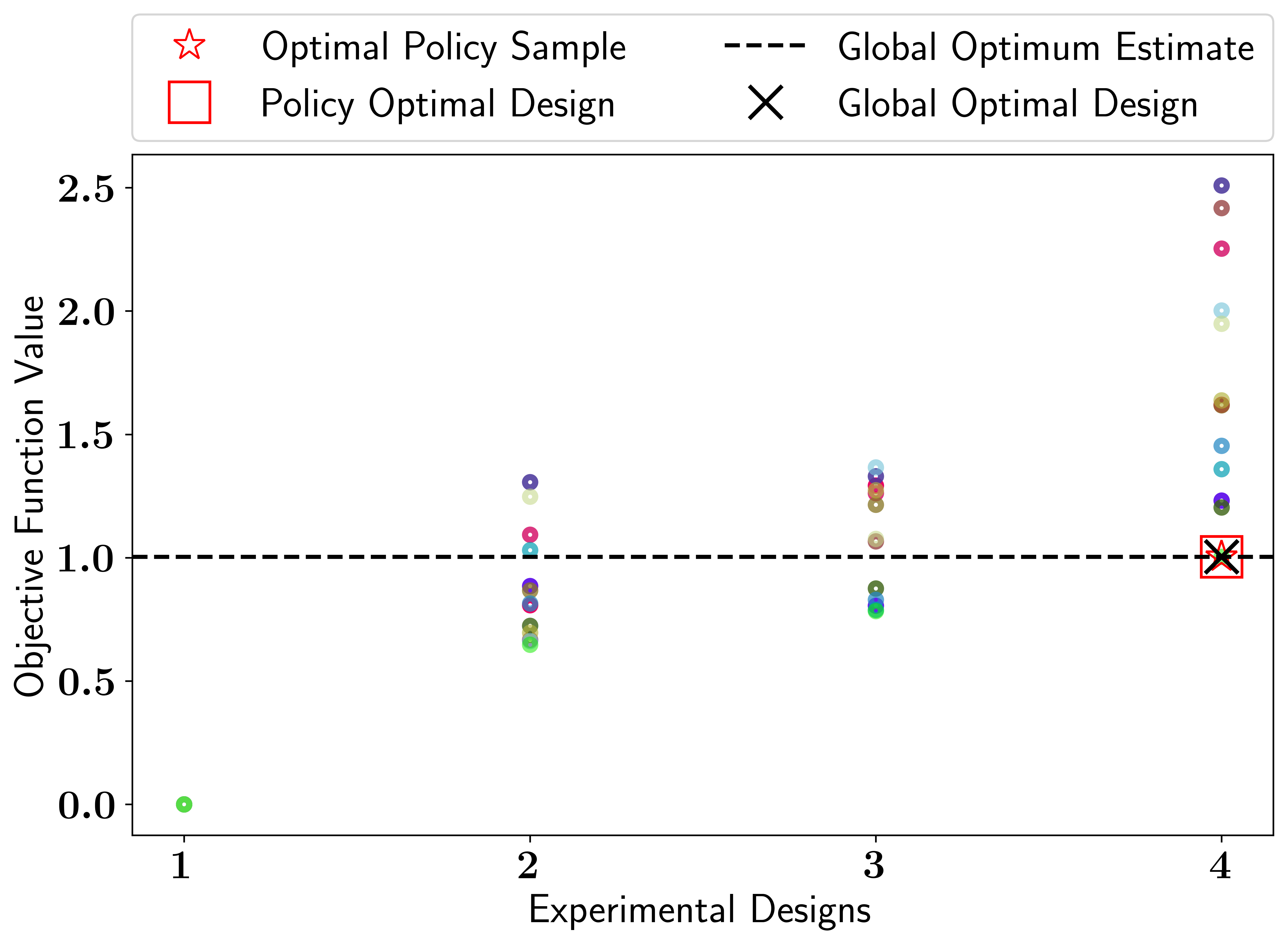
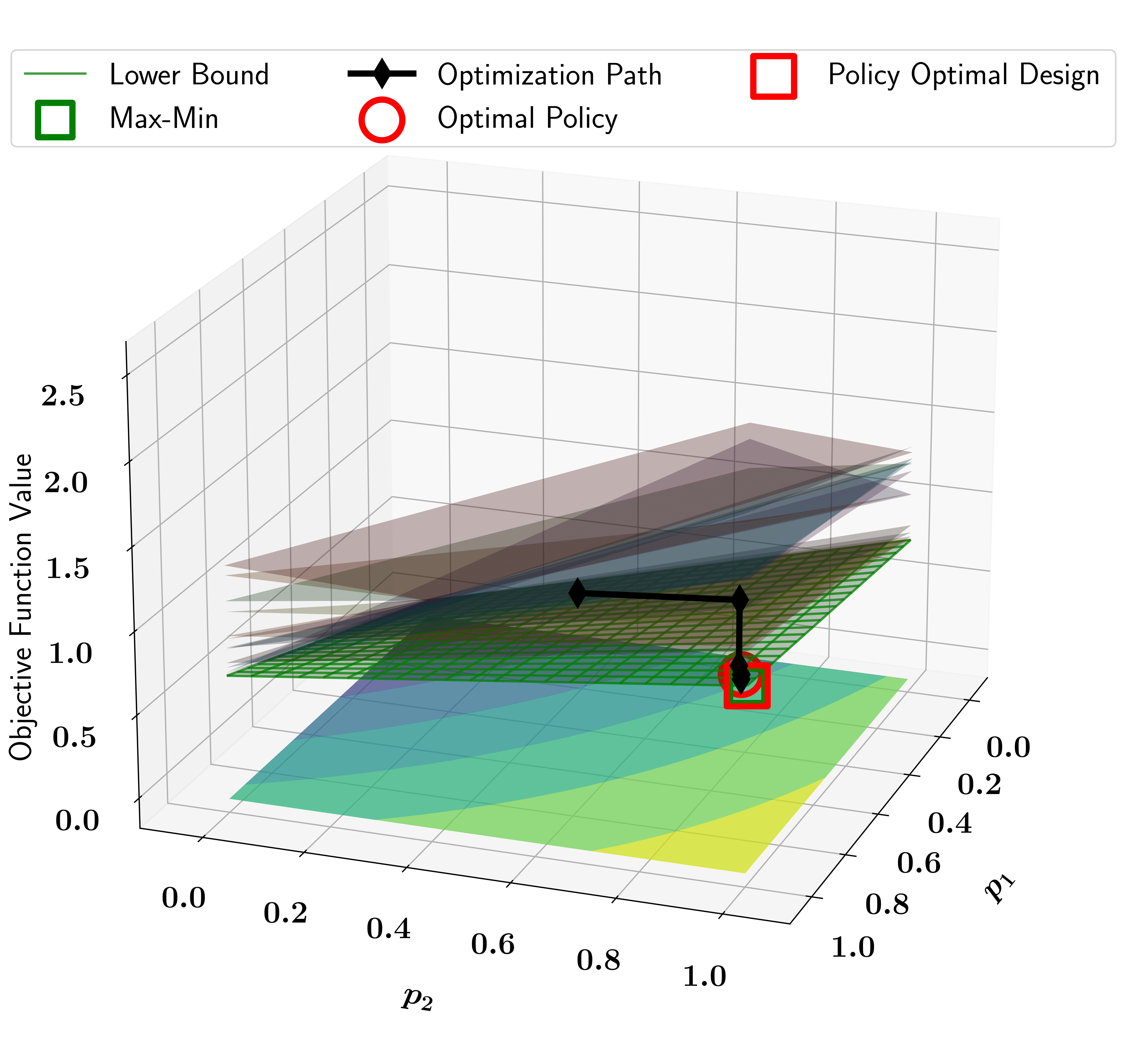
Figure 1: Results of the two sensor experiment. Left: Scatter plot of the utility $\mathcal{U}$ across designs, where different colors represent different realizations of $\bm{\theta}$. Right: Objective value surfaces where different color surface represents a different realization of $\bm{\theta}$.

As we have not imposed a budget, the optimal design is expected to be one with both sensors active $\bm{\xi}_{4}$. Indeed, in Figure 1 (left), we see that the optimal design discovered through Algorithm 1 is $\bm{\xi}^{\rm opt}=\bm{\xi}_{4}$. Additionally, we note that the optimal policy $\mathbf{p}_{\bm{\theta}}^{\rm opt}$ degenerates to the optimal design, as seen in Figure 1 (right). This is expected in a setting where the global optimal design is unique; see [9] for more details. Another interesting feature of this setting is that the utility $\mathcal{U}$ is not monotone in the noise parameters. Indeed, as both the scatter plot and the intersecting objective value surfaces in Figure 1 (right) indicate, different designs have different worst-case $\bm{\theta}$. This, critically, confirms the necessity for a robust optimization procedure. After all, if one could determine the worst-case $\bm{\theta}$ a priori, one could simply select those as a nominal value and perform a standard OED procedure.

4.2 64 Sensor, Budget 8, Experiment

Here, we consider an ROED setup with a realistic number of candidate sensors and a large number of uncertain parameters. Specifically, we consider the same simulation model as before, but with ${\rm N_{d}}=64$ candidate sensor locations forming a regular grid within the domain $\Omega$ and ${\rm N_{b}}=8$. Additionally, we consider an observation error covariance matrix $\mathbf{{\Gamma}}_{\rm n}$ whose entries are of the form:

(52a) $$(\Gamma_{\text{n}})_{ij}=\begin{cases}\sigma_{i}^{2}&\text{if }i=j\\ \sigma_{i}\sigma_{j}\rho_{ij}(\ell_{1},\ell_{2})&\text{if }i\neq j\end{cases}\,,$$

where

(52b) $$\rho_{ij}(\ell_{1},\ell_{2})=\exp\left(-\frac{1}{2\ell_{1}}|s_{i}^{(1)}-s_{j}^{(1)}|-\frac{1}{2\ell_{2}}|s_{i}^{(2)}-s_{j}^{(2)}|\right)\,,$$

with $$(s_{i}^{(1)},s_{i}^{(2)}) i \Theta=[0.05,0.15]^{64}\times[0.01,2.00]^{2}$$ denoting the coordinates of the th sensor. In this setting, .

In Figure 2, we report the optimization trajectory of Algorithm 1 and in Figure 3 we show the resulting optimal policy and optimal design. As demonstrated in Fig. 2, the algorithm took five total iterations of the outer / inner optimization process to converge, though the policy itself converged early during the third outer optimization stage. As such, the fourth and fifth outer optimization stages immediately terminated after a single outer optimization stage iteration. Note, in this experiment, the optimal policy did not degenerate; see Figure 3 (right). Likely, this is due to multiple designs producing similar utility. See the numerical results [7] for a similar observation for a different inverse problem.

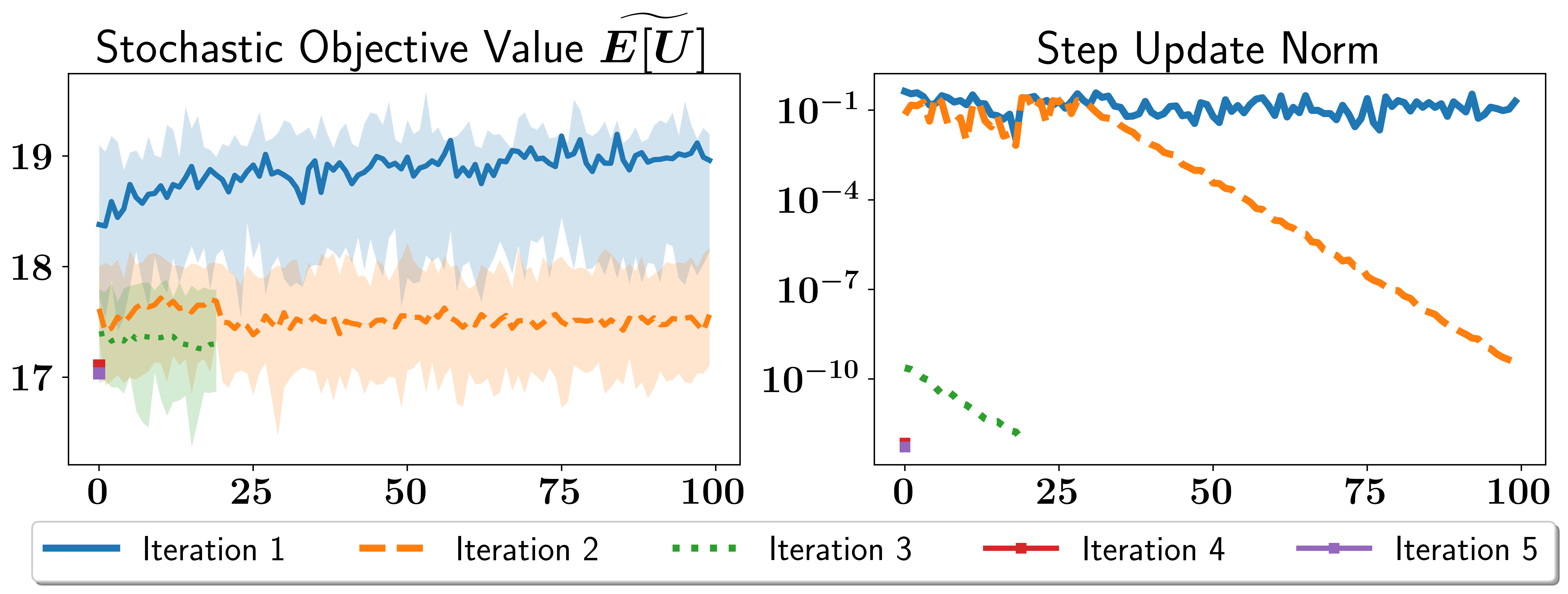
Figure 2: Optimization trajectory of the 64 sensor, budget 8, experiment. The iterations refer to those of the outer Polyak loop, and the x-axis refers to steps taken in the design optimization step of the inner Polyak loop. Left: Progress of an estimate to the expectation of the utility $\mathcal{U}$ over designs sampled from the policy at that iteration. The line represents the mean of the expectation whereas the top and bottom of the shaded region represent the maximum and minimum respectively. Right: Norm of the update in the policy $\mathbf{p}$ over the course of the algorithm.

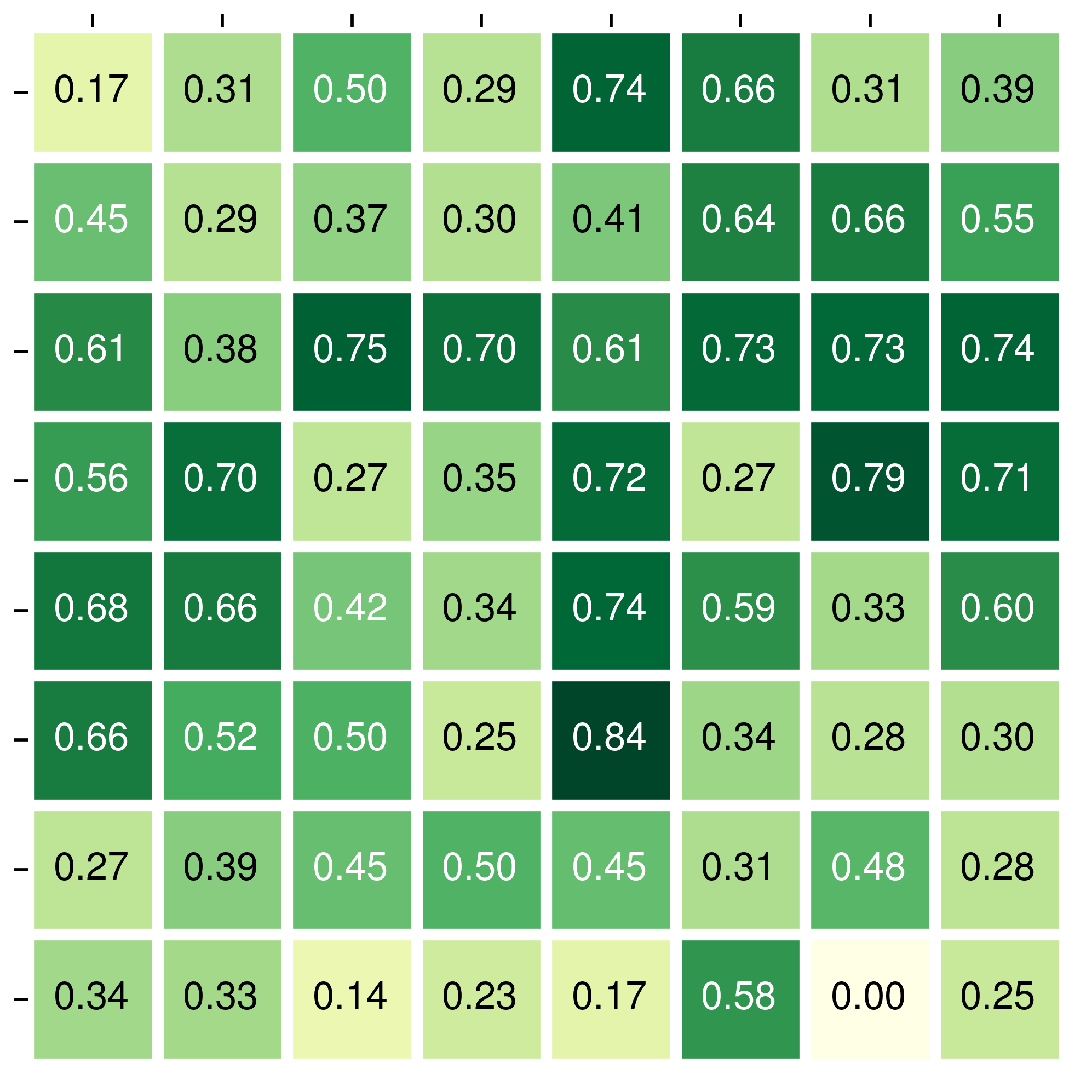
Figure 3: Results of the 64 sensor, budget 8, experiment. Left: Optimal design discovered by sampling from policy and selecting the design with the highest utility. Right: Optimal policy $\mathbf{p}_{\bm{\theta}}^{\rm opt}$ discovered by the stochastic optimization algorithm, visualized across the sensor grid.

To assess the effectiveness of the proposed strategy, we compare $\mathcal{U}(\bm{\xi}^{\rm opt},\bm{\theta}^{\rm opt})$ versus $\mathcal{U}(\bm{\xi},\bm{\theta}^{\rm opt})$ for ensemble of random designs. While it is not guaranteed that $\mathcal{U}(\bm{\xi}^{\rm opt},\bm{\theta}^{\rm opt})\geq\mathcal{U}(\bm{\xi},\bm{\theta}^{\rm opt})$ for all $\bm{\xi}\in\mathcal{S}({\rm N_{b}})$, the comparison is insightful. We do this comparison in Figure 4 (left). In the same figure, we also examine the optimality of the uncertain parameter by comparing against $\mathcal{U}(\bm{\xi}^{\rm opt},\bm{\theta})$ for random realizations of $\bm{\theta}$. For both comparisons, 64 random samples were used. We see that $\mathcal{U}(\bm{\xi}^{\rm opt},\bm{\theta}^{\rm opt})$ is significantly higher than that of $\mathcal{U}(\bm{\xi},\bm{\theta}^{\rm opt})$ for random designs. This indicates that the discovered design is nearly optimal. We see similar results for $\bm{\theta}^{\rm opt}$.

In Figure 4 (right), we repeat the above comparison using the utility $\overline{D_{\rm KL}^{(r)}}$. The results in the figure indicate that the optimality of $\bm{\xi}^{\rm opt}$ and $\bm{\theta}^{\rm opt}$ continue to hold. This provides numerical evidence regarding the effectiveness of the proposed strategy and the suitability of the proposed approximation framework. However, note that the scale of $\mathcal{U}$ and $\overline{D_{\rm KL}^{(r)}}$ are different.

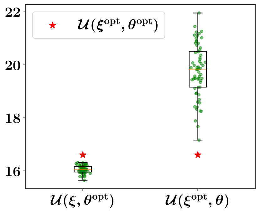
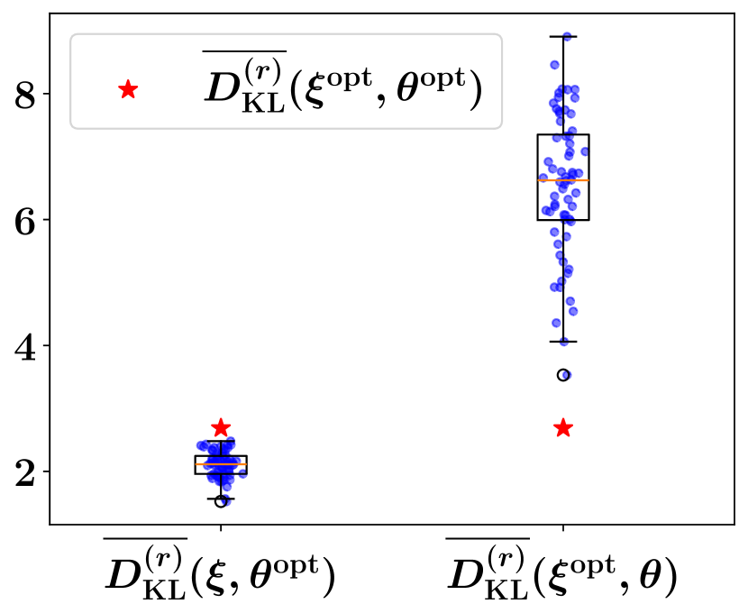
Figure 4: A visualization of the quality of $(\bm{\xi}^{\rm opt},\bm{\theta}^{\rm opt})$ for the 64 sensor, budget 8, ROED experiment. Here we compare the utility of $(\bm{\xi}^{\rm opt},\bm{\theta}^{\rm opt})$ against $(\bm{\xi}^{\rm opt},\bm{\theta})$ for random $\bm{\theta}$ and $(\bm{\xi},\bm{\theta}^{\rm opt})$ for random $\bm{\xi}$. These are evaluated using the utility $\mathcal{U}$ (left) and the low-rank EIG $\overline{D_{\rm KL}^{(r)}}$ (right).

5 Conclusion

In this article, we have outlined a scalable procedure for robust optimal design of large-scale Bayesian nonlinear inverse problems governed by PDEs. We have constructed a utility agnostic framework for the robust OED problem that is able to take advantage of the smaller space dictated by the budget. Then, for the case of the expected information gain used as the utility, we have developed a framework for its efficient approximation using variational tools in order to enable its efficient evaluation and differentiation.

There are various avenues for future work. In the first place, we may consider design criteria other than the expected information gain. Examples include generalizations of Bayesian A-optimality, goal-oriented design criteria, or decision theoretic ones such as the Bayes risk.

Secondly, the Laplace approximation and subsequent Gauss-Newton approximation to the Hessian were critical to the success of the proposed framework. However, while these are typically appropriate for many problems in practice, there is no guarantee that they will be appropriate for all problems. Particularly, consider posteriors which are multimodal or have heavy tails. In this case, an alternative approach may involve efficient surrogates of the simulation model. There has been significant work in this area regarding the use of neural networks as surrogates for governing equations given by PDEs, see [35]. An investigation into the use of such surrogates for the robust OED problem is an avenue for future work.

Finally, while the new budget-constrained ROED algorithm eliminates the major drawback of the penalty parameter tuning stage, there are still several avenues for improvement. For example, applying a probabilistic approach to the inner optimization stage could eliminate the need for developing bespoke gradients for the specific selection of utility and uncertain parameter. Likewise, leveraging different optimization approaches for outer optimization stage might also prove useful. For example, although relaxed OED approaches may not be suitable, the use of greedy or exchange type algorithms may prove to be a simple alternative; see, e.g., [29].

The submitted manuscript has been created by UChicago Argonne, LLC, Operator of Argonne National Laboratory (“Argonne”). Argonne, a U.S. Department of Energy Office of Science laboratory, is operated under Contract No. DE-AC02-06CH11357. The U.S. Government retains for itself, and others acting on its behalf, a paid-up nonexclusive, irrevocable worldwide license in said article to reproduce, prepare derivative works, distribute copies to the public, and perform publicly and display publicly, by or on behalf of the Government. The Department of Energy will provide public access to these results of federally sponsored research in accordance with the DOE Public Access Plan. http://energy.gov/downloads/doe-public-access-plan.

References

- [1] A. Alexanderian, Optimal experimental design for infinite-dimensional Bayesian inverse problems governed by PDEs: a review, Inverse Problems, 37 (2021), p. 043001.
- [2] A. Alexanderian, P. J. Gloor, and O. Ghattas, On Bayesian A- and D-optimal experimental designs in infinite dimensions, Bayesian Analysis, 11 (2016), pp. 671 – 695.
- [3] A. Alexanderian, R. Nicholson, and N. Petra, Optimal design of large-scale nonlinear Bayesian inverse problems under model uncertainty, Inverse Problems, (2024).
- [4] A. Alexanderian, N. Petra, G. Stadler, and I. Sunseri, Optimal design of large-scale Bayesian linear inverse problems under reducible model uncertainty: Good to know what you don’t know, SIAM/ASA Journal on Uncertainty Quantification, 9 (2021), pp. 163–184.
- [5] A. Alexanderian and A. K. Saibaba, Efficient D-optimal design of experiments for infinite-dimensional Bayesian linear inverse problems, SIAM Journal on Scientific Computing, 40 (2018), pp. A2956–A2985.
- [6] A. C. Atkinson and A. N. Donev, Optimum Experimental Designs, Oxford, 1992.
- [7] A. Attia, Probabilistic approach to black-box binary optimization with budget constraints: Application to sensor placement, arXiv preprint arXiv:2406.05830, (2024).
- [8] A. Attia and E. Constantinescu, Optimal experimental design for inverse problems in the presence of observation correlations, SIAM Journal on Scientific Computing, 44 (2022), pp. A2808–A2842.
- [9] A. Attia, S. Leyffer, and T. Munson, Robust A-optimal experimental design for Bayesian inverse problems, (2023), https://arxiv.org/abs/arXiv:2305.03855.
- [10] A. Attia, S. Leyffer, and T. S. Munson, Stochastic learning approach for binary optimization: Application to Bayesian optimal design of experiments, SIAM Journal on Scientific Computing, 44 (2022), pp. B395–B427.
- [11] W. Bangerth, A framework for the adaptive finite element solution of large-scale inverse problems, SIAM Journal on Scientific Computing, 30 (2008), pp. 2965–2989.
- [12] A. Bartuska, L. Espath, and R. Tempone, Small-noise approximation for Bayesian optimal experimental design with nuisance uncertainty, Comput. Methods Appl. Mech. Engrg., 399 (2022), p. 115320.
- [13] S. Biedermann and H. Dette, A note on maximin and Bayesian D-optimal designs in weighted polynomial regression, Mathematical Methods of Statistics, 12 (2003), p. 358–370.
- [14] T. Bui-Thanh, O. Ghattas, J. Martin, and G. Stadler, A computational framework for infinite-dimensional Bayesian inverse problems part i: The linearized case, with application to global seismic inversion, SIAM Journal on Scientific Computing, 35 (2013), pp. A2494–A2523.
- [15] K. Chaloner and I. Verdinelli, Bayesian experimental design: A review, Statistical Science, 10 (1995).
- [16] P. Chen, U. Villa, and O. Ghattas, Taylor approximation and variance reduction for pde-constrained optimal control under uncertainty, Journal of Computational Physics, 385 (2019), p. 163–186.
- [17] A. Chowdhary, S. E. Ahmed, and A. Attia, PyOED: An extensible suite for data assimilation and model-constrained optimal design of experiments, ACM Trans. Math. Softw., 50 (2024).
- [18] A. Chowdhary, S. Tong, G. Stadler, and A. Alexanderian, Sensitivity analysis of the information gain in infinite-dimensional Bayesian linear inverse problems, (2024).
- [19] D. R. Cox, Planning of Experiments, Wiley Classics Library, John Wiley & Sons, Nashville, TN, Apr. 1992.
- [20] Y. Daon and G. Stadler, Mitigating the influence of the boundary on PDE-based covariance operators, 2018.
- [21] J. E. Darges, A. Alexanderian, and P. A. Gremaud, Variance-based sensitivity of Bayesian inverse problems to the prior distribution, (2023). arXiv:2310.18488 [stat].
- [22] H. Dette, V. B. Melas, and A. Pepelyshev, Standardized maximin e-optimal designs for the michaelis-menten model, Statistica Sinica, 13 (2003), p. 1147–1163.
- [23] V. Fedorov, Optimal experimental design, WIREs Computational Statistics, 2 (2010), pp. 581–589.
- [24] N. Halko, P. G. Martinsson, and J. A. Tropp, Finding structure with randomness: Probabilistic algorithms for constructing approximate matrix decompositions, SIAM Review, 53 (2011), pp. 217–288.
- [25] J. Kaipio and V. Kolehmainen, Approximate marginalization over modeling errors and uncertainties in inverse problems, Bayesian Theory and Applications, (2013), pp. 644–672.
- [26] V. Kolehmainen, T. Tarvainen, S. R. Arridge, and J. P. Kaipio, Marginalization of uninteresting distributed parameters in inverse problems-application to diffuse optical tomography, International Journal for Uncertainty Quantification, 1 (2011).
- [27] K. Koval, A. Alexanderian, and G. Stadler, Optimal experimental design under irreducible uncertainty for linear inverse problems governed by PDEs, Inverse Problems, 36 (2020).
- [28] S. Kullback and R. A. Leibler, On information and sufficiency, The Annals of Mathematical Statistics, 22 (1951), pp. 79–86.
- [29] L. C. Lau and H. Zhou, A local search framework for experimental design, (2020).
- [30] P. D. Lax, Linear algebra and its applications, Pure and Applied Mathematics: A Wiley Series of Texts, Monographs and Tracts, Wiley-Blackwell, Chichester, England, 2 ed., Aug. 2007.
- [31] E. Levitin and B. Polyak, Constrained minimization methods, USSR Computational Mathematics and Mathematical Physics, 6 (1966), pp. 1–50.
- [32] D. C. Liu and J. Nocedal, On the limited memory BFGS method for large scale optimization, Mathematical Programming, 45 (1989), p. 503–528.
- [33] A. Logg, K.-A. Mardal, and G. Wells, Automated Solution of Differential Equations by the Finite Element Method: The FEniCS Book, vol. 84 of Lecture Notes in Computational Science and Engineering, Springer Berlin Heidelberg, Berlin, Heidelberg, 2012.
- [34] M. Mozumder, T. Tarvainen, S. Arridge, J. P. Kaipio, C. D’Andrea, and V. Kolehmainen, Approximate marginalization of absorption and scattering in fluorescence diffuse optical tomography, Inverse Problems & Imaging, 10 (2016), p. 227.
- [35] T. O’Leary-Roseberry, U. Villa, P. Chen, and O. Ghattas, Derivative-informed projected neural networks for high-dimensional parametric maps governed by PDEs, Computer Methods in Applied Mechanics and Engineering, 388 (2022), p. 114199.
- [36] R.-E. Plessix, A review of the adjoint-state method for computing the gradient of a functional with geophysical applications, Geophysical Journal International, 167 (2006), pp. 495–503.
- [37] L. Pronzato and E. Walter, Robust experiment design via maximin optimization, Mathematical Biosciences, 89 (1988), pp. 161–176.
- [38] T. Rainforth, A. Foster, D. R. Ivanova, and F. B. Smith, Modern Bayesian Experimental Design, Statistical Science, 39 (2024), pp. 100 – 114.
- [39] C. R. Rojas, J. S. Welsh, G. C. Goodwin, and A. Feuer, Robust optimal experiment design for system identification, Automatica, 43 (2007), pp. 993–1008.
- [40] A. M. Stuart, Inverse problems: A Bayesian perspective, Acta Numerica, 19 (2010), p. 451–559.
- [41] I. Sunseri, A. Alexanderian, J. Hart, and B. v. B. Waanders, Hyper-differential sensitivity analysis for nonlinear Bayesian inverse problems, International Journal for Uncertainty Quantification, 14 (2024), p. 1–20.
- [42] D. Telen, F. Logist, E. Van Derlinden, and J. F. Van Impe, Robust optimal experiment design: A multi-objective approach, IFAC Proceedings Volumes, 45 (2012), pp. 689–694. 7th Vienna International Conference on Mathematical Modelling.
- [43] D. Telen, D. Vercammen, F. Logist, and J. Van Impe, Robustifying optimal experiment design for nonlinear, dynamic (bio)chemical systems, Computers & Chemical Engineering, 71 (2014), pp. 415–425.
- [44] D. Uciński, Optimal measurement methods for distributed parameter system identification, Systems and Control Series, CRC Press, Boca Raton, FL, 2005.
- [45] U. Villa, N. Petra, and O. Ghattas, HIPPYlib: An Extensible Software Framework for Large-Scale Inverse Problems Governed by PDEs: Part I: Deterministic Inversion and Linearized Bayesian Inference, ACM Trans. Math. Softw., 47 (2021).
- [46] A. Wald, Statistical decision functions which minimize the maximum risk, Annals of Mathematics, 46 (1945), p. 265–280.
- [47] K. Wu, P. Chen, and O. Ghattas, A fast and scalable computational framework for large-scale high-dimensional bayesian optimal experimental design, SIAM/ASA Journal on Uncertainty Quantification, 11 (2023), pp. 235–261.