EW corrections and Heavy Boson Radiation at a high-energy muon collider

Abstract

In this work we investigate several phenomenological and technical aspects related to electroweak (EW) corrections at a high-energy muon collider, focusing on direct production processes (no VBF configurations). We study in detail the accuracy of the Sudakov approximation, in particular the Denner-Pozzorini algorithm, comparing it with exact calculations at NLO EW accuracy. We also assess the relevance of resumming EW Sudakov logarithms (EWSL) at 3 and 10 TeV collisions. Furthermore, we scrutinise the impact of additional Heavy Boson Radiation (HBR), namely the weak emission of $W,Z$, and Higgs bosons in inclusive and semi-inclusive configurations. All results are obtained via the fully automated and publicly available code MadGraph5_aMC@NLO.

1 Introduction

In recent years a novel interest for a muon collider has arisen, motivated by its great potential for the investigation of the fundamental interactions of Nature MuonCollider:2022xlm ; Aime:2022flm ; Black:2022cth ; Maltoni:2022bqs ; Belloni:2022due ; Accettura:2023ked . A key aspect of a muon collider is the possibility of accelerating elementary particles at energies of several TeV’s Delahaye:2019omf ; Bartosik:2020xwr ; Schulte:2021hgo ; Long:2020wfp ; MuonCollider:2022nsa ; MuonCollider:2022ded ; MuonCollider:2022glg , leading to the possibility to probe fundamental interactions at unprecedented energies. It offers the potential to significantly advance our understanding of fundamental particle physics, enabling in-depth studies of the Standard Model (SM) Higgs boson Han:2020pif ; Buttazzo:2020uzc ; Han:2021lnp ; Reuter:2022zuv ; Celada:2023oji ; Forslund:2022xjq ; Chen:2022yiu ; Ruhdorfer:2023uea ; Han:2023njx ; Dermisek:2023rvv ; Liu:2023yrb ; Li:2024joa , searches for beyond-the-SM (BSM) heavy Higgs bosons Han:2022edd ; Bandyopadhyay:2020otm ; Han:2021udl ; Bandyopadhyay:2024plc ; Ouazghour:2023plc ; Jueid:2023qcf , investigations of dark matter Han:2020uak ; Capdevilla:2021fmj ; Han:2022ubw ; Cesarotti:2024rbh ; Asadi:2023csb ; Belfkir:2023vpo ; Jueid:2023zxx , constraints on lepton-universality violation Huang:2021nkl ; Huang:2021biu ; He:2024dwh , exploration of the muon $g-2$ anomaly Buttazzo:2020ibd ; Capdevilla:2020qel ; Yin:2020afe ; Capdevilla:2021rwo , and tests of a wide range of new physics scenarios Gu:2020ldn ; Costantini:2020stv ; Bandyopadhyay:2021pld ; Qian:2021ihf ; Bao:2022onq ; Ghosh:2023xbj ; Dermisek:2023tgq ; Altmannshofer:2023uci ; Liu:2023jta ; Sun:2023cuf ; Kwok:2023dck ; Cesarotti:2023sje ; Ema:2023buz ; Li:2023tbx .

A muon collider is therefore both a discovery and precision machine. In particular, precision physics relies on both a clean experimental environment (no QCD in the initial state) and precise and reliable theoretical predictions. Thus, as has been the case for LEP, the calculation of electroweak (EW) corrections will be paramount for theoretical predictions in muon collisions. In fact, unlike other possible future electron-positron colliders, e.g. the Future Circular Collider (FCC-ee) FCC:2018evy ; Bernardi:2022hny and the Circular Electron-Positron Collider (CEPC) CEPCStudyGroup:2018rmc ; CEPCStudyGroup:2018ghi ; An:2018dwb ; CEPCAcceleratorStudyGroup:2019myu ; CEPCPhysicsStudyGroup:2022uwl ; CEPCStudyGroup:2023quu , at a high-energy muon collider the scope and relevance of EW corrections will be much broader, especially for a 10 TeV (or higher) collision machine. EW corrections at high energies can be very large, even of ${\cal O}(1)$ w.r.t. the leading-order (LO) prediction, and therefore are expected to be unavoidable in any phenomenological study, not only those regarding precision. The origin of such enhancements is the so-called EW Sudakov logarithms (EWSL), which involve logarithms of ratios of the form $Q/M_{W}$, where $Q$ is any of the scale of the process, like the energy of the collider $\sqrt{S}$, and $M_{W}$ is the $W$ boson mass.

On the one hand, such logarithms emerge from the real emission of heavy bosons $V=W,Z$ (and $H$). It has been shown that such mechanism can be exploited in order to leverage the sensitivity on BSM effects in the hard process Buttazzo:2020uzc ; Chen:2022msz and in general it has become a widespread notion that these effects will be ubiquitous in the muon collider physics AlAli:2021let . Above all, the idea of the muon collider as a vector-boson collider has emerged, where Vector-Boson-Fusion (VBF) processes can be modelled directly via $VV$ initiated processes and the convolution of universal and process-independent parametrisations of the $V$ emission from initial-state muons Costantini:2020stv ; Ruiz:2021tdt . Different groups have already calculated and provided EW PDFs of $V$ bosons (and the other particles of the SM spectrum) in the muon Han:2020uid ; Han:2021kes ; Garosi:2023bvq , resumming such effects.

On the other hand, EWSL originate from “genuine” EW corrections, i.e., loop diagrams Sudakov:1954sw . The calculation of such logarithms has also received a novel interest in the past years, independently from the muon-collider physics. An algorithmic procedure for the evaluation of EWSL at one- Denner:2000jv ; Denner:2001gw and two-loop Denner:2003wi ; Denner:2004iz ; Denner:2006jr ; Denner:2008yn accuracy, the so-called Denner and Pozzorini (DP) algorithm, has been available for a long time. Such algorithm has been automated for the first time Bothmann:2020sxm in the Sherpa framework Sherpa:2019gpd and extended to the case of multijet merging at the next-to-leading order (NLO). Afterward, the DP algorithm has been revisited and improved in particular features Pagani:2021vyk and automated within the MadGraph5_aMC@NLO framework Alwall:2014hca ; Frederix:2018nkq and matched to NLO+PS simulations in QCD Pagani:2023wgc . Very recently Lindert:2023fcu , it has been automated also in the OpenLoops framework Cascioli:2011va ; Buccioni:2019sur , and adapted for a dynamical treatment of resonances.

The resummation of EWSL has also been studied and in Refs. Chiu:2007yn ; Chiu:2008vv ; Manohar:2018kfx a general method to resum such logarithms for an arbitrary process was developed, based on the framework of soft-collinear effective theory (SCET) Bauer:2000ew ; Bauer:2000yr ; Bauer:2001ct ; Bauer:2001yt . Very recently, in Ref. Denner:2024yut , NLL resummation has been implemented in realistic Monte Carlo simulations and studied both in the context of future leptonic (CLIC at 3 TeV Aicheler:2012bya ; Linssen:2012hp ; Lebrun:2012hj ; CLIC:2016zwp ; CLICdp:2018cto ; Brunner:2022usy ) and hadronic (FCC-hh at 100 TeV FCC:2018byv ; FCC:2018vvp ; Benedikt:2022kan ) colliders.

One of the reasons for the novel interest in the computation of EWSL is the fact that they can in principle approximate very well the exact NLO EW corrections, but their evaluation does not involve the explicit computation of loop diagrams; only tree-level amplitudes and logarithms are involved. Thus, the evaluation of EWSL is much faster and easier. Besides the SM scenario, their evaluation has been performed also for BSM scenarios, such as Dark-Matter studies Ciafaloni:2010ti , and it is clearly relevant in the context of a high-energy muon collider, as shown e.g. in the already mentioned Refs. Buttazzo:2020uzc ; Chen:2022msz .

Both for the SM and BSM case, one should keep in mind that the EWSL are an approximation. Knowing how efficient is this approximation is of primary relevance for physics at a high-energy muon collider. However, nowadays also the automation of the exact NLO EW corrections is available for SM processes, both in hadronic and leptonic collisions Alwall:2014hca ; Kallweit:2014xda ; Frixione:2015zaa ; Chiesa:2015mya ; Biedermann:2017yoi ; Chiesa:2017gqx ; Frederix:2018nkq ; Pagani:2021iwa ; Bertone:2022ktl ; Bredt:2022dmm . Thus, it is possible to compare directly EWSL and exact NLO EW corrections in order to assess their level of accuracy for SM processes.

In this work, we precisely investigate this issue for the case of a muon collider at 3 and 10 TeV. We focus on direct production processes (also denoted in the literature as muon-muon annihilation), $\mu^{+}\mu^{-}\to F$, where the invariant mass of the final state is close to the energy of the collider and therefore VBF configurations are suppressed. In these configurations the only relevant PDFs are the ones of the (anti)muon in the (anti)muon, which accounts for effects from QED initial-state radiation (ISR). Moreover, our focus is not on precision physics but on large effects, as those expected from EWSL at high energies. We exploit the SM as a “test case”, but our conclusions are instructive also for a general BSM scenario. All our calculations are performed via the MadGraph5_aMC@NLO framework Alwall:2014hca ; Frederix:2018nkq ; Pagani:2021vyk ; Bertone:2022ktl , in a completely automated approach.

First of all, we investigate in detail how accurate is the Sudakov approximation and in particular its evaluation via the DP algorithm, comparing it with exact NLO EW results. In particular, the DP algorithm has been rigorously derived for the approximation of one-loop amplitudes in the strict limit $M_{W}^{2}/s\to 0$, but its application for physical observables is less straightforward and has been revisited in Ref. Pagani:2021vyk . On the one hand, it has shown that the usage of the so-called ${\rm SDK_{weak}}$ scheme, a purely weak version of the original one, can be superior to the more commonly used ${\rm SDK_{0}}$ scheme when charged particles in the final state are recombined with photons. On the other hand, it has shown that logarithms such as $\log^{2}(s/|t|)$ or $\log^{2}(s/|u|)$, and in general logarithms involving ratios of Lorentz invariants of the process, can be numerically very large and the assumptions as $s\simeq|t|\simeq|u|$ are not efficient. We address both these aspects when comparing EWSL and exact NLO EW corrections. Moreover, we show a specific case for a process ($\mu^{+}\mu^{-}\to ZHH$ production) where in some regions of the phase space the LO predictions are numerically dominated by diagrams that are mass-suppressed in the $M_{W}^{2}/s$ expansion, such that the DP algorithm lies outside its range of applicability and therefore returns wrong results. Such an example is very counterintuitive, and the Sudakov approximation is very efficient in the region where one would not naively expect it, and vice versa.

Then we approximate the resummation of EWSL via a simple exponentiation and, after additively matching them to the exact NLO EW, we compare this prediction with the exact NLO EW itself. We investigate when resummation is expected to be relevant only for precision studies and when instead is unavoidable in order to obtain sensible predictions, especially positive defined.

Finally, we scrutinise the contribution of Heavy-Boson-Radiation (HBR), in other words the emission of weak bosons $W,Z$, and $H$. We consider different scenarios, where HBR is recombined or not with particles in the final state $F$ in $\mu^{+}\mu^{-}\to F$ production. We also consider as physical objects in the final state $F$ the so-called “EW jets”, obtained by the clustering of $W$ and $Z$ bosons. We compare the impact of HBR, which is calculated exactly and taking into account phase-space cuts, with the one of NLO EW corrections, also calculated exactly, and discuss their relative size and possible cancellations. We show how HBR leads in general to much smaller contributions than their virtual counterparts, only marginally compensating for the large effects due to the latter.

The paper is structured as described in the following. In Sec. 2 we briefly summarise the automation of both NLO EW corrections and EWSL in MadGraph5_aMC@NLO, focusing on the aspects relevant to the study presented in this work. In Sec. 3 we describe in detail our calculation setup and the definitions of the different approximations used. Also, we better formalise the aspects that we want to investigate in this work and that we have mentioned in the previous paragraphs. All the numerical results and the discussion of the information obtained are reported in Sec. 4. We give our conclusions in Sec. 5.

2 NLO EW corrections and EWSL in MadGraph5_aMC@NLO

2.1 The automation of NLO EW corrections

Given a physical observable, typically a cross section, the so-called NLO QCD and NLO EW corrections correspond to the exact ${\cal O}(\alpha_{s})$ and ${\cal O}(\alpha)$ corrections, respectively, to its LO prediction.  Such corrections involve the calculation of one-loop amplitudes, their renormalisation, the regularisation of IR divergencies, and the combination of virtual as well as real-emission contributions in order to cancel them.

The automatic computation of NLO QCD and EW corrections, and the matching of the former to parton-shower, is a well-known feature of the metacode MadGraph5_aMC@NLO, achieved both for hadronic Frederix:2018nkq ; Pagani:2021iwa and leptonic Bertone:2022ktl collisions. Before delving into aspects specific to muon colliders, we remind the reader of some general features about the building blocks of the code. The computation of NLO corrections requires the local subtraction of IR singularities and the numerical evaluation of one-loop amplitudes. The first task is achieved using the FKS subtraction scheme Frixione:1995ms ; Frixione:1997np as implemented in MadFKS Frederix:2009yq ; Frederix:2016rdc . The second task builds upon a number of different numerical techniques (integrand reduction Ossola:2006us , tensor-integral reduction Passarino:1978jh ; Davydychev:1991va ; Denner:2005nn , Laurent-series expansion Mastrolia:2012bu , and an in-house implementation of the OpenLoops method Cascioli:2011va ), implemented in publicly-available software libraries Ossola:2007ax ; ShaoIREGI ; Peraro:2014cba ; Hirschi:2016mdz ; Denner:2014gla ; Denner:2016kdg , all steered by the MadLoop module Hirschi:2011pa . Matching to parton shower (not relevant for the work in this paper) is performed using the MC@NLO method Frixione:2002ik .

The capabilities of MadGraph5_aMC@NLO in the computation of EW corrections at hadron colliders have been documented in a number of papers  Frixione:2014qaa ; Frixione:2015zaa ; Pagani:2016caq ; Frederix:2016ost ; Czakon:2017wor ; Czakon:2017lgo ; Frederix:2017wme ; Frederix:2018nkq ; Broggio:2019ewu ; Frederix:2019ubd ; Pagani:2020rsg ; Pagani:2020mov ; Pagani:2021iwa ; Pagani:2021vyk ; Frederix:2021agh ; Frederix:2021zsh . For what concerns EW corrections at lepton-lepton colliders, either electron-positron or muon-antimuon ones, far fewer results are available, and are limited only to the case of electron-positron colliders. We will first review these results, and then comment on how to extend them at muon colliders. For electron-positron colliders, in MadGraph5_aMC@NLO effects due to initial-state radiation (ISR) are included in a collinear-inspired picture, i.e., using quantities analogous to the partonic density functions (PDFs) at hadron colliders. At variance with their hadronic counterpart, leptonic PDFs are perturbative and can thus be computed via first principles. This requires the knowledge of their initial conditions, on which one applies the DGLAP evolution. The computation of NLO initial conditions Frixione:2019lga has led to the availability of leptonic PDFs whose accuracy is Next-to-Leading-Logarithmic (NLL) Bertone:2019hks ; Frixione:2012wtz ; Bertone:2022ktl . In Ref. Bertone:2022ktl in particular, the dependence on physical cross sections on renormalisation and factorisation schemes has been thoroughly scrutinised for a selection of lepton-initiated processes. This required the computation of the corresponding cross sections at NLO accuracy, which has been performed using a new version (now public) of MadGraph5_aMC@NLO. The most relevant difference w.r.t. the hadronic case, which required adaptation of the phase-space integration, stems from the asymptotic behaviour of lepton PDFs at large values of the Bjorken $x$ variable. While hadronic PDFs typically vanish in the limit $x\to 1$, leptonic PDFs feature an integrable singularity in the same limit:

$$\lim_{x\to 1}\Gamma_{e^{-}/e^{-}}(x,Q^{2})=C(1-x)^{\beta-1}\,,$$ (2.1)

where $\beta\sim 0.05$ (more details will be given in Appendix A). Owing to the (distribution) identity

$$(1-x)^{\beta-1}=\frac{1}{\beta}\delta(1-x)+\left.\frac{1}{1-x}\right|_{+}+\mathcal{O}(\beta)\,,$$ (2.2)

one can easily see that the bulk of the cross section comes from regions where $x\to 1$. The peculiar dependence of the leptonic PDFs required some changes in MadGraph5_aMC@NLO, in order to have an efficient numerical integration: the first, trivial, is to flatten out the integrable divergence via a suitable change of integration variables Frixione:2021zdp . The second one specific to the computation of NLO EW corrections, is to devise a phase-space mapping where the event and its soft/collinear counterterms are evaluated at the same values of the Bjorken $x$. Such a new mapping is documented in the appendix of Ref. Bertone:2022ktl . Finally, the existence of NLL densities in different factorisation schemes requires the inclusion in the short-distance cross section of additional terms (finite contributions to the initial-state counterterms). The same applies to the case when LL-accurate PDFs are employed, in order to attain formal NLO accuracy.

Turning specifically to muon colliders, in principle most of what has been achieved for electron-positron ones can be trivially extended. Two caveats here are in order, both related to the higher energy of which muon colliders are capable: first, the Bjorken-$x$ range is extended towards much smaller values, a fact that leads to enhancements of partonic channels that would be otherwise suppressed. Indeed, at small $x$ ($x\lesssim 10^{-2}$ for a 10 TeV muon collider) on top of densities related to purely QED-interacting partons (photons and singlet contribution, related e.g. to the positron inside the electron), also those of QCD-interacting ones (quarks and gluons) can lead to non-negligible contributions Han:2020uid ; Han:2021kes ; Aime:2022flm ; BuarqueFranzosi:2021wrv . Moreover, also the contributions from $W,Z$, and Higgs bosons as well as neutrinos PDFs have been studied Han:2020uid ; Han:2021kes ; Garosi:2023bvq and found to be relevant, especially for very high energies. Second, effects due to EW corrections are sizeable (typically much larger than 10% of the LO and reaching even more than 100% in absolute value), and their inclusion is mandatory even for ${\cal O}(1)$ estimates of the cross sections.

In view of these facts, and considering that this work represents a starting point in the study, within the MadGraph5_aMC@NLO framework, of EW effects at muon colliders, we will focus on the kinematics region where the non-singlet muon density dominates, i.e. large Bjorken-$x$. This will be achieved by an invariant-mass cut on the final-state products. Besides, also considering the current unavailability of NLL PDFs for muon colliders, we will not discuss effects due to the renormalisation- or factorisation-scheme employed in the PDFs. Given their size at electron-positron colliders, see Ref. Bertone:2022ktl , their effects are expected to be negligible w.r.t. the size of the EW corrections that we calculate and discuss in this work.

2.2 EWSL: the implementation of the DP algorithm

We recall in this section the main features of the DP algorithm Denner:2000jv ; Denner:2001gw , and its revisitation presented in Ref. Pagani:2021vyk , as implemented in MadGraph5_aMC@NLO. Many more details can be found in Ref. Pagani:2021vyk and, part of them, also in the Appendix A of Ref. Pagani:2023wgc .

2.2.1 Amplitude level

When the high-energy limit $s\gg M_{W}^{2}$ is considered, the DP algorithm allows for the calculation of the leading contributions of the one-loop EW corrections of a generic SM scattering amplitude. These contributions are denoted as the “leading approximation” (LA), which consists of double-logarithmic (DL) and single-logarithmic (SL) corrections, both from IR and UV origin, of the form

$$L(|r_{kl}|,M^{2})\equiv\frac{\alpha}{4\pi}\log^{2}{\frac{|r_{kl}|}{M^{2}}}\qquad{\rm and}\qquad l(|r_{kl}|,M^{2})\equiv\frac{\alpha}{4\pi}\log{\frac{|r_{kl}|}{M^{2}}}\,.$$ (2.3)

Such logarithms are precisely what we denote as the EWSL. In Eq. (2.3), $r_{kl}$ is a generic kinematic invariant $r_{kl}\equiv(p_{k}+p_{l})^{2}$ involving the momenta of a pair of external particles (all momenta defined as incoming) and $M$ is any of the masses of the SM heavy particles ($M_{W},M_{H},$ $m_{t}$ and $M_{Z}$) or the IR-regularisation scale $Q$, for the case of purely QED contributions involving photons.

Via the DP algorithm it is possible to calculate in LA one-loop EW corrections of a generic SM scattering amplitude ${\cal{M}}$, which are typically denoted as $\delta{\cal{M}}$, to the Born approximation, which is instead typically denoted as ${\cal{M}}_{0}$. For any individual helicity configuration of the amplitude ${\cal{M}}$, the DP algorithm allows to write $\delta{\cal{M}}$ as a function of the logarithms in Eq. (2.3), the couplings of each external field to the gauge bosons (and another possible field) or associated quantities such as electroweak Casimir operators, and tree-level amplitudes as ${\cal{M}}_{0}$ or similar ones with one or two of the external fields replaced by, e.g., $SU(2)$ partners w.r.t. the case of ${\cal{M}}_{0}$. This is precisely at the origin of the resurgence of the interest in EWSL and the DP algorithm in the past few years: EWSL can be computed in a much faster and more stable way than the exact NLO EW corrections and this approach can be (supposedly) extended to the BSM case, capturing the leading corrections at high energies.

However, there are a few crucial assumptions that underly the derivation of the DP algorithm and we list them in the following:

• External legs must be on-shell.

• All the invariants are much larger in absolute value than the typical EW scale, namely,

  $$|r_{kl}|\equiv|(p_{k}+p_{l})^{2}|\simeq|2p_{k}p_{l}|\gg M_{W}^{2}\simeq M_{H}^{2},m_{t}^{2},M_{W}^{2},M_{Z}^{2}.$$ (2.4)

  Therefore the case of resonant decays is excluded.

• For the helicity configuration considered, in the high-energy limit, the tree-level amplitude ${\cal{M}}_{0}$ must not be mass-suppressed by powers of the form $(M_{W}/\sqrt{s})^{k}$ with $k>0$. In other words, by dimensional analysis, a $2\rightarrow n$ process requires that $[{\cal{M}}]=(\,\textrm{GeV})^{2-n}$ and therefore

  $${\cal{M}}\propto s^{\frac{2-n}{2}}\,,$$ (2.5)

  with no extra $(M_{W}/\sqrt{s})^{k}$ powers.

An additional assumption is also present in the strict LA as derived in Refs. Denner:2000jv ; Denner:2001gw , namely, if a specific $r_{k^{\prime}l^{\prime}}$ in a given process is considered, then the condition

$$|r_{kl}|/|r_{k^{\prime}l^{\prime}}|\simeq 1\,,$$ (2.6)

is always assumed, such that logarithms of the form $\log(r_{kl}/r_{k^{\prime}l^{\prime}})$ are always discarded unless they multiply other logarithms of the kind in (2.3).

The last point has been addressed in detail in Ref. Pagani:2021vyk , where it has been shown  that not only the logarithms of the form $L(s,M_{W}^{2})$ and $l(s,M_{W}^{2})$, but also those of the form $L(r_{kl},r_{k^{\prime}l^{\prime}})$ and $l(r_{kl},r_{k^{\prime}l^{\prime}})$ can be relevant, especially when

$$|r_{kl}|\gg|r_{k^{\prime}l^{\prime}}|\gg M_{W}^{2}\,.$$ (2.7)

The former two kinds of logarithms yield the formal LA as presented in Refs. Denner:2000jv ; Denner:2001gw , while the latter ones have been reintroduced in the DP algorithm in the revisitation in Ref. Pagani:2021vyk and they have been denoted as the $\Delta^{s\rightarrow r_{kl}}$ contribution therein. Afterward, they have been employed in the literature also in Ref. Bothmann:2021led and in Ref. Lindert:2023fcu , where they have been denoted as the sub-subleading soft collinear corrections (S-SSC) beyond the strict LA. Unlike the strict LA, the $\Delta^{s\rightarrow r_{kl}}$ has not been derived via formal arguments and in principle some logarithms of the same form may be missed; they have to be checked case by case, but so far all the comparisons with the exact calculation of virtual corrections, presented e.g. in Refs. Pagani:2021vyk ; Lindert:2023fcu , have shown a (sometimes dramatic) improvement in the agreement of exact calculation and the EWSL approximation when they are included. Therefore, for simplicity, we will refer in the following to LA regardless of the inclusion or not of the $\Delta^{s\rightarrow r_{kl}}$ terms.

Before considering the case of squared matrix elements and cross sections it is important to note that, as we have already said, the logarithms in Eq. (2.3) can be of the form $\log(|r_{kl}|/Q^{2})$ or, using a fictitious photon mass $\lambda$ as an infrared regulator as done in Refs. Denner:2000jv ; Denner:2001gw , of the form $\log(M_{W}^{2}/\lambda^{2})$. Needless to say, such quantity and consequently $\delta{\cal{M}}$ is IR-divergent and therefore non-physical, similar to the virtual corrections without any approximation. A prescription or further additional steps are therefore necessary and discussed in the next subsection.

2.2.2 Cross-section level

What has been discussed in the previous section is here extended and projected to the case of squared matrix elements and especially to the cross-section level. We will focus here on the case of the muon collider and will consider only processes that are of purely EW origin.

The squared amplitude $|{\cal{M}}|^{2}$ of a given process can be directly linked to the fully differential cross section $\Sigma$. For brevity, we will consider only $\Sigma$ in the following discussion, again more details can be found in Refs. Pagani:2021vyk ; Pagani:2023wgc . If we denote the LO prediction of $\Sigma$ as $\Sigma_{{\rm LO}}$ and its purely virtual NLO EW corrections as $\Sigma^{\rm virt}_{\rm NLO_{EW}}$, in the LA we obtain

$$(\Sigma^{\rm virt}_{\rm NLO_{EW}})\Big{|}_{\rm LA}=\Sigma_{{\rm LO}}\delta^{\rm EW}_{\rm LA}\,,$$ (2.8)

with

$$\delta^{\rm EW}_{\rm LA}\equiv\frac{2\real({\cal{M}}_{0}\delta{\cal{M}}^{*})}{|{\cal{M}}_{0}|^{2}}\,,$$ (2.9)

where ${\cal{M}}_{0}$ is the amplitude that once squared leads precisely to $\Sigma_{{\rm LO}}$.

Since $\delta^{\rm EW}_{\rm LA}$ is an approximation of the relative virtual EW corrections to the LO, it involves photons and therefore it is IR-divergent and non-physical as the quantity $\delta{\cal{M}}$. Thus, it cannot be used, as it is, for a comparison with the exact NLO EW corrections, which instead involve also real emission contributions and are IR safe. Such comparison is however one of the main aspects that we want to investigate in this paper in the context of muon-collider physics. For this purpose, it is first of all useful to distinguish three different schemes for the calculation of the EWSL, specifying their relation with NLO EW corrections for physical cross sections:

• SDK: The SDK scheme is a very good approximation at high energies for one-loop amplitude and virtual contributions, but it cannot be used alone for phenomenological predictions. It corresponds to the usage of DP algorithm, which was derived for amplitudes and not directly for cross sections. It may or may not include the $\Delta^{s\rightarrow r_{kl}}$ contributions for approximating the logarithms of the form $\log(|r_{kl}|/|r_{k^{\prime}l^{\prime}}|)$. In practice, it is what has been discussed so far in this section.

• ${\rm SDK_{0}}$: It corresponds to a procedure that in the past has been used in the literature in order to remove IR singularities from the SDK scheme, allowing for predictions for physical observables. The notation ${\rm SDK_{0}}$ has been introduced in Ref. Pagani:2021vyk and, as explained therein, this approach is mostly driven by simplicity. The problem of IR finiteness is bypassed by removing some QED logarithms that involve $M_{W}$ and the IR scale. However, such logarithms arise due to the conventions used in Refs. Denner:2000jv ; Denner:2001gw . In first approximation, it is equivalent to include QED radiation up to the scale $M_{W}$, which is not a physical argument unless the simulation of such radiation above this scale is also included, as done for instance in Ref. Lindert:2023fcu . It may or may not include the $\Delta^{s\rightarrow r_{kl}}$ contributions for approximating the logarithms of the form $\log(|r_{kl}|/|r_{k^{\prime}l^{\prime}}|)$.

• ${\rm SDK_{weak}}$: This scheme has been presented in Ref. Pagani:2021vyk precisely with the aim of solving the problematics of the ${\rm SDK_{0}}$ scheme. The main underlying idea is that at very high energies, such as in a high-energy muon collider or a 100 TeV proton-proton collider, collinear photons will be clustered together with the charged particles that emit them, even if these charged particles are massive ($W$ bosons and top quarks). In this way, for sufficiently-inclusive observables, the contribution from real photon emissions cancels the virtual EWSL of QED origin and therefore the IR divergences. In practice, the ${\rm SDK_{weak}}$ scheme consists of a purely weak version of the SDK approach where almost all contributions of QED IR origin are removed. Also in this scheme, $\Delta^{s\rightarrow r_{kl}}$ contributions for approximating the logarithms of the form $\log(|r_{kl}|/|r_{k^{\prime}l^{\prime}}|)$ may or may not be included.

Assuming a realistic scenario where high-energy electrically charged particles are clustered with (quasi-)collinear photons, in Ref. Pagani:2021vyk it has been clearly shown that the $\rm SDK_{\rm weak}$ is superior to the $\rm SDK_{0}$ one; comparisons with exact NLO EW corrections indicate that EWSL are in general correctly captured only in the $\rm SDK_{\rm weak}$. This will be shown also in the context of muon-collider physics in Sec. 4.1.1.

3 Direct production at muon colliders: theoretical framework

3.1 Calculation set-up

At a high-energy muon collider, the inclusive production of a final state $F$ with zero total electric charge (e.g. $F=t\bar{t},W^{+}W^{-}$, etc.) mainly originates from two distinct production mechanisms: the direct production, $\mu^{+}\mu^{-}\rightarrow F$, and the Vector-Boson-Fusion (VBF) mechanism, $\mu^{+}\mu^{-}\rightarrow F+(\mu^{+}\mu^{-}/\nu_{\mu}\bar{\nu}_{\mu})$, where the hard scattering process is in fact $VV\rightarrow F$ with the $V=\gamma,W,Z$ radiated from the initial-state muons.

The two classes of processes entail completely different kinematics, especially in the bulk of the associated cross sections. Direct production is dominated by the phase-space region $s\simeq S$, where $\sqrt{s}$ is the total energy of the partonic process in its rest frame while $\sqrt{S}$ is the collider energy. Configurations with $s\neq S$ are induced by the emissions of photons, in particular the initial-state-radiation (ISR), which is taken into account in the collinear limit directly via PDF evolution of the (anti)muon in the (anti)muon $\Gamma_{\mu^{\pm}/\mu^{\pm}}$ or otherwise via the NLO EW corrections. VBF production is instead dominated by the phase-space region $\sqrt{s}\simeq m(F)\simeq\sum_{i\in F}m_{i}$, where $i$ is any particle that is part of the final state $F$. In other words, The $\mu\mu^{-}/\nu_{\mu}\bar{\nu}_{\mu}$ additional pair in the final state carries away most of the energy of the colliding muons and it typically does it along the beam pipe axis. The hard process is in fact $VV\rightarrow F$, and the leading contributions, especially at very high energies, can be simulated in the so-called Effective-Vector-boson-Approximation (EVA) Dawson:1984gx ; Kane:1984bb , which has already been implemented in MadGraph5_aMC@NLO Ruiz:2021tdt . Instead of simulating $2\rightarrow n+2$ processes, where $n$ is the multiplicity of $F$, $2\rightarrow n$ matrix elements are sufficient ($VV\rightarrow F$) and the “$V$ in the muon” can be modeled similarly to what is done in the case of the photon in the lepton in the Weizsäcker–Williams approximation vonWeizsacker:1934nji ; Williams:1934ad . Not only, as already mentioned Sec. 2.1, these effects can also be resummed and taken into account in a PDF formalism, as shown in Refs. Han:2020uid ; Han:2021kes ; Garosi:2023bvq .

In this work we want to study the phenomenology of EW corrections at muon colliders for hard scattering processes at high energies, i.e., for the direct production mechanism. Unless a very high final-state multiplicity is chosen, in the SM for both 3 and 10 TeV collisions the two scales $m(F)$ and $S$ are very well separated, with $m(F)\ll S$. Thus, also when NLO EW corrections are taken into account, the two classes of processes (direct production and VBF) can be studied independently. In order to do so, unless differently specified, in all the results of the paper we apply the following cut on the final state $F$:

$$m(F)\geq 0.8\,\sqrt{S}\,,$$ (3.1)

which means that at least 80% of the collider energy is carried away by the final state $F$. This cut has important consequences on the set-up of our calculation. In particular, the VBF contribution is completely negligible and we can safely focus on the direct-production mode. As a consequence, the only relevant PDFs for our calculations are those of the muon in the muon, $\Gamma_{\mu^{-}/\mu^{-}}$, and of the antimuon in the anti muon, $\Gamma_{\mu^{+}/\mu^{+}}$. As can be easily seen in Refs. Han:2020uid ; Han:2021kes ; Garosi:2023bvq , when 3 or 10 TeV collisions are considered any luminosity different than $\Gamma_{\mu^{+}/\mu^{+}}\ast\Gamma_{\mu^{-}/\mu^{-}}$ is strongly suppressed, being several orders of magnitude smaller than $\Gamma_{\mu^{+}/\mu^{+}}\ast\Gamma_{\mu^{-}/\mu^{-}}$. The choice of the parameterisation of the quantities $\Gamma_{\mu^{\pm}/\mu^{\pm}}$ deserves a detailed discussion and we postpone it to Appendix A, while we continue on the description of the calculation set-up.

Since we will consider direct-production processes at high energies, the particles in the final-state $F$ will be typically very boosted. Therefore the heavy particles of the SM (the bosons $W,Z$, and $H$ and the top quark) will be experimentally identified as (fat) jets. In this work, we will study NLO EW corrections, and therefore it is important to think about how to treat the real emission of a photon, which is a contribution of the NLO EW corrections themselves. Similarly what is done at lower energies (present and past colliders) for bare leptons and photons, which are recombined into “dressed” leptons, here we recombine photons also with heavy charged particles: top quarks and $W$ bosons. Not only we believe this procedure is going to mimic, for what concerns the treatment of photon emissions at high energies, a realistic analysis where decays and jet clustering are considered, but it has an impact also on the size of the EW corrections themselves. Indeed, similarly to the case of leptons at lower energies ($s\simeq m_{W}^{2}\gg m_{\ell}^{2}$), at high energies ($s\gg m_{W}^{2}$) the recombination of photons with heavy particles leads to the cancellations of part of the EWSL from virtual corrections. Unless differently specified, when considering the exact NLO EW corrections we will always cluster photons with any electrically charged particle $X$ if

$$\Delta R(X,\gamma)<0.2\,,$$ (3.2)

where $\Delta R\equiv\sqrt{(\Delta\phi)^{2}+(\Delta\eta)^{2}}$ and $\Delta\phi$ is the azimuthal angle between $X$ and $\gamma$ and $\Delta\eta$ is the difference between their pseudorapidities.

In order to also be as close as possible to a realistic experimental set-up, since we consider only undecayed particles that are typically boosted, we require that they are both separated in angle among them and also with the beam pipe axis. In particular, for any particle $X$ and $Y$ that are part of the final state $F$ we require that

$$\eta(X)<2.44\,,\qquad p_{T}(X)>100\,{\,\textrm{GeV}}\,,\qquad\Delta R(X,Y)>0.4\,,\qquad\,$$ (3.3)

where cuts are applied after the recombination of photons described before.

When energies of several TeV’s are reached, one may wonder if not only photons but also $H$, $Z$ and $W$ bosons have to be clustered together with heavy particles. Indeed, at such energies EW radiation is expected to lead to large effects. Their origin is the real-emission counterpart of the virtual EWSL: soft and/or collinear enhancements in the radiation. On the one hand, from an experimental point of view, if massive particles are very close in angle, their decay products are expected to be clustered in a single fat jet. On the other hand, from a theoretical point of view, real $H,Z$, and $W$ radiation induces ${\cal O}(\alpha)$ corrections to the inclusive direct production of a given final state $F$, which therefore are of the same perturbative order of NLO EW corrections or EWSL. In fact, they can be formally considered as part of the NLO EW corrections to the hard process. This aspect has already been discussed in the literature in the context of present and future hadron-colliders, e.g., in Refs. Frixione:2014qaa ; Frixione:2015zaa ; Czakon:2017wor , and this new contribution has been denoted in these references as Heavy-Boson-Radiation (HBR).

For many processes, the effect of HBR at hadron colliders has been found to be much smaller than the NLO EW corrections. Also, it has been understood that only the details of the experimental analysis employed on the specific signature targeted to detect a specific final state $F$ can determine how much of the HBR contribution will be actually part of the signal. In view of these considerations and since the direct production at high energy muon colliders involves a completely different kinematics w.r.t. the case of hadron colliders, it is interesting to explore the impact of HBR also in our study. Thus, when we will study the HBR we will consider three different approaches:

• No recombination: We consider the final state $F$ and we take into account also the direct production $F+B$ with $B=H,Z$. We do not cluster the HBR of $B$ with any of the particles in the final state $F$ and we do not set any cut on $B$. While for the results presented in Sec. 4.3.1 one never has the case where $B\in F$, should this condition be realised, meaning that the particle $B$ appears $k$ times in $F$, the cuts (3.1)–(3.3) are intended to be imposed inclusively on the HBR process, i.e., by asking that at least $k$ $B$-type particles pass them.

• Recombination: Same as the previous point, but we cluster any particle $X$ in $F$ with $B=H,Z$ if

  $$\Delta R(X,B)<0.2\,,$$ (3.4)

  and we denote the clustered object as the original $X$ (for instance, clustering a “bare” top-quark with a $Z$ we call it a “dressed” top).
  For the processes considered this procedure is rather intuitive since in these cases there always exists a vertex $X\bar{X}B$ in the SM. For more general cases, one may decide whether to be agnostic or not about the underlying theory (in the latter case, one would not e.g. cluster a pair of $Z$ bosons together).

• EW Jets: This approach can be used in our study only for final states $F$ that contain only $V=W,Z$. Starting from the direct production of the final states $F=nV$ (notice that in this case $V\neq H$ but it can be instead a $W$ boson) the HBR contribution from the $(n+1)V$ final states is considered. The physical objects are EW jets, which are obtained (via FastJet Cacciari:2011ma ) clustering any $V$ and using the Cambridge/Aachen algorithm Dokshitzer:1997in with a jet radius of 0.2 and requiring the presence of at least $n$ jets passing the cuts in (3.1)–(3.3).

For all three approaches, similarly to the case of the photon recombination, the cuts are applied only after the recombination is performed.

Finally, we specify the input parameters that have been used for obtaining the numerical results that are reported in Sec. 4.

Input parameters are defined in the $G_{\mu}$ scheme, which is what we employ for the computation of EW corrections and in particular for the renormalisation. The numerical values are:

$$M_{Z}=91.188\text{ GeV},\quad M_{W}=80.419\text{ GeV},\quad G_{\mu}=1.16639\times 10^{-5}\text{ GeV}^{-2},$$ (3.5)

and the top quark and Higgs boson masses are set to

$$M_{H}=125\text{ GeV},\quad m_{t}=173.3\text{ GeV}.\\$$ (3.6)

The renormalisation scale is not relevant and the factorisation scale has been set equal to $\sqrt{s}$.

3.2 Definition of different approximations

In Sec. 4 we will present several numerical results and we will employ different approximations for the evaluation of EW corrections. In this section we properly define them introducing the notation that will be used within the rest of the paper.

3.2.1 Exact EW corrections and HBR

In this work, we consider the inclusive $\mu^{+}\mu^{-}\to F(+X)$ production, for SM processes that feature tree-level amplitudes only involving EW interactions. For such processes, the LO is of ${\cal O}(\alpha^{n})$, where the value of $n$ is process dependent, and we stress that there are no other perturbative orders that can be present at LO, i.e. starting from tree-level diagrams. Thus, the only perturbative orders involving one-loop corrections, the NLO corrections, are the NLO QCD corrections, which are of ${\cal O}(\alpha_{S}\alpha^{n})$ and are also denoted in the literature as $\rm NLO_{1}$, and the NLO EW corrections, which are of ${\cal O}(\alpha^{n+1})$ are also denoted in the literature as $\rm NLO_{2}$. In this work we focus on the latter and we notice that unless QCD interacting particles are present in $F$, such as the top quark, the NLO QCD corrections are not even present for the processes considered, as e.g. for multiboson final states. On top of this, the presence of a single coupling combination at LO (LO₁) allows for a more direct comparison between the exact NLO EW corrections and their Sudakov approximation. 

The main purpose of this paper is the study of such NLO EW corrections for the inclusive direct production $\mu^{+}\mu^{-}\rightarrow F(+X)$ at a high-energy muon collider. On the one hand, we want precisely to analyse the validity of the Sudakov approximations and compare them with the exact NLO EW. On the other hand, we want to study the contribution of the corresponding real-emission counterpart, the HBR, and compare virtual and real corrections. In the following, we properly define the quantities and the notation that we will use in our study.

First of all, considering that for the processes we consider no QCD coupling enters at LO, we introduce the following quantities

$$\sigma_{\rm LO} \propto \alpha^{n}\,,$$ (3.7)

$$\sigma_{\rm NLO_{2}} \propto \alpha^{n+1}\,.$$ (3.8)

$$\sigma_{\rm NLO_{EW}} \equiv \sigma_{\rm LO}+\sigma_{\rm NLO_{2}}\,.$$ (3.9)

In other words, $\sigma_{\rm LO}$ is the LO prediction, $\sigma_{\rm NLO_{EW}}$ is the prediction at NLO EW accuracy and the NLO EW corrections, $\sigma_{\rm NLO_{2}}$, correspond to $\sigma_{\rm NLO_{EW}}-\sigma_{\rm LO}$. Thus, the relative impact of NLO EW corrections corresponds to the quantity

$$\delta_{\rm NLO_{EW}}\equiv\frac{\sigma_{\rm NLO_{EW}}-\sigma_{\rm LO}}{\sigma_{\rm LO}}\,\propto\alpha,$$ (3.10)

where we have made explicit that this quantity is proportional to $\alpha$. NLO EW corrections, and therefore $\delta_{\rm NLO_{EW}}$, account for the exact contributions at ${\cal O}(\alpha)$ from one-loop corrections and the tree-level emission of photons. The (LO) contribution from HBR to the inclusive cross sections is also of ${\cal O}(\alpha)$, but traditionally is treated separately because of two reasons. First, it is per se IR finite, hence it can be computed independently. Second, at the typical LHC energies, the signature from HBR is distinguishable from the process without emissions of $B=H,W,Z$. Also in this work, the two contributions will be separately treated, unless differently specified. The cross section associated with the HBR is denoted as $\sigma_{\rm HBR}$ and the relative impact on the LO prediction as

$$\delta_{\rm HBR}\equiv\frac{\sigma_{\rm HBR}}{\sigma_{\rm LO}}\,\propto\alpha\,.$$ (3.11)

The quantity $\delta_{\rm NLO_{EW}}$ as well as $\delta_{\rm HBR}$ are expected to be dominated by large EWSL. In order to investigate the degree of cancellation of ${\cal O}(\alpha)$ EW corrections between the standard NLO EW corrections and the HBR we introduce also the quantity

$$\sigma_{\rm NLO_{EW}+HBR}\equiv\sigma_{\rm NLO_{EW}}+\sigma_{\rm HBR}\,,$$ (3.12)

and the corresponding

$$\delta_{\rm NLO_{EW}+HBR}\equiv\frac{\sigma_{\rm NLO_{EW}+HBR}-\sigma_{\rm LO}}{\sigma_{\rm LO}}\,\propto\alpha\,.$$ (3.13)

3.2.2 EWSL and their approximate resummation

As already mentioned, in this work we want to investigate how the DP algorithm and its revisitation presented in Ref. Pagani:2021vyk accurately catches the virtual EWSL within $\delta_{\rm NLO_{EW}}$ and consequently how efficiently works as an approximation of it. Our default option is denoted as $\sigma_{{\rm SDK_{weak}}}$ and corresponds to $\sigma_{\rm NLO_{EW}}$ where the NLO EW corrections $\sigma_{\rm NLO_{EW}}-\sigma_{\rm LO}$ are approximated via the EWSL in the ${\rm SDK_{weak}}$ approach and taking into account also the $\Delta^{s\rightarrow r_{kl}}$ contributions, see Sec. 2.2.2 and Ref. Pagani:2021vyk for more details.

Analogously to the NLO EW case we define

$$\delta_{{\rm SDK_{weak}}}\equiv\frac{\sigma_{{\rm SDK_{weak}}}-\sigma_{\rm LO}}{\sigma_{\rm LO}}=\delta_{\rm DL}+\delta_{\rm SL}+\delta_{s\rightarrow r_{kl}}\,$$ (3.14)

where

$$\delta_{\rm DL} \propto L(s,M_{W}^{2})\,$$ (3.15)

$$\delta_{\rm SL} \propto l(s,M_{W}^{2})\,$$ (3.16)

$$\delta_{s\rightarrow r_{kl}} = f\left[L(|r_{kl}|,s),l(|r_{kl}|,s)\right]\,.$$ (3.17)

A few comments on the previous formula can be useful. The terms $\delta_{\rm DL}$ and $\delta_{\rm SL}$ correspond to the double and single logarithms (see also Eq. (2.3)) of the EWSL in the strict LA expansion for $s\gg M_{W}^{2}$; they are exactly evaluated via the DP algorithm. The $\delta_{s\rightarrow r_{kl}}$ term accounts for large logarithms of ratios of kinematic invariants of the process, as explained in Sec. 2.2.2, and correspond to the $\Delta^{s\rightarrow r_{kl}}$ contributions, which are a linear combination all the possible $L(|r_{kl}|,s)$ and $l(|r_{kl}|,s)$ that can appear starting from all the possible invariants $r_{kl}$. Unlike, $\delta_{\rm DL}$ and $\delta_{\rm SL}$ they have not been formally derived and there is no guarantee that all the possible logarithms of this form are captured; case by case has to be checked. However, as already mentioned in Sec. 2.2.1, for several processes it has already been observed that they are very effective. We remind again the reader that all the components of $\delta_{{\rm SDK_{weak}}}$ are evaluated in the ${\rm SDK_{weak}}$ approach.

With such a definition of $\sigma_{{\rm SDK_{weak}}}$, at high energies and expanding in powers of $M_{W}^{2}/s$ one gets that

$$\delta_{\rm NLO_{EW}}-\delta_{{\rm SDK_{weak}}}\propto\alpha\left(M_{W}^{2}/s\right)^{n}~{}~{}{\rm with}~{}~{}n\geq 0\,,$$ (3.18)

and in general, if $\Delta^{s\rightarrow r_{kl}}$ is an efficient approximation, as observed in many cases, if a given invariant $r_{kl}$ is such that $|r_{kl}|\ll s$, expanding in powers of $|r_{kl}|/s$ one gets

$$\delta_{\rm NLO_{EW}}-\delta_{{\rm SDK_{weak}}}\propto\alpha\left(|r_{kl}|/s\right)^{n}~{}~{}{\rm with}~{}~{}n\geq 0\,.$$ (3.19)

In other words, Eqs. (3.18) and (3.19) say that if EWSL are correctly calculated, at high energies they should correctly capture the bulk of the NLO EW corrections and only percents effects could be missed. When we study this aspect in Sec. 4 we will also introduce the quantities $\sigma_{{\rm SDK_{0}}}$ and $\delta_{{\rm SDK_{0}}}$, that are analogous to $\sigma_{{\rm SDK_{weak}}}$ and $\delta_{{\rm SDK_{weak}}}$, respectively, but based on the ${\rm SDK_{0}}$ approach. Also, we will study the impact of $\delta_{s\rightarrow r_{kl}}$, by setting it to zero, as in the original formulation of the DP algorithm.

At 10 TeV, but also at lower energies, the EWSL due to $\delta_{\rm DL}$ as well as to $\delta_{\rm SL}$ can be very large and up to the point, as we will see in Sec. 4, that in some kinematic regimes $\delta_{{\rm SDK_{weak}}}<-100\%$, which implies $\sigma_{\rm NLO_{EW}}<0$. In these cases, resummation is therefore not a procedure for improving the precision and accuracy of the predictions but for obtaining sensible results, i.e., positive cross sections. Resummation of EWSL has already been studied in the literature Kuhn:1999nn ; Fadin:1999bq ; Ciafaloni:1999ub ; Beccaria:2000jz ; Hori:2000tm ; Ciafaloni:2000df ; Denner:2000jv ; Denner:2001gw ; Melles:2001ye ; Beenakker:2001kf ; Denner:2003wi ; Pozzorini:2004rm ; Feucht:2004rp ; Jantzen:2005xi ; Jantzen:2005az ; Jantzen:2006jv ; Chiu:2007yn ; Chiu:2008vv ; Manohar:2012rs ; Bauer:2017bnh ; Manohar:2018kfx and recently a detailed study on its limitations and subtleties, considering terms up to Next-to-Leading-Logarithmic (NLL) accuracy have been discussed in detail in Ref. Denner:2024yut . Here we do not aim to reach such a precision or investigate the resummation procedure; we want to simply asses when resummation is either desirable or mandatory in order to obtain meaningful predictions in the case NLO EW corrections lead to a vanishing or negative cross section. To this purpose, we define the following quantity:

$$\sigma_{\rm EXP_{EW}}\equiv\left(\sigma_{\rm LO}\,e^{\delta_{{\rm SDK_{weak}}}}\right)+\left(\sigma_{\rm NLO_{EW}}-\sigma_{{\rm SDK_{weak}}}\right)=\sigma_{\rm NLO_{EW}}+{\cal O}(\alpha^{2})\times\sigma_{\rm LO}.$$ (3.20)

The r.h.s. of Eq. (3.20) says that if $\sigma_{\rm EXP_{EW}}$ is expanded in powers of $\alpha$ the NLO EW prediction is captured exactly, while beyond ${\cal O}(\alpha)$ the resummed tower of EWSL of order $\alpha^{n}\log^{k}(s/M_{W}^{2})$ with $n>1$ and $k=2n,2n-1$ is approximated via simple exponentiation. We stress again that we do not claim we are doing NLL resummation of EWSL. We instead want to study when and if it is necessary this procedure, by comparing $\delta_{\rm NLO_{EW}}$ with the relative corrections induced by $\sigma_{\rm EXP_{EW}}$, namely

$$\delta_{\rm EXP_{EW}}\equiv\frac{\sigma_{\rm EXP_{EW}}-\sigma_{\rm LO}}{\sigma_{\rm LO}}=\delta_{\rm NLO_{EW}}+{\cal O}(\alpha^{2})\,.$$ (3.21)

In the exponentiation procedure, we do not include the contributions from HBR. As it will be manifest in Sec. 4, the effects due to the HBR (real) are in general much smaller than the one induced by the virtual loops. Thus, the resummation of such contributions is clearly not necessary as their virtual counterpart. However, we do see a case where both NLO EW corrections and HBR are relevant, the multi EW jet ($j_{\rm EW}$) production, for which we calculate additional quantities.

3.2.3 Quantities relevant to EW jets

The definition of EW jets has been provided in Sec. 3.1, and in Sec. 4.3.2 we will use it for studying inclusive EW-dijet production, $\mu^{+}\mu^{-}\rightarrow 2j_{\rm EW}(+X)$. For such a process we introduce additional quantities. First of all,

$$\sigma_{X}(2j_{\rm EW})\equiv\sigma_{X}(2V)\qquad{\rm for}~{}X={\rm LO,~{}NLO~{}EW,~{}}{\rm SDK_{weak}}\,,$$ (3.22)

which means that the LO prediction, $\sigma_{\rm LO}(2j_{\rm EW})$, is given by the prediction for the production of $2V=W^{+}W^{-},ZZ$ at LO and applying the clustering for obtaining the EW jets. Similar considerations apply for $X={\rm NLO~{}EW},~{}{\rm SDK_{weak}}$. It is also clear that

$$\sigma_{\rm HBR}(2j_{\rm EW}) \equiv \sigma_{\rm LO}(3V)\,,$$ (3.23)

$$\sigma_{\rm NLO_{EW}+HBR}(2j_{\rm EW}) \equiv \sigma_{\rm NLO_{EW}}(2V)+\sigma_{\rm LO}(3V)\,,$$ (3.24)

and in addition we also define:

$$\sigma_{\rm nNLO_{EW}+HBR_{\rm NLO}}(2j_{\rm EW}) \equiv \sigma_{\rm LO}(2V)\left(1+\delta_{\rm NLO_{EW}}+\frac{\delta_{{\rm SDK_{weak}}}^{2}}{2}\right)$$ (3.25)

$$+ \sigma_{\rm NLO_{EW}}(3V)+\sigma_{\rm LO}(4V)\,.$$

The prediction $\sigma_{\rm NLO_{EW}+HBR}$ takes into account all the corrections of ${\cal O}(\alpha)$: the NLO EW corrections to $2V$ and HBR, meaning $3V$ production at LO. The prediction $\sigma_{\rm nNLO_{EW}+HBR_{\rm NLO}}$ instead takes into account all the corrections of ${\cal O}(\alpha)$, as $\sigma_{\rm NLO_{EW}+HBR}$, and those of ${\cal O}(\alpha^{2})$, where the two-loop corrections to $2V$ are approximated via their Sudakov component in the ${\rm SDK_{weak}}$ scheme; it corresponds to $\sigma_{\rm NLO_{EW}+HBR}$ plus NLO EW corrections to HBR, double HBR, and the approximation of the two-loop corrections that we have just mentioned.

For all these quantities we understand, consistently with the notation already used before:

$$\delta_{X}\equiv\frac{\sigma_{X}-\sigma_{\rm LO}}{\sigma_{\rm LO}}\,.$$ (3.26)

One should notice the exception of the case of HBR, Eq. (3.11).

3.3 List of aspects investigated in this work

In this section, we list the different aspects that we want to investigate, which are all related to EW corrections to direct-production process at high-energy muon colliders.

1. First of all we want to give an overview of how large EW corrections can be, especially when differential distributions are considered. Our work considers only SM processes and therefore total rates can be very small for some of them. However, the features of EW corrections that we will discuss in Sec. 4 are not specific to the SM itself but can be extended, in principle, to any BSM theory involving EW-charged particles. Thus, we will focus on relative corrections rather than the rates. The SM can be considered as a test case for a more general EW-interacting theory.

2. We want to show how at the differential level EW corrections can be very different in a high-energy lepton collider w.r.t. an hadronic one. Direct production processes at a hadron collider are dominated, similarly as in VBF at lepton colliders, by kinematic regions with partonic $\sqrt{s}\simeq\sum_{i\in F}m_{i}$. On the contrary, as already said, in a high-energy muon collider they are dominated by kinematic regions with $\sqrt{s}\simeq\sqrt{S}$, where $\sqrt{S}$ is the collider energy, due to the very different (opposite in fact) Bjorken-$x$ dependence of the PDFs. The DL of the EWSL in a high-energy muon collider is therefore typically of the form $\simeq L(S,M_{W}^{2})$, regardless of the differential distribution considered, unlike in hadron collisions.

3. When NLO EW corrections reach, or even worse surpass, the relative size of $-100\%$ of the LO, resummation of EWSL does not concern precision but the sensibility of the predictions. We want to investigate when we should expect such situations at 3 and 10 TeV collisions.

4. The EW Sudakov approximation is expected to be a very good approximation for the processes we are studying in this work. We want to scrutinise under which conditions EWSL are or are not in fact a good approximation of the NLO EW corrections as expected; using the notation of Sec. 3.2, it means verifying that the quantity $|\delta_{\rm NLO_{EW}}-\delta_{{\rm SDK_{weak}}}|$ is at most at the percent level and a constant at the differential level. This aspect is of particular relevance in the BSM context, since at the moment, not only for EFT theories but also for UV-complete models, NLO EW exact calculations are not yet available. On the other hand, EWSL can be in principle calculated in an easier way, therefore it is important to know if and when one can use this approximation. In particular, using the SM as a test case, we want to check the following aspects for direct production at a high-energy muon collider:

   1. How relevant is the choice of the scheme ${\rm SDK_{weak}}$ or ${\rm SDK_{0}}$ for a correct approximation of NLO EW corrections?

   2. How relevant is the inclusion of the $\delta_{s\rightarrow r_{kl}}$ term for a correct approximation of NLO EW corrections?

   3. What happens if the DP algorithm is used also in cases where the LO prediction is mass-suppressed (see Eq. (2.5) and text around it)?

5. The common lore is that EW radiation, HBR in our notation, will be a ubiquitous and large effect at a high-energy muon collider, as it is for QCD radiation at the LHC or at a future high-energy hadron collider. We want to check if this is always true and compare the size of HBR with the one from EW loops and real emission of photons, i.e., the NLO EW corrections. By comparing $\delta_{\rm NLO_{EW}}$ and $\delta_{\rm HBR}$, we will check which one of the two effects is dominant and, knowing also the EWSL component of the former ($\delta_{{\rm SDK_{weak}}}$), we will check if both the contributions need to be “cured” by resummation. In the case of HBR, we will also investigate the impact that the mass $M_{B}$, $B=H,W,Z$, has and we will consider in specific cases (EW jets) the impact of double HBR.

4 Numerical results

In this section, we present numerical results that have been obtained with the purpose of investigating the points listed in Sec. 3.3. The setup for the computations, including the settings of input parameters, can be found in Sec. 3.1.
In particular, in Sec. 4.1 we study the accuracy of the EWSL approximation via comparisons with exact $\rm NLO_{EW}$ predictions. The section takes care of presenting different aspects, and it is divided into three parts, Sec. 4.1.1, Sec. 4.1.2 and Sec. 4.1.3. They present, respectively, the comparison of the ${\rm SDK_{weak}}$ and ${\rm SDK_{0}}$ approaches, the importance of logarithms involving the ratio of invariants (the $\delta_{s\rightarrow r_{kl}}$ term), and a case when mass-suppressed terms arise in certain kinematics regions and spoil the applicability of the DP approach method. The discussion of results continues in Sec. 4.2, where we discuss under what circumstances the need for resumming EW corrections arises. Finally, the numerical importance of HBR is discussed in Sec. 4.3, where we first consider, in Sec. 4.3.1, the case HBR contributions to specific processes –the production of a pair of $W$ bosons or of top quarks–, while in Sec. 4.3.2 we discuss the case of EW jets.

4.1 Sudakov approximation vs. exact $\rm NLO_{EW}$ predictions

As already said, in this section we study the accuracy of the Sudakov approximation via comparisons with the exact $\rm NLO_{EW}$ predictions. In particular, In Sec. 4.1.1 we show the relevance of using the ${\rm SDK_{weak}}$ scheme w.r.t. the commonly used ${\rm SDK_{0}}$ one. In Sec. 4.1.2 we show that not only the logarithms in Eq. (2.3) are numerically relevant but also those involving ratios of kinematically invariants have to be taken into account. In other words, the quantity denoted as $\delta_{s\rightarrow r_{kl}}$ in Sec. 3.2.2 cannot be ignored. Finally, in Sec. 4.1.3 we show an explicit example of how the presence of terms that are mass suppressed, but numerically relevant, completely invalidates the accuracy of the Sudakov approximation derived via the DP algorithm, as expected by its range of applicability.

In this section we will also start to describe features of the EW corrections that are distinctive for direct production processes at high-energy lepton colliders and quite different from the case of a high-energy hadronic machine such as LHC or FCC-hh (see, e.g., Refs. Mangano:2016jyj ; Azzi:2019yne for overviews of EW corrections at high-energy hadronic machines). We remind the reader that all calculations have been performed for SM processes, which are the only ones that can be calculated at $\rm NLO_{EW}$ accuracy with automated tools. However, many of the conclusions from this study, especially those stating limitations of some approaches, can be clearly generalised also to BSM scenarios. The SM has to be regarded only as a test case in this respect.

4.1.1 Importance of ${\rm SDK_{weak}}$ versus ${\rm SDK_{0}}$

In this section, we start to show comparisons of predictions at exact NLO EW accuracy, $\rm NLO_{EW}$, with predictions that take into account NLO EW corrections in the Sudakov approximation. The reference scheme is the one denoted as ${\rm SDK_{weak}}$, introduced in Ref. Pagani:2021vyk and briefly described in Sec. 2.2.2. We also show the more commonly used ${\rm SDK_{0}}$ and compare the two schemes. Here, we focus only on $2\to 2$ processes. With such a choice, we minimise the interplay of the differences between the ${\rm SDK_{weak}}$ and ${\rm SDK_{0}}$ scheme with the effects that are studied in the next section: the relevance of logarithms of ratios of invariants, which we always retain in our predictions unless differently specified.

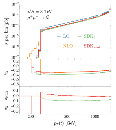
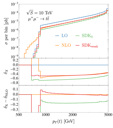
Figure 1: The top quark $p_{T}$ distribution in $\mu^{+}\mu^{-}\to t{\bar{t}}$. The left (right) plot shows results at $\sqrt{S}=3$ TeV ($\sqrt{S}=10$ TeV). The histograms show $\sigma_{\rm LO}$ (blue) and $\sigma_{\rm NLO_{EW}}$ (orange) as well as predictions in the Sudakov approximation in different approaches, i.e., $\sigma_{{\rm SDK_{weak}}}$ (red) and $\sigma_{{\rm SDK_{0}}}$ (green).

We start by looking at the top-quark transverse momentum distribution, $p_{T}(t)$, in $\mu^{+}\mu^{-}\to t\bar{t}$ production. In Fig. 1 we show results for 3 TeV collisions in the left plot and for 10 TeV collisions in the right one. Cuts and the calculation set-up are described in Sec. 3.1. Both plots have the same layout, which will be used also for the other figures of this section and, with more or less small variations, throughout the whole paper. In the following we describe it and we also discuss how to interpret the plots.

Using the same colour code of Ref. Pagani:2021vyk , in the main panel we show LO (blue), $\rm NLO_{EW}$ (orange), ${\rm SDK_{weak}}$ (red), and ${\rm SDK_{0}}$ (green) predictions. In the first inset, we plot the relative corrections induced by such approximations w.r.t. the LO predictions, i.e., the quantities $\delta_{X}$ defined in Eqs. (3.10), (3.14) and more in general (3.26). In such inset it is possible to appreciate the size and the sign of EW corrections, either calculated at exact $\rm NLO_{EW}$ accuracy or via Sudakov approximation(s). Then, in the second inset, we plot the difference $\delta_{X}-\delta_{\rm NLO_{EW}}$ for the two cases $X={\rm SDK_{weak}}$ and $X={\rm SDK_{0}}$ in order to test their accuracy. Rather than the minimisation of this quantity, the validity of the Sudakov approximation consists in having a small constant difference ($|\delta_{X}-\delta_{\rm NLO_{EW}}|\simeq\alpha$) over the full spectrum, i.e. a horizontal line, see also Eqs. (3.18) and (3.19) and text around it. Indeed, ${\cal O}(\alpha)$ contributions are expected to be present, while non-horizontal lines indicate an (at least) logarithmic-enhanced contribution that is not captured. Such contribution may accidentally compensate the ${\cal O}(\alpha)$ constant term and lead to $\delta_{X}-\delta_{\rm NLO_{EW}}\simeq 0$ for particular phase-space regions, but this is not to be regarded as an indication of the validity of the approximation. That said, a large constant difference ($|\delta_{X}-\delta_{\rm NLO_{EW}}|\gg\alpha$), however, also points to logarithms that are not correctly captured. In particular, at a high-energy lepton collider, the direct-production processes studied in this work and characterised by $\sqrt{s}\simeq\sqrt{S}$ may show such effects induced by missing large double logarithms (see Eq. (2.3)) of the form $L(s,M_{W}^{2})$, which are therefore large constants for the full phase-space.

In Fig. 1 we notice that LO, ${\rm SDK_{weak}}$ and ${\rm SDK_{0}}$ predictions quickly drop for $p_{T}(t)\lesssim 250~{}\,\textrm{GeV}$ ($p_{T}(t)\lesssim 800~{}\,\textrm{GeV}$) at 3 TeV (10 TeV) collisions. This is due to the cut on pseudorapidities in (3.3). In that region, only contributions with $\sqrt{s}<\sqrt{S}$ are allowed, and therefore the large suppression from the muon PDF at Bjorken-$x<1$ is the reason for such decrease in the rates. On the contrary, $\rm NLO_{EW}$ predictions, featuring also $2\to 3$ configurations via real photon radiation, can allow for smaller values of $p_{T}(t)$ also with Bjorken-$x\simeq 1$, avoiding the PDF suppression. In that region, which is very much disfavoured w.r.t. the bulk, NLO EW corrections are much larger than the LO predictions and one should in principle also take into account effects from the photon PDF into the muon. Moreover, being dominated by photon real emissions, the comparison of $\rm NLO_{EW}$ predictions with the Sudakov approximation, either ${\rm SDK_{weak}}$ or ${\rm SDK_{0}}$ is meaningless.

For $p_{T}(t)\gtrsim 250~{}\,\textrm{GeV}$ ($p_{T}(t)\gtrsim 800~{}\,\textrm{GeV}$) at 3 TeV (10 TeV) collisions, we can instead discuss for the left (right) plot the features of NLO EW corrections related to the bulk of the distributions and that can be approximated via EWSL. We describe them in the following. First of all, in the first inset we notice that the shape of the EW corrections is very different w.r.t. the typical one observed for $p_{T}$ distributions at hadron colliders, for $pp\to t\bar{t}$ can be found e.g. in Refs. Pagani:2016caq ; Czakon:2017wor . While at hadron colliders, excluding the threshold, $\delta_{\rm NLO_{EW}}$ is negative for $t\bar{t}$ production and from small values at small $p_{T}(t)$ constantly grows in absolute value at large $p_{T}(t)$, here $\delta_{\rm NLO_{EW}}$ is in general large and negative over the full considered spectrum, $\delta_{\rm NLO_{EW}}\simeq-(20$–30%) at 3 TeV and $\delta_{\rm NLO_{EW}}\simeq-(40$–50%) at 10 TeV. Somehow counterintuitively, it slightly decreases in absolute values at large $p_{T}(t)$, the opposite of what is observed at hadron colliders.

The origin of such behaviour has again to be ascribed to the different Bjorken-$x$ dependence of the PDFs of the proton and of the muon. In muon collisions, unlike in the case of the hadron collisions, regardless of the value of $p_{T}(t)$, $s\simeq S$. Thus the $\delta_{\rm DL}$ component proportional to $L(s,M_{W}^{2})$ in Eq. (3.14) is present over the full considered spectrum. In other words, double logarithms are large, especially at 10 TeV, and constant. The single logarithms, as well as the logarithms entering $\delta_{s\rightarrow r_{kl}}$ in Eq. (3.14), conversely, do depend on the kinematic and in particular on the other two Mandelstam variables $t$ and $u$. Overall, they lead to smaller values of $\delta_{{\rm SDK_{weak}}}$, which, as can be clearly seen in the second insets of the two plots of Fig. 1, is a very good approximation of the $\rm NLO_{EW}$ predictions.

Unlike the case of ${\rm SDK_{0}}$, for $p_{T}(t)\gtrsim\sqrt{S}/10$ the ${\rm SDK_{weak}}$ approach can very well approximate the $\rm NLO_{EW}$ result, with a constant discrepancy $\delta_{\rm NLO_{EW}}-\delta_{{\rm SDK_{weak}}}$ of very few percents w.r.t. the LO. This is manifest in the second inset of the two plots of Fig. 1, where it can also be seen that in the case of ${\rm SDK_{0}}$ this discrepancy is instead of the order $\delta_{\rm NLO_{EW}}-\delta_{{\rm SDK_{0}}}\simeq-(5$–10%) at 3 TeV and $\delta_{\rm NLO_{EW}}-\delta_{{\rm SDK_{0}}}\simeq-(15$–20%) at 10 TeV. Thus, $\delta_{\rm NLO_{EW}}-\delta_{{\rm SDK_{0}}}$ is much larger in absolute value than $\delta_{\rm NLO_{EW}}-\delta_{{\rm SDK_{weak}}}$, and it depends much more on the value of $p_{T}(t)$ and especially on the energy of the collider. They are all clear signs that both double and single EWSL logarithms are not correctly captured by the ${\rm SDK_{0}}$ scheme, unlike the case of the ${\rm SDK_{weak}}$ one.

In the region just above $p_{T}(t)\simeq 250~{}\,\textrm{GeV}$ ($p_{T}(t)\simeq 800~{}\,\textrm{GeV}$) at 3 TeV (10 TeV) collisions another effect is entering, slightly altering the agreement of $\delta_{{\rm SDK_{weak}}}$ with $\delta_{\rm NLO_{EW}}$, and similarly for the $\delta_{{\rm SDK_{0}}}$ case. At NLO, the real emission collinear to the initial state can alter the kinematic and therefore has an impact on the accuracy of the Sudakov approximation. On the one hand, even with Bjorken-$x\simeq 1$ for the muon PDF, we can have a smaller invariant mass $m(t\bar{t})$ for the $t\bar{t}$ pair, allowing for smaller values of $p_{T}(t)$ also with the cuts in (3.3). On the other hand, the boost from the recoil against the photon emission can lead to more peripheral top quarks, which cannot pass therefore the cuts. In conclusion, it is not surprising that such effects are arising close to cuts that LO, ${\rm SDK_{weak}}$ and ${\rm SDK_{0}}$ predictions cannot pass, unless Bjorken-$x\lesssim 1$, but that $\rm NLO_{EW}$ predictions can instead pass also with Bjorken-$x\simeq 1$. Moreover, in the case of 3 TeV collisions, in this region $p_{T}(t)$ is only mildly larger than $M_{W}$, so non-negligible power corrections of the form $M_{W}^{2}/t$ or $M_{W}^{2}/u$ cannot be excluded.

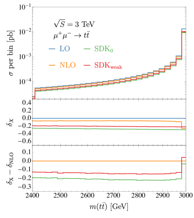
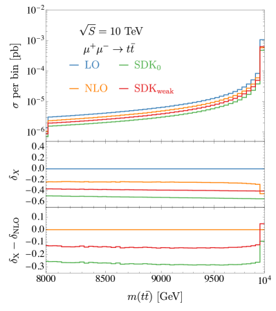
Figure 2: Same as Fig. 1, for the $m(t{\bar{t}})$ distribution in $\mu^{+}\mu^{-}\to t{\bar{t}}$.

Many of the points of the discussion of the $p_{T}(t)$ plots of Fig. 1 can be better understood by looking at the top-quark invariant mass distribution $m(t\bar{t})$, which we show in Fig. 2. All the contributions from LO, ${\rm SDK_{weak}}$ and ${\rm SDK_{0}}$ predictions at Bjorken-$x\simeq 1$ enter the last bin at $m(t\bar{t})\simeq\sqrt{S}$, while in the case of $\rm NLO_{EW}$ predictions they can contribute over the full spectrum. This is the reason why, besides in the rightmost bin, the agreement between the $\rm NLO_{EW}$ predictions and their Sudakov approximation is not good, regardless of the scheme choice. We remind the reader that we cluster the photon in the real emission with the top (anti)quark if they are collinear such that, for this kind of contributions, $m(t\bar{t})\simeq S$ also in the presence of very hard photons.

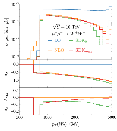
Figure 3: Same as Fig. 1, for the $p_{T}(W_{2})$ distribution in $\mu^{+}\mu^{-}\to W^{+}W^{-}$.

We move now to the case of a different process, the $\mu^{+}\mu^{-}\to W^{+}W^{-}$ production. In Fig. 3 we show the distribution of the transverse momentum of the softest $W$ boson, $p_{T}(W_{2})$. Many features are common to the case of the $\mu^{+}\mu^{-}\to t\bar{t}$ production process in Fig. 1. In the following, we highlight the differences rather than the similarities.

At variance with the $\mu^{+}\mu^{-}\to t\bar{t}$ production process, the tree-level amplitude of $\mu^{+}\mu^{-}\to W^{+}W^{-}$ production features $t$- and $u$-channel diagrams and consequently LO predictions are much less suppressed moving from large to small values of $p_{T}(W_{2})$ w.r.t. what is observed in in Fig. 1. Thus, the distributions are much flatter, excluding again the region $p_{T}(W_{2})\lesssim 250~{}\,\textrm{GeV}$ ($p_{T}(W_{2})\lesssim 800~{}\,\textrm{GeV}$) at 3 TeV (10 TeV) collisions, which is affected by the rapidity cuts in (3.3).

The EW corrections, exact ($\rm NLO_{EW}$) or in Sudakov approximation (${\rm SDK_{weak}}$ or ${\rm SDK_{0}}$) are much larger in the case of $W^{+}W^{-}$, cf. Fig. 1 and Fig. 3. At 10 TeV the EW corrections are so large that at large $p_{T}(W_{2})$ values, where the cross section is maximal, $\delta_{\rm NLO_{EW}}<-100\%$ and therefore the $\rm NLO_{EW}$ prediction becomes negative. This is a clear sign of the necessity of resumming the large EWSL and we will return to this aspect in Sec. 4.2. Larger corrections are not surprising, since the couplings of the $W$ bosons with EW gauge bosons are larger w.r.t. the top quarks. The shape of $\delta_{\rm NLO_{EW}}$ is also different w.r.t. $t\bar{t}$ direct production. First, $\delta_{\rm NLO_{EW}}$ is much less flat, denoting a larger contribution from single logarithms, as well as the logarithms entering $\delta_{s\rightarrow r_{kl}}$ in Eq. (3.14). Second, for larger values of $p_{T}(W_{2})$, $\delta_{\rm NLO_{EW}}$ grows in absolute value, similarly to the typical shape observed at hadron colliders.

Moving to the comparison of the Sudakov approximation against the exact NLO EW corrections, the overall pattern is quite similar with a few differences w.r.t. Fig. 1. It is impressive how at large $p_{T}(W_{2})$ values exact NLO EW corrections can be approximated at the level of ${\cal O}(1\%)$ of the LO by the ${\rm SDK_{weak}}$ predictions (see second inset) when the corrections themselves are of ${\cal O}(100\%)$ of the LO for 10 TeV collisions (see first inset). The same argument does not apply to the ${\rm SDK_{0}}$ predictions. Considering smaller values of $p_{T}(W_{2})$, we see that the agreement of ${\rm SDK_{weak}}$ predictions and the exact $\rm NLO_{EW}$ is less good w.r.t. the case of $t\bar{t}$ production. To the best of our understanding, this is due to the logarithms involving the ratios of invariants as $|t|/s$ or $|u|/s$. The $\delta_{s\rightarrow r_{kl}}$ improves a lot the approximation of these contributions, see the discussion in the next section, but as already said it may miss some of such logarithms. In the case of $W^{+}W^{-}$ production, we see non-negligible effects due to these logarithms that are correctly captured only by $\rm NLO_{EW}$ predictions.

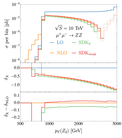
Figure 4: Same as Fig. 1, for the $p_{T}(Z_{2})$ distribution in $\mu^{+}\mu^{-}\to ZZ$.

In Fig. 4 we show the analogous distribution of Fig. 3 for $\mu^{+}\mu^{-}\to ZZ$ production, $p_{T}(Z_{2})$. Here NLO EW corrections are even larger in absolute value than in the case of $WW$ production. Still, the ${\rm SDK_{weak}}$ approximation is again accurate at the level of ${\cal O}(1\%)$ of the LO. Since the particles in the final state are not electrically charged the choice of the ${\rm SDK_{weak}}$ scheme is not returning results that are very different w.r.t. the ${\rm SDK_{0}}$ one, especially for what concerns the shape of distributions, since the photon exchange between the initial and final state is not possible. Still, the muons in the initial state are electrically charged, so there are double logarithms of the form $L(s,M_{W}^{2})\simeq L(S,M_{W}^{2})$ that are treated differently in the two schemes and lead, especially at 10 TeV, to a constant difference between $\delta_{{\rm SDK_{weak}}}$ and $\delta_{{\rm SDK_{0}}}$, degrading the agreement with $\delta_{\rm NLO_{EW}}$ for the latter.

We have also considered the $m(W^{+}W^{-})$ and $m(ZZ)$ distributions, which we do not show for brevity here. Similar to the case of $t\bar{t}$ production we see a large suppression due to PDFs for $m(W^{+}W^{-}),m(ZZ)<\sqrt{S}$. In the case of $m(W^{+}W^{-})$ we see a similar pattern, although less dramatic when moving from the last bin, $m(W^{+}W^{-})\simeq\sqrt{S}$, to the others, $m(W^{+}W^{-})<\sqrt{S}$. In the case of $ZZ$ production, we do not cluster photons with $Z$ bosons, since from them no photon emissions leading to EWSL are possible. For the same reason, we do not see a discontinuity from the rightmost bin with $m(ZZ)\simeq\sqrt{S}$ to the other ones with $m(ZZ)<\sqrt{S}$. For both processes, the contributions from hard photons collinear to the initial-state muons are subtracted by PDF counterterms in the $\rm NLO_{EW}$ predictions. These are the same double logarithms mentioned in the previous paragraph and this subtraction is correctly taken into account by the ${\rm SDK_{weak}}$ scheme, which indeed exhibits for the $m(ZZ)$ distributions an ${\cal O}(1\%)$ of the LO accuracy over the full spectrum.

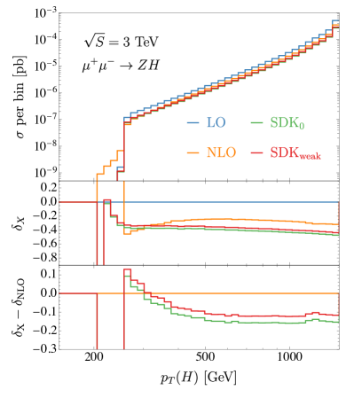
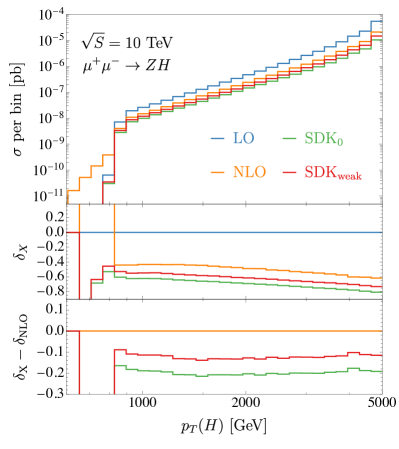
Figure 5: Same as Fig. 1, for the Higgs boson $p_{T}$ distribution in $\mu^{+}\mu^{-}\to ZH$.

Finally, in Fig. 5 we show the transverse-momentum distribution for the Higgs boson in $\mu^{+}\mu^{-}\to ZH$ production, $p_{T}(H)$. Similarly to the case of $t\bar{t}$ production in Fig. 1, we observe a much less flat LO prediction w.r.t. the case of $WW$ and $ZZ$ production. As in the case of $t\bar{t}$ production, and unlike $WW$ and $ZZ$, the tree-level amplitude features only an $s$-channel diagram. As in $t\bar{t}$ production, and even more, $\delta_{\rm NLO_{EW}}$ is quite flat over the full spectrum. We also observe that the difference $\delta_{{\rm SDK_{weak}}}-\delta_{\rm NLO_{EW}}$ is larger, of the order of $10\%$ both for 3 and 10 TeV collisions. Instead, in the case of $\delta_{{\rm SDK_{0}}}-\delta_{\rm NLO_{EW}}$, such difference is of the order of $15\%$ at 3 TeV and $20\%$ at 10 TeV. Thus, the accuracy of $\delta_{{\rm SDK_{0}}}$ is not only worse but also energy-dependent. To the best of our understanding, the $\mu^{+}\mu^{-}\to ZH$ has large non-logarithmic-enhanced contributions at ${\cal O}(\alpha)$ and on top of that the $\delta_{{\rm SDK_{0}}}$ wrongly approximates the double logarithms of the form $L(s,M_{W}^{2})\simeq L(S,M_{W}^{2})$ from the photon exchange among the muons in the initial state. Notice that the difference $\delta_{{\rm SDK_{weak}}}-\delta_{{\rm SDK_{0}}}$ is the same observed, both at 3 and 10 TeV, for $\mu^{+}\mu^{-}\to ZZ$ production in Fig. 4, for which the same argument was presented.

We have also calculated and analysed the $m(ZH)$ distribution. The situation is similar to the one observed for the $m(ZZ)$ distribution, but the $\delta_{{\rm SDK_{weak}}}-\delta_{\rm NLO_{EW}}$ remains constant at the order of $10\%$ as discussed for the $p_{T}(H)$ distribution.

4.1.2 Importance of logarithms involving ratios of invariants

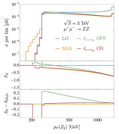
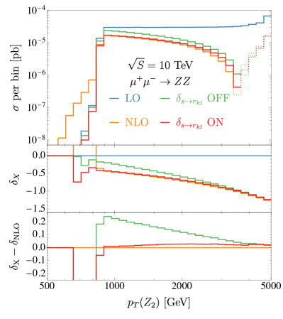
Figure 6: The $p_{T}(Z_{2})$ distribution in $\mu^{+}\mu^{-}\to ZZ$. The left (right) plot shows results at $\sqrt{S}=3$ TeV ($\sqrt{S}=10$ TeV). The histograms show $\sigma_{\rm LO}$ (blue) and $\sigma_{\rm NLO_{EW}}$ (orange) as well as predictions in the Sudakov approximation in the ${\rm SDK_{weak}}$ approach including (red) or neglecting (green) the term $\delta_{s\rightarrow r_{kl}}$.

In this section, we discuss the relevance of the term $\delta_{s\rightarrow r_{kl}}$ entering Eq. (3.14) and introduced in Ref. Pagani:2021vyk . As already explained, this term accounts for (large part of the) logarithms of the form $L(|r_{kl}|,s)$ and $l(|r_{kl}|,s)$, see Eq. (2.3). Whenever a large hierarchy among invariants is present, these logarithms become numerically relevant. For processes as those studied in this work, where $\sqrt{s}\simeq\sqrt{S}=3$ or 10 TeV but transverse momenta can be a few hundred GeV’s, $\delta_{s\rightarrow r_{kl}}$ is expected to be very relevant. One should notice that invariants can be small(large) due to small(large) angles among two particles and therefore angular distributions are very sensitive to these logarithms.

In order to minimise the overlap with the effects discussed in the previous section, ${\rm SDK_{weak}}$ vs. ${\rm SDK_{0}}$, we consider final states with only neutrally charged particles, in particular: the $ZZ$, $ZH$, $ZZZ$, and $ZZH$ production processes. The layout of the plots in this section is very similar to those shown in the previous section. The only difference w.r.t. them is that we show here ${\rm SDK_{weak}}$ as defined in Eq. (3.14) (again displayed as a solid red line) and the same quantity where we set $\delta_{s\rightarrow r_{kl}}=0$ (solid green line) in the aforementioned equation.

We start by showing again the same observables considered for $ZZ$ and $ZH$ production in the previous section, $p_{T}(Z_{2})$ for $ZZ$ production in Fig. 6 and $p_{T}(H)$ for $ZH$ production in Fig. 7. In Fig. 6 we clearly see that for $p_{T}(Z_{2})\gtrsim 250~{}\,\textrm{GeV}$ ($p_{T}(Z_{2})\gtrsim 800~{}\,\textrm{GeV}$) at 3 TeV (10 TeV) collisions, the very good accuracy of the ${\rm SDK_{weak}}$ prediction ($\delta_{{\rm SDK_{weak}}}-\delta_{\rm NLO_{EW}}$ constant and of ${\cal O}(1\%)$) is much degraded when $\delta_{s\rightarrow r_{kl}}=0$, i.e. the green line in the second inset. Indeed, while at large $p_{T}(Z_{2})$ we see $\delta_{{\rm SDK_{weak}}}-\delta_{\rm NLO_{EW}}\simeq 1\%$, at smaller values, $p_{T}(Z_{2})\simeq 250~{}\,\textrm{GeV}$ ($p_{T}(Z_{2})\simeq 800~{}\,\textrm{GeV}$) at 3 TeV (10 TeV), we notice that $\delta_{{\rm SDK_{weak}}}-\delta_{\rm NLO_{EW}}\simeq 30\%$. Since the $p_{T}(Z_{2})$ distribution is quite flat, this discrepancy at small $p_{T}(Z_{2})$ has an effect also at the level of the total cross section; setting $\delta_{s\rightarrow r_{kl}}=0$ we find that, for both 3 and 10 TeV, with the cuts considered $\delta_{{\rm SDK_{weak}}}-\delta_{\rm NLO_{EW}}\simeq 10\%$ also for the total cross section. A similar (quite constant) discrepancy is observed in the $m(ZZ)$ distribution, too. These results are clearly dependent on the cuts in $\eqref{eq:cuts}$, in particular the one on the pseudorapidity of the $Z$ bosons. Setting $\delta_{s\rightarrow r_{kl}}=0$ logarithms of the form, e.g., $L(|t|,s)$ are omitted and, in the proximity of the pseudorapidity cuts, such logarithms are of the same order for both the 3 and 10 TeV results.

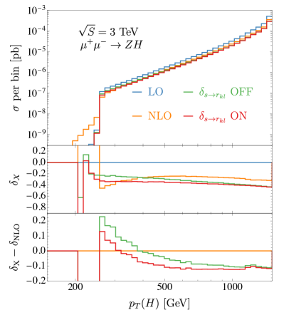
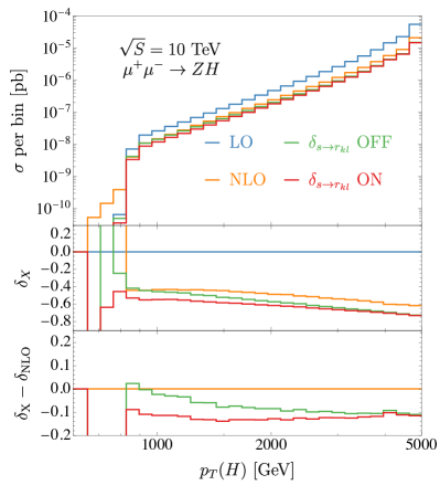
Figure 7: Same as Fig. 6, for the $H$ boson $p_{T}$ distribution in $\mu^{+}\mu^{-}\to ZH$.

The case of $p_{T}(H)$ distribution in $ZH$ production, Fig. 7, shows a very similar pattern at the differential level, although the impact of $\delta_{s\rightarrow r_{kl}}$ is smaller. However, since the $p_{T}(H)$ distribution is much less flat, at the inclusive level also with $\delta_{s\rightarrow r_{kl}}=0$ a good accuracy for the ${\rm SDK_{weak}}$ prediction is present. It is interesting to note that for small values of $p_{T}(H)$ at 10 TeV the case with $\delta_{s\rightarrow r_{kl}}=0$ yields smaller values of $\delta_{{\rm SDK_{weak}}}-\delta_{\rm NLO_{EW}}$. As said at the beginning of the previous section, this is not per se a sign of better accuracy. Indeed this effect is due to missing logarithms among invariants that accidentally compensate the large non-logarithmically enhanced ${\cal O}(\alpha)$ component already discussed in the case of Fig. 5.

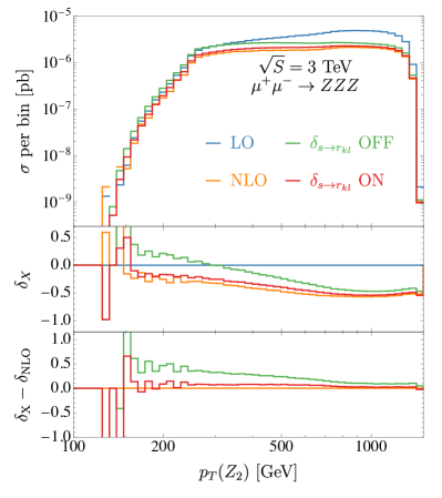
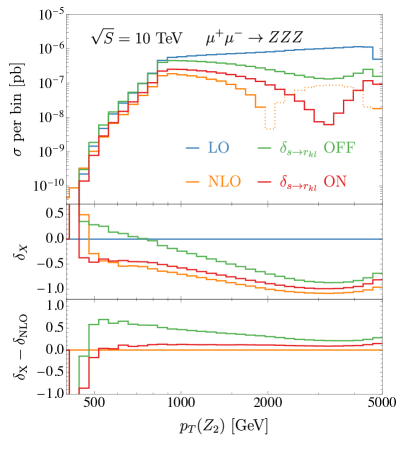
Figure 8: Same as Fig. 6, for the $p_{T}(Z_{2})$ distribution in $\mu^{+}\mu^{-}\to ZZZ$.

We move now to the case of $2\to 3$ processes, $ZZZ$, and $ZZH$ production, for which more independent kinematic invariants are present. In Fig. 8 we show the transverse-momentum distribution of the second-hardest $Z$ boson, $p_{T}(Z_{2})$. As can be noticed, EW corrections are very large ($\delta_{\rm NLO_{EW}}<-100\%$ at 10 TeV in the bulk of the distribution), and the ${\rm SDK_{weak}}$ approximation (solid line) is able to capture correctly the kinematic dependence with a constant discrepancy $\delta_{{\rm SDK_{weak}}}-\delta_{\rm NLO_{EW}}\simeq 10\%$. On the contrary, setting $\delta_{s\rightarrow r_{kl}}=0$ (dashed line), we observe a constant growth of $\delta_{{\rm SDK_{weak}}}-\delta_{\rm NLO_{EW}}$ moving to small $p_{T}(Z_{2})$ values.

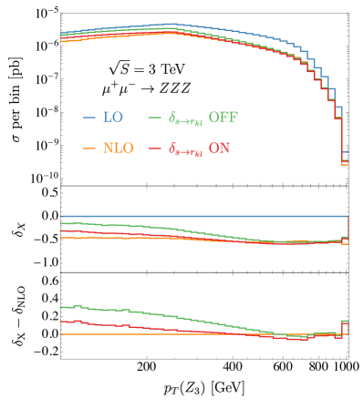
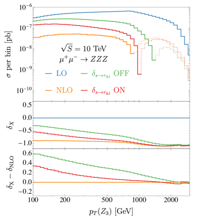
Figure 9: Same as Fig. 6, for the $p_{T}(Z_{3})$ distribution in $\mu^{+}\mu^{-}\to ZZZ$.

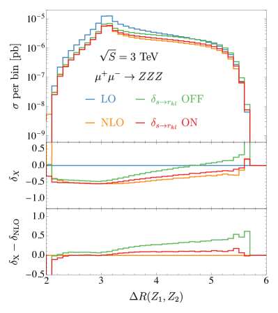
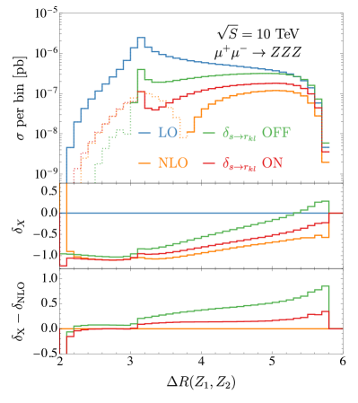
Figure 10: Same as Fig. 6, for the $\Delta R(Z_{1},Z_{2})$ distribution in $\mu^{+}\mu^{-}\to ZZZ$.

To the best of our understanding, this $10\%$ discrepancy is not due to a large non-logarithmically enhanced ${\cal O}(\alpha)$ component, as in the case of $ZH$ distributions, but to large logarithms that the ${\rm SDK_{weak}}$ scheme is not able to capture even retaining the $\delta_{s\rightarrow r_{kl}}$ term. This can better understood by looking at the $p_{T}(Z_{3})$ distribution, the $p_{T}$ of the softest $Z$ boson, in Fig. 9 and the $\Delta R(Z_{1},Z_{2})$ distribution in Fig. 10, in particular at 10 TeV. First we observe that for very large $p_{T}(Z_{3})$, meaning all $Z$ bosons that are hard and so all the invariants that are large, $\delta_{{\rm SDK_{weak}}}-\delta_{\rm NLO_{EW}}\to 0$, while the same quantity constantly grows in the opposite direction. Second, for $\Delta R(Z_{1},Z_{2})\lesssim\pi$, $\delta_{{\rm SDK_{weak}}}-\delta_{\rm NLO_{EW}}\simeq 0$, while for $\Delta R(Z_{1},Z_{2})\gtrsim\pi$ the same quantity jumps to $\sim 10\%$ and remains constant up to $\Delta R(Z_{1},Z_{2})\simeq 5$. The dominant kinematic configuration is $Z_{1}$ and $Z_{2}$ that are almost back-to-back, i.e. $\Delta R(Z_{1},Z_{2})\simeq\pi$. The region $\Delta R(Z_{1},Z_{2})\lesssim\pi$ is dominated by large values of $p_{T}(Z_{3})$, which therefore are correlated and both show $\delta_{{\rm SDK_{weak}}}-\delta_{\rm NLO_{EW}}\simeq 0$. Instead, in the region $\Delta R(Z_{1},Z_{2})\gtrsim\pi$ large contributions from the $\rm NLO_{EW}$ prediction originate from the $ZZZ\gamma$ final state, which allows a further recoil and enhances $|\eta(Z_{1})-\eta(Z_{2})|$ and in turn $\Delta R(Z_{1},Z_{2})$. This dynamics is only captured by the $\rm NLO_{EW}$ prediction. Another peculiar behaviour is observed in the first bins of the distribution, where the EWSL prediction departs from the NLO EW. This is due to the fact that, in a Born-like kinematics, the first bin can be filled only when all $Z$ bosons have equal transverse momentum. Photon radiation, captured only by the NLO EW prediction, lifts such a constraint, and can thus enhance this region All in all, for this process, the inclusion of $\delta_{s\rightarrow r_{kl}}$ is crucial for improving the approximation. Nevertheless, non-negligible effects are not captured.

Figure 11: Same as Fig. 6, for the $\Delta R(Z_{1},Z_{2})$ distribution in $\mu^{+}\mu^{-}\to ZZH$.

In Fig. 11 we show the $\Delta R(Z_{1},Z_{2})$ distribution for $ZZH$ production. In this case, the situation is a combination of effects observed already for the $ZH$ and $ZZZ$ processes. To the best of our understanding, there are both logarithms that cannot be correctly captured, as in $ZZZ$, and a large non-logarithmically enhanced ${\cal O}(\alpha)$ component.

In conclusion, considering also other distributions for other processes that we have calculated but not shown in the paper, the quantity $\delta_{s\rightarrow r_{kl}}$ in general improves the approximation of the EWSL, but additional contributions present at $\rm NLO_{EW}$ accuracy can be omitted. For precise predictions, such contributions cannot be neglected.

4.1.3 The case of numerically large contributions from mass-suppressed terms.

As clearly stated in Refs. Denner:2000jv ; Denner:2001gw , the DP algorithm assumes that the helicity configuration considered is not mass suppressed, i.e., as said in Sec. 2.2.1, that it scales as ${\cal{M}}\propto s^{\frac{2-n}{2}}$ for a $2\to n$ process. In general, in the SM, at least one of the helicity configurations of the processes considered is typically not mass suppressed and therefore at high energies is very enhanced w.r.t. the other ones. For this reason, even blindly applying the DP algorithm to all helicity configurations, regardless if they are or are not mass-suppressed, the prediction for the sum over the polarisations is consistent, namely it corresponds to the high-energy limit $M_{W}^{2}/s\to 0$. In other words, even if the algorithm returns wrong results for the mass-suppressed helicity configurations, they are so suppressed that the relative impact in the sum over the helicity configurations is completely negligible. However, it is known that there can be processes where none of the helicity configurations are not mass-suppressed, such as Higgs VBF production. For such cases, the DP algorithm is known to no be working.

In this section, we give an example that is a bit more subtle. We consider the case of the $\mu^{+}\mu^{-}\to ZHH$ production process, which does feature helicity configurations that are not mass suppressed, but that in part of the phase space are not numerically the dominant ones. Thus, the DP algorithm leads to wrong results for the evaluation of high-energy limit $M_{W}^{2}/s\to 0$ of the EW corrections.

Figure 12: The $m(HH)$ distribution in $\mu^{+}\mu^{-}\to ZHH$. The left (right) panel shows results at $\sqrt{S}=3$ TeV ($\sqrt{S}=10$ TeV). The histograms show $\sigma_{\rm LO}$ (blue), $\sigma_{\rm NLO_{EW}}$ (orange) and $\sigma_{{\rm SDK_{weak}}}$.

Figure 13: Same as Fig. 12, for the $Z$ boson $p_{T}$ distribution in $\mu^{+}\mu^{-}\to ZHH$.

In Fig. 12 we show the invariant-mass distribution of the $HH$ pair, $m(HH)$, while in Fig. 13 we show the $p_{T}(Z)$ distribution. All plots have the same layout used already in the previous sections, but we show only ${\rm SDK_{weak}}$ results for the Sudakov approximation. It is manifest that for low values of $m(HH)$, the ${\rm SDK_{weak}}$ prediction is completely off from the exact $\rm NLO_{EW}$ one: $|\delta_{{\rm SDK_{weak}}}-\delta_{\rm NLO_{EW}}|\gg 100\%$. At first, one may think that even including the $\delta_{s\rightarrow r_{kl}}$ contribution large logarithms of the form $L(m^{2}(HH),s)$ are not correctly captured, but this bad agreement between ${\rm SDK_{weak}}$ and $\rm NLO_{EW}$ starts to appear already at quite large $m(HH)$ values. The origin is different and we explain it in the following.

Since $\sqrt{s}\simeq\sqrt{S}$, small $m(HH)$ values are related to configurations where a hard $Z$ boson recoils against a $HH$ pair, with the two Higgs bosons hard and collinear. Indeed, the same features present at low $m(HH)$ in Fig. 12 are visible also in Fig. 13 at large $p_{T}(Z)$. For $m(HH)\ll\sqrt{s}$, the tree-level diagram featuring the $\mu^{+}\mu^{-}\to ZH^{*}(H^{*}\to HH)$ topology leads to numerically large contributions that formally are mass suppressed. Indeed, considering simply the $H^{*}\to HH$ part of the amplitude, it leads to a contribution of order

$${\cal{M}}(H^{*}\to HH)\propto\frac{v\lambda}{\left(m(HH)\right)^{2}-M_{H}^{2}}\sim\frac{M_{H}^{2}}{v\left(m(HH)\right)^{2}}\left[1+{\cal O}\left(\frac{M_{H}^{2}}{\left(m(HH)\right)^{2}}\right)\right]\,,$$ (4.1)

which is not numerically small but it is mass suppressed. Indeed if it were not mass suppressed it would have scaled as $1/m(HH)$, consistent with the scaling ${\cal{M}}\propto s^{\frac{2-n}{2}}$ for a $2\to n$ process, or equivalently for a process $n\to 2$ where here $n=1$. In this scenario, the DP algorithm is not expected to work and indeed it does not.

The most important point to keep in mind is that NLO EW corrections are not small, but they cannot be approximated via the DP algorithm. Even more surprisingly (at least before understanding the underlying dynamics), the ${\rm SDK_{weak}}$ works well for small $p_{T}(Z)$ values but not for large values, which is the opposite of what one would expect. Similar situations may manifest also for BSM scenarios, where rates may be much larger than the SM process considered here. This is a clear sign of the necessity of exact $\rm NLO_{EW}$ corrections also in BSM studies for the physics at the muon collider.

4.2 Beyond NLO EW: the relevance of resummation

Figure 14: The top quark $p_{T}$ distribution in $\mu^{+}\mu^{-}\to t{\bar{t}}$. The left (right) panel shows results at $\sqrt{S}=3$ TeV ($\sqrt{S}=10$ TeV). The histograms show $\sigma_{\rm LO}$ (blue), $\sigma_{\rm NLO_{EW}}$ (orange), the EWSL prediction in the ${\rm SDK_{weak}}$ approach and $\sigma_{\rm EXP_{EW}}$ (black dashed), which corresponds to the approximate resummation of EW corrections.

In this section, we investigate if and when the resummation of EWSL of higher order, i.e. of ${\cal O}(\alpha^{n})$ with $n>1$, is expected to be relevant. We do not perform actual resummation, rather we approximate it via exponentiation of the ${\rm SDK_{weak}}$ result and match it additively to the $\rm NLO_{EW}$ prediction.. We have dubbed such approximation as $\rm EXP_{EW}$ and it has been properly defined in Eq. (3.20). We show plots similar to those of Sec. 4.1, showing also the $\rm EXP_{EW}$ predictions and in the first inset the $\delta_{\rm EXP_{EW}}$ (black dashed). In the second inset we show $\delta_{\rm EXP_{EW}}-\delta_{\rm NLO_{EW}}$, in order to emphasise the expected impact of EWSL of higher order and possibly the relevance of resumming them. The term $\delta_{\rm EXP_{EW}}-\delta_{\rm NLO_{EW}}$, multiplied by -1, is the finite part of not EWSL origin that would not enter the resummation procedure.

We start showing again the $p_{T}(t)$ in $t\bar{t}$ production, as in Fig. 1. For this observable, the EWSL of higher order are expected to be relevant for precision at ${\cal O}(1\%)$ at 3 TeV and at ${\cal O}(10\%)$ at 10 TeV, as can be seen in Fig. 14 by the difference between the $\delta_{\rm EXP_{EW}}$ and $\delta_{\rm NLO_{EW}}$ relative corrections. However, resummation appears not to be mandatory for obtaining phenomenologically sensible results at 3 TeV. Moreover, it is of the same order as the non-logarithmic enhanced contributions at $\rm NLO_{EW}$ accuracy.

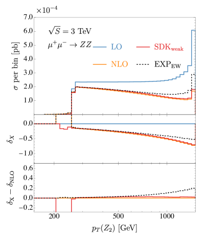
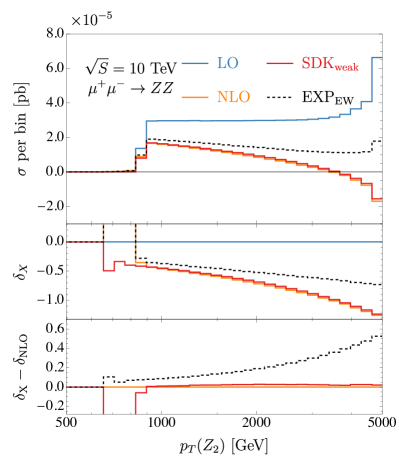
Figure 15: Same as Fig. 14, for $p_{T}(Z_{2})$ distribution in $\mu^{+}\mu^{-}\to ZZ$

The case of $p_{T}(Z_{2})$ in $ZZ$ production, already considered in Fig. 4, is different. As can be seen in Fig. 15, at 3 TeV EWSL of higher order are expected to be relevant for precision at ${\cal O}(10\%)$, they are much larger than what has been observed in Fig. 14 at the same energy for $p_{T}(t)$ in $t\bar{t}$ production, but still not mandatory for phenomenologically sensible results. The situation is completely different at 10 TeV. The EW corrections are so large that the prediction at $\rm NLO_{EW}$ accuracy is even negative for large values of $p_{T}(Z_{2})$, therefore it is non-physical. The resummation in this case is not concerning only precision studies; it is the only possible way of obtaining phenomenologically sensible results. We observed a similar pattern in $WW$ production, which we do not explicitly show for brevity.

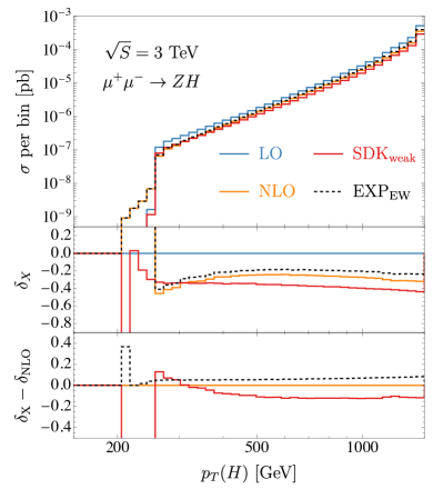
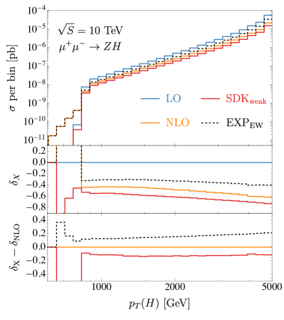
Figure 16: Same as Fig. 14, for the Higgs boson $p_{T}$ distribution in $\mu^{+}\mu^{-}\to ZH$

The case of $ZH$ production, already shown in Fig. 5, is a bit different. As can be seen in Fig. 16, EWSL of higher order are expected to be of ${\cal O}(10\%)$ at 3 TeV and ${\cal O}(20\%)$ at 10 TeV. Such effects are both of the same order of the $\delta_{{\rm SDK_{weak}}}-\delta_{\rm NLO_{EW}}$ result discussed for Fig. 5 and also visible in the second insets of the plots of Fig. 5. If a precision at ${\cal O}(10\%)$ is required, both the resummation of the EWSL and the matching with the exact $\rm NLO_{EW}$ predictions are expected to be relevant.

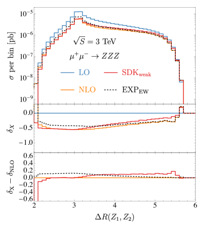
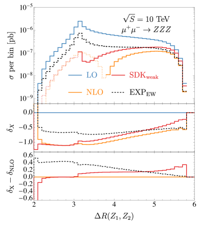
Figure 17: Same as Fig. 14, for the $\Delta R(Z_{1},Z_{2})$ distribution in $\mu^{+}\mu^{-}\to ZZZ$.

As a last example, before giving our conclusion on the relevance of resummation of EWSL for muon-collider physics, we show the case of $\Delta R(Z_{1},Z_{2})$ in $ZZZ$ production, already shown in Fig. 10. In Fig. 17 we see that again at 3 TeV resummation is relevant only for ${\cal O}(10\%)$ accuracy studies, while at 10 TeV resummation is mandatory for having positive cross sections and phenomenologically sensible results. It is also interesting to notice that, for both energies, the range where resummation is of particular relevance ($\Delta R(Z_{1},Z_{2})\lesssim\pi$) is the opposite of the one ($\Delta R(Z_{1},Z_{2})\gtrsim\pi$) of the range where the difference between $\delta_{\rm NLO_{EW}}$ and $\delta_{{\rm SDK_{weak}}}$ are not negligible.

In conclusion, we observe that at 3 TeV resummation is certainly relevant for precise predictions, but it is not mandatory for performing phenomenological studies. The $\rm NLO_{EW}$ predictions, or equivalently the Sudakov approximation (including $\delta_{s\rightarrow r_{kl}}$ and using the ${\rm SDK_{weak}}$ scheme as discussed in Sec. 4.1), can be sufficient. When precision is the target, other effects not considered in this paper should be also considered: NNLO EW corrections, the accuracy of PDFs, the renormalisation scheme as well as the resummation of multiple-photon emissions. In that direction, several studies and technological advancements are desirable in view of the muon-collider physics program. We want to stress that we considered here processes featuring the $Z$ bosons in the final state, which are related to the largest EW corrections at high energies. Thus, it is difficult that other processes may exhibit even larger effects.

At 10 TeV the picture is different. Some processes, as shown in the case of $t\bar{t}$ production, are not expected to lead to extremely large corrections and so also at this energy resummation is necessary only for precision. Other processes instead require the resummation of EWSL. We stress again that we did not perform actual resummation, we approximated it via simple exponentiation. However, our results call for the necessity of performing (at least) Next-to-Leading-Logarithmic (NLL) resummation in muon-collider studies for physics at 10 TeV. We stress that, as already discussed in Sec. 4.1, for these processes and given the Bjorken-$x$ dependence of the muon PDF, since $s\simeq S$ if $\delta_{\rm NLO_{EW}}$ is not a constant, that is a clear sign that not only the LL (the double logarithms in $\delta_{\rm NLO_{EW}}$) but also the NLL (the single logarithms in $\delta_{\rm NLO_{EW}}$) are relevant; LL resummation is not sufficient. That said, it appears clear that the case of $t\bar{t}$ production is not unique, e.g. we observed the same pattern in $e^{+}e^{-}$ production. Intermediate configurations between this case and the processes featuring $Z$ bosons and very large corrections are clearly possible. In other words, case-by-case studies are necessary and the automation of NLL resummation of EWSL would be very helpful. Finally, the same considerations for 3 TeV collisions concerning precision are clearly also valid for 10 TeV collisions.

4.3 Heavy Boson Radiation (HBR)

One of the widespread assumptions about a high energy muon collider is that soft and/or collinear splittings involving heavy weak bosons ($W$, $Z$ and $H$) will lead to ${\cal O}(1)$ corrections, similarly to the case of QCD at the LHC, see e.g. Han:2020uid ; Han:2021lnp . On the one hand, this implies that a muon collider can be treated as a EW boson collider, Costantini:2020stv ; Buttazzo:2020uzc ; Han:2020uid ; Han:2021lnp ; Ruiz:2021tdt ; AlAli:2021let ; Accettura:2023ked leading to very large cross sections for VBF processes. On the other hand, the emission of $W,Z$ and possibly $H$ bosons, i.e., what has been dubbed in this work as HBR, is in general expected to lead to large effects or even becoming dominant w.r.t. the case with no radiation. This dynamics has already been studied in detail in particular scenarios, e.g. showing how it can help to gain sensitivity to new short-distance physical laws Chen:2022msz .

In this section, we investigate if ${\cal O}(1)$ corrections from HBR is really a ubiquitous effect. To this purpose, we consider direct production processes as those already studied in the previous sections. Moreover, we compare and combine the relative corrections induced by the HBR, i.e. the quantity $\delta_{\rm HBR}$ defined in Eq. (3.11), and the relative NLO EW corrections ($\delta_{\rm NLO_{EW}}$), since both of them are of ${\cal O}(\alpha)$ w.r.t. the inclusive production process considered. In doing so we also inspect the degree of cancellation between $\delta_{\rm NLO_{EW}}$, which is typically negative, and $\delta_{\rm HBR}$, which is positive by definition.

In Sec. 4.3.1 we consider the $\mu^{+}\mu^{-}\to F$ processes $F=t\bar{t},\,W^{+}W^{-}$ and the effects of the additional HBR with $B=H,Z$. In Sec. 4.3.2 instead we consider the case of EW jets ($j_{\rm EW}$), where $j_{\rm EW}$ is emerging from the clustering of $V=W,Z$. Details on the clustering of the $j_{\rm EW}$’s themselves and of the HBR with the particles in the final state $F$ are described in Sec. 3.1 and we will not repeat them through the next two sections.

4.3.1 Final states: $t\bar{t}$, $W^{+}W^{-}$

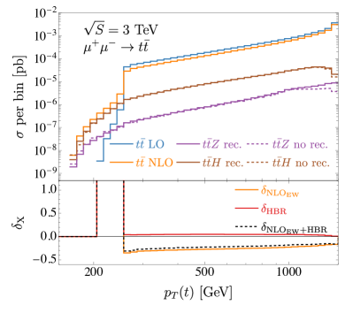
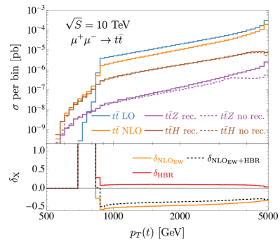
Figure 18: The top quark $p_{T}$ distribution in $\mu^{+}\mu^{-}\to t{\bar{t}}$. The left (right) plot shows results at $\sqrt{S}=3$ TeV ($\sqrt{S}=10$ TeV). The histograms show $\sigma_{\rm LO}$ (blue), $\sigma_{\rm NLO_{EW}}$ (orange), the HBR contribution due to the $Z$ (violet) and to the $H$ boson (brown), with (solid) or without (dashed) their recombination with top quarks. In the inset, besides the impact of NLO EW corrections (orange), it is shown the total HBR contribution (red) and the sum of NLO EW and HBR (black dashed). The cut $m(t\bar{t})>0.8\sqrt{S}$ in Eq. (3.1) is imposed.

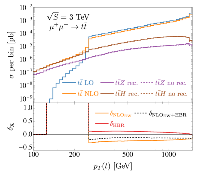
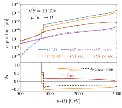
Figure 19: Same as Fig. 18, but imposing the cut $m(t\bar{t})>0.5\sqrt{S}$, unlike as done in general, Eq. (3.1), for the other plots in this work.

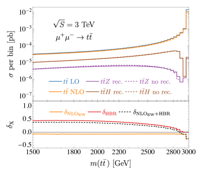
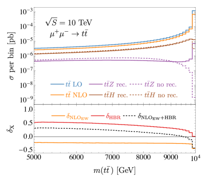
Figure 20: Same as Fig. 19, for the $m(t{\bar{t}})$ distribution in $\mu^{+}\mu^{-}\to t{\bar{t}}$.

We start considering again the $p_{T}(t)$ distribution in $t\bar{t}$ production in Fig. 18. In the main panel we show as in the previous sections LO and $\rm NLO_{EW}$ predictions, but also the contribution to the same observable from the $t\bar{t}Z$ (violet) and $t\bar{t}H$ (brown) production processes. In the solid (dashed) lines correspond to the case “Recombination” (“No recombination”) described in Sec. 3.1. In the first inset we show, as usual, $\delta_{\rm NLO_{EW}}$ as an orange line but also $\delta_{\rm HBR}$ (see Eq. (3.11)) as a red line and $\delta_{\rm NLO_{EW}+HBR}$ (see Eq. (3.13)) as a black dashed line. It is clear that the HBR contribution is given by the sum of $t\bar{t}Z$ and $t\bar{t}H$ and for the sake of simplicity and the purpose of our discussion in the inset we consider only the case where the HBR is recombined with the top quarks.

A couple of features are manifest in Fig. 18. First, the contribution of $t\bar{t}Z$ is much larger than the one from $t\bar{t}H$, so $\delta_{\rm HBR}$ is dominated by the former. Second, we see that at very large $p_{T}(t)$, if top-quarks are recombined with the $B=H,V$ the contribution from both $t\bar{t}H$ and $t\bar{t}Z$ is much larger (solid vs. dashed). Indeed, only via the recombination of a top with the HBR the $t\bar{t}$ pair can reach the value $m(t\bar{t})\simeq s\simeq S$, which would not be possible otherwise even with soft HBR since $M_{B}\neq 0$. We will come back with more details on this point later in the discussion. Third, even considering such a recombination procedure, the total HBR contribution is negligible w.r.t. the effects of the same perturbative order induced by NLO EW corrections, both at 3 and 10 TeV. This can be seen by comparing the absolute values of $\delta_{\rm HBR}$ and $\delta_{\rm NLO_{EW}}$ over the spectrum for $p_{T}(t)\gtrsim 250~{}\,\textrm{GeV}$ ($p_{T}(t)\gtrsim 800~{}\,\textrm{GeV}$) at 3 TeV (10 TeV) collisions. Only for smaller values of $p_{T}(t)$ the HBR contribution is very large, similar to the case of the $\rm NLO_{EW}$ predictions. The same argument presented for explaining the large contribution from the real photon radiation and in turn the $\rm NLO_{EW}$ prediction in the discussion of Fig. 1 can be repeated here for the HBR. Finally, we see that, as a consequence of the previous point, $\delta_{\rm NLO_{EW}}\simeq\delta_{\rm NLO_{EW}+HBR}$ for $p_{T}(t)\gtrsim 250~{}\,\textrm{GeV}$ ($p_{T}(t)\gtrsim 800~{}\,\textrm{GeV}$) at 3 TeV (10 TeV) collisions. This implies the EWSL from weak virtual corrections, i.e. the $\delta_{{\rm SDK_{weak}}}$ prediction which we have been shown to be the dominant component of $\delta_{\rm NLO_{EW}}$ in the discussion of Fig 1, are minimally compensated by those from real radiation.

Let us see how it is possible that the contribution from HBR is much smaller than the one from $\rm NLO_{EW}$, although $\sqrt{S}\gg M_{W}$. First of all, in order to select the direct-production mechanism and exclude VBF configuration, the cut in (3.1) is present in our simulations. Moreover, also the cuts in $\eqref{eq:cuts}$ are present and have to be satisfied. Thus, the phase space of the $H$ and $Z$ radiation is much more constrained than one could naively expect. As a consequence, the double logarithms of the form $L(S,M^{2}_{B})$, as those appearing in the virtual contributions, cannot be present. A larger contribution can be observed if the cut in Eq. (3.1) is relaxed to $m(t\bar{t})\geq 0.5\,\sqrt{S}$, as shown in Fig. 19. However, the effects from HBR are far from being of ${\cal O}(1)$ and are especially much smaller than NLO EW corrections.

While the EWSL from virtual corrections receive contributions from $W$ and $Z$ bosons, at ${\cal O}(\alpha)$ the HBR receive contributions only from the $Z$ boson (and the $H$ boson) emissions and especially are suppressed due to the phase-space cuts. One cannot simply estimate the HBR rescaling the LO predictions by the EWSL as done in the case of virtual contributions. Moreover, as pointed out in Ref. Bagdatova:2024aem , the fact that the $W,Z$, and $H$ have a non-zero mass cannot be neglected and has an impact also in the results that are obtained.

In order to better understand the difference between the case of $\rm NLO_{EW}$ predictions and the HBR, in Fig. 20 we show the $m(t\bar{t})$ distribution in the range $m(t\bar{t})\geq 0.5\,\sqrt{S}$. For such distribution we clearly observe a much larger impact of the HBR w.r.t. the $p_{T}(t)$ case. However, one should, first of all, keep in mind that due to the shape of lepton PDFs, as already said, the direct production mechanism is dominated by $s\simeq S$ and therefore all the $p_{T}(t)$ distribution is mostly correlated to the last bin $m(t\bar{t})\simeq\sqrt{S}$, where instead the HBR contribution is minimal or even zero in the case of no recombination of the top quarks with $B=H,Z$. Thus, there is no contradiction between what is observed in the $m(t\bar{t})$ and $p_{T}(t)$ distributions. First, we explain in more detail the case without recombination and then we move to the case where top quarks are recombined with the HBR.

When $m(t\bar{t})<\sqrt{S}$, at LO it implies $s<S$, and therefore the prediction originates from Bjorken-$x<1$ in the muon PDFs, featuring a very large suppression. Conversely, at $\rm NLO_{EW}$ accuracy, due to the real photon emissions, or thanks to the HBR contributions, if $m(t\bar{t})<\sqrt{S}$ it is still possible to have $\sqrt{s}\simeq\sqrt{S}$ due to the $2\to 3$ kinematic and avoid the suppression of the PDFs. Thus the large relative contribution from HBR ($\delta_{\rm HBR}$) at $m(t\bar{t})\ll\sqrt{S}$ is due in part to the larger phase space volumes for the radiation, as also observed by the comparison of Figs. 18 and 19, but especially to the lack of PDF suppression that is instead present at LO. For $m(t\bar{t})\simeq\sqrt{S}$ it is the opposite; there is no HBR contribution without performing the recombination. Indeed, due to momentum conservation, the relation $m(t\bar{t})<\sqrt{S}-M_{B}$ has to be satisfied.

If the recombination of top quarks with $B=H,Z$ is performed, the predictions at $m(t\bar{t})<\sqrt{S}$ are very similar to the case without recombination. The prediction at $m(t\bar{t})\simeq\sqrt{S}$, especially for the case of the $H$ boson emission, is instead very different. This is not a surprise since when a top is recombined with a $B$ the requirement $m(t\bar{t})\simeq\sqrt{S}$ translates into $m(t\bar{t}B)\simeq\sqrt{S}$ and so the relation $m(t\bar{t})<\sqrt{S}-M_{B}$ has not to be satisfied. We stress again that $\delta_{\rm HBR}$ in the inset corresponds to the case with recombination. The case without it therefore would exhibit even smaller predictions for it.

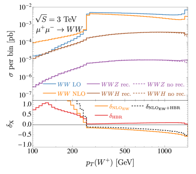
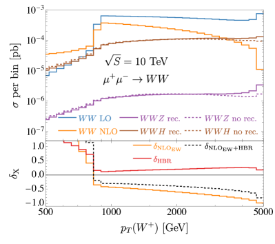
Figure 21: Same as Fig. 19, but for the $p_{T}(W^{+})$ distribution in $\mu^{+}\mu^{-}\to W^{+}W^{-}$. Also in this case $m(t\bar{t})>0.5\sqrt{S}$.

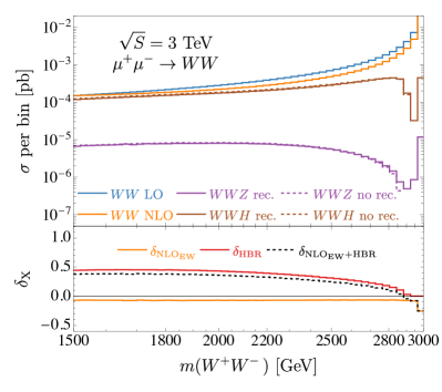
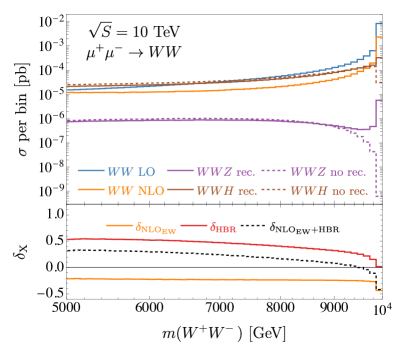
Figure 22: Same as Fig. 21 for the $m(W^{+}W^{-})$ distribution in $\mu^{+}\mu^{-}\to W^{+}W^{-}$.

The dynamics observed for the HBR in $t\bar{t}$ production is not peculiar for this process and we show as a further example the case of $WW$ production. In Fig. 21 we show the $p_{T}(W^{+})$ distribution and in Fig. 22 the $m(W^{+}W^{-})$ distribution, both of them obtained with the cut (3.1) replaced by $m(W^{+}W^{-})>0.5\sqrt{S}$. The $WW$ process is very different from the $t\bar{t}$ one. At LO a $t$-channel diagram is present and the $p_{T}(W^{+})$ distribution is much flatter than the $p_{T}(t)$ in $t\bar{t}$ production. Nevertheless, the same effects observed for $t\bar{t}$ production are present also for this process.

In conclusion, the HBR is not expected in general to lead to large effects in the bulk of the cross sections of direct production processes. Conversely, it can be relevant for instance in regions of the phase space where the cross section is very suppressed at LO, as in the case shown here for $m(F)<\sqrt{S}$. However, as already mentioned before in this paper, further effects have to be considered in these cases, such as effects from other PDFs (photon PDF in the muon). The results of this section show also that while the resummation of EWSL from virtual corrections can be essential, as discussed in Sec. 4.2, in the case of HBR the multiple emission of weak bosons is not expected to be always of primary relevance. That said, we are not claiming that HBR is always leading to a small effect. An example is what is discussed in Ref. Buttazzo:2020uzc , where the $WWH$ production process has been shown to be of the same order as $ZH$ one. In some sense, the $WWH$ can be considered as one of the HBR corrections to $ZH$ production, if the physical object rather than a $Z$ boson is a generic $V$ bosons $V=W,Z$; thus we compare $VH$ and $VVH$ in this case. However, the origin of the large contribution from $WWH$ is not only due to the presence of the double logarithms. Since $ZH$ is an $s-$channel process and in $WWH$ there are instead $t$-channel configurations, featuring less suppression at high-energy, a further enhancement not related to EWSL is present for the HBR w.r.t. the LO prediction. This mechanism is not present in the case of $t\bar{t}$ and $W^{+}W^{-}$ production processes. Rather than a common feature it should be regarded as a special case, similarly to, e.g., the giant QCD $K$-factors observed for some hadroproduction processes Frixione:1992pj ; Frixione:1993yp ; Rubin:2010xp ; Maltoni:2015ena .

4.3.2 EW jets in multi-$V$ production

We now consider the case of inclusive EW-dijet production, $\mu^{+}\mu^{-}\to 2j_{\rm EW}$, where in the EW-jet $j_{\rm EW}$ we cluster $W$ and $Z$ bosons. In other words, the LO originates from the processes $\mu^{+}\mu^{-}\to VV$ with $V=W,Z$, which correspond to the final states $WW$ and $ZZ$. Having found in the previous section that the impact of the Higgs boson radiation is minimal, we consider as a contribution to the HBR only the processes involving an additional $V=W,Z$ radiation, $\mu^{+}\mu^{-}\to 3V$, which correspond to the final states $ZZZ$ and $WWZ$. Clearly, the (at least) two $j_{\rm EW}$’s that are required may be also associated with $W$ and $Z$, respectively, or also with a $WZ$ pair and a $Z$ respectively. Several combinations are possible and some of them, as the ones just mentioned and unlike the cases discussed in the previous section, do not feature the same “partonic” final state of the LO, which can feature only $ZZ$ and $WW$. We will consider also the case of a double HBR and therefore the $4V$ final states: $ZZZZ$, $WWWW$ and $WWZZ$.

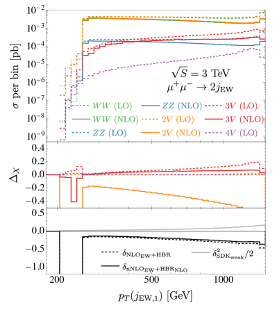
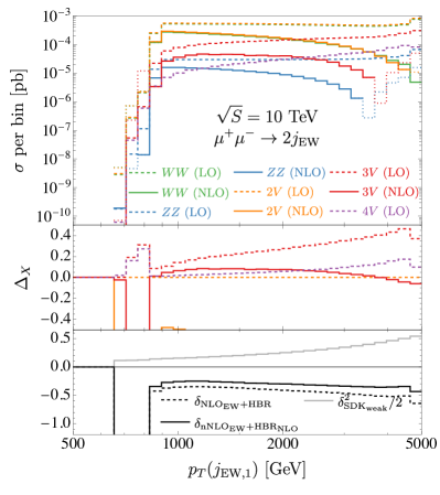
Figure 23: The $p_{T}(j_{{\rm EW},1})$ distribution in $\mu^{+}\mu^{-}\to 2j_{\rm EW}$. The left (right) plot shows results at $\sqrt{S}=3$ TeV ($\sqrt{S}=10$ TeV). The histograms show LO (dashed) and NLO (solid predictions) for $W^{+}W^{-}$ (green), $ZZ$ (blue), $2V=W^{+}W^{-}+ZZ$ (orange), $3V$ (red), and $4V$ (violet, only at the LO). In the second inset, the quantities $\delta_{\rm nNLO_{EW}+HBR_{\rm NLO}}$ and $\delta_{\rm NLO_{EW}+HBR}$ are shown respectively as black-solid and black-dashed lines. These quantities are defined by Eq. (3.26) in terms of respectively Eq. (3.25) and Eq. (3.24). The solid grey line shows the quantity $\delta_{{\rm SDK_{weak}}}^{2}/2$, which enters only in $\delta_{\rm nNLO_{EW}+HBR_{\rm NLO}}$.

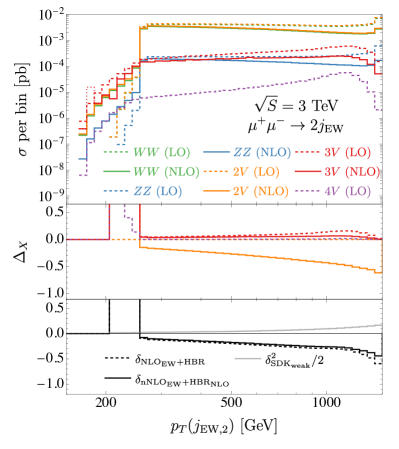
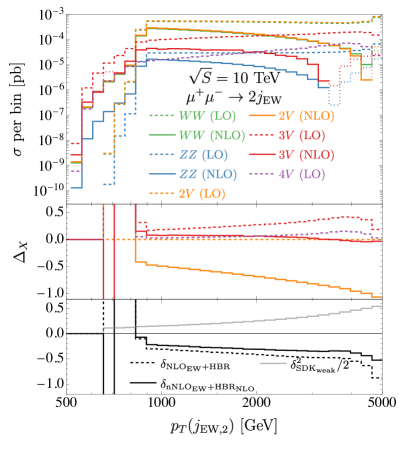
Figure 24: Same as Fig. 23 for the $p_{T}(j_{{\rm EW},2})$ distribution for $\mu^{+}\mu^{-}\to 2j_{\rm EW}$, with $m(2j_{\rm EW})>0.8\sqrt{S}$.

In the plot in Fig. 23 we show the transverse momentum distribution of the hardest $j_{\rm EW}$, $p_{T}(j_{\rm EW,1})$, while in Fig. 24 the same distribution for the second-hardest $j_{\rm EW}$, $p_{T}(j_{\rm EW,2})$. The plots have a different colour code with respect to those shown in the previous sections and we describe them in the following. In the main panel we show the contribution from the $WW$ final state (green) and ZZ (blue) which once summed leads to the $2V$ prediction (orange). The total $3V$ contribution is in red and the $4V$ one in violet. All LO contributions are shown as dashed lines while those at $\rm NLO_{EW}$ accuracy as solid lines.

In the first inset we plot the quantities

$$\Delta_{X}(2V) \equiv \frac{\sigma_{X}(2V)-\sigma_{\rm LO}(2V)}{\sigma_{\rm LO}(2V)}\,.$$ (4.2)

$$\Delta_{X}(3V) \equiv \frac{\sigma_{X}(3V)}{\sigma_{\rm LO}(2V)}$$ (4.3)

$$\Delta_{X}(4V) \equiv \frac{\sigma_{X}(4V)}{\sigma_{\rm LO}(2V)}$$ (4.4)

where $\sigma_{\rm LO}(2V)$ corresponds to the LO predictions for $2j_{\rm EW}$ production. Similarly, $\sigma_{\rm NLO_{EW}}(2V)$ corresponds to the $\rm NLO_{EW}$ prediction for $2j_{\rm EW}$ production, and $\sigma_{\rm LO}(3V)$ to the HBR contribution. Thus, $\Delta_{\rm NLO_{EW}}(2V)=\delta_{\rm NLO_{EW}}(2j_{\rm EW})$ and $\Delta_{{\rm LO}}(3V)=\delta_{\rm HBR}(2j_{\rm EW})$. In the second inset we instead plot the quantities defined in Eqs. (3.24) and (3.25), respectively, as $\delta_{\rm NLO_{EW}+HBR}$ and $\delta_{\rm nNLO_{EW}+HBR_{\rm NLO}}$. The former (the black-dashed line) accounts for all the possible corrections of ${\cal O}(\alpha)$, which are calculated exactly. The latter (the black-solid line) accounts for the former effects plus all the ${\cal O}(\alpha^{2})$ corrections: the double HBR and NLO EW corrections to single HBR, which are evaluated exactly, and the NNLO EW corrections, which are approximated via the EWSL. In particular the contribution from the approximated NNLO EW corrections, i.e., the quantity $\delta_{{\rm SDK_{weak}}}^{2}/{2}$ in Eq. (3.25), is displayed as a grey solid line in the second inset.

In the main panel we notice that the LO is dominated by the $WW$ “partonic” process, which has a much larger cross section than the $ZZ$ “partonic” process and therefore coincides with $2V$. Especially at 10 TeV, both $2V$ and $3V$ processes receive very large and negative contributions from NLO EW corrections. The coloured dotted lines in the main inset of the right plot of Fig. 23 indicates negative values for the lines depicted as solid, which we plot in absolute value in order to be visible on a logarithmic scale. It means that for both $2V$ and $3V$ processes, the relative NLO EW corrections are negative and larger than $100\%$ in absolute value. At 3 TeV they are smaller, but also in this case they are much larger than the contribution from double HBR production at LO, i.e. $4V$ at LO. Similarly to the case of the HBR, i.e. $3V$ at LO, which is smaller than the NLO EW corrections, the double HBR, i.e. $4V$ at LO, is smaller than the NLO EW corrections to $3V$ and so to the single HBR. Estimating the two-loop corrections, i.e. the NNLO to $2V$, as $\delta_{\rm NLO_{EW}}^{2}/2\simeq\delta_{{\rm SDK_{weak}}}^{2}/2$, we see that this contribution (the grey solid line) is even larger than the NLO EW corrections to the HBR contribution. In other words, looking at the case ${\cal O}(\alpha)$ and ${\cal O}(\alpha^{2})$, it appears that for a given $n$ the leading component of the ${\cal O}(\alpha^{n})$ corrections to LO in $2j_{\rm EW}$ production is the $n$-loop corrections, the subleading component is the $(n-1)$-loop corrections to HBR and so on; loops win over HBR.

In the second inset, we see the relative corrections induced by all ${\cal O}(\alpha)$ contributions, $\delta_{\rm NLO_{EW}+HBR}$, are negative and larger in absolute value than the $\delta_{\rm nNLO_{EW}+HBR_{\rm NLO}}$ quantity, which is also negative and includes also the ${\cal O}(\alpha^{2})$ contributions. The NLO EW corrections to HBR are negative but they are completely compensated by the positive $\delta_{{\rm SDK_{weak}}}^{2}/2$ contribution (see Eq. (3.25)) and in part by the double HBR. Without taking into account such contribution, we would see a different picture: $\delta_{\rm nNLO_{EW}+HBR_{\rm NLO}}$ would be much larger than $\delta_{\rm NLO_{EW}+HBR}$ in absolute value. It is also interesting to note how close $\delta_{\rm NLO_{EW}+HBR}$ and $\delta_{\rm nNLO_{EW}+HBR_{\rm NLO}}$ are over the full spectrum.

Unlike what has been done in Sec. 4.2, here we did not approximate via exponentiation the resummation of higher-order EWSL; we have only retained those of ${\cal O}(\alpha^{2})$ arising from such exponentiation in order to approximate the NNLO EW. However, a proper resummation of such effects is also in this case clearly necessary for reliable results at 10 TeV collisions.

We have also inspected the same results allowing $m(j_{\rm EW,1}j_{\rm EW,2})>0.5\sqrt{S}$. Contributions from HBR are slightly more relevant, similarly to what was observed in Sec. 4.3.1, but otherwise the qualitative picture is not altered. Given the results shown in Ref. Buttazzo:2020uzc a different picture may arise if instead of the $2j_{\rm EW}$ processes the $Hj_{\rm EW}$ is considered. We reckon this would be very interesting, but it would not be representative of the typical impact of HBR at muon colliders.

5 Conclusions and outlook

We have performed a comprehensive study of EW corrections at a future multi-TeV muon collider, using the MadGraph5_aMC@NLO framework. The focus of our work has been on direct-production processes. For these colliders, EW corrections are sizeable, and their inclusion is mandatory not just for precision studies, but even for proper estimates of scattering rates. Within MG5_aMC, EW corrections can be computed either exactly, or in the Sudakov (high-energy) approximation, exploiting the DP algorithm. The latter case has clear advantages in terms of speed and numerical stability, however its accuracy must always be validated against the exact NLO EW computation. Indeed, in this respect, we have shown the benefit of employing a purely-weak version of the DP approach, and the importance of including extra angular-dependent terms. Both aspects were first highlighted in Ref. Pagani:2021vyk . Still, we have discussed exceptional cases when the high-energy approximation as obtained from the DP method fails, sometimes in a rather spectacular way, as in the case of $ZHH$ production.

Besides, we have discussed when, due to their large size, the resummation of EW corrections is necessary to have reliable estimates of rates. Although based on an approximate formula, our findings show that resummation is mandatory for very high collider energies or for multi-boson processes or, in general whenever EW corrections easily exceed -50% with respect to the LO rate. In other cases, resummation is still beneficial for precision studies.

Finally, we have discussed the impact of the real-emission counterpart of the Sudakov logarithms, i.e., the radiation of a heavy boson. Generally, the impact of these processes is subdominant w.r.t. their virtual counterpart. This is somehow in disagreement with existing studies on the subject which, however, have focused on specific processes. Indeed, enhancements due to the HBR can be found only for particular processes or regions of the phase space, either when the HBR processes are kinematically favourable w.r.t. the LO (e.g. appearance of $t$ channels), or because the emission of an extra particle modifies phase-space boundaries.

While the study has been carried out focusing on SM processes, many of the conclusions can be considered generic and can be extended to BSM scenarios. Studies aimed at specific extensions of the SM are envisaged.

A natural follow-up of this work is the study of the low-invariant mass region, where direct production is not the dominant mechanism. In this region, photon-initiated processes and VBF topologies are relevant, and a number of aspects need to be under control in order to have reliable predictions. For example, small-$x$ effects in the parton distributions, and the interplay between power corrections and logarithmic enhancements related to the vector-boson mass.

Acknowledgments

Computational resources have been provided by the supercomputing facilities of the Université catholique de Louvain (CISM/UCL) and the Consortium des Équipements de Calcul Intensif en Fédération Wallonie Bruxelles (CÉCI) funded by the Fond de la Recherche Scientifique de Belgique (F.R.S.-FNRS) under convention 2.5020.11 and by the Walloon Region. DP acknowledges support from the DESY computing infrastructures provided through the DESY theory group for the initial stages of this work. The work of M.Z. has been partly supported by the “Programma per Giovani Ricercatori Rita Levi Montalcini” granted by the Italian Ministero dell’Università e della Ricerca (MUR). We also acknowledge support from the COMETA COST Action CA22130.

Appendix A ISR parton distribution

In this Appendix we discuss the modelling of ISR effects and therefore of the muon PDF in our simulations. As it should be clear from the discussion in Sec. 3.1 our interest is in the direct-production processes, characterised by an invariant mass of the produced final state close to the nominal collider energy, $\sqrt{s}\simeq\sqrt{S}$. In this region, the dominant parton luminosity is the muonic one, while all other ones (photon, the other fermions, etc.) are suppressed by large factors. This can be clearly seen, e.g., in several plots that have been shown in Refs. Han:2020uid ; Han:2021kes .

Having established that the only relevant parton is the muon, the next question to address is how to model its luminosity density. At the moment, at variance with the electron case, only LL-accurate muon densities are available. Furthermore, given the results presented in Ref. Bertone:2022ktl for the case of $e^{+}e^{-}$ collisions, one can appreciate that the size of effects on physical observables, due to the NLL evolution or the various factorisation schemes at this order, is at the percent level or below. EW corrections instead, as documented also in Sec. 4, lie in the ball-park of several tens of percent for direct production processes at a high-energy muon collider. Moreover, the modelling of ISR, although being of primary relevance for precision studies, is not one of the several aspects (see Sec. 3.3) that we are investigating in this work.

Given all the previous considerations, a LL description for the muon PDF is sufficient for our simulations. We reckon that, quite recently, a fully-fledged description of the muonic content in terms of massless partons (leptons, the photon, but also quarks and the gluon) has appeared in Ref. Frixione:2023gmf , employing LL-accurate evolution in QCD and QED. For the purpose of this work, however, we opt for a simpler approach. Specifically, we minimally modify the electron ISR PDF at Leading-Logarithmic (LL) accuracy Gribov:1972ri ; Lipatov:1974qm ; Altarelli:1977zs ; Dokshitzer:1977sg in the so-called $\beta$ scheme, including up to $\mathcal{O}(\alpha^{3})$ terms Skrzypek:1990qs ; Skrzypek:1992vk ; Cacciari:1992pz :

$$\Gamma^{\rm LL}_{\mu^{\pm}/\mu^{\pm}}(x,Q^{2})=\frac{\exp(-\gamma_{E}\beta+\frac{3}{4}\beta)}{\Gamma(1+\beta)}\beta(1-x)^{\beta-1}-\sum_{n=1}^{3}\frac{1}{2^{n}n!}\beta^{n}h_{n}(x)\,,$$ (A.1)

where

$$\beta=\frac{\alpha}{\pi}\left(\log(Q^{2}/m^{2})-1\right)\,.$$ (A.2)

We then set $m$ to the muon mass, and we neglect the running of $\alpha$. Rather, we fix its value to

$$\alpha=\alpha_{G_{\mu}}\equiv\frac{G_{\mu}}{\pi}\sqrt{2}\left(1-\frac{M_{W}^{2}}{M_{Z}^{2}}\right)M_{W}^{2}\,,$$ (A.3)

consistently with the renormalisation scheme that we will employ in the computations, with $G_{\mu}$ measured from the muon decay. Finally, as it is well known, the usage of LL-accurate ISR in NLO EW computations requires the inclusion, at the level of short-distance cross section, of additional terms required to attain formal NLO accuracy (treated on the same footage as change of factorisation-scheme contributions) . All our results at NLO will be computed including these terms, which are already available inside MadGraph5_aMC@NLO.

References

- (1) Muon Collider collaboration, The physics case of a 3 TeV muon collider stage, 2203.07261.
- (2) C. Aime et al., Muon Collider Physics Summary, 2203.07256.
- (3) K.M. Black et al., Muon Collider Forum report, JINST 19 (2024) T02015 [2209.01318].
- (4) F. Maltoni et al., TF07 Snowmass Report: Theory of Collider Phenomena, 2210.02591.
- (5) A. Belloni et al., Report of the Topical Group on Electroweak Precision Physics and Constraining New Physics for Snowmass 2021, 2209.08078.
- (6) C. Accettura et al., Towards a muon collider, Eur. Phys. J. C 83 (2023) 864 [2303.08533].
- (7) J.P. Delahaye, M. Diemoz, K. Long, B. Mansoulié, N. Pastrone, L. Rivkin et al., Muon Colliders, 1901.06150.
- (8) N. Bartosik et al., Detector and Physics Performance at a Muon Collider, JINST 15 (2020) P05001 [2001.04431].
- (9) D. Schulte, J.-P. Delahaye, M. Diemoz, K. Long, B. Mansoulié, N. Pastrone et al., Prospects on Muon Colliders, PoS ICHEP2020 (2021) 703.
- (10) K. Long, D. Lucchesi, M. Palmer, N. Pastrone, D. Schulte and V. Shiltsev, Muon colliders to expand frontiers of particle physics, Nature Phys. 17 (2021) 289 [2007.15684].
- (11) Muon Collider collaboration, A Muon Collider Facility for Physics Discovery, 2203.08033.
- (12) Muon Collider collaboration, Simulated Detector Performance at the Muon Collider, 2203.07964.
- (13) Muon Collider collaboration, Promising Technologies and R&D Directions for the Future Muon Collider Detectors, 2203.07224.
- (14) T. Han, D. Liu, I. Low and X. Wang, Electroweak couplings of the Higgs boson at a multi-TeV muon collider, Phys. Rev. D 103 (2021) 013002 [2008.12204].
- (15) D. Buttazzo, R. Franceschini and A. Wulzer, Two Paths Towards Precision at a Very High Energy Lepton Collider, JHEP 05 (2021) 219 [2012.11555].
- (16) T. Han, W. Kilian, N. Kreher, Y. Ma, J. Reuter, T. Striegl et al., Precision test of the muon-Higgs coupling at a high-energy muon collider, JHEP 12 (2021) 162 [2108.05362].
- (17) J. Reuter, T. Han, W. Kilian, N. Kreher, Y. Ma, T. Striegl et al., Precision test of the muon-Higgs coupling at a high-energy muon collider, PoS ICHEP2022 (2022) 1239 [2212.01323].
- (18) E. Celada, T. Han, W. Kilian, N. Kreher, Y. Ma, F. Maltoni et al., Probing Higgs-muon interactions at a multi-TeV muon collider, JHEP 08 (2024) 021 [2312.13082].
- (19) M. Forslund and P. Meade, High precision higgs from high energy muon colliders, JHEP 08 (2022) 185 [2203.09425].
- (20) M. Chen and D. Liu, Top Yukawa coupling measurement at the muon collider, Phys. Rev. D 109 (2024) 075020 [2212.11067].
- (21) M. Ruhdorfer, E. Salvioni and A. Wulzer, Invisible Higgs boson decay from forward muons at a muon collider, Phys. Rev. D 107 (2023) 095038 [2303.14202].
- (22) T. Han, D. Liu, I. Low and X. Wang, Electroweak scattering at the muon shot, Phys. Rev. D 110 (2024) 013005 [2312.07670].
- (23) R. Dermisek, K. Hermanek, T. Lee, N. McGinnis and S. Yoon, Multi-Higgs boson signals of a modified muon Yukawa coupling at a muon collider, Phys. Rev. D 109 (2024) 095003 [2311.05078].
- (24) Z. Liu, K.-F. Lyu, I. Mahbub and L.-T. Wang, Top Yukawa coupling determination at high energy muon collider, Phys. Rev. D 109 (2024) 035021 [2308.06323].
- (25) P. Li, Z. Liu and K.-F. Lyu, Higgs boson width and couplings at high energy muon colliders with forward muon detection, Phys. Rev. D 109 (2024) 073009 [2401.08756].
- (26) T. Han, S. Li, S. Su, W. Su and Y. Wu, BSM Higgs Production at a Muon Collider, in Snowmass 2021, 5, 2022 [2205.11730].
- (27) P. Bandyopadhyay and A. Costantini, Obscure Higgs boson at Colliders, Phys. Rev. D 103 (2021) 015025 [2010.02597].
- (28) T. Han, S. Li, S. Su, W. Su and Y. Wu, Heavy Higgs bosons in 2HDM at a muon collider, Phys. Rev. D 104 (2021) 055029 [2102.08386].
- (29) P. Bandyopadhyay, S. Parashar, C. Sen and J. Song, Probing Inert Triplet Model at a multi-TeV muon collider via vector boson fusion with forward muon tagging, JHEP 07 (2024) 253 [2401.02697].
- (30) B.A. Ouazghour, A. Arhrib, K. Cheung, E.-s. Ghourmin and L. Rahili, Comparison between -+ and e-e+ colliders for charged Higgs production in the 2HDM, Phys. Rev. D 109 (2024) 115009 [2308.15664].
- (31) A. Jueid, T.A. Chowdhury, S. Nasri and S. Saad, Probing Zee-Babu states at muon colliders, Phys. Rev. D 109 (2024) 075011 [2306.01255].
- (32) T. Han, Z. Liu, L.-T. Wang and X. Wang, WIMPs at High Energy Muon Colliders, Phys. Rev. D 103 (2021) 075004 [2009.11287].
- (33) R. Capdevilla, F. Meloni, R. Simoniello and J. Zurita, Hunting wino and higgsino dark matter at the muon collider with disappearing tracks, JHEP 06 (2021) 133 [2102.11292].
- (34) T. Han, Z. Liu, L.-T. Wang and X. Wang, WIMP Dark Matter at High Energy Muon Colliders A White Paper for Snowmass 2021, in Snowmass 2021, 3, 2022 [2203.07351].
- (35) C. Cesarotti and G. Krnjaic, Hitting the Thermal Target for Leptophilic Dark Matter, 2404.02906.
- (36) P. Asadi, A. Radick and T.-T. Yu, Interplay of freeze-in and freeze-out: Lepton-flavored dark matter and muon colliders, Phys. Rev. D 110 (2024) 035022 [2312.03826].
- (37) M. Belfkir, A. Jueid and S. Nasri, Boosting dark matter searches at muon colliders with machine learning: The mono-Higgs channel as a case study, PTEP 2023 (2023) 123B03 [2309.11241].
- (38) A. Jueid and S. Nasri, Lepton portal dark matter at muon colliders: Total rates and generic features for phenomenologically viable scenarios, Phys. Rev. D 107 (2023) 115027 [2301.12524].
- (39) G.-y. Huang, F.S. Queiroz and W. Rodejohann, Gauged at a muon collider, Phys. Rev. D 103 (2021) 095005 [2101.04956].
- (40) G.-y. Huang, S. Jana, F.S. Queiroz and W. Rodejohann, Probing the RK(*) anomaly at a muon collider, Phys. Rev. D 105 (2022) 015013 [2103.01617].
- (41) R.-Y. He, J.-Q. Huang, J.-Y. Xu, F.-X. Yang, Z.-L. Han and F.-L. Shao, Heavy neutral leptons in gauged at muon collider, Chin. Phys. C 48 (2024) 093102 [2401.14687].
- (42) D. Buttazzo and P. Paradisi, Probing the muon anomaly with the Higgs boson at a muon collider, Phys. Rev. D 104 (2021) 075021 [2012.02769].
- (43) R. Capdevilla, D. Curtin, Y. Kahn and G. Krnjaic, Discovering the physics of at future muon colliders, Phys. Rev. D 103 (2021) 075028 [2006.16277].
- (44) W. Yin and M. Yamaguchi, Muon g-2 at a multi-TeV muon collider, Phys. Rev. D 106 (2022) 033007 [2012.03928].
- (45) R. Capdevilla, D. Curtin, Y. Kahn and G. Krnjaic, No-lose theorem for discovering the new physics of at muon colliders, Phys. Rev. D 105 (2022) 015028 [2101.10334].
- (46) J. Gu, L.-T. Wang and C. Zhang, Unambiguously Testing Positivity at Lepton Colliders, Phys. Rev. Lett. 129 (2022) 011805 [2011.03055].
- (47) A. Costantini, F. De Lillo, F. Maltoni, L. Mantani, O. Mattelaer, R. Ruiz et al., Vector boson fusion at multi-TeV muon colliders, JHEP 09 (2020) 080 [2005.10289].
- (48) P. Bandyopadhyay, A. Karan, R. Mandal and S. Parashar, Distinguishing signatures of scalar leptoquarks at hadron and muon colliders, Eur. Phys. J. C 82 (2022) 916 [2108.06506].
- (49) S. Qian, C. Li, Q. Li, F. Meng, J. Xiao, T. Yang et al., Searching for heavy leptoquarks at a muon collider, JHEP 12 (2021) 047 [2109.01265].
- (50) Y. Bao, J. Fan and L. Li, Electroweak ALP searches at a muon collider, JHEP 08 (2022) 276 [2203.04328].
- (51) N. Ghosh, S.K. Rai and T. Samui, Search for a leptoquark and vector-like lepton in a muon collider, Nucl. Phys. B 1004 (2024) 116564 [2309.07583].
- (52) R. Dermisek, K. Hermanek, N. McGinnis and S. Yoon, Predictions for muon electric and magnetic dipole moments from h→+- in two-Higgs-doublet models with new leptons, Phys. Rev. D 108 (2023) 055019 [2306.13212].
- (53) W. Altmannshofer, S.A. Gadam and S. Profumo, Probing new physics with +-→bs at a muon collider, Phys. Rev. D 108 (2023) 115033 [2306.15017].
- (54) D. Liu, L.-T. Wang and K.-P. Xie, Composite resonances at a 10 TeV muon collider, JHEP 04 (2024) 084 [2312.09117].
- (55) S. Sun, Q.-S. Yan, X. Zhao and Z. Zhao, Constraining rare B decays by +-→tc at future lepton colliders, Phys. Rev. D 108 (2023) 075016 [2302.01143].
- (56) T.H. Kwok, L. Li, T. Liu and A. Rock, Searching for Heavy Neutral Leptons at A Future Muon Collider, 2301.05177.
- (57) C. Cesarotti and R. Gambhir, The new physics case for beam-dump experiments with accelerated muon beams, JHEP 05 (2024) 283 [2310.16110].
- (58) Y. Ema, Z. Liu, K.-F. Lyu and M. Pospelov, Heavy Neutral Leptons from Stopped Muons and Pions, JHEP 08 (2023) 169 [2306.07315].
- (59) P. Li, Z. Liu and K.-F. Lyu, Heavy neutral leptons at muon colliders, JHEP 03 (2023) 231 [2301.07117].
- (60) FCC collaboration, FCC-ee: The Lepton Collider: Future Circular Collider Conceptual Design Report Volume 2, Eur. Phys. J. ST 228 (2019) 261.
- (61) G. Bernardi et al., The Future Circular Collider: a Summary for the US 2021 Snowmass Process, 2203.06520.
- (62) CEPC Study Group collaboration, CEPC Conceptual Design Report: Volume 1 - Accelerator, 1809.00285.
- (63) CEPC Study Group collaboration, CEPC Conceptual Design Report: Volume 2 - Physics & Detector, 1811.10545.
- (64) F. An et al., Precision Higgs physics at the CEPC, Chin. Phys. C 43 (2019) 043002 [1810.09037].
- (65) CEPC Accelerator Study Group collaboration, CEPC Input to the ESPP 2018 -Accelerator, 1901.03169.
- (66) CEPC Physics Study Group collaboration, The Physics potential of the CEPC. Prepared for the US Snowmass Community Planning Exercise (Snowmass 2021), in Snowmass 2021, 5, 2022 [2205.08553].
- (67) CEPC Study Group collaboration, CEPC Technical Design Report: Accelerator, Radiat. Detect. Technol. Methods 8 (2024) 1 [2312.14363].
- (68) S. Chen, A. Glioti, R. Rattazzi, L. Ricci and A. Wulzer, Learning from radiation at a very high energy lepton collider, JHEP 05 (2022) 180 [2202.10509].
- (69) H. Al Ali et al., The muon Smasher’s guide, Rept. Prog. Phys. 85 (2022) 084201 [2103.14043].
- (70) R. Ruiz, A. Costantini, F. Maltoni and O. Mattelaer, The Effective Vector Boson Approximation in high-energy muon collisions, JHEP 06 (2022) 114 [2111.02442].
- (71) T. Han, Y. Ma and K. Xie, High energy leptonic collisions and electroweak parton distribution functions, Phys. Rev. D 103 (2021) L031301 [2007.14300].
- (72) T. Han, Y. Ma and K. Xie, Quark and gluon contents of a lepton at high energies, JHEP 02 (2022) 154 [2103.09844].
- (73) F. Garosi, D. Marzocca and S. Trifinopoulos, LePDF: Standard Model PDFs for high-energy lepton colliders, JHEP 09 (2023) 107 [2303.16964].
- (74) V.V. Sudakov, Vertex parts at very high-energies in quantum electrodynamics, Sov. Phys. JETP 3 (1956) 65.
- (75) A. Denner and S. Pozzorini, One loop leading logarithms in electroweak radiative corrections. 1. Results, Eur. Phys. J. C 18 (2001) 461 [hep-ph/0010201].
- (76) A. Denner and S. Pozzorini, One loop leading logarithms in electroweak radiative corrections. 2. Factorization of collinear singularities, Eur. Phys. J. C 21 (2001) 63 [hep-ph/0104127].
- (77) A. Denner, M. Melles and S. Pozzorini, Two loop electroweak angular dependent logarithms at high-energies, Nucl. Phys. B 662 (2003) 299 [hep-ph/0301241].
- (78) A. Denner and S. Pozzorini, An Algorithm for the high-energy expansion of multi-loop diagrams to next-to-leading logarithmic accuracy, Nucl. Phys. B 717 (2005) 48 [hep-ph/0408068].
- (79) A. Denner, B. Jantzen and S. Pozzorini, Two-loop electroweak next-to-leading logarithmic corrections to massless fermionic processes, Nucl. Phys. B 761 (2007) 1 [hep-ph/0608326].
- (80) A. Denner, B. Jantzen and S. Pozzorini, Two-loop electroweak next-to-leading logarithms for processes involving heavy quarks, JHEP 11 (2008) 062 [0809.0800].
- (81) E. Bothmann and D. Napoletano, Automated evaluation of electroweak Sudakov logarithms in Sherpa, Eur. Phys. J. C 80 (2020) 1024 [2006.14635].
- (82) Sherpa collaboration, Event Generation with Sherpa 2.2, SciPost Phys. 7 (2019) 034 [1905.09127].
- (83) D. Pagani and M. Zaro, One-loop electroweak Sudakov logarithms: a revisitation and automation, JHEP 02 (2022) 161 [2110.03714].
- (84) J. Alwall, R. Frederix, S. Frixione, V. Hirschi, F. Maltoni, O. Mattelaer et al., The automated computation of tree-level and next-to-leading order differential cross sections, and their matching to parton shower simulations, JHEP 07 (2014) 079 [1405.0301].
- (85) R. Frederix, S. Frixione, V. Hirschi, D. Pagani, H.S. Shao and M. Zaro, The automation of next-to-leading order electroweak calculations, JHEP 07 (2018) 185 [1804.10017].
- (86) D. Pagani, T. Vitos and M. Zaro, Improving NLO QCD event generators with high-energy EW corrections, Eur. Phys. J. C 84 (2024) 514 [2309.00452].
- (87) J.M. Lindert and L. Mai, Logarithmic EW corrections at one-loop, 2312.07927.
- (88) F. Cascioli, P. Maierhofer and S. Pozzorini, Scattering Amplitudes with Open Loops, Phys. Rev. Lett. 108 (2012) 111601 [1111.5206].
- (89) F. Buccioni, J.-N. Lang, J.M. Lindert, P. Maierhöfer, S. Pozzorini, H. Zhang et al., OpenLoops 2, Eur. Phys. J. C 79 (2019) 866 [1907.13071].
- (90) J.-y. Chiu, F. Golf, R. Kelley and A.V. Manohar, Electroweak Sudakov corrections using effective field theory, Phys. Rev. Lett. 100 (2008) 021802 [0709.2377].
- (91) J.-y. Chiu, R. Kelley and A.V. Manohar, Electroweak Corrections using Effective Field Theory: Applications to the LHC, Phys. Rev. D 78 (2008) 073006 [0806.1240].
- (92) A.V. Manohar and W.J. Waalewijn, Electroweak Logarithms in Inclusive Cross Sections, JHEP 08 (2018) 137 [1802.08687].
- (93) C.W. Bauer, S. Fleming and M.E. Luke, Summing Sudakov logarithms in in effective field theory., Phys. Rev. D 63 (2000) 014006 [hep-ph/0005275].
- (94) C.W. Bauer, S. Fleming, D. Pirjol and I.W. Stewart, An Effective field theory for collinear and soft gluons: Heavy to light decays, Phys. Rev. D 63 (2001) 114020 [hep-ph/0011336].
- (95) C.W. Bauer and I.W. Stewart, Invariant operators in collinear effective theory, Phys. Lett. B 516 (2001) 134 [hep-ph/0107001].
- (96) C.W. Bauer, D. Pirjol and I.W. Stewart, Soft collinear factorization in effective field theory, Phys. Rev. D 65 (2002) 054022 [hep-ph/0109045].
- (97) A. Denner and S. Rode, Automated resummation of electroweak Sudakov logarithms in diboson production at future colliders, Eur. Phys. J. C 84 (2024) 542 [2402.10503].
- (98) M. Aicheler, P. Burrows, M. Draper, T. Garvey, P. Lebrun, K. Peach et al., eds., A Multi-TeV Linear Collider Based on CLIC Technology: CLIC Conceptual Design Report, .
- (99) L. Linssen, A. Miyamoto, M. Stanitzki and H. Weerts, eds., Physics and Detectors at CLIC: CLIC Conceptual Design Report, 1202.5940.
- (100) P. Lebrun, L. Linssen, A. Lucaci-Timoce, D. Schulte, F. Simon, S. Stapnes et al., The CLIC Programme: Towards a Staged e+e- Linear Collider Exploring the Terascale : CLIC Conceptual Design Report, 1209.2543.
- (101) CLIC, CLICdp collaboration, Updated baseline for a staged Compact Linear Collider, 1608.07537.
- (102) CLICdp, CLIC collaboration, The Compact Linear Collider (CLIC) - 2018 Summary Report, 1812.06018.
- (103) O. Brunner et al., The CLIC project, 2203.09186.
- (104) FCC collaboration, FCC Physics Opportunities: Future Circular Collider Conceptual Design Report Volume 1, Eur. Phys. J. C 79 (2019) 474.
- (105) FCC collaboration, FCC-hh: The Hadron Collider: Future Circular Collider Conceptual Design Report Volume 3, Eur. Phys. J. ST 228 (2019) 755.
- (106) M. Benedikt et al., Future Circular Hadron Collider FCC-hh: Overview and Status, 2203.07804.
- (107) P. Ciafaloni, D. Comelli, A. Riotto, F. Sala, A. Strumia and A. Urbano, Weak Corrections are Relevant for Dark Matter Indirect Detection, JCAP 03 (2011) 019 [1009.0224].
- (108) S. Kallweit, J.M. Lindert, P. Maierhöfer, S. Pozzorini and M. Schönherr, NLO electroweak automation and precise predictions for W+multijet production at the LHC, JHEP 04 (2015) 012 [1412.5157].
- (109) S. Frixione, V. Hirschi, D. Pagani, H.S. Shao and M. Zaro, Electroweak and QCD corrections to top-pair hadroproduction in association with heavy bosons, JHEP 06 (2015) 184 [1504.03446].
- (110) M. Chiesa, N. Greiner and F. Tramontano, Automation of electroweak corrections for LHC processes, J. Phys. G 43 (2016) 013002 [1507.08579].
- (111) B. Biedermann, S. Bräuer, A. Denner, M. Pellen, S. Schumann and J.M. Thompson, Automation of NLO QCD and EW corrections with Sherpa and Recola, Eur. Phys. J. C 77 (2017) 492 [1704.05783].
- (112) M. Chiesa, N. Greiner, M. Schönherr and F. Tramontano, Electroweak corrections to diphoton plus jets, JHEP 10 (2017) 181 [1706.09022].
- (113) D. Pagani, H.-S. Shao, I. Tsinikos and M. Zaro, Automated EW corrections with isolated photons: t, t and tj as case studies, JHEP 09 (2021) 155 [2106.02059].
- (114) V. Bertone, M. Cacciari, S. Frixione, G. Stagnitto, M. Zaro and X. Zhao, Improving methods and predictions at high-energy e+e- colliders within collinear factorisation, JHEP 10 (2022) 089 [2207.03265].
- (115) P.M. Bredt, W. Kilian, J. Reuter and P. Stienemeier, NLO electroweak corrections to multi-boson processes at a muon collider, JHEP 12 (2022) 138 [2208.09438].
- (116) S. Frixione, V. Hirschi, D. Pagani, H.S. Shao and M. Zaro, Weak corrections to Higgs hadroproduction in association with a top-quark pair, JHEP 09 (2014) 065 [1407.0823].
- (117) D. Pagani, I. Tsinikos and M. Zaro, The impact of the photon PDF and electroweak corrections on distributions, Eur. Phys. J. C 76 (2016) 479 [1606.01915].
- (118) R. Frederix, S. Frixione, V. Hirschi, D. Pagani, H.-S. Shao and M. Zaro, The complete NLO corrections to dijet hadroproduction, JHEP 04 (2017) 076 [1612.06548].
- (119) M. Czakon, D. Heymes, A. Mitov, D. Pagani, I. Tsinikos and M. Zaro, Top-pair production at the LHC through NNLO QCD and NLO EW, JHEP 10 (2017) 186 [1705.04105].
- (120) R. Frederix, D. Pagani and M. Zaro, Large NLO corrections in and hadroproduction from supposedly subleading EW contributions, JHEP 02 (2018) 031 [1711.02116].
- (121) A. Broggio, A. Ferroglia, R. Frederix, D. Pagani, B.D. Pecjak and I. Tsinikos, Top-quark pair hadroproduction in association with a heavy boson at NLO+NNLL including EW corrections, JHEP 08 (2019) 039 [1907.04343].
- (122) R. Frederix, D. Pagani and I. Tsinikos, Precise predictions for single-top production: the impact of EW corrections and QCD shower on the -channel signature, JHEP 09 (2019) 122 [1907.12586].
- (123) D. Pagani, H.-S. Shao and M. Zaro, RIP : how other Higgs production modes conspire to kill a rare signal at the LHC, JHEP 11 (2020) 036 [2005.10277].
- (124) D. Pagani, I. Tsinikos and E. Vryonidou, NLO QCD+EW predictions for and production at the LHC, JHEP 08 (2020) 082 [2006.10086].
- (125) F. Maltoni, D. Pagani and S. Tentori, Top-quark pair production as a probe of light top-philic scalars and anomalous Higgs interactions, 2406.06694.
- (126) H. El Faham, K. Mimasu, D. Pagani, C. Severi, E. Vryonidou and Z. M., In preparation, .
- (127) S. Frixione, Z. Kunszt and A. Signer, Three jet cross-sections to next-to-leading order, Nucl. Phys. B 467 (1996) 399 [hep-ph/9512328].
- (128) S. Frixione, A General approach to jet cross-sections in QCD, Nucl. Phys. B 507 (1997) 295 [hep-ph/9706545].
- (129) R. Frederix, S. Frixione, F. Maltoni and T. Stelzer, Automation of next-to-leading order computations in QCD: The FKS subtraction, JHEP 10 (2009) 003 [0908.4272].
- (130) R. Frederix, S. Frixione, A.S. Papanastasiou, S. Prestel and P. Torrielli, Off-shell single-top production at NLO matched to parton showers, JHEP 06 (2016) 027 [1603.01178].
- (131) G. Ossola, C.G. Papadopoulos and R. Pittau, Reducing full one-loop amplitudes to scalar integrals at the integrand level, Nucl. Phys. B 763 (2007) 147 [hep-ph/0609007].
- (132) G. Passarino and M.J.G. Veltman, One Loop Corrections for e+ e- Annihilation Into mu+ mu- in the Weinberg Model, Nucl. Phys. B 160 (1979) 151.
- (133) A.I. Davydychev, A Simple formula for reducing Feynman diagrams to scalar integrals, Phys. Lett. B 263 (1991) 107.
- (134) A. Denner and S. Dittmaier, Reduction schemes for one-loop tensor integrals, Nucl. Phys. B 734 (2006) 62 [hep-ph/0509141].
- (135) P. Mastrolia, E. Mirabella and T. Peraro, Integrand reduction of one-loop scattering amplitudes through Laurent series expansion, JHEP 06 (2012) 095 [1203.0291].
- (136) G. Ossola, C.G. Papadopoulos and R. Pittau, CutTools: A Program implementing the OPP reduction method to compute one-loop amplitudes, JHEP 03 (2008) 042 [0711.3596].
- (137) H.-S. Shao, IREGI user’s manual, Unpublished .
- (138) T. Peraro, Ninja: Automated Integrand Reduction via Laurent Expansion for One-Loop Amplitudes, Comput. Phys. Commun. 185 (2014) 2771 [1403.1229].
- (139) V. Hirschi and T. Peraro, Tensor integrand reduction via Laurent expansion, JHEP 06 (2016) 060 [1604.01363].
- (140) A. Denner, S. Dittmaier and L. Hofer, COLLIER - A fortran-library for one-loop integrals, PoS LL2014 (2014) 071 [1407.0087].
- (141) A. Denner, S. Dittmaier and L. Hofer, Collier: a fortran-based Complex One-Loop LIbrary in Extended Regularizations, Comput. Phys. Commun. 212 (2017) 220 [1604.06792].
- (142) V. Hirschi, R. Frederix, S. Frixione, M.V. Garzelli, F. Maltoni and R. Pittau, Automation of one-loop QCD corrections, JHEP 05 (2011) 044 [1103.0621].
- (143) S. Frixione and B.R. Webber, Matching NLO QCD computations and parton shower simulations, JHEP 06 (2002) 029 [hep-ph/0204244].
- (144) M. Czakon, D. Heymes, A. Mitov, D. Pagani, I. Tsinikos and M. Zaro, Top-quark charge asymmetry at the LHC and Tevatron through NNLO QCD and NLO EW, Phys. Rev. D 98 (2018) 014003 [1711.03945].
- (145) R. Frederix and I. Tsinikos, On improving NLO merging for production, JHEP 11 (2021) 029 [2108.07826].
- (146) R. Frederix, I. Tsinikos and T. Vitos, Probing the spin correlations of production at NLO QCD+EW, Eur. Phys. J. C 81 (2021) 817 [2105.11478].
- (147) S. Frixione, Initial conditions for electron and photon structure and fragmentation functions, JHEP 11 (2019) 158 [1909.03886].
- (148) V. Bertone, M. Cacciari, S. Frixione and G. Stagnitto, The partonic structure of the electron at the next-to-leading logarithmic accuracy in QED, JHEP 03 (2020) 135 [1911.12040].
- (149) S. Frixione, On factorisation schemes for the electron parton distribution functions in QED, JHEP 07 (2021) 180 [2105.06688].
- (150) S. Frixione, O. Mattelaer, M. Zaro and X. Zhao, Lepton collisions in MadGraph5_aMC@NLO, 2108.10261.
- (151) D. Buarque Franzosi et al., Vector boson scattering processes: Status and prospects, Rev. Phys. 8 (2022) 100071 [2106.01393].
- (152) E. Bothmann, D. Napoletano, M. Schönherr, S. Schumann and S.L. Villani, Higher-order EW corrections in ZZ and ZZj production at the LHC, JHEP 06 (2022) 064 [2111.13453].
- (153) S. Dawson, The Effective W Approximation, Nucl. Phys. B 249 (1985) 42.
- (154) G.L. Kane, W.W. Repko and W.B. Rolnick, The Effective W+-, Z0 Approximation for High-Energy Collisions, Phys. Lett. B 148 (1984) 367.
- (155) C.F. von Weizsacker, Radiation emitted in collisions of very fast electrons, Z. Phys. 88 (1934) 612.
- (156) E.J. Williams, Nature of the high-energy particles of penetrating radiation and status of ionization and radiation formulae, Phys. Rev. 45 (1934) 729.
- (157) M. Cacciari, G.P. Salam and G. Soyez, FastJet User Manual, Eur. Phys. J. C 72 (2012) 1896 [1111.6097].
- (158) Y.L. Dokshitzer, G.D. Leder, S. Moretti and B.R. Webber, Better jet clustering algorithms, JHEP 08 (1997) 001 [hep-ph/9707323].
- (159) J.H. Kuhn, A.A. Penin and V.A. Smirnov, Summing up subleading Sudakov logarithms, Eur. Phys. J. C 17 (2000) 97 [hep-ph/9912503].
- (160) V.S. Fadin, L.N. Lipatov, A.D. Martin and M. Melles, Resummation of double logarithms in electroweak high-energy processes, Phys. Rev. D 61 (2000) 094002 [hep-ph/9910338].
- (161) P. Ciafaloni and D. Comelli, Electroweak Sudakov form-factors and nonfactorizable soft QED effects at NLC energies, Phys. Lett. B 476 (2000) 49 [hep-ph/9910278].
- (162) M. Beccaria, F.M. Renard and C. Verzegnassi, Top quark production at future lepton colliders in the asymptotic regime, Phys. Rev. D 63 (2001) 053013 [hep-ph/0010205].
- (163) M. Hori, H. Kawamura and J. Kodaira, Electroweak Sudakov at two loop level, Phys. Lett. B 491 (2000) 275 [hep-ph/0007329].
- (164) M. Ciafaloni, P. Ciafaloni and D. Comelli, Bloch-Nordsieck violating electroweak corrections to inclusive TeV scale hard processes, Phys. Rev. Lett. 84 (2000) 4810 [hep-ph/0001142].
- (165) M. Melles, Electroweak radiative corrections in high-energy processes, Phys. Rept. 375 (2003) 219 [hep-ph/0104232].
- (166) W. Beenakker and A. Werthenbach, Electroweak two loop Sudakov logarithms for on-shell fermions and bosons, Nucl. Phys. B 630 (2002) 3 [hep-ph/0112030].
- (167) S. Pozzorini, Next to leading mass singularities in two loop electroweak singlet form-factors, Nucl. Phys. B 692 (2004) 135 [hep-ph/0401087].
- (168) B. Feucht, J.H. Kuhn, A.A. Penin and V.A. Smirnov, Two loop Sudakov form-factor in a theory with mass gap, Phys. Rev. Lett. 93 (2004) 101802 [hep-ph/0404082].
- (169) B. Jantzen, J.H. Kuhn, A.A. Penin and V.A. Smirnov, Two-loop electroweak logarithms, Phys. Rev. D 72 (2005) 051301 [hep-ph/0504111].
- (170) B. Jantzen, J.H. Kuhn, A.A. Penin and V.A. Smirnov, Two-loop electroweak logarithms in four-fermion processes at high energy, Nucl. Phys. B 731 (2005) 188 [hep-ph/0509157].
- (171) B. Jantzen and V.A. Smirnov, The Two-loop vector form-factor in the Sudakov limit, Eur. Phys. J. C 47 (2006) 671 [hep-ph/0603133].
- (172) A.V. Manohar and M. Trott, Electroweak Sudakov Corrections and the Top Quark Forward-Backward Asymmetry, Phys. Lett. B 711 (2012) 313 [1201.3926].
- (173) C.W. Bauer, N. Ferland and B.R. Webber, Combining initial-state resummation with fixed-order calculations of electroweak corrections, JHEP 04 (2018) 125 [1712.07147].
- (174) M.L. Mangano et al., Physics at a 100 TeV pp Collider: Standard Model Processes, 1607.01831.
- (175) P. Azzi et al., Report from Working Group 1: Standard Model Physics at the HL-LHC and HE-LHC, CERN Yellow Rep. Monogr. 7 (2019) 1 [1902.04070].
- (176) A.G. Bagdatova and S.P. Baranov, Polarization and kinematic properties of the splitting functions and , 2404.10832.
- (177) S. Frixione, P. Nason and G. Ridolfi, Strong corrections to W Z production at hadron colliders, Nucl. Phys. B 383 (1992) 3.
- (178) S. Frixione, A Next-to-leading order calculation of the cross-section for the production of W+ W- pairs in hadronic collisions, Nucl. Phys. B 410 (1993) 280.
- (179) M. Rubin, G.P. Salam and S. Sapeta, Giant QCD K-factors beyond NLO, JHEP 09 (2010) 084 [1006.2144].
- (180) F. Maltoni, D. Pagani and I. Tsinikos, Associated production of a top-quark pair with vector bosons at NLO in QCD: impact on searches at the LHC, JHEP 02 (2016) 113 [1507.05640].
- (181) S. Frixione and G. Stagnitto, The muon parton distribution functions, JHEP 12 (2023) 170 [2309.07516].
- (182) V.N. Gribov and L.N. Lipatov, Deep inelastic e p scattering in perturbation theory, Sov. J. Nucl. Phys. 15 (1972) 438.
- (183) L.N. Lipatov, The parton model and perturbation theory, Yad. Fiz. 20 (1974) 181.
- (184) G. Altarelli and G. Parisi, Asymptotic Freedom in Parton Language, Nucl. Phys. B 126 (1977) 298.
- (185) Y.L. Dokshitzer, Calculation of the Structure Functions for Deep Inelastic Scattering and e+ e- Annihilation by Perturbation Theory in Quantum Chromodynamics., Sov. Phys. JETP 46 (1977) 641.
- (186) M. Skrzypek and S. Jadach, Exact and approximate solutions for the electron nonsinglet structure function in QED, Z. Phys. C 49 (1991) 577.
- (187) M. Skrzypek, Leading logarithmic calculations of QED corrections at LEP, Acta Phys. Polon. B 23 (1992) 135.
- (188) M. Cacciari, A. Deandrea, G. Montagna and O. Nicrosini, QED structure functions: A Systematic approach, EPL 17 (1992) 123.
- (189) A. Denner, S. Dittmaier, M. Roth and M.M. Weber, Electroweak radiative corrections to e+ e- — nu anti-nu H, Nucl. Phys. B 660 (2003) 289 [hep-ph/0302198].