Measurability and continuity of parametric low-rank approximation in Hilbert spaces: linear operators and random variables
Abstract
We develop a unified theoretical framework for low-rank approximation techniques in parametric settings, where traditional methods like Singular Value Decomposition (SVD), Proper Orthogonal Decomposition (POD), and Principal Component Analysis (PCA) face significant challenges due to repeated queries. Applications include, e.g., the numerical treatment of parameter-dependent partial differential equations (PDEs), where operators vary with parameters, and the statistical analysis of longitudinal data, where complex measurements like audio signals and images are collected over time. Although the applied literature has introduced partial solutions through adaptive algorithms, these advancements lack a comprehensive mathematical foundation. As a result, key theoretical questions—–such as the existence and parametric regularity of optimal low-rank approximants—–remain inadequately addressed. Our goal is to bridge this gap between theory and practice by establishing a rigorous framework for parametric low-rank approximation under minimal assumptions, specifically focusing on cases where parameterizations are either measurable or continuous. The analysis is carried out within the context of separable Hilbert spaces, ensuring applicability to both finite and infinite-dimensional settings. Finally, connections to recently emerging trends in the Deep Learning literature, relevant for engineering and data science, are also discussed.
Keywords: Low-rank, Parametric, SVD, POD, PCA
1 Introduction
Techniques for low-rank approximation are ubiquitous in many areas of applied mathematics, from engineering, numerical analysis and linear algebra, where they are commonly employed to enhance the efficiency of numerical algorithms, to statistics and data science, where they offer reliable approaches for data compression and noise reduction. In this sense, low-rank approximation is a very broad term that can be related to a multitude of different problems. Here, we shall focus on two particular cases of primary importance for many applications.
The first one concerns the low-rank approximation of linear operators. For instance, when the ambient dimension is finite, given a matrix , low-rank approximation techniques aim at finding a suitable surrogate, such that
A classical approach is to leverage the so-called Singular Value Decomposition (SVD). The latter is based on the idea that any matrix can be decomposed as
where are orthonormal matrices, whereas is diagonal, with entries sorted such that . Here, . Then, for any , a suitable low-rank approximant can be found by truncating the SVD as
where, and are obtained by neglecting the last columns of and , respectively. Similarly, This approximation can be shown to be optimal in both the spectral and the Frobenius norm [10]. We also mention that, under suitable assumptions, the same ideas can be extended to the infinite-dimensional case. For instance, one can leverage the same construction in order to find low-rank approximants of compact operators in arbitrary Hilbert spaces.
As we mentioned, another popular application of low-rank approximation techniques concerns data compression, or, equivalently, dimensionality reduction for random variables in high-dimensional settings. For instance, given an -dimensional random vector , one might be interested in finding a lower-dimensional representation of , denoted as , of dimension . To this end, a classical approach consists in finding a suitable basis , such that
Here, the matrix is deterministic, whereas the vector of coefficients, , is random and it serves the purpose of modeling the stochasticity in . In the literature, a popular algorithm for this task is the so-called Proper Orthogonal Decomposition (POD) [24]. Simply put, the latter looks for the matrix that minimizes the mean squared projection error,
where denotes the expectation operator. Then, the lower-dimensional representation is defined as . The solution to such problem is known in closed form, and it ultimately involves finding a low-rank approximation of the (uncentered) covariance matrix ,
where represents the th component of the random vector . We mention that, in the context of statistical applications, POD is usually replaced with a similar algorithm called Principal Component Analysis (PCA) [17]. In this case, the random vector is first standardized as , where either
or , depending on the problem at hand. Then, a POD is performed over the standardized vector . In general, as in the case of linear operators, both POD and PCA have a natural generalization to the case of Hilbert-valued random variables, where can be infinite-dimensional: see, e.g., [28], Functional Principal Component Analysis [25] and the Kosambi-Karhunen-Loève expansion [20, 18].
1.1 Parameter dependent problems
While classical low-rank approximation techniques are very well understood, both theoretically and practically, things become more subtle when we move to parametrized scenarios, which, however, are of remarkable importance. For instance, in parameter-dependent partial differential equations (PDEs), it is common to encounter linear operators that depend on a specific parameter (we can think of, e.g., the volatility coefficient in a diffusion process, or the viscosity coefficient in a fluid-flow simulation). Likewise, in the discrete setting, one frequently encounters parameter-dependent matrices . Of note, this also includes the case of nonautonomous dynamical systems, where the time variable ultimately acts as the parameter for the evolution operator, meaning that : see, e.g., [22].
Parametric dependency also arises quite naturally when considering high-dimensional random variables. For instance, aside from the case of longitudinal data (time varying), a typical application is that of conditional observations. Assume, e.g., that is a random vector in , whereas is a random variable taking values in a suitable set . Then, if and are observed jointly, one can be interested in the conditional distribution of given , which naturally brings one to consider the family of random vectors defined as
Equivalently, one can think of as a contextual variable parametrizing the random vector : see, e.g., [14].
In both scenarios, practical applications, such as uncertainty quantification, optimal control and precision medicine, which are characterized by the necessity of exploring the parameter space, may demand for parametric low-rank approximation. In principle, this issue could be tackled using the previously mentioned techniques (SVD and POD) by repeating the computation for every . While this method would provide optimal low-rank approximations, the associated computational cost can quickly become prohibitive, leading practitioners to seek alternative approaches. Mathematically, this challenge translates into the search for effective surrogates that can emulate the performance of the maps
| (1) |
obtained via parameter-wise SVD and POD, respectively111Note: in practice, the rigorous definition of these maps may require user-defined preferences. In fact, depending on multiplicities, SVD and POD truncations may fail to be unique. (hereon also referred to as parametric SVD and parametric POD); two maps that are optimal in theory but prohibitively expensive to compute in practice. As of today, several approaches have emerged in this direction. For instance, in the case of linear operators, adaptive versions of SVD and related methods have been proposed in [6, 5]. Similarly, there has also been an increasing interest in deriving conditional/parametric versions of PCA and POD, as well as dynamical ones: see, e.g., [7, 14, 1, 12, 27]. However, driven by specific applications, these approaches fail to recognize the existence of a common mathematical structure, and, most importantly, do not consider the fact that adaptive approaches are ultimately approximations of the optimal algorithms in Eq. (1), whose approximability is dictated by their parametric regularity. To the best of our knowledge, these issues were only partially addressed in the specific case of analytic parametrizations featuring a single scalar parameter (allowed to be either real or complex): see, e.g., [6]. In fact, this scenario is of fundamental importance in the so-called Perturbation Theory, of which a comprehensive overview is found in the celebrated book by T. Kato [19]. However, things quickly become more complicated when additional parameters are introduced, or when the regularity assumptions are weakened, cf. [30, 19].
In this sense, this work aims to take a step further by establishing a common theoretical foundation that can withstand minimal assumptions. Specifically, we will examine fundamental regularity properties —parametric measurability and continuity— of the ideal algorithms described in Eq. (1), and explore their implications for practical applications involving parametric low-rank approximation. This will concern both the case of linear operators and that of high-dimensional random variables. To ensure a broader applicability of our results, we frame our analysis within the context of separable Hilbert spaces, thereby addressing both infinite and finite-dimensional settings. In general, the ideas explored in this work will necessitate of basic results from Set-Valued Analysis, Functional Analysis, and Operator Theory, of which the reader can find a suitable reference in [2], [32] and [8], respectively.
1.2 Outline of the paper
The paper is organized as follows. First, in Section 2, we present some auxiliary results concerning the parametric regularity of minimum problems and minimal selections. Then, in Section 3, we move to low-rank approximation, setting the proper notation and recalling basic results on SVD and POD. Things are then put into action in Section 4, where we address the problem of parametric low-rank approximation under minimal regularity assumptions. Finally, in Section 5, we discuss the consequences of our results for practical algorithms involving universal approximators, such as, e.g., deep neural networks. Concluding remarks are reported in Section 6. For the sake of better readability, technical proofs and supplemental results are postponed to the Appendix.
2 Regularity of the min and argmin maps
In this Section we derive some auxiliary results, concerning the regularity of parametrized minimization problems, which are commonly used in mathematical economics and optimal control, see, e.g., [29, 23]. Since our presentation will be slightly more abstract than the one provided in classical textbooks, we shall provide the reader with suitable proofs tailored for our purposes.
More precisely, given a parametrized objective function , we shall derive conditions under which: i) the map
is continuous; ii) there exists map , which is either measurable or continuous, called minimal selection, such that
As typical of the classical literature on minimization problems, the main ingredients of our analysis will involve lower-semicontinuity and compactness. We recall, in fact, the following basic result, which is contained in most books of mathematical analysis (although often stated in a weaker form: see, e.g., [21, Theorem 5.4.3]).
Lemma 2.1.
Let be a compact metric space. Let be lower semi-continuous. Then, there exists some such that
Proof.
Let be such that Up to passing to a subsequence, due compactness of , there exists some such that . Since is lower semi-continuous, and the conclusion follows. ∎
2.1 Measurability results
In general, minimization problems can have multiple minimizers, which can pose significant challenges when considering parameter dependent scenarios. To appreciate this fact, consider the objective function
in the interval , where is a suitable parameter. As shown in Figure 1, it is straightforward to see that
-
if then has a unique minimizer ;
-
for , we have two minimizers, and ;
-
if , we have a unique minimizer
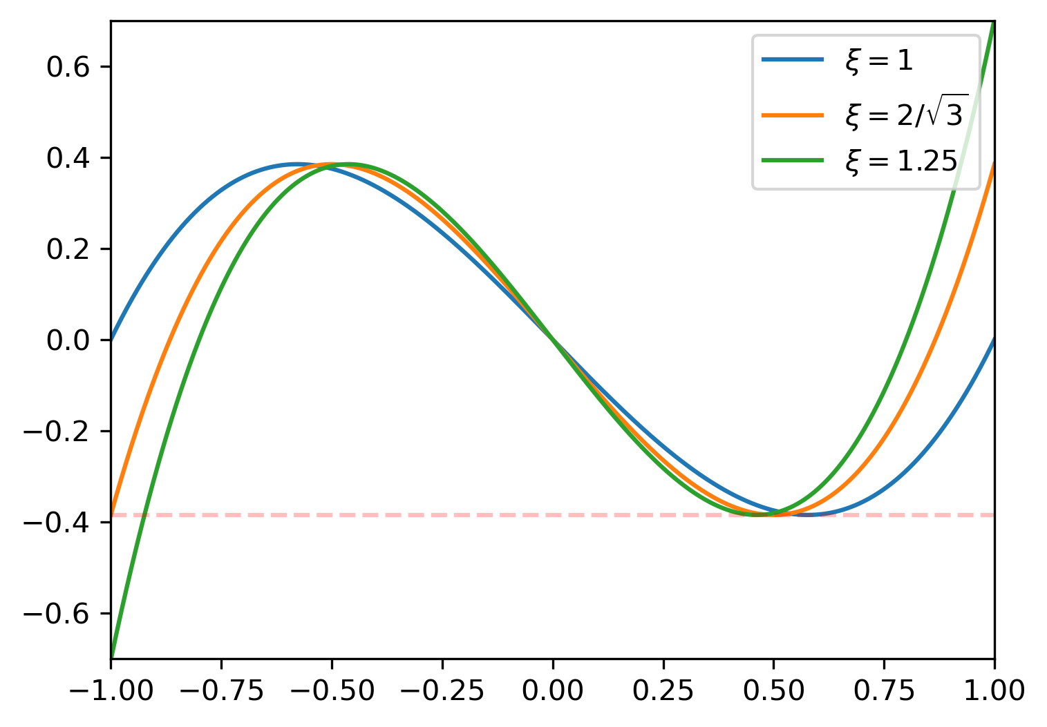
It is clear that any minimal selector would be discontinuous at . Since is analytic in both and , this shows that the smoothness of the objective function does not automatically translate into a smooth dependency of the minimizers with respect to the parameters. As we shall prove in Section 2.2, this issue is intrinsic of minimization problems with nonunique solutions. Thus, we cannot hope, in full generality, for a continuous minimal selection. However, under very mild assumptions, we can at least prove the existence of a measurable selector. Notice that, although this might sound like a minor result, it is still very useful for practical applications. For instance, if is a bounded subset of a given Hilbert space , then a measurable map is automatically an element of the Bochner space for every finite measure over . In fact,
where In particular, one can then reason about suitable ways for approximating via numerical algorithms. In this sense, proving the existence of a measurable selector can be of fundamental interest.
Here, we shall pursue this task by leveraging some basic facts of Set-Valued Analysis, see, e.g., [2]. For better readability, we report them below. In what follows, we recall that a Polish space is a complete separable metric space: in particular, all separable Hilbert spaces are Polish spaces. Hereon, given a set , we shall denote by its power set, that is, the collection of all its possible subsets, namely
Definition 2.1.
Let be a measurable space and let be a Polish space. Let . We say that is a measurable set-valued map if the following conditions hold:
-
a)
is closed in for all ;
-
b)
for all open sets one has , where
(2)
Theorem 2.1 (Kuratowski–Ryll-Nardzewski [2, Th. 8.1.3]).
Let be a measurable space and let be a Polish space. Let be a measurable set-valued map. Then, admits a measurable selection. That is, there exists a measurable map such that for all .
We are now able to state the following result, which proves the existence of a measurable minimal selection.
Theorem 2.2.
Let be a Polish space and let be a compact metric space. Let be lower semi-continuous. Assume that for every the map is continuous. Then, there exists a Borel measurable map such that
Proof.
To start, we note that the statement in the Lemma is well-defined as for all one has
due compactness of and lower semi-continuity of , cf. Lemma 2.1. Let now be the following set-valued map
so that assigns a nonempty subset of to each . We aim at showing that is a measurable set-valued map as in Definition 2.1. Thus, we start by noting that is closed in for all . To see this, fix any and let be defined as . Let We notice that
due minimality. Since is lower semi-continuous, the above ensures that is closed.
Following Definition 2.1, we are now left to show that for any open set , the set
is Borel measurable. To this end, we shall first prove that
| (3) |
Then, our conclusion would immediately follow, as any open set can be written as the countable union of compact sets, , and clearly To see that (3) holds, fix any compact set . Let be a sequence converging to some . By definition of , for each there exists a such that , i.e. for which . Since is compact, up to passing to a subsequence, there exists some such that . Let now be a minimizer for , i.e. a suitable element for which . Since is lower semi-continuous but also continuous in its first argument,
implying that is also a minimizer for . It follows that and thus . In particular, is closed.
All of this shows that fulfills the requirements of Definition 2.1, making it a measurable set-valued map. We are then allowed to invoke the Kuratowski–Ryll-Nardzewski selection theorem, which ensures the existence of a measurable map such that , i.e. .
∎
2.2 Continuity results
As we mentioned previously, the nonuniqueness of the minimizers can often result in the impossibility of a continuous minimal selection, reason for which one is brought to consider weaker notions, such as crude measurability. However, it is natural to ask whether such continuity can be recovered for minimization problems with a unique solution. As we shall prove in a moment, this is actually the case. To this end, we will need the following auxiliary result.
Lemma 2.2.
Let and be metric spaces. A map is continuous if and only if for every and every with the sequence admits a convergent subsequence
Proof.
If is continuous, the statement is obvious. Conversely, assume that for every and every with the sequence admits a convergent subsequence such that We aim to show that is continuous. Let be closed and let be such that for some . By hypothesis, there exists a subsequence . Since and is closed, we have . It follows that . This shows is closed whenever is closed: in other words, is continuous. ∎
We may now prove the following.
Theorem 2.3.
Let and be metric spaces, with compact. Let be lower semi-continuous. Let be defined as
If the marginal is continuous for every , then is continuous. Additionally, if every admits a unique minimizer ,
then the ”argmin map” is continuous.
Proof.
Starting with the first statement, let with . Leveraging compactness, for every , let be such that , cf. Lemma 2.1. We now notice that, since is compact, there exists some and a suitable subsequence such that . Due lower semi-continuity and marginal continuity, for every
| (4) |
It follows that , and thus . In turn, we notice that Eq. (4) then implies
On the other hand, for every and every ,
implying that
Since was arbitrary, passing to the minimum yields
Then and the continuity of follows directly from Lemma 2.2.
As for the second statement in the Theorem, instead, notice that the sequence that we constructed at the beginning of the proof is now . Similarly, due uniqueness, it must be . This proves that for every the sequence admits a subsequence converging to . Once again, the conclusion follows from Lemma 2.2. ∎
We mention that Theorem 2.3 could also be derived from a more general result known as Berge’s Maximum Theorem [4, Chapter 6]. However, stating this properly would require the introduction of additional concepts, such as that of hemicontinuity for set-valued maps. In order to keep the paper self-contained, we refrain from doing so.
3 Preliminaries on low-rank approximation
In this Section we provide a synthetic overview of the fundamental concepts and notions required to properly address the problem of low-rank approximation in Hilbert spaces, going from linear operators (Section 3.1) to random variables (Section 3.2). Specifically, we take the chance to introduce some notation and present the general ideas behind two fundamental algorithms, SVD and POD, that are commonly employed in nonparametric settings.
3.1 Linear operators
We start by introducing some notation. Given a Hilbert space , we denote by the space of bounded linear operators from to . The latter is a Banach space under the operator norm
where is the unit ball. Given any , we define the rank of , and we write , for the dimension of the image . We write , or if clarification is needed, to intend the subspace of consisting of compact operators. Equivalently, see [26, Theorem VI.13],
Following the characterization by Allahverdiev, see [13, Theorem 2.1], given any , we define its th singular value, and we write , as
It is well-known that for all the sequence is bounded, nonincreasing and vanishing to 0 for . Furthermore, We exploit the singular values to introduce the notion of Schatten class operator. Specifically, for all , we set
The latter are all separable Banach spaces under the -norm [8]
For and we obtain two special cases that deserve their own notation. Specifically, for , the operators are said to be of trace class; we shall write to ease notation. For , instead, the operators are said to be of Hilbert-Schmidt type; to emphasize this fact, we shall introduce the notation and . It is well-known that is a Hilbert space on its own [8]. We recall that, for all trace class operators , one has for all orthonormal basis . Furthermore, the quantity
which is commonly referred to as trace of the operator , solely depends on and it is actually independent of the basis [8].
We mention that, for , is the topological dual of , where is the unique value for which
Instead, for , can be characterized as the topological dual of . In all such cases, the duality is realized through the trace operator [8], that is, via the dual product
Here, denotes the adjoint of , that is, the unique operator satisfying for all . It is well known that and share the same singular values; in particular, they belong to the same Schatten class. As a direct consequence, we have the following useful identities concerning the trace norm,
and the Hilbert-Schmidt norm,
3.1.1 Singular Value Decomposition
The SVD, also known as polar form, or canonical form of compact operators, is a powerful tool that allows one to represent compact operators as an infinite series (resp., sum, if the operator has finite rank) of rank-1 operators: see, e.g., [26, Theorem VI.17]. Precisely, if is a compact operator, then one has the representation formula
| (5) |
where , for suitable , and orthonormal sets Notably, are the singular values of . The vectors and are often called the left and right singular vectors of , respectively. If is self-adjoint, then ; in particular, singular values and singular vectors coincide with the notion of eigenvalues and eigenvectors.
From the perspective of low-rank approximation, SVD is extremely interesting as it allows to easily identify optimal low-rank approximants. In fact, one can prove that for every , the best -rank approximation of is given by truncating the series in Eq. (5) at For later reference, we formalize this fact in the Lemma right below, which is ultimately a more abstract version of the well-known Eckart-Young Lemma [10]. Given that the infinite-dimensional case is rarely discussed in detail, the interested reader can find a corresponding proof in B.
Lemma 3.1.
Let be a separable Hilbert space. Let . There exists two orthonormal sequences, and , such that
Additionally, for every , the truncated operator satisfies
| (6) |
as well as,
| (7) |
Furthermore, if and , then is the unique minimizer of (7).
3.2 Hilbert-valued random variables
We now move to low-rank approximation of Hilbert-valued random variables. As in the previous case, we start by recalling some fundamental concepts and introducing the proper notation. Let be a separable Hilbert space. Given a probability space , where is the sample space, a suitable sigma algebra defined over , and a probability distribution, an -valued random variable is a Borel measurable map
For any exponent , it is custom to introduce the -valued spaces, here denote as
where is the expectation operator, defined with respect to The latter are all separable Banach spaces under the Bochner norm222Note: up to the usual identification given by the equivalence relation -almost surely.
as soon as the probability space is itself separable; that is, if the metric makes a separable topological space.
Before proceeding further, we mention a few relevant facts about these spaces. The first one, is about the standard inclusion, holding for all The second one concerns the duality , with , realized by the inner product
Finally, by leveraging the theory of Bochner integrals [32, Chapter V.5], one can also introduce the concept of -valued expectation. Namely, for any , one can prove that there exists a unique element in , denoted as , such that
The latter is called expected value of .
Remark 3.1.
Hereon, the existence of the probability space will be omitted. That is, we will simply say that is an -valued random variable, without specifying the underlying probability space (which, for simplicity, we always assume to be complete). Clearly, when considering spaces, the probability space is intended to be the same for all -valued random variables under study.
3.2.1 Principal Orthogonal Decomposition
As we mentioned in the introduction, POD is popular technique for reducing the complexity of high-dimensional random variables. From an abstract point of view, the construction underpinning the POD is based on a truncated series expansion. The idea, in fact, is that all square-integrable Hilbert-valued random variable admit a series representation of the form
where is a nonincreasing sequence of positive scalar numbers, is an orthonormal basis of the Hilbert state space , whereas is an -orthonormal sequence of scalar valued random variables, meaning that We mention that, if for a suitable spatial domain , then can be considered a random field, and the series expansion is often referred to as ”Kosambi-Karhunen-Loève expansion”.
It is worth highlighing the fact that, although one has almost surely for any orthonormal basis , optimal representations are only obtained for special choices of the basis vectors (which, ultimately, depend on ). In fact, in most cases the random variables would yield . In particular, if , this would result in a statistical correlation between the coefficients in the series expansion.
As a matter of fact, it is this avoidance of redundances that makes the Kosambi-Karhunen-Loève expansion a useful tool for low-rank approximation. In fact, given a reduced dimension , one can prove the following optimality of the truncated series expansion (and, thus, of the POD),
where A more rigorous statement can be found in the Lemma right below. As before, being the following a classical result, we defer the proof to the B.
Lemma 3.2.
Let be a separable Hilbert space. Given a square-integrable -valued random variable , i.e. , let be the linear operator
where the integral is understood in the Bochner sense. Then:
-
i)
in a symmetric positive semidefinite trace class operator;
-
ii)
there exists a sequence of (scalar) random variables with such that
almost surely, where and are the eigenvalues and eigenvectors of , respectively;
-
iii)
for every orthogonal projection one has
-
iv)
for every the random variable satisfies
where
4 Parameter dependent low-rank approximation
We are now ready to address the case of parameter dependent low-rank approximation. To start, we shall derive some general results about the dependency of singular values and singular vectors with respect to the underlying operator. Then, we will split our presentation in two parts, concerning parametric SVD and parametric POD, respectively.
We mention that, throughout the whole Section we will need to use basic facts of Functional Analysis concerning weak topologies. To this end, we recall that, given a Hilbert space the weak topology is the coarsest topology that makes the linear functionals continuous for all . To distinguish between convergence in the strong (i.e., norm) topology and the weak topology, we will use the notation and , respectively. We also recall that: all convex sets are strongly closed if and only if they are weakly closed; all weakly closed sets that are norm bounded are weakly compact (and metrizable, if is separable); all weakly convergent sequences are norm bounded; compact operators map weakly convergent sequence into strongly convergent ones; the weak and strong topology induce the same Borel sigma-field, cf. Lemma A.2 in A.
4.1 General results
We start by presenting some general results concerning the dependence of singular values and singular vectors on the underlying operator. Roughly speaking, the former are better behaved, as they are characterized by a continuous dependency, while the latter can be subject to discontinuities. To see this, consider the following example of a parameter dependent matrix,
where Due symmetry, singular values and singular vectors coincide with eigenvalues and eigenvectors, respectively. Since is the largest singular value, we have
Similarly, if and otherwise. Both and are continuous. However, the corresponding eigenvectors are
both of which depend discontinuously on Clearly, the issue is caused by the branching point , where . From an intuitive point of view, this is not really surprising. This whole phenomenon, in fact, is strictly related to the one discussed in Section 2: indeed, we can think of singular values and singular vectors as minimum values and minimizers of suitable minimization problems. Then, it becomes evident that changes in multiplicites of the eigenvalues can produce discontinuities in the dependency of singular vectors. Still, by leveraging the results in Section 2, we may at least trade continuity with measurability. We detail our reasoning right below, starting with the case of singular values and them moving to singular vectors.
Theorem 4.1.
Let be a separable Hilbert space. Let be the space of compact operators from to . Fix any . The map is 1-Lipschitz continuous. That is, for all one has
Proof.
Let and . Fix any . By definition, there exists some with such that . We have
Since was arbitrary, we deduce . Due symmetry in and , the conclusion follows. ∎
Theorem 4.2.
Let be a separable Hilbert space and let be the space of compact operators from to . Fix any . There exists a Borel measurable map from , mapping
such that, for every ,
-
i)
and for all ;
-
ii)
minimizes the -rank truncation error, i.e.,
-
iii)
and for all ;
-
iv)
for all with one has ;
-
v)
the optimality in (ii) holds also with respect to the Hilbert-Schmidt norm;
-
vi)
if then for all with
Proof.
We subdivide the proof into multiple steps. In what follows, let be the closed unit ball and let Let be the weak topology over and let .
Step 1.
The functional acting as
is: i) marginally continuous in ; ii) lower-semicontinuous.
Proof.
The first statement is a direct consequence of Theorem 4.1. As for the lower semi-continuity, instead, let , and . Then, for every , , we have
due continuity of the singular values. It follows that
since strongly. Consequently, if
Passing at the supremum over yields
| ∎ |
Step 2.
The functional acting as
is: i) marginally continuous in ; ii) lower-semicontinuous.
Proof.
As previously, the first statement comes directly from Theorem 4.1. As for the second one, instead, let , and . We have
since is uniformly norm bounded and turns weak convergence into strong convergence. Thus, meaning that strongly. In particular, due continuity of the singular values, . Since is lower-semicontinuous in the weak topology, the conclusion follows. ∎
Step 3.
The functional acting as
is continuous.
Proof.
Let and . As before, we have strongly due compactness of . Since is continuous in , the conclusion follows. ∎
Step 4.
The functional acting as
is: i) marginally continuous in ; ii) lower-semicontinuous.
Proof.
We recall that implies Then, the statement follows from Steps 2-3. ∎
Step 5.
Statements (i)-(iv) in Theorem 4.2 hold true.
Proof.
Consider the functional defined as
which, by the previous steps, is lower-semicontinuous in and continuous in for every We notice that, for every ,
In addition, for every , one can leverage the classical SVD to construct a list that minimizes all four functionals simultaneously: due optimality of the truncated SVD, cf. Lemma 3.1, due definition of singular vectors, thanks to the orthogonality constraints,
and similarly for , since . Clearly, is not unique as, for instance, . Nonetheless, this shows that
Then, leveraging the continuity properties of and the compactness of , let be a Borel measurable selector such that for all , cf. Theorem 2.2 and Lemma A.2. For better readability, write Then, we notice that, implies
-
, thus . This is part of (i) in the Theorem;
-
, which is (ii) in the Theorem;
-
and by definition of , thus ensuring (iii);
-
and, by the previous observation,
In particular, if then and the above yields . This is part of (iv) in the Theorem;
-
ensuring the equivalent conditions on the adjoint and thus proving (i) and (iv). ∎
Step 6.
Statements (v)-(vi) in Theorem 4.2 hold true.
Proof.
Thanks to (i)-(iii), the vectors and are guaranteed to be left and right singular vectors of , respectively, whenever . In particular, the operator is a truncated SVD of , and (v) automatically follows from Lemma 3.1. Finally, to prove (vi) notice that if then
meaning that is an eigenvector of . However, since is a symmetric operator, and are known to share the same eigenvectors. Then, it must be Dividing by yields the desired conclusion. ∎ ∎
Remark 4.1.
As a direct consequence of Theorems 4.1 and 4.2, it is evident that there exists a measurable map that, for a fixed dimension , maps each onto a corresponding optimal low-rank approximant (according to the operator norm). Similarly, there also exists a measurable map that assigns each onto an optimal low-rank approximant defined according to the Hilbert-Schmidt norm. Interestingly, it the latter case, by leveraging Theorem 2.3 combined with the uniqueness result in Lemma 3.1, one can actually prove that the restriction of such map to the open subset is continuous. Here, however, we shall discuss this fact directly in Section 4.2 when considering the parametric scenario.
4.2 Parametric SVD
Theorem 4.3.
Let be a measurable space and let be a separable Hilbert space. Let the space of compact operators from to . Let be a measurable map. Fix any . Assume that for all . Then, there exists measurable maps
such that , and
for all Furthermore, if is in fact a topological space and depends continuously on , then the maps are be continuous. The same results hold if is replaced with and the operator norm is substituted by the Hilbert-Schmidt norm.
Proof.
In general, looking for a continuous analogue of Theorem 4.3 can be nontrivial. This is also because the series representation presents some intrinsic redundancies. For instance, it is clear that replacing and with and would yield exactly the same result. Instead, a more intuitive approach is to directly search for a map that given returns an optimal -rank approximant of : see also the forthcoming discussion in Section 4.3.2. If we adopt this change in perspective, then, it is not hard to prove the following.
Theorem 4.4.
Let be a compact metric space and let be a separable Hilbert space. Let be the space of Hilbert-Schmidt operators from to . Let be continuous. Fix any . Assume that
Then, there exists a continuous map such that, for every , the operator is the best -rank approximation of in both the operator norm and the Hilbert-Schmidt norm.
Proof.
Let . We shall prove that is sequentially weakly-closed in . Let . We have for suitable and orthonormal sets and . Since , the sequence must be norm bounded in . It follows that for some constant uniformly in and . Similarly, . Then, up to passing to a suitable subsequence, due compactness of and weak-compactness of the unit ball in , we have , and for some , and . In particular, for every ,
meaning that , and thus due uniqueness of the weak limit. Next, we notice that due compactness of and continuity of the parametrization,
Let . It is well-known that is weakly-compact and metrizable. In particular, so is the subset . Then, let be a metric over compatible with the weak topology over . Consider the functional given by
Clearly, is continuous in . Furthermore, it is also lower-semicontinuous since the Hilbert-Schmidt norm is weakly lower-semicontinuous from and whenever and . Next, notice that for every , the operator admits a unique minimizer of within , which is given by the truncated SVD: in fact, this is a direct consequence of the uniqueness result in Lemma 3.1. Since all the assumptions in Theorem 2.3 are satisfied, it follows that the map is continuous. To conclude, we notice that if then
by continuity of the singular values. Since is a Hilbert space, and thus possesses the Radon-Riesz property, the above convergence, combined with the previously shown weak convergence, ensures that strongly. In other words, the map is continuous, as claimed. Finally, since is actually the truncated SVD of , the optimality in the operator norm descends directly from Lemma 3.1. ∎
Remark 4.2.
Compared to Theorem 4.3, the continuity result in Theorem 4.4 requires two additional assumptions. The first one is that the parametrization is continuous, which is clearly a necessary condition. The second one, instead, is an assumption of ”uniform non-branching”. In fact, we require that for every . As made evident by our discussion at the beginning of Section 4, this assumption is essentially fundamental, and it boils down to eluding the branching phenomenon typical of minimization problems, cf. Section 2.1. In fact, similar conditions are also required when studying higher regularity results: see, e.g., the literature on perturbation theory of linear operators [19]. As a side note, we remark that the non-branching condition only concerns . The remaining singular values, instead, are allowed to change their multiplicities as varies.
4.3 Parametric POD
We now switch from linear operators to high-dimensional random variables, with the purpose of deriving basic regularity results for parametric POD. In this case, we shall present two results. The first one discusses the measurability of parametric POD, and it is obtained under very mild assumptions. The second one, instead, is a continuity result, derived under a suitable no-branching condition. The two are discussed in Sections 4.3.1 and 4.3.2, respectively.
4.3.1 Measurability results
We start with the following measurability result for parametric POD, which ultimately descends from Theorem 4.3.
Theorem 4.5.
Let be a measurable space and let be a separable Hilbert space. Let be a family of square-integrable Hilbert-valued random variables. Assume that the map is measurable from . Fix any There exists measurable maps
such that and
for all where
Furthermore, if is a topological space and for , then the maps are continuous.
Proof.
Fix any . Let ,
be the —uncentered— covariance operator of . Let and be the eigenvalues and eigenvectors of , sorted such that Set . Then, as we discussed in Lemma 3.2, it is well-known that the random variable
minimizes within . We now notice that, since , and embedds continuously in , by Theorem 4.3 there exist measurable maps and such that
The first statement in the Theorem follows. Finally, we notice that if for , then the map is actually continuous. Since
and depends continuously on through (see, e.g., Lemma A.3 in A) the conclusion follows. ∎
We conclude this subsection with an application of Theorem 4.5 to the context of random fields, where each realization of the random variable is in fact a function, or a trajectory, defined over a suitable spatial domain. Specifically, we focus on the case in which for some measurable set In this case, rather than introducing measurable maps , we directly frame the result in terms of multi-variable functions , which better reflects the notation commonly adopted in the literature. Similarly, re-write the low-rank approximant using the classical formula derived from the Kosambi-Karhunen-Loève expansion.
Corollary 4.1 (Parametric Kosambi-Karhunen-Loève expansion).
Let be a measurable space and let be Lebesgue measurable. Let be a family of stochastic processes defined over . Assume that
for all Additionally, assume that the map is measurable. Then, there exists measurable maps
and a family of random variables such that and
for all where
Furthermore, if is a topological space and for , then the maps are continuous.
Proof.
This is just Theorem 4.5 with . The latter, in fact, yields the existence of suitable measurable maps such that and
Then, letting and
yields
The only caveat concerns defining the maps such that almost everywhere in . In fact, pointwise evaluations of functions are a delicate matter, and we cannot simply set However, we can easily circumvent this problem by defining
Notice that, being the pointwise limsup of measurable maps, this guarantees the maps to be measurable. Furthermore, if we denote by the hypercube of edge length centered at , we see that
In particular, by Lebesgue differentiation theorem,
| ∎ |
4.3.2 Continuity results
Following our discussion in Section 2, it is natural to ask whether additional assumptions may lead to an improved regularity of the parametric POD, possibly stepping up from measurability to continuity. In this concern, one must be careful in defining the map of interest. For instance, if we insist on parametrizing single vectors in the low-rank approximation, , things become unnecessarily complicated. This is because the quality of the approximation is not related to the vectors themselves, but rather to the underlying subspace.
For instance, notice that, given any , replacing with any orthonormal basis of
would leave the low-rank approximant in Theorem 4.5 unchanged. In fact, the latter is just the projection of onto . In this sense, it would be more appropriate to focus our attention on the map , as to avoid redundances. Furthermore, this change of perspective has a better potential of bringing continuity into the game. In fact, as we discussed in Section 2, when it comes to optimal solutions of parametric problems, there is an intimate connection between continuity and uniqueness.
To simplify our analysis, however, we shall identify all subspaces with their corresponding orthonormal projector . In this way, topological notions, such as continuity, compactness, closure, etc., will not require additional concepts (such as that of Grassmann manifold [3, 11]), instead, they will descend directly from the theory of linear operators. In this concern, notice that, since , all such operators are members of the Schatten class , for any . Here, we shall leverage the case , as it is the one with the most remarkable mathematical structure (Hilbert case). We report our main result below. The attentive reader will notice that the proof is fundamentally a re-adaptation of the ideas presented in the proofs of Theorem 4.4 and Lemma 3.1.
Theorem 4.6.
Let be a metric space and let be a separable Hilbert space. Let be a family of square integrable -valued random variables. Assume that the map is continuous from . Fix any and let
where is the unit ball. For every let be the (uncentered) covariance operator
and be its largest eigenvalues, . If, for every , one has the strict inequality
then, there exists a continuous map , mapping , such that
| (8) |
for all
Proof.
We subdivide the proof into multiple steps, each consisting of a claim and a corresponding proof.
Step 1.
is weakly closed in .
Proof.
Let be weakly convergent to some . Let be such that . Due boundness, up to passing to a subsequence, there exists such that . Let . For every , , we have
meaning that . Due uniqueness of the limit, , meaning that , as claimed.∎
Step 2.
The weak topology of makes a compact metric space.
Proof.
Since is a separable Hilbert space itself, all balls are weakly compact and metrizable under the weak topology. Therefore, in light of Step 1, it suffices to show that is norm bounded. To this end, we note that for every one has
| ∎ |
Step 3.
The functional given by
is lower semi-continuous with respect to the product topology , with being the weak topology induced by .
Proof.
Let and . As we argued previously, without loss of generality we may write
with . For every we have
For each term oh the r.h.s., we have . In fact,
The first term goes to zero due dominated convergence, since almost-surely and , as , which has finite moment; conversely, the second term is infinitesimal as it equals
It follows that , and thus, in . In particular, and, consequently,
as wished. ∎
Step 4.
If is an orthonormal projector, then
where and are the eigenvalues and eigenvectors of , respectively.
Proof.
This is just (iii) of Lemma 3.2. ∎
Step 5.
For all there exists a unique minimizing .
Proof.
Fix any and let . Let Now, let be an orthonormal basis of and define . Since and both map onto , due optimality of orthogonal projections, we have
for all It follows that . That is to say: all minimizers of are —without loss of generality— given by orthogonal projections. Let and be the eigenvalues and eigenvectors of . By Step 4, we know that for all orthonormal projectors we have
Then, minimizes if and only if it maximizes Since
any yielding for and for is guaranteed to be a maximizer (resp., minimizer for ), cf. Lemma A.1 in A. However, it is straightforward to see that this is possible if and only if is the orthonormal projection onto ∎
Step 6.
Theorem 4.6 holds true.
Proof.
In light of Steps 1-5 and Theorem 2.3, there exists a map , satisfying Eq. (8), which is continuous from . Thus, we only need to prove that the continuity of this map is fact stronger, holding in the topology of the Hilbert-Schmidt norm. To this end, we simply note that for we have but also
since for all (cf. Step 5). Since and is a Hilbert space, this suffices to show that strongly, as claimed. ∎ ∎
5 Corollaries for parametric approximation
In this Section, we derive a few Corollaries for practical applications that deal with parametric low-rank approximation. As we discussed in the Introduction, this step is essential since parametric SVD and parametric POD can be too expensive to compute. To simplify, let us reduce to the finite-dimensional case. Consider, for instance, the problem of dimensionality reduction for a family of random variables taking values in . Under suitable assumptions, Theorems 4.5-4.6 ensure the existence of suitable projectors , of rank , that minimize the truncation error However, for each , computing requires the solution of an eigenvalue problem. To avoid this complication, we might seek for another map, , cheaper to evaluate, and such that Typically, the surrogate is to be sought in a suitable hypothesis space
In general, the smoother the dependency of on , the easier we expect the construction of the surrogate model to be (or the stronger its resemblance with the ideal optimum). Clearly, the hypothesis space needs also to be sufficiently rich. For instance, if the ideal parametric approximation is continuous, then should be dense in , the space of continuous maps from , here endowed with the norm
Conversely, if is merely measurable, then, given a finite measure over , a good choice could be to look for hypothesis spaces that are dense in , the Bochner space of -integrable functions from , the latter being equipped with the norm
In particular, if for some , then neural network models can be an interesting choice (and, in fact, numerical algorithms based on these ideas have recently emerged, cf. [5, 12]). This is because, having fixed any continuous nonpolynomial activation function, the set of neural network architectures from is dense both in and . This is a direct consequence of the so-called universal approximation theorems: see, e.g., [16].
We mention that similar principles hold for the case of parametric low-rank approximation of linear operators. With these considerations in mind, we may now state the following results. In order to keep the paper self-contained, all proofs are postponed to C.
Corollary 5.1.
Let be a finite measure space and let . Let be a measurable map such that
Fix any integer . Assume that for all . Let and be dense subsets of the respective superset. Then, for every , there exists and such that
Corollary 5.2.
Let be a compact metric space and let . Let be continuous. Assume that for all Let be the closed subset of matrices with rank smaller or equal to . Let be dense. Then, for every there exists some such that
for all
Corollary 5.3.
Let be a finite measure space and let . Let be a family of random variables in with finite second moment. Assume that the map is measurable and
For every , let be the eigenvalues of the uncentered covariance matrix Fix any integer and let be a dense subset. Then, for every there exists some such that
Corollary 5.4.
Let be a compact metric space and let . Let be a family of random variables in with finite second moment. Assume that
For every , let be the eigenvalues of the uncentered covariance matrix Fix any integer and let be the closed subset of matrices with rank smaller or equal to . Let be a dense subset. If for every , then, for every there exists some such that
6 Conclusions
In this work, we presented a unified framework for parametric low-rank approximation, covering applications ranging from numerical analysis (such as the approximation of linear operators) to probability and statistics (such as the dimensionality reduction of Hilbert-valued random variables). Additionally, we established foundational results regarding the regularity of parametric algorithms, including parametric SVD and parametric POD, in terms of measurability and continuity, with implications for learning algorithms relying upon universal approximators.
Our results, derived under extremely mild assumptions, are nearly as general as possible. This distinguishes our analysis from other fields, such as perturbation theory, which typically focuses on small parametric variations and specific regimes where singularities and discontinuities are less likely to occur.
We framed our discussion within the context of separable Hilbert spaces, which makes our analysis applicable to both finite and infinite-dimensional problems. Extending our theory to separable Banach spaces is of interest but not straightforward due to the absence of a canonical form for compact operators. Furthermore, this extension will likely require different analytical tools, as our construction can at most generalize to Banach spaces admitting a pre-dual. In fact, our arguments often require some form of compactness, for which the weak* topology becomes an essential ingredient. Furthermore, certain proofs, such as the one in Theorem 4.6, would require additional assumptions concerning reflexivity and the Radon-Riesz property.
Another intriguing research direction is to explore higher regularity properties, such as the Lipschitz continuity and differentiability of parametric SVD and parametric POD. From an applicative standpoint, this could lead to more practical insights regarding universal approximators, allowing, for instance, to discuss the computational complexity of the approximating algorithms, rather than their existence alone, as seen in [16]-[31].
Declarations
Acknowledgements
The present research is part of the activities of project ”Dipartimento di Eccellenza 2023-2027”, funded by MUR, and of ”Gruppo Nazionale per il Calcolo Scientifico” (GNCS), of which the author is member. The author would also like to thank Simone Brivio for inspiring the development of this work, Prof. Paolo Zunino for his precious support, and Dr. Jacopo Somaglia for the insightful discussions that indirectly contributed to this research.
Funding
The author has received funding under the project Cal.Hub.Ria (Piano Operativo Salute, traiettoria 4), funded by MSAL.
Conflict of interest
The author declares to have no competing interests.
Appendix A Auxiliary results
Lemma A.1 (Truncation Lemma).
Let . Let be such that
for some . Let , and consider the linear functional ,
All maximizers satisfy and In particular, if , then admits a unique maximizer within , obtained by setting for all and for all
Proof.
Notice that is both closed and convex. Consequently, since is the topological dual of , classical arguments of weak∗-compactness show that admits one or more maxima over . Now, let be such that . Then, there exists two indexes, and such that
Let and define the sequence
It is straightforward to see that . We have
since . Therefore, is not a maximizer of . This shows that any maximizing must satisfy , as claimed. Finally, we notice for all . Thus, for any maximizing we have
since for all By leveraging the fact that for , and by repeating the same argument as before, it is straightforward to see that, without loss of generality we may focus on those maximizers for which Then, these satisfy for all , and, thus It follows that ∎
Corollary A.1.
Let be a separable Hilbert space. Let be given in canonical form as Fix any . For all orthonormal sets one has
| (9) |
Additionally, if , then the equality can be realized if and only if .
Proof.
Let Let be the orthogonal projection from onto . Clearly, and, in particular, We have
Now, let By definition, and Then, Eq. (9) follows directly from Lemma A.1. Similarly, if , Lemma A.1 ensures that the equality can be achieved if and only if for all and for all Equivalently, must be the projection onto . The conclusion follows. ∎
Lemma A.2.
Let be a separable Hilbert space. Let and be the strong and weak topologies over , respectively. Then, and induce the same Borel sigma-field.
Proof.
Let and be the sigma-algebras generated by the two topologies. Since , we have . Let and . Notice that, for every , the strongly closed ball is also weakly closed. It follows that for every , and thus
This proves that every strongly open ball in lies in . It follows that and thus . ∎
Lemma A.3.
Let be a separable Hilbert space, endowed with a suitable probability measure Let be two -valued random variables such that . Let be the (uncentered) covariance operators, and , respectively. Then,
Proof.
Let with and fix any orthonormal basis . We have
By applying the triangular inequality, we get
Notice that the two terms are symmetric in and , thus, it suffices to study one of the two. For instance, focusing on the first one yields
Since , it follows that
and thus Passing at the supremum over yields the conclusion. ∎
Appendix B Proofs of Section 3
Proof of Lemma 3.1
Proof.
Let be a separable Hilbert space and let be a compact operator. We aim to prove that admits a series expansion of the form for two orthonormal basis and intrinsically depending on . Then, we plan to prove that the truncated series yields the best -rank approximation of in both the operator norm and the Hilbert-Schmidt norm. Finally, is the unique minimizer in the Hilbert-Schmidt case whenever strictly. We may now begin the proof.
As we mentioned, the series representation is a well-known result often referred to as the ”canonical form of compact operators”, see, e.g.
[26, Theorem VI.17]. Concerning the optimality of the truncated SVD in the operator norm, instead, we simply notice that for every one has
| (10) |
due monotonicity of the singular values. It follows that
Since , the conclusion follows. Let us now discuss the case of the Hilbert-Schmidt norm. Notice that with implies . In particular, if then (7) is obvious since and thus , coherently with the fact that must diverge. Instead, assume that . We can leverage a Von Neumann type inequality, which states that for any one has , cf. [9]. As a direct consequence, see, e.g., [15, Corollary 7.4.1.3],
We now notice that if , then for all , as clearly seen by expanding in its canonical form. It follows that, in this case,
as claimed. The above also shows that any -rank operator minimizing must satisfy for all In particular, and must share the same singular values. In light of this fact, let . We have
In particular, must be such that is maximized. To this end, let be an orthonormal basis for , where , so that forms an orthonormal basis of Since for all , we have,
It follows that
the last inequality coming from Corollary A.1. On the other hand, the upper-bound is reached whenever , thus, if is actually a maximizer of , the above needs to be an equality. In turn, this implies that , once again by Corollary A.1. In particular, since and coincide on , we may re-write as
On the other hand, due minimality (resp. maximality) it must be
Now recall that . Since is a Hilbert space, due uniform convexity, there is a unique element in which maximizes , which is precisely It follows that , as claimed. ∎
Proof of Lemma 3.2
Let be a separable Hilbert space and let be a square-integrable -valued random variable with a given probability law . Let be the linear operator We prove the following.
-
i)
in a symmetric positive semidefinite trace class operator.
Proof.
We notice that, for all , we have
In particular, for , Thus, having fized any orthonormal basis , we may compute as
∎ -
ii)
There exists a sequence of (scalar) random variables with such that -almost surely, where and are the eigenvalues and eigenvectors of , respectively.
Proof.
Let It is straightforward to see that for all one has
Finally, it is clear that by definition.∎
-
iii)
For every orthogonal projection one has
Proof.
Let be an orthogonal projection and let . Let be an orthonormal basis of , be it finite or infinite depending on the dimension of Due orthogonality,
Expanding the second term, due -orthonormality of the and orthonormality of the ’s, reads,
-
iv)
For every the random variable satisfies where
Proof.
Fix any Let be a subspace of dimension such that -almost surely. Let denote the orthogonal projection onto . Due optimality of orthogonal projections, we have
the equality following from point (iii). Now, let , and let be an orthonormal basis for . Without loss of generality, extend the latter to a complete orthonormal basis, , spanning the whole . We notice that and
Therefore, as a direct consequence of Lemma A.1,
Since is easily shown to equal , the conclusion follows. ∎
Appendix C Proofs of Section 5
Proof of Corollary 5.1
Let . Since we are in a finite dimensional framework, all matrices in can be seen as compact operators . Let
be the maps in Theorem 4.3. Then, , . Furthermore, if we set
then
for all Clearly, are all measurable in by composition. Furthermore, since and for all , it follows that
since and by assumption. Fix any . Leveraging the density assumption, let and be such that
By recalling that and for any two compatible matrices , one can easily prove via the triangular inequality that for every
| (11) | ||||
| (12) | ||||
| (13) |
We now notice that, if are measurable functions, by repeated Hölder inequality
Then, integrating Eq. (11) and applying the above yields
| (15) |
where
having also exploited the fact that, by triangular inequality in and ,
and
Now, fix any and let be such that the right-hand-side of Eq. (15) is strictly bounded by . By triangular inequality,
as claimed.∎
Proof of Corollary 5.2
Let . Analogously to the proof of Corollary 5.1, this time we notice that all the assumptions in Theorem 4.4 are satisfied. Consequently, there is a map such that
| (16) |
for all . Let . Leveraging density, let be such that
To this end, notice that, since we are in finite-dimensional setting, is dense irrespectively of whether we endow the output space with the operator norm or the Hilbert-Schmidt norm. Since , the above, combined with Eq. (16), directly yields the desired conclusion via the triangular inequality.
Proof of Corollary 5.3
Let . Being in the position to invoke Theorem 4.5, let be such that
Let . Since is orthonormal, . In particular, Leveraging density, let be -close to . Notice that, pointwise in and in the probability space, we have
We can bound the second term as
Integrating the above over the probability space and over then yields
via repeated Hölder inequality. Here,
so that via triangular inequality. Then, for , we have
| (17) |
Clearly, for every , there exists some for which the above is bounded by Finally, recall that, by construction,
| (18) |
Proof of Corollary 5.4
Let . We notice that all the assumptions in Theorem 4.6 are fullfilled. In particular, there exists a continuous map such that
for all where Given any , leveraging the density of in , let be such that
For every we have
where due continuity of and compactness of the parameter space Then, choosing immediately yields the conclusion.∎
References
- [1] David Amsallem and Charbel Farhat. Interpolation method for adapting reduced-order models and application to aeroelasticity. AIAA journal, 46(7):1803–1813, 2008.
- [2] Jean-Pierre Aubin and Hélène Frankowska. Set-valued analysis. Springer Science & Business Media, 2009.
- [3] Thomas Bendokat, Ralf Zimmermann, and P-A Absil. A grassmann manifold handbook: Basic geometry and computational aspects. Advances in Computational Mathematics, 50(1):1–51, 2024.
- [4] Claude Berge. Topological spaces: Including a treatment of multi-valued functions, vector spaces and convexity. Oliver & Boyd, 1877.
- [5] Jules Berman and Benjamin Peherstorfer. Colora: Continuous low-rank adaptation for reduced implicit neural modeling of parameterized partial differential equations. arXiv:2402.14646, 2024.
- [6] Angelika Bunse-Gerstner, Ralph Byers, Volker Mehrmann, and Nancy K Nichols. Numerical computation of an analytic singular value decomposition of a matrix valued function. Numerische Mathematik, 60:1–39, 1991.
- [7] Hervé Cardot. Conditional functional principal components analysis. Scandinavian journal of statistics, 34(2):317–335, 2007.
- [8] John B Conway. A course in functional analysis, volume 96. Springer, 2019.
- [9] Gunther Dirr and Frederik vom Ende. Von neumann type of trace inequalities for schatten-class operators. Journal of Operator Theory, 84(2):323–338, 2020.
- [10] Carl Eckart and Gale Young. The approximation of one matrix by another of lower rank. Psychometrika, 1(3):211–218, 1936.
- [11] Alan Edelman, Tomás A Arias, and Steven T Smith. The geometry of algorithms with orthogonality constraints. SIAM journal on Matrix Analysis and Applications, 20(2):303–353, 1998.
- [12] Nicola Rares Franco, Andrea Manzoni, Paolo Zunino, and Jan S Hesthaven. Deep orthogonal decomposition: a continuously adaptive data-driven approach to model order reduction. arXiv:2404.18841, 2024.
- [13] Israel Gohberg and Mark Grigor’evich Kreĭn. Introduction to the theory of linear nonselfadjoint operators, volume 18. American Mathematical Soc., 1978.
- [14] Ajay Gupta and Adrian Barbu. Parameterized principal component analysis. Pattern Recognition, 78:215–227, 2018.
- [15] Roger A Horn and Charles R Johnson. Matrix analysis. Cambridge university press, 2012.
- [16] Kurt Hornik. Approximation capabilities of multilayer feedforward networks. Neural networks, 4(2):251–257, 1991.
- [17] Ian T Jolliffe. Principal component analysis: a beginner’s guide—i. introduction and application. Weather, 45(10):375–382, 1990.
- [18] Kari Karhunen. Under lineare methoden in der wahr scheinlichkeitsrechnung. Annales Academiae Scientiarun Fennicae Series A1: Mathematia Physica, 47, 1947.
- [19] Tosio Kato. Perturbation theory for linear operators, volume 132. Springer Science & Business Media, 2013.
- [20] DD Kosambi. Statistics in function space. DD Kosambi: Selected Works in Mathematics and Statistics, pages 115–123, 2016.
- [21] Beatriz Lafferriere, Gerardo Lafferriere, and Mau Nam Nguyen. Introduction to Mathematical Analysis I. Portland State University Library, 2022.
- [22] Eleonora Musharbash, Fabio Nobile, and Tao Zhou. Error analysis of the dynamically orthogonal approximation of time dependent random pdes. SIAM Journal on Scientific Computing, 37(2):A776–A810, 2015.
- [23] Efe A Ok. Real analysis with economic applications, volume 10. Princeton University Press, 2007.
- [24] Alfio Quarteroni, Andrea Manzoni, and Federico Negri. Reduced basis methods for partial differential equations: an introduction, volume 92. Springer, 2015.
- [25] JO Ramsay and BW Silverman. Principal components analysis for functional data. Functional data analysis, pages 147–172, 2005.
- [26] Michael Reed and Barry Simon. Methods of modern mathematical physics. vol. 1. Functional analysis. Academic San Diego, 1980.
- [27] Themistoklis P Sapsis and Pierre FJ Lermusiaux. Dynamically orthogonal field equations for continuous stochastic dynamical systems. Physica D: Nonlinear Phenomena, 238(23-24):2347–2360, 2009.
- [28] John R Singler. New pod error expressions, error bounds, and asymptotic results for reduced order models of parabolic pdes. SIAM Journal on Numerical Analysis, 52(2):852–876, 2014.
- [29] Nancy L Stokey and Robert E Lucas Jr. Recursive methods in economic dynamics. Harvard University Press, 1989.
- [30] REL Turner. Perturbation with two parameters. Linear Algebra and its Applications, 2(1):1–11, 1969.
- [31] Dmitry Yarotsky. Error bounds for approximations with deep relu networks. Neural Networks, 94:103–114, 2017.
- [32] Kôsaku Yosida. Functional analysis, volume 123. Springer Science & Business Media, 2012.