Convergence rate of opinion dynamics with complex interaction types
Abstract
The convergence rate is a crucial issue in opinion dynamics, which characterizes how quickly opinions reach a consensus and tells when the collective behavior can be formed. However, the key factors that determine the convergence rate of opinions are elusive, especially when individuals interact with complex interaction types such as friend/foe, ally/adversary, or trust/mistrust. In this paper, using random matrix theory and low-rank perturbation theory, we present a new body of theory to comprehensively study the convergence rate of opinion dynamics. First, we divide the complex interaction types into five typical scenarios: mutual trust , mutual mistrust , trustmistrust , unilateral trust , and unilateral mistrust . For diverse interaction types, we derive the mathematical expression of the convergence rate, and further establish the direct connection between the convergence rate and population size, the density of interactions (network connectivity), and individuals’ self-confidence level. Second, taking advantage of these connections, we prove that for the , , , and random mixture of different interaction types, the convergence rate is proportional to the population size and network connectivity, while it is inversely proportional to the individuals’ self-confidence level. However, for the and scenarios, we draw the exact opposite conclusions. Third, for the and scenarios, we derive the optimal proportion of different interaction types to ensure the fast convergence of opinions. Finally, simulation examples are provided to illustrate the effectiveness and robustness of our theoretical findings.
I Introduction
Over the last few years, the investigation of reaching a convergence among a group of agents has attracted remarkable attention from many fields, such as control theory [1, 2, 3, 4, 5, 6, 7], ecology [8, 9], sociology [10, 11, 12, 13]. To understand and analyze the underlying reasons for such limiting group behavior, several mathematical models have been proposed from the perspective of opinion dynamics, including the DeGroot, the Abelson, the Friedkin-Johnsen, the bounded confidence, and the Altafini models [14, 15, 16, 17]. The seminal discrete-time DeGroot model assumes that each individual’s opinion at the next time step is a weighted average of his/her current opinion and those of his/her neighbors. Based on some properties of infinite products of stochastic matrices, it is further proved that individuals’ opinions can achieve consensus in the sense that all individuals agree upon certain quantities of interest under the DeGroot model [18]. Since the DeGroot model reflects the fundamental human cognitive capability of taking convex combinations when integrating related information, it has been extensively studied from various perspectives, including belief system theory [19, 20], social power theory [21, 22], and pluralistic ignorance theory [23, 24].
In social networks, competition, antagonism, and mistrust between individuals and their groups are ubiquitous in many antagonistic systems describing bimodal coalitions, like two-party political systems, duopolistic markets, rival business cartels and competing international alliances. To deal with such situations, the signed networks is introduced, where the signs indicate the social relationships between each individual and his/her neighbors — a positive sign and a negative sign represent trust (or friendship) and mistrust (or antagonism), respectively [26, 25]. The structural balance theory offers a vital analytical tool for examining opinion dynamics on signed networks, forging a link between these networks and their corresponding unsigned networks (all weights in this network are non-negative). It depicts the balance between trust and mistrust that dictates individuals’ opinions to become closer or further apart, respectively [25]. Based on the structural balance theory, an important opinion dynamics model proposed by Altafini has attracted increasing attention lately [26]. Different from the consensus of opinions for all individuals under the DeGroot model, it demonstrates that the agents can achieve a form of “bipartite consensus”, where all agents converge to a value which is the same for all in modulus but not in sign [26]. Additionally, the discrete-time counterpart Altafini model has been extensively studied in [27, 28]. At present, the Altafini model and its extensions have been considerably investigated and some insightful results have been derived based on the Altafini model with features such as switching network, time-varying network, quasi-structurally balanced network [29, 30, 33, 31, 32, 34, 35, 36].
The convergence rate is a fundamental indicator to evaluate the system performance, which provides many meaningful instructions for decision-making and engineering practice [37, 38, 39]. For example, in the decision-making process, an emergent group opinion or consensus often has to be made within a short finite time. In the engineering field, accelerated algorithms can increase efficiency, reduce energy consumption, and optimize performance. Therefore, some researchers have shown particular interest in it and made some remarkable progress. It is pointed out that the convergence speed of the first-order continuous-time system is generally governed by the minimum non-zero eigenvalue (also termed as “algebraic connectivity”) of the corresponding Laplacian matrix for undirected communication graph [40], while the minimum real part of the non-zero eigenvalue of the Laplacian matrix for directed communication graph [41].
The existing literature mainly deals with accelerated convergence from two points of view. One is to identify the optimal network topology limited by the structured constraints to maximize the convergence rate for a given protocol (e.g., optimizing the weight matrix [42, 43]). It is shown that if the network topology is symmetric, the problem of finding the fastest converging linear iteration can be cast as a semidefinite programming problem in [42]. For the directed acyclic graphs, the convergence rate can be enhanced by adding some certain edges, as suggested in [44]. The other one is to seek the optimal protocol to improve the convergence rate for a given network topology (e.g., utilizing finite-time control [45, 46], employing the graph signal processing [47], applying the Laplacian matrix-valued functions method [48, 49] and introducing the individual’s memory [50, 51]). Please refer to [52, 53] for more accelerated algorithms.
The aforementioned works have provided invaluable insights and effective solutions for the accelerated convergence problem under their respective assumptions and formulations. However, the influence that various communication networks have on the convergence rate remains unclear, especially in terms of the complex interaction types. While solving characteristic equations offers a numerical method for studying the consensus rate, this approach becomes increasingly challenging for large-scale populations due to the high time and space complexity. Hence, the study on the spectrum of the adjacency matrix or Laplacian matrix corresponding to the signed network is still a significant theoretical challenge. Most importantly, there is a lack of understanding of the explicit mechanism for the effect of graph variation on convergence rate. As a result, a systematic exploration of the opinion consensus rate for large-scale populations is still lacking.
Motivated by previous discussions, we aim to develop a framework for analyzing the convergence rate of opinion dynamics with complex interaction types. To achieve this goal, the following three key problems must be addressed: a). What are the key factors that affect the convergence rate? b). How can we establish the quantitative relationship between the convergence rate and these factors? c). What are the specific impacts of these factors on the convergence rate? The main contributions of this article are summarized as follows.
-
•
According to the trust and mistrust relationships between individuals, the signed interaction types are categorized into five scenarios: , , , , . Subsequently, two random signed networks are constructed in Subsections II.2 and II.3. Furthermore, in Subsection II.4, a novel opinion dynamics model on these signed networks is proposed, which can be viewed as a generalized version of the Altafini model with large-scale populations.
-
•
By structural balance theory, we find that the convergence rate of the generalized Altafini model is governed by or defined in (8) (see Lemma 5). With the aid of random matrix theory and low-rank perturbation theory, we present the quantitative convergence rate via the estimation of eigenvalues, thereby establishing a direct connection between the convergence rate and some key factors in Theorems 1 and 2.
-
•
To further tackle the convergence rate issue of our model, we derive the monotonicity of convergence rate with respect to the population size , network connectivity , and individuals’ self-confidence level in Corollary 1 and Theorem 3, where for and scenarios, it behaves completely opposite to the other scenarios.
-
•
The effects of and on the convergence rate are further considered by analyzing the and scenarios. For the scenario, when two interaction types have approximately the same proportion, the system achieves the fastest convergence. For the scenario, the convergence rate is inversely proportional to the proportion of interaction type (see Theorems 4 and 5).
The rest of this paper is organized as follows. Section II offers some useful preliminary knowledge of signed graphs and the construction of networks with diverse types considered in this paper. In Section III, we introduce the opinion dynamics model with large-scale populations along with some useful lemmas. Moreover, some convergence analyses are given to lay the groundwork for the following research on convergence rate. In Section IV, we present our main theoretical results. The theoretical results are verified by numerical simulations in Section V. Finally, Section VI concludes this paper. The notations and abbreviations used in this paper are listed in TABLE 1.
| Symbols | Definitions |
|---|---|
| set of complex numbers | |
| set of real numbers | |
| set of integers | |
| set of real matrices | |
| any zero matrix with proper dimension | |
| diagonal matrix with diagonal element | |
| entry at the -th row and the -th column of matrix | |
| a nonnegative matrix in which each element equals | |
| the sum of the elements in the -th row of matrix | |
| the -th eigenvalue of matrix | |
| real part of | |
| spectral radius of matrix | |
| set of | |
| rounds to the nearest integer toward zero | |
| a sequence |
II Preliminaries
In this section, we briefly review some basic concepts of graph theory used in later sections. Then, we present the construction method for two signed interaction networks and formulate the opinion dynamics model on these networks.
II.1 Signed Graph
Let denote a weighted signed graph of order , with the nodes set , the edges set , and the adjacency matrix . An edge means that node can get information from node . . if and only if . A signed digraph is structurally balanced if there exists a bipartition of the vertices, where and , such that for and for ; and is structurally unbalanced otherwise[26]. A walk of length from node to is a sequence of nodes , where , . Especially, a walk from a node to itself is a cycle. A signed directed cycle with an even/odd number of edges having negative weights is called a positive/negative directed cycle. Agent is a reachable node of agent if there exists a walk from agent to agent . A graph is periodic if it has at least one cycle and the length of any cycle is divided by some integer . Otherwise, a graph is called aperiodic. A strongly connected subgraph of digraph is called a strongly connected component (SCC) if it is not contained by any larger strongly connected subgraph. A SCC without incoming arcs from other SCCs is called a closed SCC (CSCC); otherwise, it is called an open SCC (OSCC).
II.2 Random mixture interactions
For random mixture interactions of various interaction types, we construct the interaction network with individuals in the following way:
i) individuals and interact with probability ;
ii) the interaction strength and take the value of a random variable with mean 0 and variance independently.
() represents the mistrust/trust that individual has for individual , and denotes that the interaction strength from individual to individual is zero.
For simplicity, we refer to the interaction network above as the random mixture interaction network. On the basis of the construction method of the interaction network, we obtain some statistics of the interaction matrix . Specifically,
For large , since is i.i.d. chosen from the distribution of , the -th row sum of matrix is roughly a constant
| (1) |
In the random mixture network, we consider the density of interactions and the interaction strength of different interaction types. However, we cannot distinguish mistrust and trust interactions from the above network and systematically determine the effect of interaction types on the convergence rate. This motivates us to further construct an interaction network with a certain proportion of five interaction types as detailed in Subsection II.3.
II.3 Complex mixture interactions
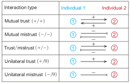
For the mixture interactions under a certain proportion of five interaction types, we construct the interaction network with individuals in the following way: i) individuals and interact with probability ; ii) the interaction strengths are categorized into five typical scenarios (see FIG. 1):
(1) Mutual trust interaction with proportion . The interaction strengths and take the values of independently.
(2) Mutual mistrust interaction with proportion . The interaction strengths and take the values of independently.
(3) Trustmistrust interaction with proportion . The interaction strengths and have opposite signs: one takes the value of while the other takes the value of .
(4) Unilateral trust interaction with proportion . One of the interaction strengths and takes the value of while the other takes the value of 0.
(5) Unilateral mistrust interaction with proportion . One of the interaction strengths and takes the value of while the other takes the value of 0.
For simplicity, we refer to the interaction network above as the complex mixture interaction network. Then, we can obtain some statistics of the interaction matrix . Specifically, we have
where
| (2) |
| (3) |
and
| (4) |
where , and .
Similar to random mixture interactions, for large , the -th row sum of matrix approaches to a constant
| (5) |
In order to clarity the -th row sum for random mixture interactions and that for complex mixture interactions, we denote them as and , respectively.
II.4 Model formulation
Consider a social network composed of individuals discussing one topic simultaneously. The opinion of individual at time is represented by . denotes the support (rejection) of individual , and represents a neutral attitude. The magnitude of indicates the strength of attitude, where represents the maximal support or rejection.
Motivated by the Altafini model proposed in [26], suppose the opinion of the -th individual evolves as
| (6) |
where
represents the weighted average influence that individual has on individual , and denotes the self-confidence level. Furthermore, let , then the system (6) can be written as
| (7) |
Remark 1
Remark 2
Definition 1
(Convergence and consensus) For large , system (7) is said to converge if , the limit exists. Moreover, it admits consensus if . If , it is said to reach the bipartite consensus, , . If it is stable.
II.5 Some basic Lemmas
Lemma 1
(See Better Theorem in [54]) Let and be an eigenpair of matrix such that satisfies the following inequalities
If digraph is strongly connected, then every Gersgorin Circle passes through .
According to Girko’s Circular law in [55] and Ellipse law in [56, 57, 58], Lemma 2 and Lemma 3 are given as below:
Lemma 2
(See Theorem 1.10 (Circular law) in [57]) Let matrix be the random matrix whose entries are i.i.d. random variables with mean zero and variance . Then, when goes to infinity, the spectral distribution of converges (both in probability and the almost sure sense) to the uniform distribution on the unit disk.
Lemma 3
(See [58]) Let matrix be the random matrix whose entries are random variables with mean zero and variance . The asymmetric entries of random matrix are i.i.d, and symmetric entries obey mean . Then, when , the spectral distribution of converges to the uniform distribution on the complex plane centered at the origin, whose horizontal half-axis length is and the vertical half-axis length is , i.e.,
Lemma 4
Consider an ellipse
then
where , . , and represent the leftmost, rightmost and uppermost points of above ellipse, respectively.
Proof 1
Substituting into the boundary equation of this ellipse, we have
and
If , then
If , then
Thus, we have
Furthermore, Substituting into the boundary equation of this ellipse, we have
and
Hence, this lemma holds.
III Problem setup
In this section, following a similar analysis to that used for the first-order continuous-time system as presented in [40, 41], we consider the convergence rate by examining the eigenvalues of matrix in system (6).
Let matrix be transformed into the “canonic” form as follows:
where each block matrix is irreducible, and and are the sets of eigenvalues of and , respectively. Moreover, . The modulus of its eigenvalues can be arranged in decreasing order
| (8) |
where denotes the -th largest modulus of eigenvalues. Especially, the eigenvalue satisfying is called the second-largest modulus eigenvalue of .
Lemma 5
Proof 2
By Lemma 1, if is an OSCC, . If is a CSCC, the distribution of eigenvalues of is divided into two cases:
1). If is structurally balanced, there exists a nonsingular matrix such that and is a nonnegative irreducible matrix. By Perron-Frobenius Theorem, and 1 is an algebraically simple eigenvalue of ;
2). If is structurally unbalanced, by Theorem 1 in [27], we have . Therefore, system (7) can achieve convergence. Moreover, if 1 is an eigenvalue of , then it is semisimple. Note that here semisimple means that the geometric and algebraic multiplicities are the same, i.e., all Jordan blocks of the eigenvalue 1 are 1 by 1.
If , it follows that can be rewritten in the following form:
where is a matrix composed of all Jordan block matrices corresponding to eigenvalue 1. and consist of all right eigenvectors and left eigenvectors corresponding to eigenvalue 1, respectively.
For one Jordan block matrix corresponding to eigenvalue , when , one obtains
It follows that the convergence rate of as is governed by . Thus, we consider as the convergence rate of .
For one Jordan block matrix corresponding to semisimple eigenvalue , when , one obtains
Then, we find that the convergence rate of depends on how quickly goes to zero. Consequently, we can generalize the convergence rate of opinions from the unsigned network, as discussed in [59], to the signed network scenario. Specifically, the convergence rate of system (7) is
From Lemma 5, according to the structural balance theory, we can identify the convergence rate of system (7) by the spectral radius or the second-largest modulus eigenvalue of . However, it remains unclear whether complex interaction types affect the convergence speed of the system. Next, we provide an example to demonstrate the significant impact that various interaction types have on the convergence rate .
Example 1
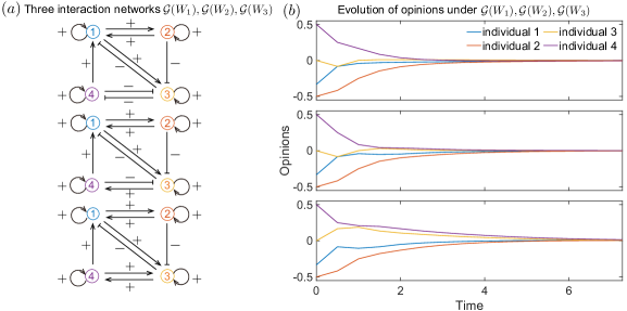
Consider the convergence rate of system (7) on three interaction networks , , , where the influence matrices corresponding to these three networks are respectively given as follows:
Note that those three networks share identical structures and edge weights in value, but the signs (interaction types) associated with edges in three networks are distinct. For instance, . Moreover, , , and . As shown in FIG. 2, complex interaction types have a significant effect on the convergence rate of the opinion dynamics model, which is often neglected in previous literature.
IV Main results
In this section, we first derive the convergence rate for random mixture interactions and further quantify the effect that some key factors have on the convergence rate, including population size , network connectivity , and self-confidence level . After that, the convergence rate of system (7) with complex mixture interactions is discussed. Finally, we present the effect of mutual interactions on convergence rate by considering two mixture scenarios and . It should be noted that the convergence rate is considered for large population size in this paper.
IV.1 Random mixture interactions
Theorem 1
The convergence rate of the system (7) with random mixture interactions is
Proof 3
For random mixture interactions, we first consider the eigenvalue distribution of matrix . Then, some statistics of matrix are given as follows:
Let , then we have
According to Lemma 2, the eigenvalues of are uniformly distributed in a unit circle centered at , as . It follows that when is sufficiently large, the eigenvalue distribution of is uniform distributed in a circle of radius approximately
Finally, note that the effect of : this shifts the circle so that it is now centered at . Then, we have
When is large, we have
i.e., By Lemma 5, the convergence rate is given as
| (9) |
Remark 3
According to Theorem 1, for random mixture interactions, it is shown that holds from an algebraic perspective, i.e., the system (7) is stable. In fact, from the viewpoint of signed graph theory, we can also analyze the reasons for stability via Theorem 1 in [27]. Based on existing results, the following equivalent results hold: all CSCCs are structurally unbalanced there is at least one negative cycle in each CSCC. When is large, the random mixture interaction network is strongly connected and there exists at least one negative cycle. In what follows, Example 2 is given to further illustrate this point.
Example 2
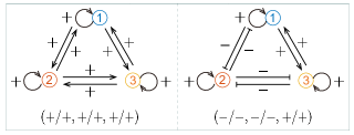
For the random mixture of different interaction types, since , when is large enough, we have , , and . Consider the probability of of the random interaction network with three individuals being structurally unbalanced.
By the definition of structural balance, the signed interaction network is structurally balanced if and only if the interaction scenario is just or (see FIG. 3). By some calculations, the probability of being structurally unbalanced is . As the population size increases, the probability that is structurally balanced tends to 1, which implies that for large .
Corollary 1
For the system (7) with random mixture interactions, the convergence rate is proportional to the population size and network connectivity, while it is inversely proportional to the individuals’ self-confidence level.
Proof 4
We prove this corollary in the following three steps:
IV.1.1 The effect of population size on convergence rate
Differentiating (9) with respect to , one obtains
where . Since for lager ,
then , i.e., larger population size improves the convergence rate of system (7).
IV.1.2 The effect of network connectivity on convergence rate
Differentiating (9) with respect to , one obtains
Since for lager ,
then , i.e., larger network connectivity leads to faster convergence of system (7).
IV.1.3 The effect of self-confidence level on convergence rate
Differentiating (9) with respect to , we obtain
Therefore, higher self-confidence level can decrease the convergence rate of system (7).
Remark 4
In most existing literature, an upper bound of the convergence rate that implicitly incorporates parameters of network properties is obtained [2, 3, 28]. However, it is difficult to directly identify the key factors that have significant impacts on the convergence rate. In contrast to previous studies, Theorem 1 provides a new perspective derived from the analysis of random matrices and explicitly establishes a specific expression for the convergence rate. Moreover, Corollary 1 quantifies the effect that some key factors have on it, thereby overcoming some limitations of existing research methods.
IV.2 Complex mixture interactions
In this subsection, we present the convergence rate of system with complex mixture interactions and study the effect of different interaction types on it. In Theorem 2, we do not consider two trivial cases, where all interaction types are mistrust or trust. Hence, we need to give the following assumption.
Assumption 1
There coexist trust and mistrust interactions in the interaction network , i.e., and .
Lemma 6
Assumption 1 holds if and only if and .
Proof 5
We prove this lemma by contradiction.
Theorem 2
Proof 6
Just as for random mixture interactions, we first consider the eigenvalue distribution of matrix . Then, we have
| (12) |
Let , then we can obtain some statistics of matrix . Specifically,
In the sequel, let , then
where . According to Lemma 3, when is sufficiently large, the eigenvalues of are uniformly distributed in an ellipse centered at (0, 0) and
It follows that the eigenvalues of are uniformly distributed in an ellipse centered at (0, 0) and
Notice is a rank-one perturbation matrix with zero eigenvalues and is a single eigenvalue. According to the low-rank perturbation theorem, when , all eigenvalues of are still uniformly distributed in the ellipse above. When eigenvalues of are still uniformly distributed in the ellipse above, whereas an eigenvalue is modified as
Since all diagonal entries , the eigenvalue distribution of is shifted leftwards along the horizontal axis. Therefore, for sufficiently large , we obtain the eigenvalue distribution of
When , the eigenvalues of are uniformly distributed in the ellipse
| (13) |
where and .
When , there is also an eigenvalue distributed outside the ellipse
| (14) |
Three endpoints , and (rightmost, leftmost, and uppermost) of the distribution in above ellipse and the unique endpoint corresponding to eigenvalue outside the ellipse (if it exists) can then be estimated as
Furthermore,
| (15) |
According to (15), for large , is sufficiently small and is bound. Moreover, and are sufficiently small. Furthermore, . Hence, . Moreover, for large , we have
In Theorem 2, we have established the quantitative expression of the convergence rate with respect to certain key factors, providing a theoretical foundation for our further analysis of how these factors influence the speed of opinion evolution. In the following subsections, we will present more specific findings in some typical scenarios, including both pure and mixed interactions, which will help us understand the role of complex interaction types in the process of opinion evolution.
IV.3 Convergence rate for five typical interaction types , and
Based on the signs of , there are five typical types of interactions, namely, mutual trust , mutual mistrust , trustmistrust , unilateral trust , unilateral mistrust . In the sequel, we will explore the convergence rate of system (7) with these five interaction types.
Assumption 2
Suppose , where is large and where
and
Remark 5
In the real world, an individual’s self-confidence level is usually not infinitely low. From a psychological perspective, it is shown that individuals’ self-confidence level usually do not drop to zero because people maintain a certain level of self-esteem and self-worth even when faced with failure. Assumption 2 implies that people maintain at least a certain level of self-confidence, which is helpful for us to facilitate our theoretical analysis in Theorem 3.
Theorem 3
Under Assumption 2, the following statements hold:
(i). For the mutual trust , trustmistrust , and unilateral trust scenarios, the convergence rate of system (7) is proportional to the population size and network connectivity, while it is inversely proportional to the individuals’ self-confidence level.
(ii). For the mutual mistrust and unilateral mistrust , the conclusions are contrary to those presented in (i).
Proof 7
(1). Mutual trust interaction.
In this case, is a row-stochastic matrix with 1 as its dominant eigenvalue, then . By Lemmas 3 and 5, the second-largest modulus eigenvalue of distributes in an ellipse (13) and determines the convergence rate. Hence, .
| (16) |
where and due to Assumption 2. Hence, increasing population size accelerates convergence. Moreover, by differentiating with respect to , we obtain
Moreover, we can obtain that stronger network connectivity promotes convergence as well.
Let
where . Then, we have
Thus, higher self-confidence level decreases convergence rate.
(2). Trustmistrust interaction.
In this case, all eigenvalues distribute in the ellipse (13), thus . Then, substituting , into (15), we have
In the sequel, we first compute and obtain
and
Next, following the similar analysis for , we consider and have
and
| (17) |
where the inequality (17) holds according to Assumption 2. In summary, we can obtain the same conclusions as in case (1).
(3). Unilateral trust interaction.
In this case, is a row-stochastic matrix with 1 as its dominant eigenvalue and thereby the second-largest modulus eigenvalue of distributed in an ellipse determines the convergence rate. By Theorem 2, . Then, substituting , into (15), we have
Similarly, we first compute and obtain
| (18) |
where
Moreover, we have
| (19) |
and
| (20) |
Then, to analyze , we have
| (21) |
Furthermore, we have
| (22) |
and
| (23) |
where the above inequality (23) holds by Assumption 2. According to (18)-(23), decreases with the increasing of and , and higher self-confidence level will decrease convergence rate.
Based on the above analysis in (1)-(3), for the , and scenarios, the convergence rate is proportional to both the population size and the network connectivity. Conversely, it is inversely proportional to the individuals’ self-confidence level.
(4). Mutual mistrust interaction.
In this case, is a row-stochastic matrix and is the dominant eigenvalue of . By Lemma 5, is an eigenvalue of and determines the convergence rate. Since , we have and Substituting them into (15), we have
| (24) |
Since , we have Moreover, .
In order to further study the effect of , and on convergence rate, differentiating (24) with respect to , and respectively, we obtain
Thus, the increase of population size and network connectivity promote the convergence rate, while the improvement of self-confidence level decreases the convergence rate.
(5). Unilateral mistrust interaction.
In this case, is a row-stochastic matrix and is the dominant eigenvalue of matrix . By Lemma 5, is an eigenvalue of and determines the convergence rate. Since , we have and Substituting them into (15), we have
Since , we have and
| (25) |
Differentiating (25) with respect to , and respectively, we obtain that the following inequalities hold
Hence, decreases with the increasing of network connectivity and population size , but increases with the higher self-confidence level .
Based on the above analysis in (4) and (5), for the and scenarios, the convergence rate is inversely proportional to both the population size and the network connectivity. On the contrary, it is proportional to the individuals’ self-confidence level.
IV.4 Mixture interaction
In this section, we focus on studying the effect of mutual trust on the convergence rate of system (7) by considering the mixture of mutual trust and mutual mistrust .
Theorem 4
For the system (7) with mixture interactions , there exist two small constants such that the following statements hold:
(i). When is in the intervals or , the convergence rate of system (7) is proportional to .
(ii). When is in the intervals or , the convergence rate of system (7) is inversely proportional to .
Proof 8
Substituting , , and into (15), we obtain
From Theorem 2, when , there exist two small constants such that . Moreover, . Thus, when , a larger can promote convergence rate , while when , conclusions are just the opposite.
Moreover, when , we have
and
where . Furthermore, since
the convergence rate monotonically decreases and increases in intervals and , respectively.
Remark 6
From Theorem 4, more trust interaction types and do not necessarily accelerate convergence. In ecology, this phenomenon is analogous to mutualism among multiple species, while in sociology, it is indicative of social balance.
IV.5 Mixture interaction
In this section, we examine the effect of increasing mutual interaction in system (7) by considering the mixture of mutual mistrust and unilateral .
Theorem 5
For the system (7) with mixture interaction , the convergence rate is inversely proportional to the proportion of mutual mistrust .
Proof 9
| (26) |
Then, differentiating (26) with respect to yields
Thus, the convergence rate is inversely proportional to the proportion of .
Remark 7
In this paper, we introduce a novel framework for analyzing the convergence rate of the discrete-time Altafini model and identify the key factors that influence this rate. Most importantly, our research method is effective not only for the discrete-time Altafini model but also for the continuous-time Altafini model as discussed in [26] and the opinion dynamics model with stubborn individuals as presented in [19].
V Illustrative examples
In this section, some numerical examples are given to illustrate our main results.
Example 3
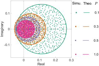
(Random mixture interactions) This example aims to show the validity of the theoretical results in Theorem 1 and Corollary 1, where the interaction strengths are drawn from a normal distribution with mean and variance .
(1). Let the parameter values be 500 and be 5, respectively. Then, by Theorem 1, we estimate the eigenvalue distribution of matrix in (7). As shown in FIG. 4, results with different parameter values from numerical simulations align well with the theoretical estimations.
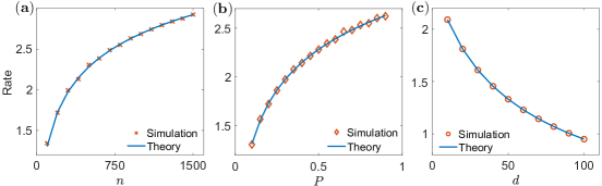
(2). Next, we verify the effects of population size, network connectivity, and individuals’ self-confidence level on the convergence rate of the system (7), where the parameter values , , and are set in TABLE 2. From Fig. 5, the results from numerical simulations are in good agreement with our theoretical analysis.
| Fig. 5 | Fig. 5 | Fig. 5 | |
| Population size | 100:100:1500 | 500 | 500 |
| Network connectivity | 0.5 | 0.1:0.05:0.9 | 0.5 |
| Self-confidence level | 5 | 5 | 10:10:100 |
Example 4
(Complex mixture interactions) This example aims to demonstrate the validity of the results on the convergence rate presented in Theorems 2 and 3. The interaction strengths are still drawn from a normal distribution with mean and variance .
(1). Set the parameter values to , , and . It is easy to verify that Assumption 2 holds. Next, by Theorems 2, we estimate the eigenvalue distribution of matrix in (7). As shown in Fig. 6, we find that the results from numerical simulations closely match the theoretical estimations.

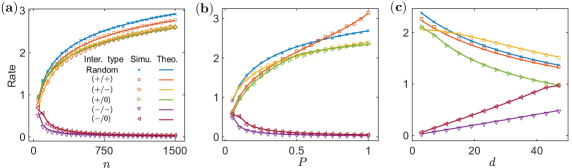
(2). Now, we verify the effects of population size, network connectivity, self-confidence level, and complex interaction types on the convergence rate of the system (7), where the parameter values , , and are provided in TABLE 3. As depicted in FIG. 7, for the , , and scenarios, an increase in population size and network connectivity results in faster convergence, whereas a higher self-confidence level slows the rate. Conversely, for the and scenarios, a higher self-confidence level accelerates convergence. Hence, these numerical simulation results are in accordance with our theoretical predictions.
| Fig. 7 | Fig. 7 | Fig. 7 | |
| Population size | 50:50:1500 | 500 | 500 |
| Network connectivity | 0.5 | 0.05:0.05:1 | 0.5 |
| Self-confidence level | 5 | 5 | 3:4:47 |
Example 5
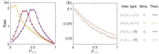
Two mixture interaction scenarios: and In this example, we focus on examining the optimal proportional configuration to ensure the fastest convergence rate for the interactions scenarios discussed in Theorems 4 and 5. Let the parameter values be , , and .
As depicted in FIG. 8, for the , , scenarios, the convergence rate is not monotonic as the proportion of the interaction type increases. Specifically, for the scenario of interaction type , when the proportion of is approximately 0.5 , system (7) achieves convergence in the fastest speed. From FIG. 8 , for the scenario, the convergence rate is inversely proportional to the proportion of interaction types.
VI Conclusion
A general framework for the analysis of the convergence rate is established in this paper. Firstly, we have established the quantitative expressions of convergence rate by random matrix theory and low-rank perturbation theory. These results bridge the gap between the convergence rate and complex interaction types. With the aid of this bridge, we have further analyzed the impact of some key factors on the convergence rate through rigorous theoretical derivations. In addition to theoretical analyses, we have also provided simulation examples to corroborate our findings, thereby demonstrating the significant impact of interaction types on the convergence rate.
In a realistic social network, the information transmitted among the individuals may be subject to communication constraints such as delays from time to time, ranging from engineering science (distributed control [60, 61]) to ecosystems (ecological stability [62]), and social sciences (opinion forming [63]). From the perspective of opinion dynamics, a communication delay between a pair of individuals represents that one individual can only access an earlier opinion of the other, which leads to the fact that individuals cannot express their opinions in a precise manner. This naturally raises a significant question: what impact does time delay have on the convergence rate of opinion dynamics? Whether our approach in this paper can be extended to such a situation remains open for future investigations.
References
References
- [1] M. Cao, A. Morse, and B. Anderson, Reaching a consensus in a dynamically changing environment: Convergence rates, measurement delays, and asynchronous event, SIAM J. Control Optim. 47, 601 (2008).
- [2] A. Olshevsky, and J. N. Tsitsiklis, Convergence speed in distributed consensus and averaging, SIAM Review 53, 747 (2011).
- [3] J. Xu, H. Zhang, and L. Xie, Stochastic approximation approach for consensus and convergence rate analysis of multiagent systems, IEEE Trans. Autom. Control 57, 3163 (2012).
- [4] M. Angulo and J. Slotine, Qualitative stability of nonlinear networked systems, IEEE Trans. Autom. Control 62, 4080 (2017).
- [5] Z. Ji, H. Lin, and H. Yu, Protocols design and uncontrollable topologies construction for multi-agent networks,” IEEE Trans. Autom. Control 60, 781 (2015).
- [6] Y. Hong, G. Chen, and L. Bushnell, Distributed observers design for leader-following control of multi-agent networks, Automatica 44, 846 (2008).
- [7] W. Li and G. Chen, The designated convergence rate problem of consensus or flocking of double-integrator agents with general non-equal velocity and position couplings, IEEE Trans. Autom. Control 62, 412 (2017).
- [8] C. W. Reynolds, Flocks, herds, and schools: A distributed behavioral model, Comput. Graph 25 (1987).
- [9] T. Vicsek, A. Czirók, E. Ben-Jacob, I. Cohen, and O. Shochet, Novel type of phase transition in a system of self-driven particles, Phys. Rev. Lett. 75, 1226 (1995).
- [10] A. V. Proskurnikov and R. Tempo, A tutorial on modeling and analysis of dynamic social networks. Part I, Annu. Rev. Control 43, 65 (2017).
- [11] A. V. Proskurnikov and R. Tempo, A tutorial on modeling and analysis of dynamic social networks. Part II, Annu. Rev. Control 45, 166 (2018).
- [12] W. Xia, M. Ye, J. Liu, M. Cao, and X. Sun, Analysis of a nonlinear opinion dynamics model with biased assimilation, Automatica 120, 109113 (2020).
- [13] L. Wang, Y. Hong, G. Shi, and C. Altafini, Signed social networks with biased assimilation, IEEE Trans. Autom. Control 67, 5134 (2022).
- [14] M. H. DeGroot, Reaching a consensus, J. Amer. Stat. Assoc. 69, 118 (1974).
- [15] N. E. Friedkin and E. C. Johnsen, Social influence networks and opinion change, Adv. Group Process 16, 1 (1999).
- [16] C. Altafini and F. Ceragioli, Signed bounded confidence models for opinion dynamics, Automatica 93, 114 (2018).
- [17] Y. Tian, and L. Wang, Opinion dynamics in social networks with stubborn agents: An issue-based perspective, Automatica 96, 213 (2018).
- [18] L. Wang, Y. Tian, and J, Du, Opinion dynamics in social networks, Scientia Sinca Informations 48, 3 (2018).
- [19] N. E. Friedkin, A. V. Proskurnikov, R. Tempo, and S. E. Parsegov, Network science on belief system dynamics under logic constraints, Science 354, 321 (2016).
- [20] H. Yang, J. Cao, Y. Yuan, and J. Wang, Modulus consensus for time-varying heterogeneous opinion dynamics on multiple interdependent topics, IEEE Trans. Autom. Control 68, 6913 (2023).
- [21] G. Chen, X. Duan, N. E. Friedkin, and F. Bullo, Social power dynamics over switching and stochastic influence networks, IEEE Trans. Autom. Control 64, 582 (2019).
- [22] Y. Tian, P. Jia, A. MirTabatabaei, L. Wang, N. E. Friedkin, and F. Bullo, Social power evolution in influence networks with stubborn individuals, IEEE Trans. Autom. Control 67, 574 (2022).
- [23] M. Ye, Y. Qin, A. Govaert, B. D. O. Anderson, and M. Cao, An influence network model to study discrepancies in expressed and private opinions, Automatica 107, 371 (2019).
- [24] Q. Liu, L. Chai, and M. Li, Dynamics of expressed and private opinion evolution over issue sequences, IEEE Trans. Comput. Soc. Syst. 10, 2860 (2023).
- [25] D. Cartwright and F. Harary, Structural balance: A generalization of Heider’s theory, Psychol. Rev. 63, 277 (1956).
- [26] C. Altafini, Consensus problems on networks with antagonistic interactions, IEEE Trans. Autom. Control 58, 935 (2013).
- [27] W. Xia, M. Cao, and K. H. Johansson, Structural balance and opinion separation in trust-mistrust social networks, IEEE Trans. Control Netw. Syst. 3, 46 (2016).
- [28] J. Liu, X. Chen, T. Tamer Başar, and M. A. Belabbas, Exponential convergence of the discrete- and continuous-time Altafini models, IEEE Trans. Autom. Control 62, 6168 (2017).
- [29] V. Amelkin, F. Bullo, and A. K. Singh, Polar opinion dynamics in social networks, IEEE Trans. Autom. Control 62, 5650 (2017).
- [30] P. Cisneros-Velarde, K. S. Chan, and F. Bullo, Polarization and fluctuations in signed social networks, IEEE Trans. Autom. Control 66, 3789 (2021).
- [31] D. Meng, M. Du, and Y. Jia, Interval bipartite consensus of networked agents associated with signed digraphs, IEEE Trans. Autom. Control. 61, 3755 (2016).
- [32] D. Meng, Convergence analysis of directed signed networks via an M-matrix approach, Int. J. Control 91, 827 (2017).
- [33] A. V. Proskurnikov, A. Matveev, and M. Cao, Opinion dynamics in social networks with hostile camps: Consensus vs. polarization, IEEE Trans. Autom. Control 61, 1524 (2016).
- [34] L. Shi, W. Li, M. Shi, K. Shi, and Y. Cheng, Opinion polarization over signed social networks with quasi-structural balance, IEEE Trans. Autom. Control 68, 6867 (2023).
- [35] F. Liu, D. Xue, S. Hirche, and M. Buss, Polarizability, consensusability, and neutralizability of opinion dynamics on coopetitive networks, IEEE Trans. Autom. Control 64, 3339 (2019).
- [36] F. Liu, S. Cui, W. Mei, F. Dörfler, and M. Buss, Interplay between homophily-based appraisal dynamics and influence-based opinion dynamics: modeling and analysis, IEEE Control Syst. Lett. 5, 181 (2021).
- [37] Z. Ding, X. Chen, Y. Dong, S. Yu, and F. Herrera, Consensus convergence speed in social network DeGroot model: The effects of the agents with high self-confidence levels, IEEE Trans. Comput. Soc. Syst. 10, 2882 (2023).
- [38] J. Ghaderi and R. Srikant, Opinion dynamics in social networks with stubborn agents: Equilibrium and convergence rate, Automatica 50, 3209 (2014).
- [39] A. Nedić, A. Olshevsky, and C. A. Uribe, Graph-theoretic analysis of belief system dynamics under logic constraints, Scientific Rep. 9, 8843 (2019).
- [40] R. Olfati-Saber and R. M. Murray, Consensus problems in networks of agents with switching topology and time-delays, IEEE Trans. Autom. Control 49, 1520 (2004).
- [41] W. Yu, G. Chen, M. Cao, and J. Kurths, Second-order consensus for multiagent systems with directed topologies and nonlinear dynamics, IEEE Trans. Syst., Man, Cybern. Part B 40, 881 (2010).
- [42] L. Xiao and S. Boyd, Fast linear iterations for distributed averaging, Syst. Control Lett. 53, 65 (2004).
- [43] S. Apers and A. Sarlette, Accelerating consensus by spectral clustering and polynomial filters, IEEE Trans. Control Netw. Syst. 4, 544 (2017).
- [44] H. Zhang, Z. Chen, and X. Mo, Effect of adding edges to consensus networks with directed acyclic graphs, IEEE Trans. Autom. Control 62, 4891 (2017).
- [45] L. Wang and F. Xiao, Finite-time consensus problems for networks of dynamic agents, IEEE Trans. Autom. Control 55, 950 (2010).
- [46] F. Xiao, L. Wang, and T. Chen, Finite-time consensus in networks of integrator-like dynamic agents with directional link failure, IEEE Trans. Autom. Control 59, 756 (2014).
- [47] J. Yi, L. Chai, and J. Zhang, Average consensus by graph filtering: new approach, explicit convergence rate, and optimal design, IEEE Trans. Autom. Control 65, 191 (2020).
- [48] J. Qin, H. Gao, and C. Yu, On discrete-time convergence for general linear multi-agent systems under dynamic topology, IEEE Trans. Autom. Control 59, 1054 (2014).
- [49] Q. Ma, J. Qin, B. D. O. Anderson, and L. Wang, Exponential consensus of multiple agents over dynamic network topology: controllability, connectivity, and compactness, IEEE Trans. Autom. Control 68, 7104 (2023).
- [50] S. Mariano, I. C. Morarescu, R. Postoyan, and L. Zaccarian, A hybrid model of opinion dynamics with memory-based connectivity, IEEE Control Syst. Lett. 4, 644 (2020).
- [51] J. Yi, L. Chai, and J. Zhang, Convergence rate of accelerated average consensus with local node memory: optimization and analytic solutions, IEEE Trans. Autom. Control 68, 7254 (2023).
- [52] H. Zhang and Z. Chen, Consensus acceleration in a class of predictive networks, IEEE Trans. Neural Netw. Learn. Syst. 25, 1921 (2014).
- [53] T. Wang, H. Zhang, and Y. Zhao, Consensus of multi-agent systems under binary-valued measurements and recursive projection algorithm, IEEE Trans. Autom. Control 65, 2678 (2020).
- [54] R. A. Horn and C. R. Johnson, Matrix Analysis, (Cambridge University Press, Cambridge UK, 2012).
- [55] V. L. Girko, “Circular law, Theory Probab. Appl. 29, 694 (1985).
- [56] H. J. Sommers, A. Crisanti, H. Sompolinsky, and Y. Stein, Spectrum of large random asymmetric matrices, Phys. Rev. Lett. 60, 1895 (1988).
- [57] T. Tao, V. Vu, and M. Krishnapur, Random matrices: Universality of ESDs and the circular law, Ann. Probab. 38, 2023 (2010).
- [58] S. Allesina and S. Tang, Stability criteria for complex ecosystems, Nature 483, 205 (2012).
- [59] E. Seneta, Non-negative Matrices and Markov Chains, (New York: Springer, 2006).
- [60] C. K. Zhang, Y. He, L. Jiang, M. Wu, and H. -B. Zeng, Delay-variation-dependent stability of delayed discrete-time systems, IEEE Trans. Autom. Control 61, 2663 (2016).
- [61] C. K. Zhang, Y. He, L. Jiang, and M. Wu, Notes on stability of time-delay systems: bounding inequalities and augmented lyapunov-krasovskii functionals, IEEE Trans. Autom. Control 62, 5331 (2017).
- [62] Y. Yang, K. R. Foster, K. Z. Coyte, and A. Li, Time delays modulate the stability of complex ecosystems, Nat. Ecol. Evol. 7, 1610 (2023).
- [63] Y. Zou, W. Wang, K. Xia, and Z. Zuo, Convergence of opinion dynamics with heterogeneous asymmetric saturation levels and time-varying delays, IEEE Trans. Netw. Sci. Eng. 11, 3189 (2024).