Structural causal influence (SCI) captures the forces of social inequality in models of disease dynamics

Abstract

Mathematical modelling has served a central role in studying how infectious disease transmission manifests at the population level. These models have demonstrated the importance of key population-level factors like social network heterogeneity on structuring epidemic risk and are now routinely used in public health and healthcare for decision support. One barrier to broader utility of mathematical models in epidemiology is that the existing canon does not readily accommodate the social determinants of health as distinct, formal drivers of variability in transmission dynamics. Given the decades of empirical support for the organizational effect of social determinants on health burden more generally and infectious disease risk more specially, addressing this modelling gap is of critical importance. In this study, we build on prior efforts to meaningfully integrate social forces into mathematical epidemiology by introducing several new metrics, principally . Here, leverages causal analysis to provide a measure of the relative vulnerability of subgroups within a susceptible population, which are crafted by differences in healthcare access, exposure to disease, and other determinants driven by social forces. We develop our metrics using a general case and apply it to specific one of public health importance: Hepatitis C virus (HCV) in a population of persons who inject drugs (PWID). Our use of the SCI reveals that, under specific parameters in a multi-community disease model, the “less vulnerable” (better-resourced) community may sustain a basic reproduction number below one when isolated, ensuring disease extinction. However, even minimal transmission between less and more vulnerable communities can elevate this number, potentially leading to sustained epidemics within (and across) both communities. Summarizing, we reflect on our findings in light of the modern conversation surrounding the importance of social inequalities and how their consideration can influence the study and practice of mathematical epidemiology.

Author summary

Since its inception, the field of public health has embraced the study of the social determinants of health, which focuses on how socially-mediated forces can render certain communities more vulnerable to negative health outcomes. More recently, epidemiologists have sought to integrate social determinants into their models of epidemics. However, our ability to distinguish the effects of social determinants from other factors remains a challenge. In this study, we introduce several new mathematical metrics that allow us to more carefully understand how social forces—unequal access to care, segregation, and others—craft disparate outcomes. We focus on the ”structural causal influence,” a measure of the vulnerability of certain communities to outbreaks relative to others in a setting where social determinants are at work. In doing so, we hope to modernize mathematical epidemiology by equipping it with tools to better capture how widespread social inequalities shape epidemics around the world.

1 Introduction

In the last several decades, scholars of various kinds have questioned many of the classical assumptions of computational epidemiology [1, 2]. Encouragingly, many of these criticisms have been crystallized into new modeling frameworks (e.g., network-based and stochastic simulation styles) that aim to capture better features of the natural world [3, 4, 5, 6]. This includes an appreciation for differences in pathogen biology and host behavior, and their role in phenomena like complex contagion [7, 8, 9], the role of crowding [10], adaptive behavior [11], and superspreading [12]. These constitute just a sample of the features that are adding richness to epidemiological models.

Interest in the “social determinants of health (SDOH)” has grown enormously over the past several decades. The World Health Organization defines them as “the non-medical factors that influence health outcomes,” i.e., the “conditions in which people are born, grow, work, live, and age, and the broader set of forces and systems shaping the conditions of daily life” [13]. Scholars of SDOH have created a new vocabulary for the study of diseases by emphasizing the forces that craft unique experiences for different populations. It has been animated in related phenomena, such as the “health disparities” movement in the United States, which highlights how forces such as discrimination lead to disproportionate health burden [14, 15], even influencing the evolutionary and ecological features of disease [16, 15]. Both are seen as manifestations of structural and social inequalities.

Over a century of study in epidemiology has demonstrated a strong association between health outcomes and socioeconomic status [17]. And yet, the social determinants of health are rarely formalized in mathematical epidemiology. The title of an influential 2020 article by Melanie Moses and Kathryn Powers succinctly stated: “Well-mixed models do not protect the vulnerable in segregated societies [18].” That is, the assumptions of disease modeling often inadequately address how disease burden manifests in unequal societies . There are, however, examples of studies that have used mathematical modeling to examine phenomena where inequalities manifest, such as the spread of HIV and HCV in persons who inject drugs [19, 20, 21] or with regards to infectious spread in prisons [22]. More recently, scholars have offered syntheses that have remarked on the need to color mathematical modeling with social forces [23, 24, 25, 26], or commented on how targeting poor populations can lead to better outcomes in tuberculosis [27]. However, these studies have not transformed the standard language of mathematical epidemiology.

Here, we reconcile classical formulations in mathematical epidemiology with an understanding of the powerful role of social inequalities in crafting the shape of epidemics. We develop mathematical models that consider the experience of different subpopulations that compose a larger susceptible population. We analyze them using standard mathematical methods and develop metrics that add depth to epidemiological models by highlighting how SDOH influence disease dynamics. In addition to introducing two variations on classical metrics—the relative basic reproductive number (RRN, $\mathcal{A}$) and the relative force of infection (R-FoI, $\mathcal{F}_{i}$)—we propose the (SCI, $\mathcal{C}_{i}$) as a robust measure of how inequalities can affect disease dynamics. We utilize a causal inference framework using the “pearls of philosophy” definition of causation [28]. The primary goal is to understand the variables associated with cause and effect (the measure of one variable’s impact on the measure of another variable). The broader, fundamental question is: how is event [X] affected by another event [Y]? We use the idea of structural causation to ask the more specific question: “How do social inequalities affect disease dynamics?”

We discuss the benefits of SCI as a new means through which we can understand systems where subpopulations are affected by contagion in different ways and reflect on it in terms of contemporary issues in public health. In doing so, we offer methods for how we can model and, more broadly, study contemporary epidemics with a heightened sensitivity to the centrality of social forces in dictating the pace and direction of infectious outbreaks. Summarizing, we discuss the implications of our metrics for broader efforts to integrate social determinants into both the technical realms and public sphere, and propose ways that the SCI and other metrics can be applied in other outbreak scenarios.

All major symbols used throughout the article are listed in Table 1.

Table 1: For clarity, we provide a list of symbols used throughout the article to denote relevant quantities and functions.

Symbol	Description

2 Methods

To introduce the basics of our approach and establish a common vocabulary (legible to anyone who studies mathematical or computational epidemiology), we will utilize the canonical Susceptible-Infectious-Recovered (SIR) model [29]. In these models, host populations are divided into different compartments, where homogeneity is assumed among individuals within the same compartment, and the movement of individuals between compartments is parameterized by a system of . While extremely useful for helping epidemiologists analyze overall infectious disease dynamics, the underlying assumptions of parameter value distributions and homogeneity in the population often need to be more representative of reality. In particular, one can consider how health inequalities can shape parameter values [30, 31]:

• Differences in exposure
  Examples: Crowding in households [32, 33], medical facilities, public transportation, and/or occupational factors such as the inability to work from home [34] or dependence on childcare outside of the home [35].

• Differences in susceptibility
  Examples: Host factors, such as pre-existing immunity, age, other underlying diseases or conditions [36], smoking and/or environmental tobacco smoke [37], nutritional status [38, 39], stress, and/or vaccination status, where there may be differences in vaccine acceptance, uptake and/or access [40].

• Differences in timely effective treatment
  Examples: Access to outpatient and inpatient medical care [41], care-seeking attitudes and behavior [42], financial obstacles (including lack of adequate insurance coverage) [43], and logistical obstacles, such as transportation, language [44], quality of care, and/or availability of treatments.

Within compartmental models, variations in susceptibility and exposure are anticipated to impact the transmission rate, while distinctions in timely and effective treatment may influence the mean infectious period. Therefore, we demonstrate how the study of the influence of “social determinants of health (SDOH)” on infectious disease dynamics can be formally integrated into mathematical epidemiology by constructing a compartmental model (Figure 1). One of the challenges in modeling is that distinct model structures can produce similar dynamics [45, 46]. This phenomenon is referred to as the identifiability problem. In the context of SDOH, this implies that one can construct a model that accurately captures the dynamics of a disease system while overlooking the influence of SDOH. Consequently, prevalent model structures, such as the basic SIR model, might yield accurate dynamics despite incorporating incorrect parameters or variables. An analytical demonstration of this issue can be found in the supplementary document (Section A.1.1).

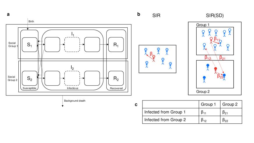
Figure 1: (a) Schematic for a general epidemiological compartmental model with two social groups. (b) Using the SIR model as an example, this schematic depicts the average transmission rate(s) between infected (red) and susceptible (blue) individuals in the SIR model and the SIR model considering social determinants (SIR(SD) model). In the SIR(SD) model, group 1 individuals (depicted as unshaded) are more vulnerable and have higher effective contact rates compared to group 2 individuals (filled in). (c) Table summarizing the transmission rates/effective contact rates, $\beta_{ij}$, from an infected individual in group i to group j, for the example SIR(SD) model shown in (b).

The primary objective of this study is to assess the impact of SDOH on epidemiological parameters by employing compartmental models. This section introduces metrics designed to analyze the influence of SDOH on disease dynamics. We develop three such metrics, with a detailed examination of one within the confines of this article. We aim to elucidate the ramifications of social inequalities on disease dynamics and measure the impact of social determinants. To facilitate a thorough and meticulous exploration, we delve into the Susceptible-Infected-Recovered (SIR) epidemiological model incorporating social determinants, and then use the dynamics of the Hepatitis C virus as a specific case study. In doing so, we demonstrate to readers that they can readily apply these metrics to various general compartmental epidemiological models.

Note: We use the terms “group” and “community” interchangeably throughout the manuscript, opting for “community” often when talking about the real-world example of a Hepatitis C virus outbreak in a population of persons who inject drugs (PWID). In addition, we frequently discuss “group 1” and “group 2” as our subpopulations, since our models consider the specific scenario where there are two distinct social subpopulations.

2.1 Measuring the influence of the social determinants of health (SDOH) in infectious diseases

Here, we introduce a new metric, the “ of a social group ($\mathcal{C}_{i}$),” derived through causal inference to quantify the impact of SDOH on infectious disease epidemiological dynamics. We will apply this metric using our SIR(SD) model. Additionally, we will apply this metric to our HCV(SD) model, developed to describe the dynamics of a outbreak in a population defined by two small social groups. Furthermore, we introduce two new metrics derived from the traditional approach of basic reproduction number and force of infection, which can also be used to quantify the influence of SDOH on infectious disease epidemiological dynamics: , () and the of a social group (). In the scope of this article, we will discuss some aspects of these measures using our SIR(SD) model. We summarize all these new measures in Table 3 and describe how they can be calculated for our SIR(SD) model. These measures are detailed in the following subsections.

2.1.1 Structural causal influence of social group $i$, $\mathcal{C}_{i}$

Structural causal models, as introduced in [28, 47], can be utilized to measure the effect of each social group on disease dynamics. Here, we use a deterministic version of structural causal models for as discussed in [48]. Interventions in the compartmental disease models with SDOH can be modified differently. We utilize perfect interventions [48] since our goal is to determine the “individual” influence of each social group on the overall dynamics of the system. In the context of the SIR(SD) model, perfect interventions mean that we will set the value of the infectious population of the considered group to be zero and assume that the intervention is activated from time $t=0$ to $t\rightarrow\infty$. This means that the considered infectious population is absent and remains unchanged over time. We follow the notion described in [48], inspired by the do-operator introduced by [28]. We will denote this type of intervention as $\text{do}(\Gamma)$, where $\Gamma$ represents the conditions required for “perfect” interventions. Using the change in $\mathcal{R}_{0}$ due to SDOH, the of social group $i$ on disease dynamics can be defined as follows:

$$\mathcal{C}_{i}=\frac{\mathcal{R}_{0}^{\text{SD}}-\mathcal{R}_{0}^{\text{do}(\Gamma_{i})}}{\mathcal{R}_{0}^{\text{SD}}},$$ (1)

where $\mathcal{R}_{0}^{\text{SD}}$ is the basic reproduction number for the compartmental model incorporating SDOH, and $\mathcal{R}_{0}^{\text{do}(\Gamma_{i})}$ denotes the basic reproduction number for the same model with intervention for group $i$. For any general epidemiological model, the computational steps presented in Section 2.1.1 can be used to calculate the .

Notes on SCI, $\boldsymbol{\mathcal{C}_{i}}$

Our metric, called the , offers a comparative analysis of disease dynamics within the full model, encompassing multiple social groups, and a model representing the effects of perfect interventions within one specific group. It quantifies the disparity in secondary infections between the total population and the population under perfect interventions for the designated social group. To standardize this measure, it is normalized by the total secondary infections within the population, resulting in a scale ranging from 0 to 1. A value closer to zero suggests a convergence between the dynamics of the full model and the perfect intervention model for the specified group. In such cases, the influence of the considered group is relatively minimal, indicating an inability to halt disease transmission solely within that group. Conversely, a higher SCI value signifies significant discrepancies between the dynamics of the full model and the perfect intervention model, highlighting a substantial influence exerted by that particular group. Specific features of the SCI can be summarized as follows:

• The SCI value $\mathcal{C}_{j}$ for a given social group $j$ lies within the range $0\leq\mathcal{C}_{j}\leq 1$, where $\mathcal{C}_{j}$ measures the influence of group $j$ on disease dynamics.

• In scenarios with only two social groups $j$ and $l$, the basic reproduction number for perfect interventions within group $j$ aligns with the basic reproduction number for an isolated group $l$, devoid of inter-group contacts.

• For two social groups $j$ and $l$, the SCI value of $\mathcal{C}_{j}=0$ indicates that group $l$ exhibits the highest basic reproduction number in the absence of inter-group contacts.

• In the context of two social groups $j$ and $l$, the SCI value of $\mathcal{C}_{j}=1$ signifies that group $l$ experiences no secondary infections in the absence of inter-group contacts.

2.1.2 Relative Reproduction Number, $\mathcal{A}$

The relative reproductive number, denoted as $\mathcal{A}$, provides a metric to evaluate how SDOH influences epidemiological dynamics. It quantifies the extent to which SDOH shapes these dynamics relative to a baseline scenario. Mathematically, $\mathcal{A}$ is defined as:

$$\mathcal{A}=\frac{\mathcal{R}_{0}^{\text{SD}}}{\mathcal{R}_{0}},$$ (2)

where $\mathcal{R}_{0}^{\text{SD}}$ represents the basic reproduction number for the compartmental model incorporating SDOH, while $\mathcal{R}_{0}$ signifies the basic reproduction number for the equivalent compartmental model that does not consider SDOH. In scenarios where $\mathcal{R}_{0}<1$ and $\mathcal{A}>1$, it is conceivable to encounter a situation where the basic model suggests that the disease cannot establish an epidemic in the population. However, the inclusion of SDOH in the model could indicate that the disease has the potential to invade the population if $\mathcal{R}_{0}^{\text{(SD)}}=\mathcal{A}\mathcal{R}_{0}>1$.

2.1.3 Relative force of infection (FoI) of social group $i$, $\mathcal{F}_{i}$

The force of infection is defined as “the rate at which susceptible individuals in a population acquire an infectious disease in that population, per unit time.“ It is also known as the incidence rate or hazard rate [49, 50]:

$$\lambda=\frac{c_{e}I_{t}}{N_{t}},$$ (3)

where $\lambda$ is the force of infection at time $t$, $c_{e}$ is the number of individuals effectively contacted by each person per unit time, $I_{t}$ is the number of infected individuals in the population at time $t$, and $N_{t}$ is the total population size at time $t$.

Here, we define the relative FoI for different groups as follows:

$$\mathcal{F}_{i}=\frac{\lambda_{i}^{\text{SD}}}{\lambda^{\text{SD}}},\textit{ for }i=1,\ 2,$$ (4)

where $\lambda^{\text{SD}}=\lambda_{1}^{\text{SD}}+\lambda_{2}^{\text{SD}}$ and $\lambda_{i}^{\text{SD}}$ represent the FoI for group $i=1,\ 2$ under the compartmental model incorporating SDOH.

3 Results

We will first present a roadmap for the results section, outlining how we will present our findings:

• Having introduced metrics for quantifying the influence of the “social determinants of health (SDOH)” on infectious disease epidemiological dynamics (Section 2.1), we explore how they can be utilized in epidemiological models.

• We start with a general SIR(SD) model and explore how these metrics can be applied to different transmission/mixing scenarios (see Section 3.1).

• We then extend our analysis to a compartmental model specific to , where we consider the role of additional parameters, etc. (see Section 3.2).

• Appendix A has other important supplementary information: further exploring the relationship between parameters in the SIR vs. SIR(SD) models (Section A.1), the identifiability problem (Section A.1.1), and additional analyses, including how they support the arguments in the main text (Section A.2–Section A.4).

3.1 SIR(SD) model

In the SIR(SD) model, we consider two social groups and partition each social group into three compartments: susceptible (S), infectious (I), and recovered (R), as shown in Figure 1(a). In other words, the structure follows a standard SIR model, where each compartment has been broken down into two sub-compartments representing a different social group. The following system of describes the model:

$$\frac{dS_{1}}{dt} =-(\beta_{11}I_{1}+\beta_{12}I_{2})\frac{S_{1}}{N_{1}}$$ (5)

$$\frac{dS_{2}}{dt} =-(\beta_{21}I_{1}+\beta_{22}I_{2})\frac{S_{2}}{N_{2}}$$

$$\frac{dI_{1}}{dt} =(\beta_{11}I_{1}+\beta_{12}I_{2})\frac{S_{1}}{N_{1}}-\gamma_{1}I_{1}$$

$$\frac{dI_{2}}{dt} =(\beta_{21}I_{1}+\beta_{22}I_{2})\frac{S_{2}}{N_{2}}-\gamma_{2}I_{2}$$

$$\frac{dR_{1}}{dt} =\gamma_{1}I_{1}$$

$$\frac{dR_{2}}{dt} =\gamma_{2}I_{2}$$

where $S_{i}+I_{i}+R_{i}=N_{i}$ for $i=1,2$, and $N_{1}+N_{2}=N$, where $N$ denotes the total population. We assume that $N,N_{1},N_{2}$ remain constant over time and that the variables $S_{i}$, $I_{i}$, and $R_{i}$ are constrained to satisfy $0\leq S_{i},I_{i},R_{i}\leq N_{i}$. For comparison between the basic SIR model and our SIR(SD) model, we will consider the relationships: $S=S_{1}+S_{2}$, $I=I_{1}+I_{2}$, and $R=R_{1}+R_{2}$.

3.1.1 Parameters in the SIR vs. SIR(SD) models

In the standard SIR model, $\beta$ represents the transmission rate (or effective contacts per unit period) and $\frac{1}{\gamma}$ signifies the mean infectious period, and both parameters are assumed to remain constant. In the case of the mean infectious period, this assumption can equivalently be stated as the distribution of the infectious period being exponential with a mean value of $\frac{1}{\gamma}$[51, 52]. It is worth noting that this corresponds to a specific case of the Gamma distribution, specifically the $\text{Gamma}(1,\gamma)$ distribution.

In the SIR(SD) model, we have employed the same notation to represent the parameters for transmission rates and mean infectious periods for both social groups. However, to account for the limitation of assuming homogeneity in the population, including in mixing patterns [53, 54, 55], we incorporate different averages of interactions within and between groups to give rise to four distinct transmission rates, as illustrated in Figure 1(b) and (c). Similarly, we account for differences in recovery by assuming that the infectious period for each group follows a Gamma distribution with means of $\frac{1}{\gamma_{1}}$ and $\frac{1}{\gamma_{2}}$ for social groups 1 and 2, respectively.

The unique parameters in the SIR(SD) model can be expressed in terms of the population-level parameters used in the standard SIR model. Here, we summarize the relationship between the parameters of both models by describing the parameters of the SIR(SD) model in terms of the population-wide SIR model parameters and a set of control parameters, as shown in Table 2. The parameters $w_{0},w_{1},w_{2}$ regulate the values of the SIR(SD) transmission parameters, $\beta_{ij}$ with respect to $\beta$ (SIR model), and the parameter, $a$, regulates the values of the SIR(SD) mean infectious periods, $\frac{1}{\gamma_{i}}$ with respect to $\frac{1}{\gamma}$ (SIR model). Further details regarding the comparison between the parameters of the SIR and SIR(SD) models are provided in the supplemental information (see Section A.1).

Group level parameter	Relationship with population-level parameter ($\beta$ or $\gamma$)
$\beta_{11}$	$\beta(1+w_{0})w_{1}$
$\beta_{21}$	$\beta(1+w_{0})(1-w_{1})$
$\beta_{22}$	$\beta(1-w_{0})w_{2}$
$\beta_{12}$	$\beta(1-w_{0})(1-w_{2})$
$\frac{1}{\gamma_{1}}$	$\frac{1+a}{2\gamma}\frac{N}{N_{1}}$
$\frac{1}{\gamma_{2}}$	$\frac{1-a}{2\gamma}\frac{N}{N_{2}}$

Table 2: Relationship Between Group-Level parameters ($\beta_{ij}$, $\frac{1}{\gamma_{i}}$ for transmission and mean infectious periods respectively) and Combined Population Transmission Rate ($\beta$, $\frac{1}{\gamma}$). For transmission rates, the parameter $w_{0}$ can take values in the interval $[-1,1]$, while the parameters $w_{1}$ and $w_{2}$ are within the closed unit interval. For the mean infectious period, the parameter $a$ adheres to the following constraint: $-1<\frac{N_{1}-N_{2}}{N}<a<1$.

3.1.2 $\mathcal{R}_{0}$ and measures for quantifying the influence of SDOH in the SIR(SD) model

The basic reproduction number, $\mathcal{R}_{0}$, measures the average number of secondary infections caused by an infectious individual in a susceptible population [56, 57]. In infectious disease epidemiology, it is primarily used to predict if a disease outbreak will persist or die out. Here, we derive the $\mathcal{R}_{0}$ for the SIR(SD) model, henceforth referred to as $\mathcal{R}_{0}^{\text{SIR(SD)}}$.

The disease-free equilibrium of this model is given by $(S_{1}^{*},S_{2}^{*},I_{1}^{*},I_{2}^{*},R_{1}^{*},R_{2}^{*})=(N_{1},N_{2},0,0,0,0)$. Using the next-generation matrix method [58, 57], we derive $\mathcal{R}_{0}^{\text{SIR(SD)}}$:

$$\mathcal{R}_{0}^{\text{SIR(SD)}}=\frac{1}{2}\left(\left(\frac{\beta_{11}}{\gamma_{1}}+\frac{\beta_{22}}{\gamma_{2}}\right)+\sqrt{\left(\frac{\beta_{11}}{\gamma_{1}}-\frac{\beta_{22}}{\gamma_{2}}\right)^{2}+\frac{4\beta_{12}\beta_{21}}{\gamma_{1}\gamma_{2}}}\ \right).$$ (6)

Hence, the disease-free equilibrium is stable when the basic reproduction number $\mathcal{R}_{0}^{\text{SIR(SD)}}<1$, indicating that the disease cannot invade the population. Conversely, it becomes unstable if $\mathcal{R}_{0}^{\text{SIR(SD)}}>1$, signifying that an invasion is always possible [57, 59, 60].

The relative reproduction number, $\mathcal{A}$, is logically dependent on the impact of SDOH on disease dynamics, which in the SIR(SD) model, are represented by the control parameters $w_{0}$, $w_{1}$, $w_{2}$, and $a$, as well as the population sizes of each group ($N_{1}$ and $N_{2}$) and total population ($N$). Hence, the value of $\mathcal{A}$ in the SIR(SD) can be expressed as:

$$\mathcal{A}=\frac{N}{4}\left(\left(\mathcal{A}_{1}w_{1}+\mathcal{A}_{2}w_{2}\right)+\sqrt{\left(\mathcal{A}_{1}w_{1}+\mathcal{A}_{2}w_{2}\right)^{2}+4\mathcal{A}_{1}\mathcal{A}_{2}(1-w_{1}-w_{2})}\leavevmode\nobreak\ \right),$$ (7)

where $\mathcal{A}_{i}=\frac{(1+(-1)^{i-1}w_{0})(1+(-1)^{i-1}a)}{N_{i}}\leavevmode\nobreak\$ for $i=1,\ 2$. Similarly, the computations for and relative force of infection can be performed, and the final expressions for these values are summarized in Table 3.

Metric	General Formula	Formula for SIR(SD) model
$\mathcal{A}$	$\mathcal{R}_{0}^{\text{SD}}/\mathcal{R}_{0}$	$\frac{N}{4}\left(\left(\mathcal{A}_{1}w_{1}+\mathcal{A}_{2}w_{2}\right)+\sqrt{\Delta}\leavevmode\nobreak\ \right)$
$\mathcal{C}_{i}$	$\frac{\mathcal{R}_{0}^{\text{SD}}-\mathcal{R}_{0}^{\text{do}(\Gamma_{i})}}{\mathcal{R}_{0}^{\text{SD}}}$	$\left((-1)^{i-1}\left(\mathcal{A}_{1}w_{1}-\mathcal{A}_{2}w_{2}\right)+\sqrt{\Delta}\right)\Big{/}\left(\mathcal{A}_{1}w_{1}+\mathcal{A}_{2}w_{2}+\sqrt{\Delta}\right)$
$\mathcal{F}_{i}$	$\lambda_{i}^{\text{SD}}/\lambda^{\text{SD}}$	$\frac{\beta_{i1}}{\beta}\overline{I_{1}}+\frac{\beta_{i2}}{\beta}\overline{I_{2}}$

Table 3: Proposed measures for quantifying the influence of SDOH in epidemiological models. Here, we list our proposed measures, summarize how each of these measures is defined generally, and include the formulae for how they are measured for our specific SIR(SD) model. To simplify the formulas, here, we also use additional notations $\overline{I}_{1}$, $\overline{I}_{2}$, and $\Delta$ where $\overline{I}_{1}=\frac{I_{1}/N_{1}}{(1+w_{0})I_{1}/N_{1}+(1-w_{0})I_{2}/N_{2}}$, $\overline{I}_{2}=\frac{I_{2}/N_{2}}{(1+w_{0})I_{1}/N_{2}+(1-w_{0})I_{2}/N_{2}}$, and $\Delta=\left(\mathcal{A}_{1}w_{1}+\mathcal{A}_{2}w_{2}\right)^{2}+4\mathcal{A}_{1}\mathcal{A}_{2}(1-w_{1}-w_{2})$.

Having proposed three new metrics for quantifying the effect of SDOH on the epidemiological dynamics of infectious diseases, we now examine how these metrics can be applied in 3 specific scenarios. These scenarios are constructed by dividing the parameter space to facilitate an in-depth analysis of the proposed measures. Specifically, the parameter space is partitioned based on transmission control parameters $w_{i}$ and the recovery control parameter $a$. Here, we explore different settings by altering the transmission matrix, $\begin{pmatrix}\beta_{11}/\beta&\beta_{12}/\beta\\ \beta_{21}/\beta&\beta_{22}/\beta\end{pmatrix}$ (an illustration of this matrix is presented in Figures S1 and S2). We do so by adjusting the control parameters $w_{0}$, $w_{1}$, and $w_{2}$, where $-1\leq w_{0}\leq 1$ and $0\leq w_{1},w_{2}\leq 1$. $w_{0}$ influences the total transmission rate for each group, and $w_{1}$ and $w_{2}$ influence the specific intra- and inter-group transmission rates for groups 1 and 2 respectively. Using this, we explore the following scenarios:

1. Infectious individuals in both groups have the same overall transmission rates (i.e., $w_{0}=0$, thus $\beta_{11}+\beta_{21}=\beta_{12}+\beta_{22}$), but inter-group and intra-group transmission rates can differ (i.e., $w_{1},w_{2}\neq 0.5$). Therefore, we will consider two sub-cases:

   1. Homogeneous mixing, where all transmission rates are the same for both groups ($w_{1}=w_{2}=w=0.5$; see Figure S1(b)), and

   2. Different mixing patterns at both intra-group and inter-group levels (Figure S1(a) and (c)).

2. Infectious individuals in each group have different overall transmission rates (when $w_{0}\neq 0$: see Figure S2). Without loss of generality, we assume that group 1 has the higher effective contact rate; hence, $w_{0}>0$ and $\beta_{11}+\beta_{21}>\beta_{12}+\beta_{22}$. In this scenario, we also consider subcases similar to the first scenario: where $w_{1}=w_{2}$ (Figure S2(a) and (b)), and where $w_{1}\neq w_{2}$ (Figure S2(c)).

It is essential to note that our analysis focuses on non-extreme cases (where both groups are present); therefore, we assume that $N_{1},N_{2}>0$. In this section (Section 3.1), we will analyze these scenarios. Additional details related to the analysis will be provided in Sections A.3 and A.4.

3.1.3 Homogeneous mixing in the population ($w_{0}=0,w_{1}=w_{2}=0.5$)

We first consider homogeneous mixing in the SIR(SD) model to compare it with classical SIR model assumptions. As mentioned above, this occurs when both groups have the same transmission rate ($w_{0}=0$), and the inter-group transmission rate equals the intra-group transmission rate for each group ($w_{1}=0.5=w_{2}$) (Figure S1(b)). Here, the relative reproduction number ($\mathcal{A}$) is reduced to $\mathcal{A}=\frac{N\big{(}N+a(N_{2}-N_{1})\big{)}}{4N_{1}N_{2}}$. It is crucial to note that this quantity now depends on the recovery rates, influenced by the parameter $a$, and the population size parameters, $N_{1},\ N_{2}$, and $N$ (Figure 2).

It is important to note that when $a=\frac{N_{1}-N_{2}}{N}$, the mean infectious period for each group will equal the mean infectious period for the total population: $1/\gamma_{1}=1/\gamma_{2}=1/\gamma$. This equality leads to the reduction of $\mathcal{R}^{\text{SIR(SD)}}_{0}$ to $\mathcal{R}^{\text{SIR(SD)}}_{0}=\frac{\beta}{\gamma}$, which is identical to the $\mathcal{R}_{0}$ of the classical SIR model. Consequently, the relative reproduction number $\mathcal{A}$ will be 1 in this scenario (Figure 2). It is also important to consider the following remark regarding the assumption of recovery rates when $(1/\gamma_{1}+1/\gamma_{2})/2=1/\gamma$.

Remark 1 (Recovery rate)

Under the assumption of homogeneous mixing ($w_{0}=0,w_{1}=w_{2}=0.5$) and with mean infectious periods for groups 1 and 2 denoted as $1/\gamma_{1}$ and $1/\gamma_{2}$, respectively, the basic reproduction number for the SIR(SD) model reduces to $\mathcal{R}_{0}^{\text{SIR(SD)}}=0.5\beta\left(\frac{1}{\gamma_{1}}+\frac{1}{\gamma_{2}}\right)$. Therefore, if one assumes that the mean infectious period for the entire population is given by $1/\gamma$ and that $(1/\gamma_{1}+1/\gamma_{2})/2=1/\gamma$, then $\mathcal{R}_{0}^{\text{SIR(SD)}}=\mathcal{R}_{0}^{\text{SIR}}$ and the relative reproduction number, $\mathcal{A}=1$.

In this scenario, the basic reproduction number for the SIR model with SDOH is always equal to the basic reproduction number for the SIR model for the entire population, even when recovery rates may differ for the two groups. Therefore, the assumption that the simple average of the mean infectious periods of the groups equals the mean infectious period of the total population ($(1/\gamma_{1}+1/\gamma_{2})/2=1/\gamma$) has the potential to lead to a misleading analysis of disease dynamics.

Figure 2: How $\mathcal{A}$ changes with respect to group population sizes and recovery control parameter $a$ in the context of homogeneous mixing. The parameters employed in this illustration are $w_{0}=0$, $w_{1}=w_{2}=0.5$, and $N_{1}+N_{2}=N=400$. In this scenario, when $a=\frac{N_{1}-N_{2}}{N}$ , $\mathcal{A}=1$, indicating that the basic reproduction number is the same for models with and without SDOH. For other values of $a$ in this case, the relative reproduction number $\mathcal{A}=1$ occurs only when the population sizes are equal ($N_{1}=N_{2}$). It is also important to note that $\mathcal{A}>1$ for most parameter values of $a$ when the population sizes are unequal, with only extreme values of $a$ having the potential for lower $\mathcal{A}$. This suggests that when population sizes are unequal, the likelihood of the basic reproduction number being greater in the model with SDOH is higher than in the model without SDOH.

In general, for any $-1\leq w_{0}\leq 1$ when $w_{1}=w_{2}=0.5$, the of each group can be reduced to $\mathcal{C}_{i}=\frac{\mathcal{A}_{i}}{\mathcal{A}_{1}+\mathcal{A}_{2}}=\frac{\beta_{ii}/\gamma_{i}}{\beta_{11}/\gamma_{1}+\beta_{22}/\gamma_{2}}$ for group $i=1,\ 2$. In homogeneous mixing, when $w_{0}=0$, $\beta_{ii}=0.5\beta$, and $\mathcal{C}_{i}=\frac{1/\gamma_{i}}{1/\gamma_{1}+1/\gamma_{2}}$ for $i=1,2$. Therefore, $\mathcal{C}_{i}$ is able to demonstrate the influence of both disparities in recovery rates and population sizes between both groups (note that $(1/\gamma_{1}+1/\gamma_{1})=\frac{N(N+a(N_{2}-N_{1})}{2\gamma N_{1}N_{2}}$ depends on population sizes, $N_{1}$ and $N_{2}$). This shows how these differences affect disease dynamics, even when the population is assumed to mix homogeneously (Figure 3). Even when both groups only differ in terms of recovery rates, $\mathcal{C}_{i}$ can capture the influence of the difference between the two groups (Figure 3(a), where $N_{1}=N_{2}=\frac{N}{2}$).

Figure 3: How $\mathcal{C}_{i}$ changes in response to changes in the recovery factor $a$ and population sizes under homogeneous mixing, where (a) depicts $N_{1}=N_{2}=200$, (b) depicts $N_{1}=100$ and $N_{2}=300$, and (c) depicts $N_{1}=300$ and $N_{2}=100$. Each subplot consists of three curves representing the of group 1 ($\mathcal{C}_{1}$), group 2 ($\mathcal{C}_{2}$), and the basic reproduction number of the model ($\mathcal{R}_{0}^{\text{SIR(SD)}}$), calculated using the parameter values $w_{0}=0$, $w_{1}=w_{2}=0.5$, and $\frac{\beta}{\gamma}=1$. In all three cases, when the recovery factor $a<\frac{N_{1}-N_{2}}{2}$, the mean infectious period of group 2 is higher, and its influence is greater than that of group 1, and vice versa. This can be observed by comparing the $\mathcal{C}_{1}$ and $\mathcal{C}_{2}$ curves with the vertical line $a=\frac{N_{1}-N_{2}}{N}$.

The Relative FoI ($\mathcal{F}_{i}$) for the case of homogeneous mixing reduces to $\mathcal{F}_{i}=0.5$ for both groups, $i=1,\ 2$. This implies that a susceptible individual in a given group has a fifty percent chance of acquiring an infectious disease relative to any susceptible individual in the entire population acquiring an infectious disease. In this case, unlike the other two measures, this quantity measures only transmission rates and emphasizes that it is equal for both groups. However, it fails to capture the impact of SDOH on the recovery rate and what it means for disease dynamics overall.

Of the three metrics, $\mathcal{C}_{i}$ (SCI) is the most original and robust. Its robustness is attributed to the fact that it does not rely on any assumptions about the relationship between group-level and total population parameters in its calculation. In this case, it can quantify precisely the influence of the recovery rate of a given group on the reproduction number, $\mathcal{R}_{0}$.

3.1.4 Uniform overall transmission rates for both groups, but different intra- and inter-group transmission rates ($w_{0}=0,w_{1},w_{2}\in[0,1]$)

Here, we consider the case where the overall transmission rate for each group is the same ($w_{0}=0$). Still, the intra-group and inter-group transmission rates for each group can vary, resulting in different mixing patterns at both intra- and inter-group levels. We analyze the influence of SDOH on disease dynamics in this set of mixing scenarios, primarily using the difference in $\mathcal{C}_{i}$ between both groups $(\mathcal{C}_{1}-\mathcal{C}_{2})$, but also considering $\mathcal{A}$ as a basis for comparison where relevant.

Although we have simplified the number of parameters used in the SIR(SD) model by using the control parameters $w_{0},w_{1},w_{2},a$, it is still quite challenging to offer a visualization of a multi-dimensional space since we still need to consider how the values of each metric vary for four parameters. Nonetheless, we can provide a complete analysis for this particular mixing scenario since $w_{0}=0$, thus effectively controlling for one parameter. Additionally, our analysis considers how $(\mathcal{C}_{1}-\mathcal{C}_{2})$ varies along the continual $\{(w_{1},a)\}$ parameter space for different $w_{2}$ values. In other words, we are still able to observe how, for different inter- and intra-group transmission rates as well as mean infectious durations, $(\mathcal{C}_{1}-\mathcal{C}_{2})$ changes, except that we allow for the continual variation of inter- and intra-group transmission rates for group 1 and utilize discrete variation of inter- and intra-group transmission rates for group 2, without loss of generality. Furthermore, we initially assume equal population sizes in each group ($N_{1}=N_{2}$) and later relax this assumption to illustrate the effect of population size.

We first consider an extreme case where both groups have equal population sizes ($N_{1}=N_{2}$), and one group exclusively undergoes intra-group transmission, focusing without loss of generality on group 2 (i.e., $w_{2}=1$). In this scenario, the disease is more likely to transmit to group 2 in most instances. Intuitively, it is expected that if the mean infectious period of group 2 is higher than that of group 1 ($a<0$), the influence of group 2 on disease dynamics is relatively greater than that of group 1 ($\Omega_{2}$, Figure 4(a)). Conversely, if the mean infectious period of group 1 is higher than that of group 2 ($a>0$) and the transmission in group 1 is increasingly pre-dominated by intra-group transmission ($w_{1}>0.5$), we are also able to observe a parameter space where $\mathcal{A}>1$ ($\Omega_{3}$, Figure 4(a)). $\mathcal{C}_{1}-\mathcal{C}_{2}$ complements $\mathcal{A}$ and takes it further by distinguishing which group plays a predominant role in the observed increases of $\mathcal{R}_{0}$ (group 2 in $\Omega_{2}$ and group 1 in $\Omega_{3}$, Figure 4(b)).

Figure 4: Contour plots of (a), (c) Relative Reproduction Number ($\mathcal{A}$) and (b), (d) difference ($(\mathcal{C}_{1}-\mathcal{C}_{2})$). Positive values (purple region) of $(\mathcal{C}_{1}-\mathcal{C}_{2})$ indicate a greater influence on disease dynamics by group 1, while negative values (orange region) of $(\mathcal{C}_{1}-\mathcal{C}_{2})$ indicate a greater influence on disease dynamics by group 2. In (a), (b), we consider the scenario where group 2 exclusively experiences only intra-group transmission ($w_{2}=1$) and in (c), (d) we consider the scenario where group 2 exclusively experiences no intra-group transmission($w_{2}=0$). Other parameters include $w_{0}=0$ and equal population sizes for both groups ($N_{1}=N_{2}=200$). $\mathcal{A}$ effectively captures regions in the parameter space where the reproduction number for the model with SDOH is higher ($\mathcal{A}>1$, red regions in (a), (c)). For the first scenario ((a), (b)), the regions denoted as $\Omega_{2}$ and $\Omega_{3}$ are where $\mathcal{A}>1$. $(\mathcal{C}_{1}-\mathcal{C}_{2})$ (as shown in (b)) provides more detailed insights into which group contributes to these increases ($\Omega_{2}$ is attributed to group 2, and $\Omega_{3}$ is attributed to group 1). For the second scenario ((c), (d)), (c) shows when $\mathcal{A}>1$ (red region), and (d) shows only a positive difference in ($\mathcal{C}_{1}-\mathcal{C}_{2}$), emphasizing the need to target parameters in group 1 for effective disease control.

Continuing our analysis, we explore the opposite extreme scenario where both groups still have equal population densities ($N_{1}=N_{2}$) but there is no intra-group transmission for group 2 ($w_{2}=0$). This corresponds to the case where any infectious individual in group 2 only contacts individuals in group 1. As depicted in Figure 4(c) and (d), in this scenario, the mean infectious period of group 1 significantly influences the spread of the disease. If the mean infectious period for group 1 is higher than that of group 2 ($a>0$), there is a higher probability that the basic reproduction number for the SIR(SD) model exceeds that of the classical SIR model (Figure 4(c)). Furthermore, $(\mathcal{C}_{1}-\mathcal{C}_{2})$ is consistently positive in the $\{(w_{1},a)\}$ parameter space (Figure 4(d)). This implies that in this case, group 1 influences the disease dynamics more than group 2, emphasizing the need for interventions to focus more on group 1.

We now move on to more intermediate cases, where both inter- and intra-group transmission is allowed in group 2 (i.e., for intermediate values of $w_{2}$), while still maintaining the assumption of equal group-level population sizes and transmission rates ($N_{1}=N_{2}$ and $w_{0}=0$). As intra-group transmission ($w_{2}$) increases, the effect of the higher mean infectious period of group 2 (in the $a<0$ region) contributes to the increase in $\mathcal{A}$ (Figure S3(a)-(c)). Furthermore, as intra-group transmission ($w_{2}$) increases, the region where negative values for $(\mathcal{C}_{1}-\mathcal{C}_{2})$ in the $\{(w_{1},a)\}$ parameter space increases (Figure 5(a)-(c)). This implies that the parameter range for higher group 2 influence on disease dynamics expands as intra-group transmission increases. Hence, interventions can focus on group 2 with a relatively higher intra-group transmission than group 1.

Figure 5: Contour plots of $\mathcal{C}_{1}-\mathcal{C}_{2}$. In (a)-(c), we consider the scenario where group 2 experiences varying levels of intra- and inter-group transmission, i.e., intermediate values of $w_{2}$: (a) $w_{2}=0.3$, (b) $w_{2}=0.5$, and (c) $w_{2}=0.8$. Other parameter values are: $N_{1}=N_{2}=200$, $w_{0}=0$. (a)-(c) details how $\mathcal{C}_{1}-\mathcal{C}_{2}$ varies in the $\{(w_{1},a)\}$ parameter space, suggesting an expanded range for group 2 influence as intra-group transmission increases. This underscores the importance of targeted interventions for group 2 when it exhibits greater intra-group transmission than group 1 in this context. In (c)-(e), we consider the scenario where group 2 experiences the same levels of intra- and inter-group transmission (keeping $w_{2}=0.8$), but vary individual group sizes ($N_{1}$ and $N_{2}$), keeping total population size fixed ($N_{1}+N_{2}=400$): (c) $N_{1}=N_{2}=200$, (d) $N_{1}=50<N_{2}=350$, and (e) $N_{1}=350>N_{2}=50$.

We now explore the scenario where both groups have different population sizes ($N_{1}\neq N_{2}$). We do so by keeping the total population $N_{1}+N_{2}=400$ as a constant while varying the group-level populations, namely, $N_{1}=200=N_{2}$, $N_{1}=50<N_{2}=350$, and $N_{1}=350>N_{2}=50$ (Figure S3(c)-(e) and Figure 5(c)-(e)). When the population sizes for both groups are unequal, the likelihood of an epidemic is much higher, i.e. $\mathcal{A}>1$ for larger portions of the $\{(w_{1},a)\}$ parameter space (Figure S3(c)-(e)). Interestingly, when group population sizes are unequal, the group with the smaller population has a greater influence over disease dynamics. In other words, when $N_{1}<N_{2}$, the influence of group 1 is greater over a larger portion of the $\{(w_{1},a)\}$ parameter space (purple region or positive values for $(\mathcal{C}_{1}-\mathcal{C}_{2})$ in Figure 5(d)) and vice-versa (orange region or positive values for $(\mathcal{C}_{1}-\mathcal{C}_{2})$ in Figure 5(e)) compared to the $N_{1}=N_{2}$ case (Figure 5(c)). This can be further used to identify strategies for interventions.

3.1.5 Different transmission rates for both groups: overall, intra-group and inter-group ($w_{0}\neq 0$)

Finally, we consider scenarios where infectious individuals in each group exhibit different overall transmission rates (i.e. $w_{0}\neq 0$). Negative (positive) values for $w_{0}$ indicate a higher overall transmission rate for group 2 (group 1) relative to that of group 1 (group 2). Similar to the previous section, to elucidate the impact of diverse transmission rates across groups, we present our analysis with respect to the $\{(w_{1},a)\}$ parameter space, exploring various cases for both $w_{0}$ and $w_{2}$. This introduces additional complexities in understanding the role of SDOH on disease dynamics. Here, we will focus our attention on non-extreme values for $w_{0}$ and $w_{2}$: specifically, we use $w_{0}=-0.9,-0.1,0.1,$ and $0.9$ (Figures S4, S5, S6 and S7, respectively) and $w_{2}=0.3,0.5,0.8$ (within each of Figures S4, S5, S6 and S7, similar to Figure 5(a)-(c)). Our detailed analysis begins by examining cases with equal population sizes, followed by presenting outcomes for scenarios with unequal population sizes, using the parameter values $w_{0}=0.1$, $w_{2}=0.8$ and $N_{1}+N_{2}=400$. (Figure 6).

When population sizes for both groups are the same, for the same corresponding values of all other parameters except $w_{0}$, we can observe that as $w_{0}$ changes, the regions of the $\{(w_{1},a)\}$ parameter space for which $\mathcal{A}>1$ (and hence increased likelihood of an epidemic) tend to vary. Furthermore, examining $(\mathcal{C}_{1}-\mathcal{C}_{2})$ and keeping the same corresponding values of all other parameters, when $w_{0}<0$, the influence of group 2 over disease dynamics is greater across a larger region of the $\{(w_{1},a)\}$ parameter space ($\mathcal{C}_{1}-\mathcal{C}_{2}<0$ , Figures S4 and S5(d)-(f)). Conversely, the influence of group 1 over disease dynamics is greater across a larger region of the $\{(w_{1},a)\}$ parameter space when $w_{0}>0$ ($\mathcal{C}_{1}-\mathcal{C}_{2}>0$ , Figures S6 and S7(d)-(f)). Therefore, this demonstrates, once again, that SDOH can alter infectious disease dynamics, which our $\mathcal{C}_{i}$ and $\mathcal{A}$ metrics can capture.

We then extend our analysis to consider differences in group population sizes, considering the specific cases $N_{1}=50<N_{2}=350$ and $N_{1}=350>N_{2}=50$ (using the parameter values $w_{0}=0.1$, $w_{2}=0.8$ and $N_{1}+N_{2}=400$). We note that the specific parameters used here are for illustrative purposes, and one can extend a similar analysis for other parameter values with different (group and total) population sizes. Similar to Figure 5(d) and (e), there is a higher likelihood of an epidemic ($\mathcal{A}>1$) when population sizes are unequal for both groups (Figure 6(a), (b)). Additionally, similar to Figure S3, the group with a lower population size has a higher influence on disease dynamics over a larger portion of the $\{(w_{1},a)\}$ parameter space (i.e., $\mathcal{C}_{1}-\mathcal{C}_{2}>0$ when $N_{1}<N_{2}$ and $\mathcal{C}_{1}-\mathcal{C}_{2}<0$ when $N_{1}>N_{2}$) (Figure 6(c), (d)).

Figure 6: The impact of different group population sizes on (a), (b) $\mathcal{A}$ and (c), (d) $\mathcal{C}_{1}-\mathcal{C}_{2}$, with $w_{0}=0.1$ and $w_{2}=0.8$. For (a), (c) $N_{1}=50<N_{2}=350$, for (b), (d), $N_{1}=350>N_{2}=50$. As illustrated in panels (a) and (b), the region in the $\{(w_{1},a)\}$ parameter space where $\mathcal{A}>1$ expands when population sizes are unequal compared to when they are equal. This expansion indicates an increased likelihood of an epidemic (i.e., a basic reproduction number greater than one) in scenarios with unequal population sizes. Furthermore, as shown in panels (c) and (d), the group with a smaller population size exerts a greater influence on disease dynamics across a larger portion of the $\{(w_{1},a)\}$ parameter space.

3.2 Hepatitis C virus model affected by social determinants: HCV(SD)

3.2.1 Description

We first introduced our social inequalities modeling methods using an iteration on the classical, standard SIR model. We now move on to applying our perspective to a more nuanced disease modeling framework: Hepatitis C virus in a population of persons who inject drugs (PWID). The HCV(SD) model that we will employ is an extension of the waterborne, abiotic, and indirectly transmitted (W.A.I.T.) modeling framework proposed in several studies [61, 19, 62, 63], tailored to integrate the influence of the “social determinants of health (SDOH).” For the simulations in our study, we utilize a population size approximating $170,000$ individuals, based on estimations of the PWID population in New York City [64, 19]. This model accommodates the migration of people who inject drugs into the population. Within the framework of our HCV(SD) model, we assume two distinct PWID communities, each comprising an equal population size of $85,000$ individuals.

In these W.A.I.T. models, injection paraphernalia serves as the environmental reservoir for , with the sharing of this equipment constituting the primary transmission modes for new infections. While the entirety of injection paraphernalia includes various components, many parameters in these models are based on the use of needles and syringes as the primary instruments of injection and sharing. Therefore, in this study, we use the term ’needle’ as a synecdoche for the entire injection apparatus. It is noteworthy that while HCV can be transmitted sexually [65], our study focuses solely on transmission through infected needles. Additionally, we assume the presence of two distinct needle populations associated with each community. In this model, needles do not cross communities, but people do. This structure enables us to examine the impact of SDOH on the intricate dynamics of transmission within and between these communities.

3.2.2 Compartmental diagram and system of ordinary differential equations for the HCV(SD) model

We model the dynamics of needle populations and injection drug users through a system of ordinary differential equations, assuming the existence of two distinct PWID communities using a compartmental mathematical model. Here, “group 2” refers to the more vulnerable of the two groups, i.e., the group that experiences increased outbreak potential due to social forces. The compartments, labeled as $S_{j}$, $I_{E_{j}}$, $I_{L_{j}}$, $N_{u_{j}}$, and $N_{i_{j}}$, represent the populations of susceptible individuals, early-stage infected individuals (acute infection), late-stage infected individuals (chronic infection), uninfected needles, and infected needles, respectively, for community $j$ (see Figure 7 and Table 4). Here, we distinguish all needles in circulation within PWID communities 1 and 2.

Figure 7: This diagram illustrates the compartmental epidemiological model for with two socially distinct PWID communities. Information on the variables used in this diagram can be found in Table 4, while details regarding the parameters are available in Table 5. The system of equations governing this model is presented in Equation 8.

Variables	Description
$S_{j}$	Susceptible individuals in community $j$ who inject drugs and share needles with others in the communities of people who inject drugs (PWID-$j$).
$I_{E_{j}}$	early-stage infected individuals (acute infection) in PWID-$j$
$I_{L_{j}}$	late-stage-infected individual (chronic infection) in PWID-$j$
$N_{u_{j}}$	uninfected needles circulating in PWID-$j$
$N_{i_{j}}$	infected needles circulating in PWID-$j$

Table 4: This table describes variables in Equation 8. All of the variables are measured as the number of people.

Parameters	Description	Units
$\pi_{S_{j}}$	birth rate of susceptibles in PWID-$j$	$\text{person}/$\mathrm{d}\mathrm{a}\mathrm{y}$$
$\varphi_{j}$	daily fractional self-clearance rate for PWID-$j$	$$\mathrm{d}\mathrm{a}\mathrm{y}$^{-1}$
$\omega_{j}$	transfer rate into late-stage infection for PWID-$j$	$$\mathrm{d}\mathrm{a}\mathrm{y}\mathrm{s}$^{-1}$
$\tau_{j}$	rate of entering treatment for PWID-$j$	$$\mathrm{d}\mathrm{a}\mathrm{y}$^{-1}$
$\pi_{N_{j}}$	birth rate of uninfected needles circulating in PWID-$j$	$\text{needles}/$\mathrm{d}\mathrm{a}\mathrm{y}$$
$\epsilon_{j}$	decay rate of infection in needles in PWID-$j$	$$\mathrm{d}\mathrm{a}\mathrm{y}\mathrm{s}$^{-1}$
$k_{u_{j}}$	discard rate of uninfected needles in PWID-$j$	$$\mathrm{d}\mathrm{a}\mathrm{y}$^{-1}$
$k_{i_{j}}$	discard rate of infected needles circulating in PWID-$j$	$$\mathrm{d}\mathrm{a}\mathrm{y}$^{-1}$
$\alpha_{jl}$	injection rate in PWID-$l$ by needle circulating in PWID-$j$ times infection of needle probability	$\frac{\text{injections}}{\text{person}.$\mathrm{d}\mathrm{a}\mathrm{y}$}$
$\beta_{jl}$	injection rate in PWID-$j$ by needle circulating in PWID-$l$ times infection of PWID-$j$ host rate	$\frac{\text{injections}}{\text{person}.$\mathrm{d}\mathrm{a}\mathrm{y}$}$
$\mu_{j}$	removal rate from PWID-$j$	$$\mathrm{d}\mathrm{a}\mathrm{y}$^{-1}$

Table 5: This table describes parameters utilized in the Equation 8. In this study, we expand upon the model introduced in [19] to incorporate social determinants. To simplify, certain parameters retain identical values across both communities, while others undergo alteration due to social disparities.

The disease dynamics of in the context of two PWID communities are governed by the following sets of ODEs:

Needles: $$\begin{cases}\frac{dN_{u_{1}}}{dt}&=\pi_{N1}-\alpha_{11}\left(I_{E_{1}}+I_{L_{1}}\right)\frac{N_{u_{1}}}{N_{i_{1}}+N_{u_{1}}}-\alpha_{12}\left(I_{E_{2}}+I_{L_{2}}\right)\frac{N_{u_{1}}}{N_{i_{1}}+N_{u_{1}}}-k_{u_{1}}N_{u_{1}}+\epsilon_{1}N_{i_{1}},\\ \frac{dN_{u_{2}}}{dt}&=\pi_{N2}-\alpha_{21}\left(I_{E_{1}}+I_{L_{1}}\right)\frac{N_{u_{2}}}{N_{i_{2}}+N_{u_{2}}}-\alpha_{22}\left(I_{E_{2}}+I_{L_{2}}\right)\frac{N_{u_{2}}}{N_{i_{2}}+N_{u_{2}}}-k_{u_{2}}N_{u_{2}}+\epsilon_{2}N_{i_{2}},\\ \frac{dN_{i_{1}}}{dt}&=\alpha_{11}\left(I_{E_{1}}+I_{L_{1}}\right)\frac{N_{u_{1}}}{N_{i_{1}}+N_{u_{1}}}+\alpha_{12}\left(I_{E_{2}}+I_{L_{2}}\right)\frac{N_{u_{1}}}{N_{i_{1}}+N_{u_{1}}}-k_{i_{1}}N_{i_{1}}-\epsilon_{1}N_{i_{1}},\\ \frac{dN_{i_{2}}}{dt}&=\alpha_{21}\left(I_{E_{1}}+I_{L_{1}}\right)\frac{N_{u_{2}}}{N_{i_{2}}+N_{u_{2}}}+\alpha_{22}\left(I_{E_{2}}+I_{L_{2}}\right)\frac{N_{u_{2}}}{N_{i_{2}}+N_{u_{2}}}-k_{i_{2}}N_{i_{2}}-\epsilon_{2}N_{i_{2}},\\ \end{cases}$$ (8)

PWID communities: $$\begin{cases}\frac{dS_{1}}{dt}&=\pi_{S_{1}}+\varphi_{1}I_{E_{1}}-\frac{\beta_{11}S_{1}N_{i_{1}}}{N_{i_{1}}+N_{u_{1}}}-\frac{\beta_{12}S_{1}N_{i_{2}}}{N_{i_{2}}+N_{u_{2}}}-\mu_{1}S_{1},\\ \frac{dS_{2}}{dt}&=\pi_{S_{2}}+\varphi_{2}I_{E_{2}}-\frac{\beta_{21}S_{2}N_{i_{1}}}{N_{i_{1}}+N_{u_{1}}}-\frac{\beta_{22}S_{2}N_{i_{2}}}{N_{i_{2}}+N_{u_{2}}}-\mu_{2}S_{2},\\ \frac{dI_{E_{1}}}{dt}&=\frac{\beta_{11}S_{1}N_{i_{1}}}{N_{i_{1}}+N_{u_{1}}}+\frac{\beta_{12}S_{1}N_{i_{2}}}{N_{i_{2}}+N_{u_{2}}}-(\omega_{1}+\tau_{1}+\mu_{1}+\varphi_{1})I_{E_{1}},\\ \frac{dI_{E_{2}}}{dt}&=\frac{\beta_{21}S_{2}N_{i_{1}}}{N_{i_{1}}+N_{u_{1}}}+\frac{\beta_{22}S_{2}N_{i_{2}}}{N_{i_{2}}+N_{u_{2}}}-(\omega_{2}+\tau_{2}+\mu_{2}+\varphi_{2})I_{E_{2}},\\ \frac{dI_{L_{1}}}{dt}&=\omega_{1}I_{E_{1}}-(\tau_{1}+\mu_{1})I_{L_{1}},\text{ and }\\ \frac{dI_{L_{2}}}{dt}&=\omega_{2}I_{E_{2}}-(\tau_{2}+\mu_{2})I_{L_{2}},\end{cases}$$

where the notations for variables and parameters are described in Table 4 and Table 5, respectively. Specific features and assumptions of the model can be summarized as follows:

• Inter and intra-community contacts occur through needles. Here, we assume that some members of each community can come into contact with needles in the other community. This is modeled similarly to the SIR(SD) model by utilizing different intra- and inter-community transmission rates for human-to-needle ($\alpha_{jl}$ for $j,l\in\{1,2\}$) as well as needle-to-human transmission ($\beta_{jl}$ for $j,l\in\{1,2\}$).

• In this study, we assume that other parameter values in different communities are the same. However, one can relax this assumption depending on the study and will be able to conduct similar analyses.

3.2.3 Basic reproduction number for HCV(SD) model

The basic reproduction numbers for this model can be calculated using the next generation matrix (NGM) approach [58, 66]. To compute the NGM, we consider the linearized infected subsystems of the near the disease-free equilibrium in matrix form

$$\frac{d\mathbf{X}}{dt}=\mathbf{(F-V)X},$$ (9)

where $\mathbf{X}=(N_{i_{1}},\ N_{i_{2}},\ I_{E_{1}},\ I_{E_{2}},\ I_{L_{1}},\ I_{L_{2}})^{\prime}$ (the prime denotes the matrix transpose), the matrix $\mathbf{F}$ corresponds to the transmission (“all flows from uninfected to infected”), and the matrix $\mathbf{V}$ corresponds to the transition (“all other flows”) [67, 66]. Furthermore, at the Disease-Free Equilibrium (DFE), the values of uninfected populations are given by $(N_{u_{1}}^{*},N_{u_{2}}^{*},S_{1}^{*},S_{2}^{*})=(\frac{\pi_{N_{1}}}{k_{U}},\frac{\pi_{N_{2}}}{k_{U}},\frac{\pi_{S_{1}}}{\mu},\frac{\pi_{S_{2}}}{\mu})$. Then the 6-dimensional square matrices $\mathbf{F}$ and $\mathbf{V}$ can be represented in the following $2\times 2$ block matrix form:

$$\mathbf{F}=\begin{bmatrix}\mathbf{0}&\mathbf{F}_{1}&\mathbf{F}_{2}\\ \mathbf{F}_{3}&\mathbf{0}&\mathbf{0}\\ \mathbf{0}&\mathbf{0}&\mathbf{0}\end{bmatrix},\text{ and }\ \mathbf{V}=\begin{bmatrix}\mathbf{V}_{1}&\mathbf{0}&\mathbf{0}\\ \mathbf{0}&\mathbf{V}_{2}&\mathbf{0}\\ \mathbf{0}&\mathbf{V}_{3}&\mathbf{V}_{4}\end{bmatrix},$$ (10)

where

$$\mathbf{F}_{1}=\mathbf{F}_{2} =\begin{bmatrix}\alpha_{11}&\alpha_{12}\\ \alpha_{21}&\alpha_{22}\end{bmatrix},\ \mathbf{F}_{3}=\begin{bmatrix}\frac{\beta_{11}k_{u_{1}}\pi_{S_{1}}}{\mu_{1}\pi_{N_{1}}}&\frac{\beta_{12}k_{u_{2}}\pi_{S_{1}}}{\mu_{1}\pi_{N_{2}}}\\ \frac{\beta_{21}k_{u_{1}}\pi_{S_{2}}}{\mu_{2}\pi_{N_{1}}}&\frac{\beta_{22}k_{u_{2}}\pi_{S_{2}}}{\mu_{2}\pi_{N_{2}}}\end{bmatrix},$$

$$\mathbf{V}_{1} =\begin{bmatrix}(k_{i_{1}}+\epsilon_{1})&0\\ 0&(k_{i_{2}}+\epsilon_{2})\end{bmatrix},\ \mathbf{V}_{2}=\begin{bmatrix}(\omega_{1}+\tau_{1}+\mu_{1}+\varphi_{1})&0\\ 0&(\omega_{2}+\tau_{2}+\mu_{2}+\varphi_{2})\end{bmatrix},$$

$$\mathbf{V}_{3} =\begin{bmatrix}-\omega_{1}&0\\ 0&-\omega_{2}\end{bmatrix},\ \mathbf{V}_{4}=\begin{bmatrix}(\tau_{1}+\mu_{1})&0\\ 0&(\tau_{2}+\mu_{2})\end{bmatrix},\text{ and }\mathbf{0}=\begin{bmatrix}0&0\\ 0&0\end{bmatrix}.$$

Note that $\mathbf{V}$ is a block lower triangular matrix, with all non-zero blocks being 2-dimensional diagonal matrices. Hence, the inverse of the matrix $\mathbf{V}$ is given by:

$$\mathbf{V}^{-1}=\begin{bmatrix}\mathbf{V}_{1}^{-1}&\mathbf{0}&\mathbf{0}\\ \mathbf{0}&\mathbf{V}_{2}^{-1}&\mathbf{0}\\ \mathbf{0}&-\mathbf{V}_{4}^{-1}\mathbf{V}_{3}\mathbf{V}_{2}^{-1}&\mathbf{V}_{4}^{-1}\end{bmatrix}.$$ (11)

Now, drawing upon the analytical framework provided by Diekmann et al. (2010)[66], we proceed to derive the reduced Next Generation Matrix (NGM), denoted as $\mathbf{A}$. This reduction involves the multiplication of the comprehensive 6-dimensional NGM of the form $\mathbf{FV}^{-1}$ by the auxiliary matrix $\mathbf{E}$. The matrix $\mathbf{E}$ is constructed with its columns representing the first $4$ unit vectors:

$$\mathbf{E}=\begin{bmatrix}1&0&0&0\\ 0&1&0&0\\ 0&0&1&0\\ 0&0&0&1\\ 0&0&0&0\\ 0&0&0&0.\end{bmatrix}.$$

As explained by Diekmann et al. (2010) [66], the resultant reduced NGM is expressed as $\mathbf{A=E^{\prime}FV^{-1}E}$, and, for our model, this matrix simplifies to:

$$\mathbf{A}=\begin{bmatrix}\mathbf{0}&\mathbf{F}_{1}\mathbf{V}_{2}^{-1}-\mathbf{F}_{2}\mathbf{V}_{4}^{-1}\mathbf{V}_{3}\mathbf{V}_{2}^{-1}\\ \mathbf{F}_{3}\mathbf{V}_{1}^{-1}&\mathbf{0}\end{bmatrix}.$$ (12)

Furthermore, it is noteworthy that due to the equality $\mathbf{F}_{1}=\mathbf{F}_{2}$, the second element of the first row of the matrix $\mathbf{A}$ can be further simplified to

$$\mathbf{F}_{1}\mathbf{V}_{2}^{-1}-\mathbf{F}_{2}\mathbf{V}_{4}^{-1}\mathbf{V}_{3}\mathbf{V}_{2}^{-1}=\mathbf{F}_{1}\mathbf{V}_{5}\mathbf{V}_{2}^{-1},$$

where $\mathbf{V}_{5}$ is the diagonal matrix represented as:

$$\mathbf{V}_{5}=\begin{bmatrix}\frac{\tau_{1}+\mu_{1}+\omega_{1}}{\tau_{1}+\mu_{1}}&0\\ 0&\frac{\tau_{2}+\mu_{2}+\omega_{2}}{\tau_{2}+\mu_{2}}\end{bmatrix}.$$

We can leverage the computed NGM outlined in Equation (12) to derive the basic reproduction number $(\mathcal{R}_{0})$ for the model, wherein the dominant eigenvalue of the matrix corresponds to $\mathcal{R}_{0}$. To accomplish this, it is essential to note that if $\lambda$ represents an eigenvalue of matrix $\mathbf{A}$, then $\lambda^{2}$ is an eigenvalue for the matrix

$$\mathbf{B}=\mathbf{F}_{3}\mathbf{V}_{1}^{-1}\mathbf{F}_{1}\mathbf{V}_{5}\mathbf{V}_{2}^{-1}.$$

Consequently,

$$\mathcal{R}_{0}^{\text{HCV(SD)}}=\max{|\sqrt{\lambda}|},$$ (13)

where $\lambda$ denotes an eigenvalue of matrix $\mathbf{B}$. Furthermore, since $\mathbf{B}$ is a $2\times 2$ matrix, its eigenvalues are given by

$$\lambda=\frac{1}{2}\Bigg{(}\text{tr}(\mathbf{B})\pm\sqrt{\text{tr}(\mathbf{B})^{2}-4\text{det}(\mathbf{B})}\ \Bigg{)}$$

where $\text{tr}(.)$ and $\text{det}(.)$ denote the trace and determinant of a matrix, respectively. Moreover, it is worth noting that the matrix $\mathbf{B}$ can be represented as the product of two matrices, denoted as $\mathbf{B}=\mathbf{H}\mathbf{W}$, where $\mathbf{H}=\mathbf{F}_{3}\mathbf{V}_{1}^{-1}$ and $\mathbf{W}=\mathbf{F}_{1}\mathbf{V}_{5}\mathbf{V}_{2}^{-1}$. The simplified entries of these matrices can be succinctly summarized as follows:

$$\mathbf{H}_{jl}=\frac{\beta_{jl}k_{u_{l}}\pi_{S_{j}}}{\mu_{j}(k_{i_{l}}+\epsilon_{l})\pi_{N_{l}}}\text{ and }\mathbf{W}_{jl}=\frac{\alpha_{jl}(\tau_{l}+\mu_{l}+\omega_{l})}{(\tau_{l}+\mu_{l})(\omega_{l}+\tau_{l}+\mu_{l}+\varphi_{l})}.$$ (14)

These quantities can be further interpreted, as in similar works [19], in the following manner:

• $\mathbf{H}_{jl}$: Represents the number of secondary infections of hosts in community-$j$ over the average duration that a needle in community $l$ remains infected.

• $\mathbf{W}_{jl}$: Indicates the number of secondary infections of needles in community-$j$ over the average duration that a host in community-$l$ is infected.

Denoting $\mathbf{H}_{j}$ as the rows of matrix $\mathbf{H}$ for $j=1,2$, and $\mathbf{W}_{l}^{\prime}$ as the columns of matrix $\mathbf{W}$ for $l=1,2$, we can compute the trace of $\mathbf{B}$ as

$$\text{tr}(\mathbf{B})=(\mathbf{H}_{1}\mathbf{W}_{1}^{\prime}+\mathbf{H}_{2}\mathbf{W}_{2}^{\prime}).$$

Similarly, the determinant of $\mathbf{B}$ is determined as

$$\text{det}(\mathbf{B})=(\mathbf{H}_{1}\mathbf{W}_{1}^{\prime})(\mathbf{H}_{2}\mathbf{W}_{2}^{\prime})-(\mathbf{H}_{2}\mathbf{W}_{1}^{\prime})(\mathbf{H}_{1}\mathbf{W}_{2}^{\prime}).$$

Therefore, the eigenvalue $\lambda$ of the matrix $\mathbf{B}$ is given by:

$$\lambda=\frac{1}{2}\Bigg{(}\Big{(}\mathbf{H}_{1}\mathbf{W}_{1}^{\prime}+\mathbf{H}_{2}\mathbf{W}_{2}^{\prime}\Big{)}\pm\sqrt{\Big{(}\mathbf{H}_{1}\mathbf{W}_{1}^{\prime}-\mathbf{H}_{2}\mathbf{W}_{2}^{\prime}\Big{)}^{2}+4\Big{(}\mathbf{H}_{2}\mathbf{W}_{1}^{\prime}\Big{)}\Big{(}\mathbf{H}_{1}\mathbf{W}_{2}^{\prime}\Big{)}}\Bigg{)}.$$ (15)

Here, the square term inside the square root is derived by simplifying the term $(\text{tr}(\mathbf{B}))^{2}+4(\mathbf{H}_{1}\mathbf{W}_{1}^{\prime})(\mathbf{H}_{2}\mathbf{W}_{2}^{\prime})$. With the assumption of non-negative parameter values in the model, the expression inside the square root in Equation 15 is non-negative. Hence, $\lambda$ is real, and the basic reproduction number for the model is given by:

$$\mathcal{R}_{0}^{\text{HCV(SD)}}=\frac{1}{\sqrt{2}}\Bigg{(}\Big{(}\mathbf{H}_{1}\mathbf{W}_{1}^{\prime}+\mathbf{H}_{2}\mathbf{W}_{2}^{\prime}\Big{)}+\sqrt{(\mathbf{H}_{1}\mathbf{W}_{1}^{\prime}-\mathbf{H}_{2}\mathbf{W}_{2}^{\prime})^{2}+4(\mathbf{H}_{2}\mathbf{W}_{1}^{\prime})(\mathbf{H}_{1}\mathbf{W}_{2}^{\prime})}\Bigg{)}^{\frac{1}{2}}.$$ (16)

3.2.4 Structural causal influence, mixing effects, and social determinants in the HCV(SD) Model

Now, consider two communities of people who inject drugs (PWID), labeled as $j$ and $l$. Leveraging the computed basic reproduction number discussed in the preceding section, we can determine the basic reproduction number for a ‘perfect intervention’ within community $j$, denoted as $\mathcal{R}_{0}^{\text{do}(\Gamma_{j})}$. In this model, the conditions necessary for a “perfect intervention” for community $j$ are defined by $\Gamma:\{I_{E_{j}}=I_{L_{j}}=N_{i_{j}}=0,\ \alpha_{jl}=\beta_{jl}=0$ for $l=1,2\text{ and }\alpha_{lj}=\beta_{lj}=0\text{ for }l\neq j\}$. This underscores that interventions halt activities associated with disease transmission within or between community $j$. Given our focus on just two communities in this model, this constraint mirrors the disease dynamics of the isolated PWID community, $l$. Consequently, the basic reproduction number for a ‘perfect intervention’ in community $j$ simplifies to $\mathcal{R}_{0_{l}}$, representing the basic reproduction number for the isolated community $l$. Hence, $\mathcal{R}_{0}^{\text{do}(\Gamma_{j})}$ is expressed as:

$$\mathcal{R}_{0}^{\text{do}(\Gamma_{j})}=\mathcal{R}_{0_{l}}=\sqrt{\mathbf{H}_{ll}\mathbf{W}_{ll}}.$$ (17)

Therefore, the of community $j$ in our model with communities $j$ and $l$ is expressed as follows:

$$\mathcal{C}_{j}^{\text{HCV}} =\frac{\Bigg{(}\Big{(}\mathbf{H}_{1}\mathbf{W}_{1}^{\prime}+\mathbf{H}_{2}\mathbf{W}_{2}^{\prime}\Big{)}+\sqrt{(\mathbf{H}_{1}\mathbf{W}_{1}^{\prime}-\mathbf{H}_{2}\mathbf{W}_{2}^{\prime})^{2}+4(\mathbf{H}_{2}\mathbf{W}_{1}^{\prime})(\mathbf{H}_{1}\mathbf{W}_{2}^{\prime})}\Bigg{)}^{\frac{1}{2}}\ -\sqrt{2\mathbf{H}_{ll}\mathbf{W}_{ll}}}{\Bigg{(}\Big{(}\mathbf{H}_{1}\mathbf{W}_{1}^{\prime}+\mathbf{H}_{2}\mathbf{W}_{2}^{\prime}\Big{)}+\sqrt{(\mathbf{H}_{1}\mathbf{W}_{1}^{\prime}-\mathbf{H}_{2}\mathbf{W}_{2}^{\prime})^{2}+4(\mathbf{H}_{2}\mathbf{W}_{1}^{\prime})(\mathbf{H}_{1}\mathbf{W}_{2}^{\prime})}\Bigg{)}^{\frac{1}{2}}}.$$ (18)

Now, utilizing the measure, we can attempt to comprehend the impact of social determinants on disease dynamics by analyzing the control parameters. In this investigation, we will focus on three crucial parameters that are presumed to vary across communities. Firstly, the clearance rate of the Hepatitis C virus (HCV) in needles ($\epsilon$) is expected to be influenced by social factors [68]. Secondly, the infected populations in different communities could exhibit disparities in their self-clearance rates ($\varphi$) [69]. Lastly, the treatment rate ($\tau$) is anticipated to be influenced by social determinants as well [70, 71]. In this analysis, we will consider relatively higher values for these parameters in community 1 and lower values in community 2.

Moreover, we will investigate the effect of population mixing. We examine four distinct mixing scenarios while keeping the intra-transmission rates constant ($\beta_{11}=\beta_{22}=0.0360$ and $\alpha_{11}=\alpha_{22}=2$), but varying the inter-group transmission rates as follows

1. Isolated ($\beta_{12}=\beta_{21}=0$ and $\alpha_{12}=\alpha_{21}=0$),

2. $1\%$ mixing ($\beta_{12}=\beta_{21}=0.00036$ and $\alpha_{12}=\alpha_{21}=0.02$),

3. $5\%$ mixing ($\beta_{12}=\beta_{21}=0.0018$ and $\alpha_{12}=\alpha_{21}=0.1$), or

4. Homogeneous mixing ($\beta_{12}=\beta_{21}=0.036$ and $\alpha_{12}=\alpha_{21}=2$).

The isolated scenario can be regarded as the baseline model with no interaction between the two groups. Consequently, it can be conceptualized as comprising two sub-models, each representing its community dynamics. Conversely, homogeneous mixing results in a fully connected model, where individuals from either community have an equal chance of contact with anyone in the other community.

Furthermore, low-mixing scenarios allow us to investigate the effects of minimal inter-group interactions on the dynamics of the entire community. This controlled exploration enables a nuanced understanding of how even subtle changes in mixing patterns can influence population disease dynamics.

To demonstrate the results, Figure 8 showcases the early-stage infected population (in log scale) for community 1 (top panel: (a), (b) & (c)) and community 2 (bottom panel: (d), (e), & (f)). Additionally, the population dynamics of early-stage infected individuals with control parameters, namely the clearance rate of in needles ($\epsilon$), self-clearance rate ($\varphi$), and treatment rate for individuals, are depicted in the left ((a), & (d)), middle ((b), & (e)), and right ((c), & (f) ) panels of the figure, respectively. Each plot in this figure consists of four curves illustrating the dynamics of four different mixing scenarios. The population dynamics are evaluated by solving the system of ordinary differential equations presented in Equation 8. MATLAB’s ode45 numerical solver [72] estimates the populations. Furthermore, the initial conditions involve all uninfected populations initialized at their DFE values ($S_{1}=S_{2}=85,000$ and $N_{u_{1}}=N_{u_{2}}=110,000$), with $I_{E_{1}}=I_{E_{2}}=N_{i_{1}}=N_{i_{2}}=1$, and $I_{L_{1}}=I_{L_{2}}=0$.

Figure 8: HCV(SD) model: Population dynamics of early-stage infected individuals (in log scale) in two communities (community 1 (top) and community 2 (bottom)) with varying control parameters ( clearance rate in needles ($\epsilon$) (left), self-clearance rate ($\varphi$) (middle), and treatment rate ($\tau$) (right)) under different mixing scenarios are illustrated. Each subplot depicts the early-stage infected population over time. Here, we have selected community 2 to be more vulnerable by adjusting the control parameters accordingly. Note that with the selected parameters, the less vulnerable community 1 may have a lower basic reproduction number when isolated (i.e., with perfect intervention in community 2). Even with the specified self-clearance rate and treatment rate (see plots in the first row, second, and third columns), this basic reproduction number remains less than one, leading to the rapid die-out of the disease (see solid blue curves in those plots). However, even a small amount of inter-community transmission can trigger an epidemic in community 1 (see dashed red curves indicating $1\%$ mixing in those plots).

HCV(SD) model: the clearance rate for needles ($\boldsymbol{\epsilon}$)

In the dynamics of infectious diseases among communities of people who inject drugs (PWID), the clearance rate of needles is significant. The SCI provides a robust framework to capture the impact of this parameter on disease dynamics.

A high clearance rate for needles implies a situation where infected needles transition rapidly from an infected to an uninfected state. This scenario might arise in environments characterized by swift viral decay in needles or where infected needles are promptly exchanged for uninfected ones, as observed in specific needle exchange programs [73, 74]. In this study, we assume that the clearance rate for needles in community (or group) 1 exceeds that of community 2. This discrepancy could occur, for instance, if only community 1 participates in needle exchange programs. Specifically, we employ parameter values of $\epsilon_{1}=2$ and $\epsilon_{2}=0.33$ to represent this distinction.

Despite this variation, mixing, characterized by inter-transmission between communities, plays a crucial role. Mixing tends to bring the disease dynamics of both groups closer to that of the group experiencing a lower clearance rate in needles (see (a) and (d) in Figure 8). This convergence underscores the complex interplay between epidemiological parameters and social determinants within PWID communities. The SCI offers valuable insights into infectious disease spread mechanisms (see Table 6). More specifically, it shows the group that has the largest influence on the spread of the disease (in this example, it is group 2, or the group with a lower $\epsilon$).

The two left subplots ((a) and (d)) in Figure 8 demonstrate the disease dynamics for groups 1 (higher $\epsilon$) and 2 by simulating the $I_{E_{1}}$ and $I_{E_{2}}$ population sizes over time for four mixing scenarios. If there is no mixing of these groups (isolated), we expect group 1 to have comparatively slower dynamics with lower infected populations, as shown by the blue curves in the plots in Figure 8. Additionally, we observe that even relatively small proportions of mixing of these two groups have a greater impact on the dynamics of group 1, and it tends to move towards dynamics similar to the group with a lower clearance rate of needles (i.e., group 2). Table 6 provides the computational values for the basic reproduction numbers and the SCIs, and shows that the SCI for group 2 is relatively higher than group 1. This indicates that group 2 is driving the dynamics of the infected population. Hence, if there is mixing, the population dynamics of group 1 will tend toward that of group 2.

We learn the importance of health equity: even with a higher clearance rate of needles in one community or the implementation of needle exchange programs, if the other community does not also have access to similar programs, then the shared use of needles undermines goals for a broader reduction in infections.

Group mixing	$\mathcal{R}_{0}^{\text{HCV(SD)}}$	$\mathcal{R}_{0_{2}}$: Perfect intervention of group 1	$\mathcal{C}_{1}=\frac{\mathcal{R}_{0}-\mathcal{R}_{0_{2}}}{\mathcal{R}_{0}}$	$\mathcal{R}_{0_{1}}$: Perfect intervention of group 2	$\mathcal{C}_{2}=\frac{\mathcal{R}_{0}-\mathcal{R}_{0_{1}}}{\mathcal{R}_{0}}$
Isolated communities	$2.9012$	$2.9012$	$0$	$1.3630$	$0.5302$
$1\%$ inter transmission	$2.9015$	$2.9012$	$0.0001$	$1.3630$	$0.5302$
$5\%$ inter transmission	$2.9089$	$2.9012$	$0.0026$	$1.3630$	$0.5314$
Homogeneous mixing	$4.5331$	$2.9012$	$0.3600$	$1.3630$	$0.6993$

Table 6: HCV(SD) model: Comparison of basic reproduction numbers ($\mathcal{R}_{0}^{\text{HCV(SD)}}$) and measures ($\mathcal{C}_{1}$ and $\mathcal{C}_{2}$) for different mixing scenarios, with clearance rates $\epsilon_{1}=2$ and $\epsilon_{2}=0.33$. Since community 2 is more vulnerable (with a lower clearance rate $\epsilon$ compared to community 1), the basic reproduction number for an isolated community 2 is higher than that for community 1. Consequently, a perfect intervention in community 2 significantly impacts the overall epidemiological dynamics ($\mathcal{C}_{2}>\mathcal{C}_{1}$). Even a small amount of inter-community transmission causes community 1 to be more influenced by the dynamics of the isolated community 2.

HCV(SD) model: Self-clearance rate ($\boldsymbol{\varphi}$) and treatment rate ($\boldsymbol{\tau}$) of the community

A high self-clearance rate implies a scenario where infected individuals swiftly transition from an infected to a non-infected state due to effective immune responses. Conversely, a low self-clearance rate indicates a slower transition [75, 76]. Social determinants can significantly influence this parameter [77], making it a crucial control parameter in the HCV(SD) model to investigate its effect on disease dynamics. Specifically, we employ a higher self-clearance rate ($\varphi_{1}=0.05$) for community 1 and a lower self-clearance rate ($\varphi_{2}=5\times 10^{-8}$) for community 2. These parameter values are selected to ensure that isolated Community 1 exhibits endemic conditions while isolated community 2 experiences an epidemic.

Similarly, the treatment rate denotes the speed at which infected individuals receive medical treatment. A high treatment rate signifies efficient healthcare access and prompt initiation of treatment upon infection detection, leading to faster recovery and reduced transmission. Conversely, a low treatment rate suggests delays in healthcare access or treatment initiation, prolonging the duration of infection and potentially increasing transmission opportunities. Therefore, we utilize the treatment rate as another control parameter in our HCV(SD) model to investigate its impact on disease dynamics. Specifically, we assign a higher treatment rate ($\tau_{1}=0.04$) for community 1 and a lower treatment rate ($\tau_{2}=0.0001$) for community 1. Similar to the self-clearance parameter, these parameter values are chosen to ensure that isolated community 1 exhibits endemic conditions while isolated community 1 experiences an epidemic.

Disease dynamics, specifically the early-infected population, under varying control parameters including self-clearance rate and treatment rates, are depicted in the middle ((b) and (e)) and right panels ((c) and (f)) of Figure 8. It is noteworthy that, in both cases, the endemic dynamics for community 2 when isolated (as indicated by the blue curve in the top panel) transition to an epidemic state when there is a low rate of mixing, where $I_{E_{1}}$ does not converge to zero. Therefore, mixing heavily influences disease dynamics. Furthermore, community 2 exerts a dominant effect on the disease dynamics of the full model. This influence can be quantified using the , and the corresponding SCI values related to these parameters, self-clearance rate and treatment rate, are presented in Table 7 and Table 8 respectively. Note that in both cases, the SCI for community 2 ($\mathcal{C}_{2}$) dominates. Therefore, implementing interventions in community 1 alone may not effectively reduce disease dynamics. Merely relying on the basic reproduction number for the entire population may not provide a comprehensive understanding of the disease dynamics. The impact of social factors can be quantified through the SCI, informing intervention strategies.

Group mixing	$\mathcal{R}_{0}^{\text{HCV(SD)}}$	$\mathcal{R}_{0_{2}}$: Perfect intervention of group 1	$\mathcal{C}_{1}=\frac{\mathcal{R}_{0}-\mathcal{R}_{0_{2}}}{\mathcal{R}_{0}}$	$\mathcal{R}_{0_{1}}$:Perfect intervention of group 2	$\mathcal{C}_{2}=\frac{\mathcal{R}_{0}-\mathcal{R}_{0_{1}}}{\mathcal{R}_{0}}$
Isolated communities	$1.9640$	$1.9640$	$0$	$0.9951$	$0.4933$
$1\%$ inter transmission	$1.9642$	$1.9640$	$0.0001$	$0.9951$	$0.4934$
$5\%$ inter transmission	$1.9698$	$1.9640$	$0.0030$	$0.9951$	$0.4948$
Homogeneous mixing	$3.1137$	$1.9640$	$0.3692$	$0.9951$	$0.6804$

Table 7: HCV(SD) model: Comparison of basic reproduction numbers ($\mathcal{R}_{0}^{\text{HCV(SD)}}$) and measures ($\mathcal{C}_{1}$ and $\mathcal{C}_{2}$) for different mixing scenarios, with $\varphi_{1}=0.05$ and $\varphi_{2}=5\times 10^{-8}$. The lower self-clearance rate $\varphi$ of community 2 makes it more vulnerable than community 1. Consequently, the basic reproduction number for an isolated community 2 is higher than that of community 1. Notably, the basic reproduction number for an isolated community 1 (i.e., with perfect intervention in community 2) is less than one, indicating that the disease will quickly die out. However, even a small amount of inter-community transmission can lead to an epidemic in community 1.

Group mixing	$\mathcal{R}_{0}^{\text{HCV(SD)}}$	$\mathcal{R}_{0_{2}}$: Perfect intervention of group 1	$\mathcal{C}_{1}=\frac{\mathcal{R}_{0}-\mathcal{R}_{0_{2}}}{\mathcal{R}_{0}}$	$\mathcal{R}_{0_{1}}$:Perfect intervention of group 2	$\mathcal{C}_{2}=\frac{\mathcal{R}_{0}-\mathcal{R}_{0_{1}}}{\mathcal{R}_{0}}$
Isolated communities	$8.2224$	$8.2224$	$0$	$0.9899$	$0.8796$
$1\%$ inter transmission	$8.2228$	$8.2224$	$0.0001$	$0.9899$	$0.8796$
$5\%$ inter transmission	$8.2333$	$8.2224$	$0.0013$	$0.9899$	$0.8798$
Homogeneous mixing	$11.7122$	$8.2224$	$0.2980$	$0.9899$	$0.9155$

Table 8: Comparison of basic reproduction numbers ($\mathcal{R}_{0}^{\text{HCV(SD)}}$) and measures ($\mathcal{C}_{1}$ and $\mathcal{C}_{2}$) for different mixing scenarios, with treatment rates $\tau_{1}=0.04$ and $\tau_{2}=0.0001$. The lower treatment rate $\tau$ in community 2 makes it more vulnerable than community 1. Consequently, the basic reproduction number for an isolated community 2 is higher than that of community 1. Furthermore, a perfect intervention in community 2 significantly impacts the overall epidemiological dynamics ($\mathcal{C}_{2}>\mathcal{C}_{1}$). Notably, with the selected parameter values, the basic reproduction number for an isolated community 1 (i.e., with perfect intervention in community 2) is less than one, indicating that the disease will quickly die out. However, even a small amount of inter-community transmission can lead to an epidemic in community 1.

4 Discussion

In discussing the results, we begin with a question: why is there a relative paucity of studies of mathematical models that rigorously implement the language of social inequalities? Part of this has to do with the historical roots of mathematical epidemiology, which did not rigorously engage these dimensions of infectious disease, but rather, was focused on ecological and pathobiological specifics [78].The other has to do with cultural silos that have created mostly false barriers between scholars whose expertise might, in combination, help to better understand how epidemics manifest in the natural world. In this study, we follow on prior calls for more nuance in disease modeling [18] by introducing the to more rigorously examine how such forces shape disease dynamics.

Thankfully, the greater fields of epidemiology have enriched the understanding of health by considering how social inequalities and other forces shape infectious disease dynamics [24, 23, 79, 80]. We introduce several metrics to capture features of epidemics of this sort, and highlight what they reveal about how social forces craft disease. We use the transmission of in persons who inject drugs as our modeling example of a real-world epidemic. In part because of its connection to addiction, has long been understood to be a disease where social determinants and access to resources affect disease dynamics [81].

4.1 Metrics for SDOH in mathematical epidemiology : R-FoI, RRN, and SCI

We introduce three new metrics: the relative force of infection, the relative reproduction number (RRN) and most importantly, (SCI). These are used to assess the impact of the social determinants of health (SDOH) on disease dynamics. These measures help identify sub-groups with increased risk of negative outcomes.

These metrics are based on existing ideas in mathematical epidemiology, but focus on the case of interacting contagions driven by inequalities. What our study offers is hardly the first or most meaningful elaboration on classical metrics in mathematical epidemiology. Several studies have examined the limits of the $R_{0}$, and in particular, how heterogeneity in secondary contacts implores us to consider additional features when determining contagion metrics[82]. Somewhat relatedly, concepts like the effective ($\mathcal{R}_{\text{t}}$) have gained popularity as a modification to the standard [83].

The emerges as a robust and detailed metric, as demonstrated in the example of homogenous mixing with varying recovery rates for different groups [Figure 8]. We argue that SCI can be used to understand the influence of each group on the spread of the disease and hence, and can be deployed to find strategies for the interventions. Specifically, the SCI offers several important features:

1. Effectiveness of Group-Level Interventions: SCI measures the impact of group-level perfect interventions, allowing for the assessment of intervention effectiveness on a broader scale. This feature enables public health agencies to implement targeted strategies to potentially curb disease spread more efficiently.

2. Identification of Influential Groups: SCI can be used to identify the groups that have the most significant influence on the spread of a disease. By recognizing these key groups, public health practices can be more focused and strategic, optimizing resource allocation and intervention efforts.

3. Analysis of Control Parameters: SCI is capable of identifying the effects of various control parameters and determining which group-level parameters need to be controlled. This insight is crucial for designing effective public health policies and interventions, ensuring that control measures are both effective and efficient in mitigating disease spread.

4.2 Potential application of the SCI: the case of COVID-19 disparities

We can describe some of the public health utility of the :

• In the scenario involving groups with equal population sizes and uniform transmission rates, where one group (e.g., group 2) exclusively undergoes intra-group transmission. The disease is more likely to be transmitted to group 2 in most instances. If the mean infectious period of group 2 is higher than that of group 1 ($a<0$), the influence of group 2 on disease dynamics is relatively greater than that of group 1 (Figure 4a).

• In the scenario involving groups with equal populations and uniform transmission rate, where there is no intra-group transmission for group 2: The mean infectious period of group 1 significantly influences the spread of the disease. If the mean infectious period for group 1 is higher than that of group 2 ($a>0$), there is a higher probability that the basic reproduction number for the SIR(SD) model exceeds that of the classical SIR mode (Figure 4b).

What are some contemporary real-world examples where the SCI might have been useful? Around the world, there was a theme: differences between subpopulations were a major dimension in the story of COVID-19 [84, 85, 86, 87, 18]. As the pandemic progressed, a picture of unequal burden began to manifest worldwide. Studies revealed specific features of the epidemic across Africa [88], and very recently, how mobility networks affected COVID-19 dynamics in Mexico [89]. Further, inequalities were revealed across several global populations in Central America [84, 85, 86], among certain religious groups in the United Kingdom [90], and in Brazil [91, 92]. In the United States, COVID-19 disparities emerged among Black, Native American, Latino, and Pacific Islander populations [93, 94].

Given the prevalence of these sorts of disparities, one may utilize the metrics introduced in this study to quantify their signature on COVID-19 dynamics. For example, computing the SCI for the various subpopulations that are understood to have different vulnerabilities to an outbreak. This will allow us to quantify this increased risk, and identify the role of interventions that may improve outcomes for everyone.

4.3 Implications for media reporting and science communication

We argue that social inequalities should be considered in public discussions as being important drivers of epidemicsalongside the more classical “biological” causes of disease (e.g., pathogen biology and host behavior). This is already in practice by several leading journalists—for example, during the COVID-19 pandemic [87, 95] and more recently with regards to the 2024 mpox outbreak in the Democratic Republic of Congo [96].

We should acknowledge that public health messaging now takes place amidst an ”infodemic” where misinformation runs rampant and threatens the acceptance of science [97, 98]. So, the goal of implementing social determinants into disease modeling is tied to general improvements in combating misinformation and the promotion of health and science literacy. And this goal of improving public understanding might be especially effective in targeted efforts to educate communities that are at heightened risk [99].

Lastly, it is important to emphasize that the onus falls on everyone who works on public health issues: not only on journalists, but also on the clinicians, epidemiologists, and scientists who perform primary research on the topic. We should all be be mindful of ways to make findings easier to discuss and report.

4.4 Limitations, speculation, and future directions

The study is limited by its use cases and the methods utilized. For example, this study doesn’t directly apply the SCI metric to any existing real-world outbreak data. While we are transparent in this study’s main results being chiefly theoretical in construction, we should explore how the SCI would be animated in the real world. But part of the triumph of the SCI is in how it reveals a limitation to how we collect epidemiological data, and especially how we implement them into models. In this sense, our study is a call to action for epidemiological modeling: we must carefully construct models that responsibly catalog meta-data about the heterogeneous character of susceptible populations.

In this study, we apply the concept of causal inference through epidemiological models. Specifically, we utilize the concept of structural causal models with deterministic ordinary differential equations (ODEs) to address the question: “What would happen if a perfect intervention was applied to a given social group within epidemiological models considering the existence of the social determinants of health?” In the future, the structural causal model framework can be further expanded by incorporating data-driven methodologies, such as Bayesian analysis (see [100, 101]), to enhance causal inference in the context of SDOH and infectious diseases. Additionally, another philosophical approach related to causation, known as Granger causality, can be applied to time series data within this field, providing a more sophisticated modeling framework [102].

We also note that our approach was fully constructed using mathematical epidemiology, with analytical expressions and formulations. We stand behind this approach because mathematical formulations provide transparency with regards to all of the actors and forces. That said, our general approach is fully compatible with agent-based and other sorts of simulations. In fact, agent-based models can facilitate the examination of subpopulation features in greater detail, with applications to causal inference, epidemiology, and the social sciences [103, 104]. Current efforts are exploring this approach in combination with the SCI and other metrics from this study.

Lastly, we must explore the scalability of our approach. Our study used susceptible populations divided into two subgroups. One should ask: what about the case when the number of social groups in epidemiological models is further increased (to greater than two)? In this case, the transmission patterns both between and within groups ($\beta_{ij}$’s) can be modeled using the transmission matrix presented in Section A.2. This approach simplifies the epidemiological model with SDOH by employing matrix notations, which in turn facilitates the computation of the relevant basic reproduction numbers. Additionally, as the number of groups increases, the relevant basic reproduction number can be estimated using simulated or public health data. [105, 106, 107].

4.5 Conclusions

This study proposes theoretical ideas in mathematical epidemiology through the lens of social inequalities. Far from a strict political endeavor, our effort aims to generate better technical tools for studying outbreaks. And it adds to a growing chorus that aims to equip computational epidemiology with language that allows us to understand disease dynamics as they occur in the world as it exists, rather than as idealized abstractions naive to how society is structured.

Funding

This work was supported by the A*STAR National Science Scholarship, Singapore (S.N.M.), the Seesel Postdoctoral Fellowship from Yale University (S.S.), the Robert Wood Johnson Pioneer Award (S.S. and C.B.O), and the Mynoon Doro and Stephen Doro MD, PhD Family Private Foundation Fund (C.B.O., and S.S.).

Competing interests

The authors declare no conflicts of interest.

Author contributions:

Conceptualization: SS and CBO. Model development: SS and CBO. Visualization: SS and SNM. Analysis: SS and CBO. Interpretation: SS, SNM, SVS, LC, and CBO. Writing—original draft: SS, SNM, and CBO, Writing—review and editing: SS, SNM, SVS, LC, and CBO. Supervision: SVS, LC, CBO. Funding aquisition: CBO. All authors gave final approval for publication and agreed to be held accountable for the work performed therein.

Appendix A Appendix: Supplementary Material

A.1 Exploring the relationship between parameters in the basic SIR Model and the SIR(SD) Model.

In a theoretical setting, the parameters of the basic SIR model (combined population) should correspond to the average parameter values of the SIR(SD) model. More specifically, the transmission rate $\beta$ of the SIR model should be given by the equation,

$$\beta=\frac{1}{2}\Big{(}(\beta_{11}+\beta_{21})+(\beta_{12}+\beta_{22})\Big{)}$$ (19)

where $\beta_{ij}$ is explained in Figure 1. The influence of social factors, such as the use of public transportation and job types, on transmission rates within different social groups can be modeled by adjusting the total effective contact rates in these groups. We can define $\beta_{1}:=\beta_{11}+\beta_{21}$ and $\beta_{2}:=\beta_{12}+\beta_{22}$. If the average effective contact rate is determined by the equation given in Equation 19, then it follows that $\beta_{1}+\beta_{2}=2\beta$, and $0\leq\beta_{1},\beta_{2}\leq 2\beta$.

For the purpose of discussion and to maintain simplicity, we will employ a single control parameter, designated as $w_{0}$, to govern both $\beta_{1}$ and $\beta_{2}$. We assume $\beta_{1}=\beta(1+w_{0})$ and $\beta_{2}=\beta(1-w_{0})$, where $w_{0}\in[-1,1]$. Additionally, we make further assumptions: $\beta_{11}=\beta_{1}w_{1}$, $\beta_{21}=\beta_{1}(1-w_{1})$, $\beta_{22}=\beta_{2}w_{2}$, and $\beta_{12}=\beta_{2}(1-w_{2})$, where $0\leq w_{1},w_{2}\leq 1$. The relationships between the transmission rates in the basic SIR model and the SIR(SD) model are summarized in Table S1.

Group level parameter	Relationship with $\beta$
$\beta_{11}$	$\beta(1+w_{0})w_{1}$
$\beta_{21}$	$\beta(1+w_{0})(1-w_{1})$
$\beta_{22}$	$\beta(1-w_{0})w_{2}$
$\beta_{12}$	$\beta(1-w_{0})(1-w_{2})$

Table S1: Relationship Between Group-Level Transmission Rates and Combined Population Transmission Rate ($\beta$). This table summarizes the assumptions concerning the transmission rates at the group level in comparison to the transmission rate for the combined population. The constant $w_{0}$ can take values in the interval $[-1,1]$, while the rates $w_{1}$ and $w_{2}$ are within the closed unit interval.

Furthermore, we can consider that the infectious period of the combined population is a weighted average of the two groups. Nonetheless, the combined population’s mean infectious period should still equate to $1/\gamma$. We further assume that, due to the influence of SDOH, the mean infectious period for the population in group one is increased, while for group two, it is decreased. For a more specific example, consider random variables representing the infectious period for group one, group two, and the combined population as $X_{1}$, $X_{2}$, and $X=\frac{N_{1}}{N}X_{1}+\frac{N_{2}}{N}X_{2}$ respectively. Assuming that the distributions for these random variables are as outlined in Table (S2), we can then observe that the mean infectious period aligns with our intended goal.

We can introduce control parameters $a_{i}$ to modulate the mean infectious period in group $i$, such that $\frac{1}{\gamma_{i}}=\frac{a_{i}}{\gamma}\frac{N}{N_{1}}$ for $i=1,2$. To align with our specific objectives regarding the influence of SDOH on the mean infectious period, we impose the conditions that $a_{1}+a_{2}=1$, $0\leq a_{1},a_{2}\leq 1$, and $\frac{a_{1}}{a_{2}}>\frac{N_{1}}{N_{2}}$. Similar to the transmission rate parameters (the purpose of discussion and to maintain simplicity), we introduce a common mean infectious period control parameter $a$ within the range $(-1,1)$, along with an additional set of constraints based on the proportions of the two groups, such that $a_{1}=\frac{1+a}{2}$ and $a_{2}=\frac{1-a}{2}$.

Population	Infectious Period
	Distribution	Mean
Group 1	$\text{Gamma}\big{(}\frac{1+a}{2},\gamma\frac{N_{1}}{N}\big{)}$	$\frac{1}{\gamma_{1}}=\mathbb{E}[X_{1}]=\frac{1+a}{2\gamma}\frac{N}{N_{1}}$
Group 2	$\text{Gamma}\big{(}\frac{1-a}{2},\gamma\frac{N_{2}}{N}\big{)}$	$\frac{1}{\gamma_{2}}=\mathbb{E}[X_{2}]=\frac{1-a}{2\gamma}\frac{N}{N_{2}}$
Combined	$\text{Gamma}(1,\gamma)$	$\frac{1}{\gamma}$

Table S2: Mean Infectious Period. This table provides details about examples of suitable distributions and mean values for the infectious period. The process of deriving the distribution for the combined population is illustrated in Equation (20). In this article, we will utilize the mean infectious period for epidemiological models.

If the distributions of $X_{1}$ and $X_{2}$ follow the gamma distribution as represented in Table (S2), utilizing the properties of the linear combination of gamma random variables [108], we can derive the distribution of $X$ using the following relations:

$$\frac{N_{1}}{N}X_{1}\sim\text{Gamma}\Big{(}\frac{1+a}{2},\gamma\Big{)},\quad\text{and}\ \frac{N_{2}}{N}X_{2}\sim\text{Gamma}\Big{(}\frac{1-a}{2},\gamma\Big{)}.$$ (20)

Consequently, it follows that $X\sim\text{Gamma}(1,\gamma)$. To fulfill the assumption of a higher mean infectious period for group one, the parameter $a$ should adhere to the following constraint:

$$-1<\frac{N_{1}-N_{2}}{N}<a<1.$$ (21)

We can further consider the scenario where $a=-1$ when $N=N_{2}$ (indicating the absence of group 1), and $a=1$ when $N=N_{1}$ (indicating the absence of group 2).

A.1.1 The identifiability problem: equivalence of dynamics in different model structures.

To demonstrate the identifiability problem analytically, we show that, for at least, two distinct sets of parameter values for the SIR(SD) model, the same dynamics are yielded in the corresponding basic SIR model [46]:

• Case 1: Choose the parameter set as $\beta_{11}=\beta_{12}=\beta\frac{N_{1}}{N}$, $\beta_{21}=\beta_{22}=\beta\frac{N_{2}}{N}$, and $\gamma_{1}=\gamma_{2}=\gamma$. Then we can derive the following corresponding basic SIR model, which is equivalent to:

  $$\frac{dS}{dt} =\frac{d}{dt}(S_{1}+S_{2})$$

  $$=-\Bigg{(}\beta_{11}\frac{N}{N_{1}}I_{1}+\beta_{12}\frac{N}{N_{1}}I_{2}\Bigg{)}\frac{S_{1}}{N}-\Bigg{(}\beta_{21}\frac{N}{N_{2}}I_{1}+\beta_{22}\frac{N}{N_{2}}I_{2}\Bigg{)}\frac{S_{2}}{N}$$

  $$=-\beta(I_{1}+I_{2})\frac{(S_{1}+S_{2})}{N}$$

  $$=-\beta I\frac{S}{N},$$

  $$\frac{dI}{dt} =\frac{d}{dt}(I_{1}+I_{2})=\beta I\frac{S}{N}-\gamma I$$

  $$\frac{dR}{dt} =\frac{d}{dt}(R_{1}+R_{2})=\gamma I.$$

• Case 2: Choose the parameter set as $\beta_{11}=\beta$, $\gamma_{1}=\gamma$, and $\beta_{12}=\beta_{21}=\beta_{22}=\gamma_{2}=0$. Furthermore, $N_{1}=N$ and $N_{2}=0$. Then the corresponding dynamics of the combined population are also governed by the standard SIR model.

Remark 2

Case 2 demonstrates a parameter set where the spread of the disease does not rely on SDOH, while the parameter set in case 1 accounts for the influence of SDOH. However, the dynamics of the combined populations are indistinguishable. An another interesting scenario within case 2, involving the same parameter set, arises when the population of group 1 is significantly larger than that of group 2 ($N_{1}\gg N_{2}$). In this scenario, we can consider $N_{1}\approx N$, and the solution is indistinguishable from that of case 1.

Remark 3

Even when $N_{1}\neq N$ in case 2, the dynamics of the population are governed by a basic SIR model with a basic reproduction number $\mathcal{R}_{0}=\frac{\beta}{\gamma}$, which is the same value as in case 1. Furthermore, the qualitative behavior of both case 1 and case 2 (even with the $N_{1}\neq N$ scenario) is indistinguishable.

A.2 Visualization of transmission matrix scenarios

This section presents additional visualizations to augment the understanding of the explored scenarios. The primary focus is on manipulating the transmission matrix, depicted as

$$\begin{pmatrix}\beta_{11}/\beta&\beta_{12}/\beta\\ \beta_{21}/\beta&\beta_{22}/\beta\end{pmatrix}.$$

These visualizations, showcased in Figures S1 and S2, offer insights into various scenarios.

Figure S1: Transmission matrix in the case of $\mathbf{w_{0}=0}$ scenario. This scenario assumes equal effective contact rates for infectious individuals in each group. (a) Equal subgroup mixing ($w_{1}=w_{2}=w$): In this case, both groups share the same inter- and intra-group effective contact rates. The figure depicts the transmission matrix for $w=0.6$. (b) Homogeneous mixing: This subcase represents a special instance of the previous one, where all infectious individuals in any group have the same effective contact rate for both inter- and intra-groups ($w_{1}=w_{2}=0.5$). (c)  Unequal subgroup mixing: This case considers different effective contact rates for inter- and intra-groups in different groups.

Figure S2: Transmission matrix in the case of $\mathbf{w_{0}\neq 0}$ scenario. This scenario assumes unequal effective contact rates for infectious individuals in each group. The figures were plotted with the value $w_{0}=0.3$. The subcases of the scenario also depend on the inter- and intra-group contributions to the effective contact rate, determined by the values of the $w_{1}$ and $w_{2}$ parameters. Similar to the previous Figure S1, here we use (a) $w_{1}=w_{2}=w=0.6$, (b) $w_{1}=w_{2}=0.5$, and (c) $w_{1}\neq w_{2}$ (use $w_{1}=0.6$ and $w_{2}=0.8$ in this plot).

A.3 Exploring varied transmission rates within each group

This section presents additional visualisations of $\mathcal{A}$ for the various scenarios where the overall transmission rates for both groups is the same, but inter- and intra-group transmission rates for each group is different (Figure S3).

Figure S3: Contour plots of $\mathcal{A}$, where red regions indicate when the risk of an epidemic is elevated $\mathcal{A}>1$. In (a)-(c) group 2 experiences varying levels of intra- and inter-group transmission, i.e., intermediate values of $w_{2}$: (a) $w_{2}=0.3$, (b) $w_{2}=0.5$, and (c) $w_{2}=0.8$. Other parameter values are: $N_{1}=N_{2}=200$, $w_{0}=0$. (a)-(c) reveal an increase in $\mathcal{A}$ with increasing intra-group transmission rates, particularly in scenarios with higher group 2 mean infectious period ($a<0$). In (c)-(e), group 2 experiences the same level of intra- and inter-group transmission (w2 = 0.8), but different group sizes are considered (N1 and N2), keeping a fixed total population (N1+N2 = 400): (c) $N_{1}=N_{2}=200$, (d) $N_{1}=50<N_{2}=350$, and (e) $N_{1}=350>N_{2}=50$. In general, when population sizes for both groups are unequal, the likelihood of an epidemic is much higher compared to when both groups have the same population size (larger red regions in (d) and (e) compared to (c)).

A.4 Exploring varied transmission rates across groups

This section offers a comprehensive visualization of the likelihood of an epidemic and the contribution of each group to its spread across scenarios with equal population sizes, considering varying values of $w_{0}$. The figures presented below (Figures S4, S5, S6 and S7) illustrate the results for $w_{0}=-0.9,-0.1,0.1,0.9$ respectively. The red-colored regions in the top panels of the figures denote areas where $\mathcal{A}>1$. The bottom panels showcase the contributions of the groups, with purple-colored regions indicating higher contributions from group 1 and orange-colored regions indicating higher contributions from group 2.

Figure S4: Impact of SDOH on disease dynamics: unequal transmission rates across groups ($w_{0}=-0.9$). Results for equal population size with $w_{0}=-0.9$ are shown. The top panel illustrates the Relative Reproduction Number (RRN), and the bottom panel depicts the difference ($\mathcal{C}_{1}-\mathcal{C}_{2}$). Each column represents a different value of $w_{2}$ (left to right: $w_{2}=0.3,0.5,0.8$).

Figure S5: Impact of SDOH on disease dynamics: unequal transmission rates across groups ($w_{0}=-0.1$). Results for equal population size with $w_{0}=-0.1$ are shown. The top panel illustrates the Relative Reproduction Number (RRN), and the bottom panel depicts the difference ($\mathcal{C}_{1}-\mathcal{C}_{2}$). Each column represents a different value of $w_{2}$ (left to right: $w_{2}=0.3,0.5,0.8$).

Figure S6: Impact of SDOH on disease dynamics: unequal transmission rates across groups ($w_{0}=0.1$) Results for equal population size with $w_{0}=0.1$ are shown. The top panel illustrates the Relative Reproduction Number (RRN), and the bottom panel depicts the difference ($\mathcal{C}_{1}-\mathcal{C}_{2}$). Each column represents a different value of $w_{2}$ (left to right: $w_{2}=0.3,0.5,0.8$).

Figure S7: Impact of SDOH on disease dynamics: unequal transmission rates across groups ($w_{0}=0.9$) Results for equal population size with $w_{0}=0.9$ are shown. The top panel illustrates the Relative Reproduction Number (RRN), and the bottom panel depicts the Difference ($\mathcal{C}_{1}-\mathcal{C}_{2}$). Each column represents a different value of $w_{2}$ (left to right: $w_{2}=0.3,0.5,0.8$).

A.5 Brief note on definitions of racial and ethnic groups

This study introduces makes use of common racial and ethnic identifiers in describing data on COVID-19 outcomes. We use the terms ”race” and ”ethnicity” as historical categories with complex histories, that have social, cultural and political consequences (for epidemiology in this case).

References

- [1] Roberts M, Andreasen V, Lloyd A and Pellis L (2015). Nine challenges for deterministic epidemic models. Epidemics 10:49–53. Challenges in Modelling Infectious DIsease Dynamics
- [2] Brauer F (2017). Mathematical epidemiology: Past, present, and future. Infectious Disease Modelling 2(2):113–127
- [3] Keeling MJ and Eames KTD (2005). Networks and epidemic models. Journal of The Royal Society Interface 2(4):295–307
- [4] Garner MG and Hamilton SA (2011). Principles of epidemiological modelling. Revue scientifique et technique (International Office of Epizootics) 30(2):407–416
- [5] Iranzo V and Pérez-González S (2021). Epidemiological models and COVID-19: a comparative view. HPLS 43(104)
- [6] Crépey P, Noël H and Alizon S (2022). Challenges for mathematical epidemiological modelling. Anaesthesia Critical Care & Pain Medicine 41(2):101053
- [7] Guilbeault D, Becker J and Centola D (2018). Complex Contagions: A Decade in Review, pp. 3–25. Springer
- [8] Hébert-Dufresne L, Scarpino S and Young J (2020). Macroscopic patterns of interacting contagions are indistinguishable from social reinforcement. Nature Physics 16:426–431
- [9] St-Onge G, Hébert-Dufresne L and Allard A (2024). Nonlinear bias toward complex contagion in uncertain transmission settings. Proceedings of the National Academy of Sciences 121(1):e2312202121
- [10] Rader B, Scarpino SV, Nande A, Hill AL, Adlam B, Reiner RC, Pigott DM, Gutierrez B, Zarebski AE et al. (2020). Crowding and the shape of COVID-19 epidemics. Nat Med 26:1829–1834
- [11] Scarpino SV, Allard A and Hébert-Dufresne L (2016). The effect of a prudent adaptive behaviour on disease transmission. Nature Physics 12(11):1042–1046
- [12] Lloyd-Smith JO, Schreiber SJ, Kopp PE and Getz WM (2005). Superspreading and the effect of individual variation on disease emergence. Nature 438:355–359
- [13] World Health Organisation (WHO). https://www.who.int/health-topics/social-determinants-of-health#tab=tab_1. Accessed: 2024-08-09
- [14] Villarosa L (2022). Under the Skin: The hidden toll of racism on American lives (Pulitzer prize finalist). Anchor
- [15] Ivey Henry P, Spence Beaulieu MR, Bradford A and Graves Jr JL (2023). Embedded racism: inequitable niche construction as a neglected evolutionary process affecting health. Evolution, Medicine, and Public Health 11(1):112–125
- [16] Ogbunugafor CB and Jackson F (2023). On evolutionary medicine and health disparities
- [17] Marmot M (2005). Social determinants of health inequalities. The lancet 365(9464):1099–1104
- [18] Moses M and Powers K (2020). Well-mixed models do not protect the vulnerable in segregated societies. SFI Transmission: Complexity Science for COVID-19 NO: 031.1
- [19] Miller-Dickson MD, Meszaros VA, Almagro-Moreno S and Ogbunugafor CB (2019). Hepatitis C virus modelled as an indirectly transmitted infection highlights the centrality of injection drug equipment in disease dynamics. Journal of the Royal Society Interface 16(158):20190334
- [20] H KE (1989). Needles that kill: modeling human immunodeficiency virus transmission via shared drug injection equipment in shooting galleries. Reviews of infectious diseases 11(2):289–298
- [21] Singleton AL, Marshall BD, Bessey S, Harrison MT, Galvani AP, Yedinak JL, Jacka BP, Goodreau SM and Goedel WC (2021). Network structure and rapid HIV transmission among people who inject drugs: A simulation-based analysis. Epidemics 34:100426
- [22] Kajita E, Okano JT, Bodine EN, Layne SP and Blower S (2007). Modelling an outbreak of an emerging pathogen. Nature Reviews Microbiology 5(9):700–709
- [23] Bedson J, Skrip LA, Pedi D, Abramowitz S, Carter S, Jalloh MF, Funk S, Gobat N, Giles-Vernick T et al. (2021). A review and agenda for integrated disease models including social and behavioural factors. Nature Human Behaviour 5:834–846
- [24] Zelner J, Masters NB, Naraharisetti R, Mojola SA, Chowkwanyun M and Malosh R (2022). There are no equal opportunity infectors: Epidemiological modelers must rethink our approach to inequality in infection risk. PLOS Computational Biology 18(2):1–11
- [25] Galanis G and Hanieh A (2021). Incorporating social determinants of health into modelling of COVID-19 and other infectious diseases: a baseline socio-economic compartmental model. Social science & medicine 274:113794
- [26] Glennon EE, Bruijning M, Lessler J, Miller IF, Rice BL, Thompson RN, Wells K and Metcalf CJE (2021). Challenges in modeling the emergence of novel pathogens. Epidemics 37:100516
- [27] Andrews JR, Basu S, Dowdy DW and Murray MB (2015). The epidemiological advantage of preferential targeting of tuberculosis control at the poor. The International Journal of Tuberculosis and Lung Disease 19(4):375–380
- [28] Pearl J (2000). Causality: Models, Reasoning and Inference. Cambridge university press
- [29] Kermack WO and McKendrick AG (1991). Contributions to the mathematical theory of epidemics–I. 1927. Bulletin of mathematical biology 53(1-2):33–55
- [30] Blumenshine P, Reingold A, Egerter S, Mockenhaupt R, Braveman P and Marks J (2008). Pandemic influenza planning in the United States from a health disparities perspective. Emerging infectious diseases 14(5):709
- [31] Diderichsen F, Evans T, Whitehead M et al. (2001). The social basis of disparities in health. Challenging inequities in health: From ethics to action 1:12–23
- [32] Baker M, McDonald A, Zhang J and Howden-Chapman P (2013). Infectious diseases attributable to household crowding in New Zealand: A systematic review and burden of disease estimate. Wellington: He Kainga Oranga/Housing and Health Research
- [33] Cardoso MRA, Cousens SN, de Góes Siqueira LF, Alves FM and D’Angelo LAV (2004). Crowding: risk factor or protective factor for lower respiratory disease in young children? BMC public health 4:1–8
- [34] Zhang M, Gurung A, Anglewicz P and Yun K (2021). COVID-19 and immigrant essential workers: Bhutanese and Burmese refugees in the United States. Public Health Reports 136(1):117–123
- [35] Holmes SJ, Morrow AL and Pickering LK (1996). Child-care practices: effects of social change on the epidemiology of infectious diseases and antibiotic resistance. Epidemiologic Reviews 18(1):10–28
- [36] Marais BJ, Lönnroth K, Lawn SD, Migliori GB, Mwaba P, Glaziou P, Bates M, Colagiuri R, Zijenah L et al. (2013). Tuberculosis comorbidity with communicable and non-communicable diseases: integrating health services and control efforts. The Lancet infectious diseases 13(5):436–448
- [37] Huttunen R, Heikkinen T and Syrjänen J (2011). Smoking and the outcome of infection. Journal of internal medicine 269(3):258–269
- [38] Brown KH (2003). Diarrhea and malnutrition. The Journal of nutrition 133(1):328S–332S
- [39] Rodríguez L, Cervantes E and Ortiz R (2011). Malnutrition and gastrointestinal and respiratory infections in children: a public health problem. International journal of environmental research and public health 8(4):1174–1205
- [40] Kolobova I, Nyaku MK, Karakusevic A, Bridge D, Fotheringham I and O’Brien M (2022). Vaccine uptake and barriers to vaccination among at-risk adult populations in the US. Human vaccines & immunotherapeutics 18(5):2055422
- [41] Kronman MP and Snowden JN (2022). Historical perspective of pediatric health disparities in infectious diseases: centuries in the making. Journal of the Pediatric Infectious Diseases Society 11(Supplement_4):S127–S131
- [42] Wamala S, Merlo J, Boström G and Hogstedt C (2007). Perceived discrimination, socioeconomic disadvantage and refraining from seeking medical treatment in Sweden. Journal of Epidemiology & Community Health 61(5):409–415
- [43] Santoli JM, Huet NJ, Smith PJ, Barker LE, Rodewald LE, Inkelas M, Olson LM and Halfon N (2004). Insurance status and vaccination coverage among US preschool children. Pediatrics 113(Supplement_5):1959–1964
- [44] Guirgis M, Nusair F, Bu Y, Yan K and Zekry A (2012). Barriers faced by migrants in accessing healthcare for viral hepatitis infection. Internal medicine journal 42(5):491–496
- [45] Weitz JS and Dushoff J (2015). Modeling post-death transmission of Ebola: challenges for inference and opportunities for control. Scientific reports 5(1):8751
- [46] Vajda S and Rabitz H (1988). Identifiability and distinguishability of first-order reaction systems. The Journal of Physical Chemistry 92(3):701–707
- [47] Pearl J (2012). The do-calculus revisited. arXiv preprint arXiv:12104852
- [48] Mooij JM, Janzing D and Schölkopf B (2013). From ordinary differential equations to structural causal models: the deterministic case. arXiv preprint arXiv:13047920
- [49] Vynnycky E and White R (2010). An introduction to infectious disease modelling. OUP oxford
- [50] Kaslow DC (2021). Force of infection: a determinant of vaccine efficacy? npj Vaccines 6(1):51
- [51] Rao ASS, Pyne S and Rao CR (2017). Disease Modelling and Public Health, Part A. Elsevier
- [52] Yan P (2008). Distribution theory, stochastic processes and infectious disease modelling. Mathematical epidemiology pp. 229–293
- [53] Keeling M and Rohani P (2008). Modeling Infectious Diseases in Humans and Animals. 397 Princeton Unitersity Press
- [54] Bansal S, Grenfell BT and Meyers LA (2007). When individual behaviour matters: homogeneous and network models in epidemiology. Journal of the Royal Society Interface 4(16):879–891
- [55] Aleta A, Ferraz de Arruda G and Moreno Y (2020). Data-driven contact structures: from homogeneous mixing to multilayer networks. PLoS computational biology 16(7):e1008035
- [56] Jones JH (2007). Notes on R0. California: Department of Anthropological Sciences 323:1–19
- [57] Van den Driessche P and Watmough J (2002). Reproduction numbers and sub-threshold endemic equilibria for compartmental models of disease transmission. Mathematical biosciences 180(1-2):29–48
- [58] Diekmann O, Heesterbeek JAP and Metz JA (1990). On the definition and the computation of the basic reproduction ratio R 0 in models for infectious diseases in heterogeneous populations. Journal of mathematical biology 28:365–382
- [59] Hethcote HW (2000). The mathematics of infectious diseases. SIAM Review 42(4):599–653
- [60] Britton NF and Britton N (2003). Essential mathematical biology, vol. 453. Springer
- [61] Miller-Dickson MD, Meszaros VA, Junior FBA, Almagro-Moreno S and Ogbunugafor CB (2019). Waterborne, abiotic and other indirectly transmitted (WAIT) infections are defined by the dynamics of free-living pathogens and environmental reservoirs. bioRxiv p. 525089
- [62] Meszaros VA, Miller-Dickson MD, Baffour-Awuah F, Almagro-Moreno S and Ogbunugafor CB (2020). Direct transmission via households informs models of disease and intervention dynamics in cholera. PLoS One 15(3):e0229837
- [63] Ogbunugafor CB, Miller-Dickson MD, Meszaros VA, Gomez LM, Murillo AL and Scarpino SV (2020). Variation in microparasite free-living survival and indirect transmission can modulate the intensity of emerging outbreaks. Scientific reports 10(1):1–14
- [64] Des Jarlais DC, Perlis T, Friedman SR, Deren S, Chapman T, Sotheran JL, Tortu S, Beardsley M, Paone D et al. (1998). Declining seroprevalence in a very large HIV epidemic: injecting drug users in New York City, 1991 to 1996. American journal of public health 88(12):1801–1806
- [65] Terrault NA, Dodge JL, Murphy EL, Tavis JE, Kiss A, Levin T, Gish RG, Busch MP, Reingold AL et al. (2013). Sexual transmission of hepatitis C virus among monogamous heterosexual couples: the HCV partners study. Hepatology 57(3):881–889
- [66] Diekmann O, Heesterbeek J and Roberts MG (2010). The construction of next-generation matrices for compartmental epidemic models. Journal of the royal society interface 7(47):873–885
- [67] Castillo-Garsow CW and Castillo-Chavez C (2020). A tour of the basic reproductive number and the next generation of researchers. An Introduction to Undergraduate Research in Computational and Mathematical Biology: From Birdsongs to Viscosities pp. 87–124
- [68] Van Den Berg C, Smit C, Van Brüssel G, Coutinho R and Prins M (2017). Full participation in harm reduction programmes is associated with decreased risk for human immunodeficiency virus and hepatitis C virus: evidence from the Amsterdam Cohort Studies among drug users. In Drug Abuse: Prevention and Treatment, pp. 245–253. Routledge
- [69] Kåberg M, Navér G, Hammarberg A and Weiland O (2018). Incidence and spontaneous clearance of hepatitis C virus (HCV) in people who inject drugs at the Stockholm needle exchange—importance for HCV elimination. Journal of viral hepatitis 25(12):1452–1461
- [70] Grebely J, Hajarizadeh B, Lazarus JV, Bruneau J, Treloar C, on Hepatitis in Substance Users IN et al. (2019). Elimination of hepatitis C virus infection among people who use drugs: ensuring equitable access to prevention, treatment, and care for all. International Journal of Drug Policy 72:1–10
- [71] Beiser ME, Smith K, Ingemi M, Mulligan E and Baggett TP (2019). Hepatitis C treatment outcomes among homeless-experienced individuals at a community health centre in Boston. International Journal of Drug Policy 72:129–137
- [72] Shampine LF and Reichelt MW (1997). The matlab ode suite. SIAM journal on scientific computing 18(1):1–22
- [73] Davis SM, Daily S, Kristjansson AL, Kelley GA, Zullig K, Baus A, Davidov D and Fisher M (2017). Needle exchange programs for the prevention of hepatitis C virus infection in people who inject drugs: a systematic review with meta-analysis. Harm Reduction Journal 14:1–15
- [74] Levengood TW, Yoon GH, Davoust MJ, Ogden SN, Marshall BD, Cahill SR and Bazzi AR (2021). Supervised injection facilities as harm reduction: a systematic review. American journal of preventive medicine 61(5):738–749
- [75] Ge D, Fellay J, Thompson AJ, Simon JS, Shianna KV, Urban TJ, Heinzen EL, Qiu P, Bertelsen AH et al. (2009). Genetic variation in IL28B predicts hepatitis C treatment-induced viral clearance. Nature 461(7262):399–401
- [76] Hajarizadeh B, Grebely J and Dore GJ (2013). Epidemiology and natural history of HCV infection. Nature reviews Gastroenterology & hepatology 10(9):553–562
- [77] Harris M and Rhodes T (2013). Hepatitis C treatment access and uptake for people who inject drugs: a review mapping the role of social factors. Harm reduction journal 10:1–11
- [78] Anderson RM and May RM (1991). Infectious Diseases of Humans: Dynamics and Control. Oxford University Press
- [79] Farmer P (1996). Social inequalities and emerging infectious diseases. Emerging infectious diseases 2(4):259–269
- [80] de Matos AAG, Cruz Correia da Silva KV, Júnior JG, Alves RNP, Lima NNR, Sampaio ML, de Matos Cassiano CJ and Neto MLR (2022). Social inequalities and extreme vulnerability of children and adolescents affected by the COVID-19 pandemic. Journal of the Royal Society of Medicine 115(1):36–37
- [81] Rourke SB, Sobota M, Tucker R, Bekele T, Gibson K, Greene S, Price C, Koornstra JJ, Monette L et al. (2011). Social determinants of health associated with hepatitis C co-infection among people living with HIV: results from the Positive Spaces, Healthy Places study. Open Medicine 5(3):e120
- [82] Hébert-Dufresne L, Althouse BM, Scarpino SV and Allard A (2020). Beyond R0: heterogeneity in secondary infections and probabilistic epidemic forecasting. Journal of The Royal Society Interface 17(172)
- [83] Gostic KM, McGough L, Baskerville EB, Abbott S, Joshi K, Tedijanto C, Kahn R, Niehus R, Hay JA et al. (2020). Practical considerations for measuring the effective reproductive number, Rt. PLOS Computational Biology 16(12):1–21
- [84] Halpern B, Louzada MLdC, Aschner P, Gerchman F, Brajkovich I, Faria-Neto JR, Polanco FE, Montero J, Juliá SMM et al. (2021). Obesity and COVID-19 in Latin America: A tragedy of two pandemics—Official document of the Latin American Federation of Obesity Societies. Obesity Reviews 22(3):e13165. E13165 OBR-09-20-4759
- [85] Santos VS, Souza Araújo AA, de Oliveira JR, Quintans-Júnior LJ and Martins-Filho PR (2020). COVID-19 mortality among Indigenous people in Brazil: a nationwide register-based study. Journal of Public Health 43(2):e250–e251
- [86] Prado-Galbarro FJ, Sanchez-Piedra C, Gamiño-Arroyo AE and Cruz-Cruz C (2020). Determinants of survival after severe acute respiratory syndrome coronavirus 2 infection in Mexican outpatients and hospitalised patients. Public health 189:66–72
- [87] Maxmen A (2021). Inequality’s deadly toll. Nature 592(7856):674–680
- [88] Rice BL, Annapragada A, Baker RE, Bruijning M, Dotse-Gborgbortsi W, Mensah K, Miller IF, Motaze NV, Raherinandrasana A et al. (2021). Variation in SARS-CoV-2 outbreaks across sub-Saharan Africa. Nat Med 27:447–453
- [89] Klein B, Hartle H, Shrestha M, Zenteno AC, Cordera DBS, Nicolas-Carlock JR, Bento AI, Althouse BM, Gutierrez B et al. (2023). Spatial scales of COVID-19 transmission in Mexico. arXiv preprint arXiv:230113256
- [90] Staff R (2020). Muslims, Jews have higher COVID death rate, UK figures indicate. Reuters (Accessed on February 7, 2021)
- [91] Baqui P, Bica I, Marra V, Ercole A and van der Schaar M (2020). Ethnic and regional variations in hospital mortality from COVID-19 in Brazil: a cross-sectional observational study. The Lancet Global Health 8(8):e1018–e1026
- [92] Coelho FC, Lana RM, Cruz OG, Villela DAM, Bastos LS, Pastore y Piontti A, Davis JT, Vespignani A, Codeço CT et al. (2020). Assessing the spread of COVID-19 in Brazil: Mobility, morbidity and social vulnerability. PLOS ONE 15(9):1–11
- [93] CDC (2021). COVID-19 provisional counts - health disparities. Centers for Disease Control and Prevention (Retrieved February 07, 2021)
- [94] Gawthrop E (2023). The color of coronavirus: COVID-19 deaths by race and ethnicity in the U.S. APM Research Lab (Retrieved August 09, 2024)
- [95] Maxmen A (2023). These 7 radical changes would fortify the U.S. against the next pandemic. Washington Post
- [96] Emanuel G (2024). DRC is seeing its worst mpox outbreak – but has no vaccines or treatments yet. Why? NPR Available at: npr.org (Accessed: August 17th, 2024)
- [97] Scales D, Gorman J and Jamieson KH (2021). The Covid-19 infodemic—applying the epidemiologic model to counter misinformation. New England Journal of Medicine 385(8):678–681
- [98] West JD and Bergstrom CT (2021). Misinformation in and about science. Proceedings of the National Academy of Sciences 118(15):e1912444117
- [99] Osman A and Ogbunugafor CB (2022). An Epidemic Analogy Highlights the Importance of Targeted Community Engagement in Spaces Susceptible to Misinformation. Frontiers in Communication 7:824682
- [100] Pearl J (2010). An introduction to causal inference. The international journal of biostatistics 6(2)
- [101] Toth C, Lorch L, Knoll C, Krause A, Pernkopf F, Peharz R and Von Kügelgen J (2022). Active bayesian causal inference. Advances in Neural Information Processing Systems 35:16261–16275
- [102] Shojaie A and Fox EB (2022). Granger causality: A review and recent advances. Annual Review of Statistics and Its Application 9(1):289–319
- [103] Marshall BD and Galea S (2015). Formalizing the role of agent-based modeling in causal inference and epidemiology. American journal of epidemiology 181(2):92–99
- [104] Epstein JM (1999). Agent-based computational models and generative social science. Complexity 4(5):41–60
- [105] Blumberg S and Lloyd-Smith JO (2013). Comparing methods for estimating R0 from the size distribution of subcritical transmission chains. Epidemics 5(3):131–145
- [106] Saucedo O, Martcheva M and Annor A (2019). Computing human to human avian influenza R0 via transmission chains and parameter estimation. Math Biosci Eng 16:3465–3487
- [107] Blumberg S, Funk S and Pulliam JR (2014). Detecting differential transmissibilities that affect the size of self-limited outbreaks. PLoS pathogens 10(10):e1004452
- [108] Mathai AM (1982). Storage capacity of a dam with gamma type inputs. Annals of the Institute of Statistical Mathematics 34:591–597