HAYSTAC Collaboration

Dark Matter Axion Search with HAYSTAC Phase II

Abstract

This Letter reports new results from the HAYSTAC experiment’s search for dark matter axions in our galactic halo. It represents the widest search to date that utilizes squeezing to realize sub-quantum limited noise. The new results cover 1.71 $\mu$eV of newly scanned parameter space in the mass ranges 17.28–18.44 $\mu$eV and 18.71–19.46 $\mu$eV. No statistically significant evidence of an axion signal was observed, excluding couplings $|g_{\gamma}|\geq$ 2.75$\times$$|g_{\gamma}^{\text{KSVZ}}|$ and $|g_{\gamma}|\geq$ 2.96$\times$$|g_{\gamma}^{\text{KSVZ}}|$ at the 90$\%$ confidence level over the respective region. By combining this data with previously published results using HAYSTAC’s squeezed state receiver, a total of 2.27 $\mu$eV of parameter space has now been scanned between 16.96–19.46 $\mu$eV, excluding $|g_{\gamma}|\geq$ 2.86$\times$$|g_{\gamma}^{\text{KSVZ}}|$ at the 90$\%$ confidence level. These results demonstrate the squeezed state receiver’s ability to probe axion models over a significant mass range while achieving a scan rate enhancement relative to a quantum-limited experiment.

Introduction – One of the most pressing questions in physics is the nature of dark matter, for which the quantum chromodynamics (QCD) axion offers a compelling solution. The axion arose from the theory of Peccei and Quinn (PQ) to explain the absence of CP violation in QCD [1, 2, 3, 4, 5, 6]. While the mass of these QCD axions remains unknown, in the case that PQ symmetry breaking occurs after inflation, axions within the mass range $m_{a}\sim$ 1–500 $\mu eV$ are favored [7, 8, 9, 10, 11, 12].

To date the most sensitive probes for QCD axions in this range are those using axion haloscopes [13]. In a haloscope experiment, a magnetic field is used to convert the oscillating axion field into an electric field that oscillates at $\nu_{a}\approx m_{a}c^{2}/h$. A tunable cavity is used to resonantly enhance the conversion power, which is maximized when its resonant frequency ($\nu_{c}$) matches that of the axion ($\nu_{a}$). The signal power, in natural units, is given by

$$P_{ax}=\left(\frac{g^{2}_{\gamma}\alpha^{2}\rho_{a}}{\pi^{2}\Lambda^{4}}\right)\omega_{c}B^{2}_{0}VC_{\text{mnl}}Q_{L}\frac{\beta}{1+\beta}\frac{1}{1+(2{\delta_{\nu}}/\Delta\nu_{c})^{2}}$$

The leading parentheses contain physical constants and parameters predicted by dark matter axion models, where $g_{\gamma}$ is a dimensionless parameter defining the axion-photon coupling strength which is predicted to be -0.97 (0.36) by the benchmark KSVZ (DFSZ) axion models [14, 15, 16, 17], $\alpha$ is the fine-structure constant, $\rho_{a}$ is the local dark matter density taken here as 0.45 GeV/cm³, and $\Lambda$ defines the zero-temperature QCD topological susceptibility taken here as $77.6\text{\,}\mathrm{M}\mathrm{e}\mathrm{V}$ [18]. The remaining parameters are properties of the detector, where $\omega_{c}=2\pi\nu_{c}$, $B_{0}$ is the strength of the magnetic field, $V$ is the effective volume of the cavity, and $C_{\text{mnl}}$ is the normalized form factor which quantifies the overlap of the B-field with the cavity mode and signifies the coupling of the axion to a specific cavity mode. The lowest order of $\text{TM}_{0n0}$ mode is commonly used as it has the largest overlap between the external B-field and the internal E-field. Finally, the last set of terms describes the scaling from detuning of the axion signal from the cavity’s resonance, $\delta_{\nu}=\nu_{a}-\nu_{c}$, which follows a Lorenzian with linewidth given by the loaded quality factor ($Q_{L}$) as $\Delta\nu_{c}=\nu_{c}/Q_{L}$. The loaded Q is related to the unloaded Q ($Q_{0}$) by the coupling coefficient $\beta$ as $Q_{L}=Q_{0}/(\beta+1)$.

A major challenge in axion searches comes from the standard quantum limit (SQL) on the noise added by phase-insensitive linear amplifiers typically used by haloscopes [19, 20]. To address this, the Haloscope At Yale Sensitive To Axion Cold Dark Matter (HAYSTAC) utilizes quantum squeezing to reach noise levels below the SQL [21, 22, 23, 24]. This is realized by coupling the cavity to a squeezed state receiver (SSR) consisting of two Josephson parametric amplifiers (JPAs) operating as phase-sensitive amplifiers, reducing the noise in one of the measured quadratures below the SQL. This reduces the noise at $|\delta_{\nu}|>0$, allowing for a scan rate enhancement over quantum-limited searches when increasing the cavity bandwidth with stronger couplings to the cavity mode [25, 26, 27].

Following the successful conclusion of HAYSTAC’s Phase I in 2017 [28, 29], Phase II operation began in Sept 2019 and ended in August 2024 with operations divided into four sub-phases (Phase IIa-d), which in total covered $550\text{\,}\mathrm{MHz}$ of parameter space as summarized in Table 1. Since the initial demonstration of squeezing in Phase IIa [21], HAYSTAC has continued operating the SSR, with additional results from Phase IIb [24]. The results reported in this Letter (Phase IIc/d) show new data taken between 4.178–4.459 GHz and 4.523–4.707 GHz, covering a range of $413\text{\,}\mathrm{MHz}$. With these results, HAYSTAC has demonstrated the capability of the SSR to enhance QCD axion searches over a significant range of masses.

Experimental Details – The HAYSTAC experiment [28, 29, 21, 24], located at Yale University’s Wright Laboratory, consists of a tunable microwave cavity installed inside a magnet operated at $8\text{\,}\mathrm{T}$ and coupled to an SSR. To reduce the noise temperature, the cavity and the receiver chain are operated in a dilution fridge at $60\text{\,}\mathrm{m}\mathrm{K}$. The cavity consists of a copper-plated stainless steel cylinder and a single off-axis tuning rod made of the same material, leaving an effective volume of $V=$1.545\text{\,}\mathrm{L}$$. Simulations of the cavity in CST [] give an average $C_{010}=0.43$ over the range scanned here and periodic measurements with a vector network analyzer (VNA) find an average of Q${}_{0}=44000\pm 4000$ over the same range.

As shown in Fig. 1 detection of the cavity field is achieved by coupling an antenna to the cavity. The signal is then amplified with a cryogenic receiver chain, the SSR, which consists of two JPAs. The first JPA (SQ) prepares the vacuum noise (sourced from a $50\text{\,}\mathrm{\SIUnitSymbolOhm}$ terminator held at $60\text{\,}\mathrm{m}\mathrm{K}$) in a squeezed state, reducing the variance of the noise to below the vacuum level along one quadrature. The state is then reflected off of the cavity where it picks up cavity noise, which could contain an axion signal. The second JPA (AMP) amplifies the state along the previously squeezed quadrature, and the output signal is fed into the subsequent amplification chain and recorded by the digitizer.

New to Phase IIc/d is the injection of synthetic axion signals (SI) whose spectral shape match the expected virialized axion lineshape (ALS) with linewidth $\delta_{\nu_{a}}$$\sim 5$ kHz. As detailed in [Zhu_2023] this can be accomplished by “hopping” the frequency output by a signal generator between values sampled from the boosted Maxwell-Boltzmann (MB) distribution which defines the ALS [Turner_1990]. Furthermore, these signals are injected via the cavity’s transmission port such that they are read out and amplified by the subsequent amplification chain in the same way as an axion signal. As such, these injections allow us to validate the receiver chain and analysis pipeline, and during Phase IIc/d six such signals were injected.

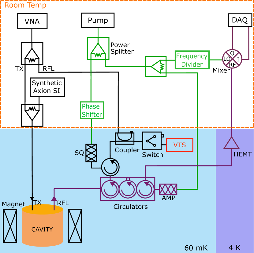
Figure 1: Simplified version of the HAYSTAC receiver described in [24]. In black are inputs to the system which can be sent to either the cavity’s transmission (TX) or reflection (RFL) port. These are used for characterizing the system with a VNA and for injecting synthetic axion signals into the system. The green lines indicate the path of the pump tone used by both the JPAs and the IQ-mixer. Finally, shown in purple is the readout path which extracts and amplifies signals from the cavity for readout.

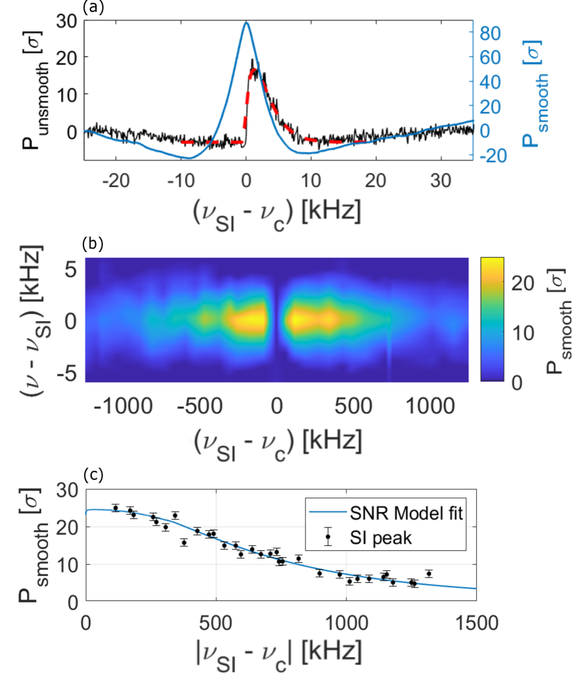
Figure 2: (a) Combined and normalized power spectrum for a synthetic axion signal injected at 4.459220 GHz during Phase IId, both with (blue solid line) and without (black solid line) ALS smoothing, compared to the expected ALS (red dashed line). (b) As expected, the observed power in the individual power spectrum is larger for tuning steps where the detuning of the signal from the cavity mode is smaller. (c) The peak power of the injected signal observed at each of these tuning steps (black dots) follows the scaling predicted by the SNR model (blue solid line). The powers at detunings $<$$45\text{\,}\mathrm{kHz}$ are removed as this is outside of the analysis band.

During standard data-taking, a fully automated script first tunes the cavity’s resonance by rotating the tuning rod, producing a frequency step size of $\sim$$80\text{\,}\mathrm{k}\mathrm{H}\mathrm{z}$, and then sets the pump frequency of the JPAs to twice the cavity frequency measured by the VNA. To ensure optimal sensitivity, the phase shift between the two JPAs along with the JPA bias currents and pump powers are tuned to optimize the squeezing. At each tuning step, the digitizer records data in $10\text{\,}\mathrm{m}\mathrm{s}$ segments at a sampling rate $\geq$ $5\text{\,}\mathrm{M}\mathrm{H}\mathrm{z}$ and computes the average power spectral density (PSD) over time $\tau$. During Phase IIc/d an integration time of 20 minutes was used, lower than the 60 minutes used in Phase IIa/b to allow for a larger range of frequencies to be covered.

	Op. [days]	$\Delta\nu$ [MHz]	$|g_{\gamma}/g_{\text{KSVZ}}|$	Cand.	RFI	Def.	SI
a	106	73	2.05	32	-	5	-
b	53	64	1.96	37	-	1	-
c	72	184	3.04	98	7	8	3
d	111	229	3.06	120	5	16	3

Table 1: Summary of HAYSTAC’s Phase II operations showing total operational days, frequency coverage, and the average $|g_{\gamma}|$ which would produce a 5.1$\sigma$ signal for the initial scans. Also shown are the total number of rescan candidates along with the individual contributions from the non-statistical fluctuations (RF interference, deficits, and synthetic axion SI) described in the text.

Calibration of the noise performance follows a similar routine to that described in [21, 24, 27], with the system noise expressed using single-quadrature spectral densities. The calibration starts with a standard Y-factor measurement with the JPAs detuned from the cavity to extract the added noise of the amplification chain, $N_{a}$, referred to the input of the AMP. This is achieved by comparing the output noise for two different input loads. One thermalized to the mixing chamber at $60\pm$$1\text{\,}\mathrm{m}\mathrm{K}$, and the other thermalized to a variable temperature stage (VTS) held at $290\pm$$10\text{\,}\mathrm{m}\mathrm{K}$. This measurement is repeated approximately once per nine tuning steps during normal operations to capture potential variations with frequency and time. Over the range covered in Phase IIc/d, $N_{a}$ was observed to vary between $0.01<N_{a}<0.18$ quanta with an average value of $N_{a}=0.08\pm 0.07$ quanta over the analysis band, with this and subsequent error bars representing systematic error. This agrees, within the uncertainty, to the specifications of the HEMT noise which is expected to be the dominant contribution. The above measurement of $N_{a}$ requires knowing the transmission efficiency between the input load and the AMP. Following a similar routine to [26], this is measured in two steps by varying which JPA is used as the main amplifier to decouple the efficiency between the input load and the SQ ($\lambda$) from the efficiency between the SQ and AMP ($\eta$). To account for possible frequency-dependent variations, this measurement is repeated over the full range of frequencies covered in Phase IIc/d, in steps of $3\text{\,}\mathrm{MHz}$, outside of normal operations. Over this range, $\lambda$ is found to be generally frequency-independent, with an average value of $\lambda=0.67\pm 0.05$, while $\eta$ was found to vary by 12$\%$ with an average value of $\eta=0.65\pm 0.03$.

Similar to Phase IIa/b, the observed noise contribution of the cavity, $S_{c}$, is larger than would be expected for a cavity thermalized to the mixing chamber. This is quantified by periodically comparing the PSD with and without the cavity present. During Phase IIc/d, $S_{c}$ exhibited repeatable variations with the TM₀₁₀ frequency, with $S_{c}$ ranging between $0.43<\mbox{$S_{c}$}<1.20$ quanta and having an average of $S_{c}$ $=0.71\pm 0.15$ quanta over the full range of Phase IIc/d. While the cause of this excess noise is still being investigated, it has previously been attributed to poor thermalization of the tuning rod but could also be the result of noise coupling through one of the cavity ports.

The final step in characterizing the performance is a measurement of the noise reduction from squeezing. Following [26, 21, 24], this is quantified by comparing the PSD taken with and without the SQ. Measurements taken over the frequency range of Phase IIc/d, with the JPAs tuned away from the cavity resonance, show off-resonant squeezing ranging between $3.5<S<4.0$ dB, in agreement with the expected performance given the measured values of $\eta$ and $N_{a}$. However, the observed squeezing during normal operations, with the JPAs tuned to match the cavity frequency, was lower than expected from the off-resonant measurements. It is suspected that the additional noise, with a similar shape to the cavity Lorentzian, is caused by mechanical vibrations of the cavity tuning rod or the antenna. These vibrations cause the TM₀₁₀ mode to oscillate at a rate below $\sim$$200\text{\,}\mathrm{Hz}$, resulting in dephasing of the squeezed state between the two JPAs relative to the optimal $90\text{\,}\mathrm{\SIUnitSymbolDegree}$ phase difference. Because this noise varies with both time and frequency, a measurement with and without SQ is taken before each power spectrum to extract the squeezing as a function of detuning. To understand the impact on the sensitivity, this can be translated into a scan rate enhancement ($E$) relative to operation without squeezing [26]. In the absence of additional noise from vibrations, an enhancement between $1.8<\mbox{$E$}<2.0$ would be expected given the off-resonant performance. However, taking into account the observed noise in Phase IIc/d, the average enhancement achieved was $\mbox{$E$}=1.7$ with the enhancement varying between $1.3<\mbox{$E$}<2.0$ over the full operating range.

Analysis and Results – Data recorded by the digitizer is analyzed largely following the procedure described in [24, brubaker2017analysis], which starts with a set of data quality cuts to remove spectra that exhibit poor or anomalous behavior such as unstable gains, non-optimal squeezing, or degraded cavity performance. In total, these cuts remove $\sim$3$\%$ of recorded spectra. The remaining spectra are then processed with a Savitzky-Golay (SG) filter to remove structures wider than expected from the ALS. In the absence of a signal, the processed spectra are approximately Gaussian distributed with $\mu=0$ and $\sigma=1/\sqrt{\Delta_{b}\tau}$, where $\Delta_{b}$ = $100\text{\,}\mathrm{H}\mathrm{z}$ is the frequency resolution of the FFT. The spectra are then scaled by the maximum likelihood weights given by the signal-to-noise (SNR), aligned by their RF frequency, and summed to produce a single grandspectrum showing the observed power excess at each probed frequency. This spectrum is then smoothed via cross-correlation with the expected ALS and normalized such that it is approximately $\mathcal{N}(0,1)$ distributed.

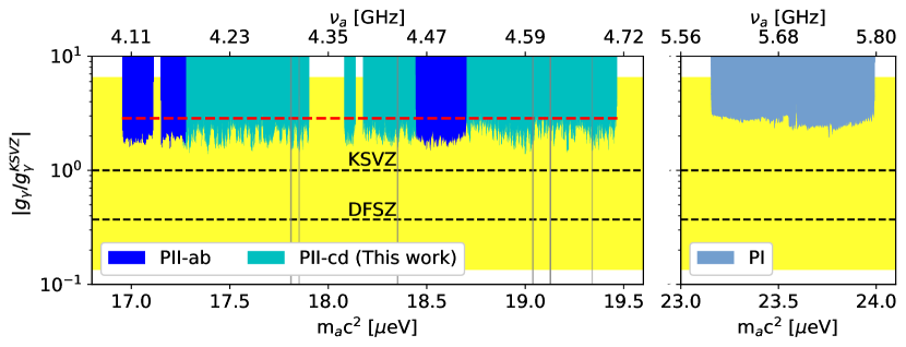
Figure 3: Exclusion on the axion-photon coupling for this work (Phase IIc/d) shown alongside previous results from Phase IIa/b [21, 24] and Phase I [29, 28], with the dashed red line denoting the joint $90\text{\,}\mathrm{\char 37\relax}$ aggregate exclusion level of 2.86$\times$$|g_{\gamma}^{\text{KSVZ}}|$ for all of Phase II. Marked in gray are regions removed from the exclusion due to RFI contamination described in the text. The QCD axion model band is shown in yellow [Diluzio2020modelband], with the benchmark KSVZ and DFSZ models [14, 15, 16, 17] shown as black dashed lines.

$\nu$ [GHz]	Persist	0-Field	Amb. Veto
4.676364	✓	X	X
4.625081	X	X	X
4.625005	X	✓	X
4.624968	X	✓	X
4.624940	X	✓	X
4.603546	X	X	X
4.603480	X	X	X
4.437575	✓	X	X
4.437503	✓	X	X
4.316643	X	✓	X
4.306543	X	✓	X
4.306533	X	X	X

Table 2: Summary table of the 12 RFI detected in Phase IIc/d showing the three pass (✓)/fail (X) checks required to be considered an axion. This includes persistence upon further observation (Persist), failure to persist when the magnetic field is absent (0-Field), and lack of clear correlation to an ambient RF signal (Amb. Veto). Each candidate failed at least one check and was eliminated as an axion signal.

Using the grandspectrum produced from an initial scan, potential candidates are identified as excesses $\geq 3.468\sigma$, corresponding to a $10\%$ two-scan false negative rate for a 5.1$\sigma$ target significance in the Frequentist framework used in [29, 28, brubaker2017analysis]. Any candidate found above this threshold was further interrogated in rescans to test for persistence, as expected for an axion signal. This procedure identified 98 candidates for Phase IIc and 120 for Phase IId. While most of these candidates are likely the result of random fluctuations in the noise, three distinct populations of non-Gaussian noise were identified as summarized in Table 1.

The first group were the six synthetic axion SIs described in the previous section. Each SI candidate was identified above the threshold at the injected frequency and exhibited both the correct frequency distribution and expected scaling with cavity detuning, which match the SNR model detailed in [24] as shown in Fig. 2 for one of the injections. Once identified and validated, data in the $10\text{\,}\mathrm{k}\mathrm{H}\mathrm{z}$ ($\sim$2$\delta\nu_{a}$) window around each candidate was cut and later filled in during rescans. Next was a group of candidates, also seen in Phase IIa/b, presenting as large ($\sim$$40\text{\,}\mathrm{k}\mathrm{H}\mathrm{z}$) power “deficits” exceeding the $5.1\sigma$ target significance but in the negative direction. While their source is unknown, no such candidate has been found to repeat upon rescan. Data cuts of $200\text{\,}\mathrm{k}\mathrm{H}\mathrm{z}$ were conservatively applied to remove data around each candidate and the gaps were later filled in upon rescan. The final group are a set of large but narrow ($\sim$$1\text{\,}\mathrm{k}\mathrm{H}\mathrm{z}$) excesses which are clearly visible above the target significance in both the grandspectrum and the individual spectra from multiple tuning steps, with their clear signature prompting suspicion of RF interference (RFI) from environmental sources. Upon probing each candidate a total of three times with field on at $8\text{\,}\mathrm{T}$, only three candidates persisted in all scans as summarized in Table 2. Each candidate was also scanned at zero-field, with the three persistent candidates all still visible in the spectrum. The five candidates which did not persist at zero-field also failed to persist during the three rescans taken at $8\text{\,}\mathrm{T}$, likely indicating a change in the source or in the coupling to the detector rather than an axion signal. The final step in confirming these excesses as RFI was to check against an ambient RF detector consisting of a simple antenna. All 12 candidates had a clear correlation to an ambient signal within $\delta_{\nu_{a}}$$\sim$ $5\text{\,}\mathrm{k}\mathrm{H}\mathrm{z}$, ruling out axions and other sources such as Dark Photons [darkphoton_bandbook, darkphoton_sumita]. The exact origin of these signals is unknown, but our detection band is between 4–5 GHz, a popular band for communication [wifi]. To remove them from the spectrum, data in the $10\text{\,}\mathrm{k}\mathrm{H}\mathrm{z}$ window around each RFI were cut, amounting to a $\sim$0.02$\%$ loss in total frequency coverage in Phase II.

After completing rescans, all candidates either failed to persist or were ruled out through the cross-checks described above. Given the absence of an axion signal, an exclusion limit on $|g_{\gamma}|$ is set using the Bayesian framework outlined in [palken2020improved] giving both a $10\text{\,}\mathrm{\char 37\relax}$ prior update contour for each scanned frequency along with an aggregate exclusion at the $90\text{\,}\mathrm{\char 37\relax}$ level over the entire range. Aggregated separately, couplings $|g_{\gamma}|\geq$ 2.96$\times$$|g_{\gamma}^{\text{KSVZ}}|$ are excluded between 18.71–19.46 $\mu$eV in Phase IIc and couplings $|g_{\gamma}|\geq$ 2.75$\times$$|g_{\gamma}^{\text{KSVZ}}|$ are excluded between 17.28–18.44 $\mu$eV in Phase IId (excluding the mode crossings at 17.89–18.08 $\mu$eV and 18.13–18.18 $\mu$eV and the 12 RFI sources). In addition, the individual sub-phases can be combined to find a joint aggregate exclusion level of 2.86$\times$$|g_{\gamma}^{\text{KSVZ}}|$ over the entire range covered in Phase II. These results, along with previous HAYSTAC results, are plotted in Fig. 3.

Conclusion and Outlook – The results presented in this Letter show the combined search of HAYSTAC’s Phase II operation, which covers $550\text{\,}\mathrm{MHz}$ of parameter space in the extended QCD model band including $413\text{\,}\mathrm{MHz}$ of newly explored parameter space. This result showcases the SSR’s capability to operate effectively across a wide range of parameter space. Future operations will focus on expanding HAYSTAC to higher frequencies with a new set of JPAs, a new cavity design [Simanovskaia:2020hox], techniques to mitigate squeezing degradation related to vibration, and a new readout involving state swapping and two-mode squeezing to further speed up the scan rate [Wurtz_2021, Jiang_2023].

HAYSTAC is supported by the National Science Foundation under grants PHY-1701396, PHY-1607223, PHY-1734006, PHY-2011357, PHY-2309631, PHY-2209556, the Heising-Simons Foundation under grants 2014-0904 and 2016-044, and the Sloan Foundation under grant FG-2022-19263 141275. We thank Kyle Thatcher and Calvin Schwadron for their work on the design and fabrication of the SSR mechanical components, Felix Vietmeyer for his work on the room temperature electronics, and Steven Burrows for his graphical design work. We thank Vincent Bernardo and the J. W. Gibbs Professional Shop as well as Craig Miller and Dave Johnson for their assistance with fabricating the system’s mechanical components. We also wish to thank the Cory Hall Machine shop at UC Berkeley and the efforts of Sergio Velazquez for fabricating several of the prototype components tested here. We thank Dr. Matthias Buehler of low-T Solutions for cryogenics advice. Finally, we thank the Wright laboratory for housing the experiment and providing computing and facilities support.

References

- Peccei and Quinn [1977a] R. D. Peccei and H. R. Quinn, conservation in the presence of pseudoparticles, Phys. Rev. Lett. 38, 1440 (1977a).
- Peccei and Quinn [1977b] R. D. Peccei and H. R. Quinn, Constraints imposed by conservation in the presence of pseudoparticles, Phys. Rev. D 16, 1791 (1977b).
- Weinberg [1978] S. Weinberg, A New Light Boson?, Phys. Rev. Lett. 40, 223 (1978).
- Abbott and Sikivie [1983] L. F. Abbott and P. Sikivie, A Cosmological Bound on the Invisible Axion, Phys. Lett. B 120, 133 (1983).
- Preskill et al. [1983] J. Preskill, M. B. Wise, and F. Wilczek, Cosmology of the Invisible Axion, Phys. Lett. B 120, 127 (1983).
- Dine and Fischler [1983] M. Dine and W. Fischler, The Not So Harmless Axion, Phys. Lett. B 120, 137 (1983).
- Gorghetto and Villadoro [2019] M. Gorghetto and G. Villadoro, Topological Susceptibility and QCD Axion Mass: QED and NNLO corrections, JHEP 03, 033, arXiv:1812.01008 [hep-ph] .
- Klaer and Moore [2017] V. B. . Klaer and G. D. Moore, The dark-matter axion mass, JCAP 11, 049, arXiv:1708.07521 [hep-ph] .
- Buschmann et al. [2020] M. Buschmann, J. W. Foster, and B. R. Safdi, Early-Universe Simulations of the Cosmological Axion, Phys. Rev. Lett. 124, 161103 (2020), arXiv:1906.00967 [astro-ph.CO] .
- Saikawa et al. [2024] K. Saikawa, J. Redondo, A. Vaquero, and M. Kaltschmidt, Spectrum of global string networks and the axion dark matter mass (2024), arXiv:2401.17253 [hep-ph] .
- O’Hare et al. [2022] C. A. J. O’Hare, G. Pierobon, J. Redondo, and Y. Y. Y. Wong, Simulations of axionlike particles in the postinflationary scenario, Phys. Rev. D 105, 055025 (2022), arXiv:2112.05117 [hep-ph] .
- Buschmann et al. [2022] M. Buschmann, J. W. Foster, A. Hook, A. Peterson, D. E. Willcox, W. Zhang, and B. R. Safdi, Dark matter from axion strings with adaptive mesh refinement, Nature Commun. 13, 1049 (2022), arXiv:2108.05368 [hep-ph] .
- Rybka [2024] G. Rybka, Axion dark matter searches above 1 eV, Nucl. Phys. B 1003, 116481 (2024).
- Kim [1979] J. E. Kim, Weak Interaction Singlet and Strong CP Invariance, Phys. Rev. Lett. 43, 103 (1979).
- Shifman et al. [1980] M. A. Shifman, A. I. Vainshtein, and V. I. Zakharov, Can Confinement Ensure Natural CP Invariance of Strong Interactions?, Nucl. Phys. B 166, 493 (1980).
- Dine et al. [1981] M. Dine, W. Fischler, and M. Srednicki, A Simple Solution to the Strong CP Problem with a Harmless Axion, Phys. Lett. B 104, 199 (1981).
- Zhitnitsky [1980] A. R. Zhitnitsky, On Possible Suppression of the Axion Hadron Interactions. (In Russian), Sov. J. Nucl. Phys. 31, 260 (1980).
- Patrignani et al. [2016] C. Patrignani et al. (Particle Data Group), Review of Particle Physics, Chin. Phys. C 40, 100001 (2016).
- Haus and Mullen [1962] H. A. Haus and J. A. Mullen, Quantum noise in linear amplifiers, Phys. Rev. 128, 2407 (1962).
- Caves [1982] C. M. Caves, Quantum limits on noise in linear amplifiers, Phys. Rev. D 26, 1817 (1982).
- Backes et al. [2021] K. M. Backes et al. (HAYSTAC), A quantum-enhanced search for dark matter axions, Nature 590, 238 (2021), arXiv:2008.01853 [quant-ph] .
- Backes [2021] K. M. Backes, A Quantum-Enhanced Search for Dark Matter Axions, Ph.D. thesis, Yale University (2021).
- Palken [2020] D. A. Palken, Enhancing the scan rate for axion dark matter: Quantum noise evasion and maximally informative analysis, Ph.D. thesis, University of Colorado Boulder (2020).
- Jewell et al. [2023] M. J. Jewell et al. (HAYSTAC), New results from HAYSTAC’s phase II operation with a squeezed state receiver, Phys. Rev. D 107, 072007 (2023), arXiv:2301.09721 [hep-ex] .
- Yamamoto et al. [2008] T. Yamamoto et al., Flux-driven Josephson parametric amplifier, Appl. Phys. Lett. 93, 042510 (2008).
- Malnou et al. [2019] M. Malnou, D. A. Palken, B. M. Brubaker, L. R. Vale, G. C. Hilton, and K. W. Lehnert, Squeezed vacuum used to accelerate the search for a weak classical signal, Phys. Rev. X 9, 021023 (2019), [Erratum: Phys.Rev.X 10, 039902 (2020)], arXiv:1809.06470 [quant-ph] .
- Malnou et al. [2018] M. Malnou, D. A. Palken, L. R. Vale, G. C. Hilton, and K. W. Lehnert, Optimal Operation of a Josephson Parametric Amplifier for Vacuum Squeezing, Phys. Rev. Appl. 9, 044023 (2018), arXiv:1711.02786 [quant-ph] .
- Brubaker et al. [2017a] B. M. Brubaker et al., First results from a microwave cavity axion search at 24 eV, Phys. Rev. Lett. 118, 061302 (2017a), arXiv:1610.02580 [astro-ph.CO] .
- Zhong et al. [2018] L. Zhong et al. (HAYSTAC), Results from phase 1 of the HAYSTAC microwave cavity axion experiment, Phys. Rev. D 97, 092001 (2018), arXiv:1803.03690 [hep-ex] .