Revisiting Local PageRank Estimation on Undirected Graphs: Simple and Optimal
Abstract.
We propose a simple and optimal algorithm, BackMC, for local PageRank estimation in undirected graphs: given an arbitrary target node in an undirected graph comprising nodes and edges, BackMC accurately estimates the PageRank score of node while assuring a small relative error and a high success probability. The worst-case computational complexity of BackMC is upper bounded by , where denotes the minimum degree of , and denotes the degree of , respectively. Compared to the previously best upper bound of (VLDB ’23), which is derived from a significantly more complex algorithm and analysis, our BackMC improves the computational complexity for this problem by a factor of with a much simpler algorithm. Furthermore, we establish a matching lower bound of for any algorithm that attempts to solve the problem of local PageRank estimation, demonstrating the theoretical optimality of our BackMC. We conduct extensive experiments on various large-scale real-world and synthetic graphs, where BackMC consistently shows superior performance.
1. Introduction
PageRank is a celebrated metric for assessing node centrality in graphs, originally introduced by Google for ranking web pages based on their prominence within the web network (page1999pagerank, ; brin1998anatomy, ). Over the past two decades, PageRank has evolved into one of the most popular graph centrality metrics, with widespread applications across diverse fields. These include social network analysis (gupta2013wtf, ), spam detection (gyongyi2004combating_pagerank_spam, ), recommender systems (gori2007itemrank, ), graph representation learning (chen2020GBP, ; klicpera2019APPNP, ), chemical informatics (mooney2012molecularnetworks, ), and bioinformatics (morrison2005generank, ), and more (gleich2015beyondtheweb, ). The computation of PageRank has become a fundamental aspect of modern network analysis.
In recent years, the exponential growth in network sizes has sparked significant interest in the field of local PageRank estimation (chen2004local, ; bar2008reversePageRank, ; setpush2023VLDB, ; bressan2018sublinear, ; bressan2023sublinear, ; lofgren2014FastPPR, ; lofgren2016BiPPR, ; lofgren2015bidirectional_undirected, ; wang2020RBS, ; lofgren2013personalized, ; andersen2007contribution, ). This problem focuses on the approximation of a given target node’s PageRank score, with the goal of exploring only a small portion of the graph. Various practical applications illustrate the utility of local PageRank estimation. For example, in recommender systems, there is a growing need to quickly approximate the PageRank scores of individual users during online operations, as opposed to performing time-consuming global computations of determining all nodes’ PageRank scores within a graph (chen2004local, ). Similarly, in web search scenarios, website owners who are interested in enhancing their search engine rankings may only seek the PageRank score of their specific websites, not those of the entire web (bar2008reversePageRank, ). Additionally, in social networks, users often desire to gauge their PageRank-based popularity by efficiently probing the friendship graph, rather than having to traverse the entire networkr (setpush2023VLDB, ; bar2008reversePageRank, ). Therefore, it is imperative to have highly efficient algorithms for local PageRank estimation.
This paper focuses on local PageRank estimation in undirected graphs 111It’s important to note, as formally established in (grolmusz2015note, ), that the PageRank scores in undirected graphs are not simply proportional to node degrees, despite common misconceptions to the contrary often cited in the literature. . We aim to address the problem of computing, with probability , a multiplicative -approximation of the PageRank score for a given target node in an undirected graph comprising nodes and edges. Both and are constants set within the range (e.g., ). This problem is of great importance from both theoretical and practical aspects.
Theoretical Motivations. Existing studies on local PageRank estimation can be broadly divided into two categories. The first category focuses on the approximation of a single node’s PageRank score on general directed graphs (bressan2018sublinear, ; bressan2023sublinear, ; wang2020RBS, ; lofgren2014FastPPR, ; lofgren2016BiPPR, ), while the second specifically targets undirected graphs (setpush2023VLDB, ; lofgren2015bidirectional_undirected, ). For directed graphs, the best-known lower bound of for the worst-case computational complexity was established by Bressan, Peserico, and Pretto (bressan2018sublinear, ; bressan2023sublinear, ), where denotes the maximum outdegree of . This lower bound indicates the improbability of achieving a complexity bound of even on very sparse directed graphs. Surprisingly, on undirected graphs, a recent work (setpush2023VLDB, ) shows that the computational complexity of local PageRank approximation can be improved to by leveraging the symmetry of PageRank vectors in undirected graphs 222 For readability, we hide multiplicative factors depending on the parameters and in the notation, following (bressan2018sublinear, ; bressan2023sublinear, ; setpush2023VLDB, ; wang2020RBS, ). These factors in our upper bound can be found in Section 4. . Here, denotes the degree of the target node in the undirected graph . We note that this upper bound is even asymptotically better than the lower bound established for directed graphs. This encouraging result underscores the theoretical significance and necessity of exploring the complexity bounds of local PageRank estimation on undirected graphs. However, the question of whether this upper bound can be further improved remains open due to the lack of lower bounds for undirected graphs (setpush2023VLDB, ). To the best of our knowledge, only a trivial lower bound of has been established over the years. This gap in understanding motivates our exploration in this area.
Applications Significance. Local estimation of PageRank scores on undirected graphs is a versatile tool with a range of applications. A typical example is its use in Graph Neural Networks (GNNs). The majority of GNN models are primarily designed for undirected graphs, aiming to derive low-dimensional latent representations of all training nodes from structural and feature information. A message-passing mechanism is typically employed in existing GNN models for feature propagation. In particular, a line of research (chen2020GBP, ; klicpera2019APPNP, ; Bojchevski2020PPRGo, ; wang2021AGP, ) utilizes PageRank queries for efficient feature propagation, where the initial feature vector serves as the preference vector for PageRank computations (as detailed in Section 2). In these models, feature propagation is essentially akin to computing PageRank scores for a selected group of nodes in semi-supervised learning tasks, like community classification on a billion-scale graph Friendster (chen2020GBP, ), where feature vector entries are binary and the number of training nodes is small. Thus, an efficient local PageRank algorithm can greatly enhance the scalability of GNN models in these contexts. Moreover, the simulation of random walks in undirected graphs is a prevalent approach widely adopted in various graph learning tasks (chen2020GBP, ; Zeng2020graphsaint, ; wang2021AGP, ; perozzi2014deepwalk, ). While prior studies have demonstrated the empirical efficacy of this method, they fall short of providing a theoretical foundation for the optimality of generating random walks in undirected settings. This paper establishes that merely generating random walks from a specified target node achieves the optimal complexity for local PageRank computation. Our findings aim to lay a theoretical foundation for the efficacy of random walk simulations in undirected graphs, thereby informing the design of graph learning methods tailored to such graphs.
1.1. Our Contributions
In this paper, we address the problem of locally estimating the PageRank score of a target node in an undirected graph . We achieve the following contributions:
-
•
We introduce BackMC, an algorithm that achieves the worst-case computational complexity of , where represents the minimum degree of the graph , denotes the degree of the target node , and is the total number of edges in . This computational complexity notably improves upon the previous best upper bound of , as documented for the SetPush algorithm (setpush2023VLDB, ), by a factor of . Remarkably, although the complexity result of SetPush is derived from a significantly complex analysis, the algorithm structure and theoretical analysis of our BackMC exhibit a surprising simplicity.
-
•
We improve the lower bound for this problem from a trivial bound of to . The matching upper and lower bounds demonstrate that our BackMC has been optimal.
-
•
Beyond its theoretical optimality, BackMC distinguishes itself with a clean algorithm structure and straightforward implementation, and thus achieves exceptional empirical performance. We conduct extensive experiments on large-scale real-world and synthetic graphs, and BackMC consistently outperforms all baseline algorithms. Notably, it surpasses SetPush in both efficiency and accuracy by up to three orders of magnitude.
2. Preliminaries
We denote the underlying undirected graph as , with and representing the adjacency and degree matrices of , respectively. The graph consists of nodes and edges. For any undirected edge in , nodes and are termed as neighbors. For a node in , the set of its neighbors is denoted as , and its degree is represented by . We further define and as the maximum and minimum degrees of , respectively. We list frequently used notations in Table 1 for quick reference.
| Notation | Description |
| undirected graph with node set and edge set | |
| adjacency and degree matrices of | |
| numbers of nodes and edges in | |
| set of neighbors of | |
| degree of node | |
| maximum degree of | |
| minimum degree of | |
| PageRank vector | |
| real and estimated PageRank scores of node | |
| Personalized PageRank score of node w.r.t node | |
| teleport probability in defining PageRank | |
| relative error parameter | |
| failure probability parameter |
2.1. PageRank
The PageRank vector of graph is defined as the stationary distribution of the PageRank Markov chain (page1999pagerank, ; brin1998anatomy, ), satisfying:
| (1) |
where is the teleport probability, and is an all-one column vector of length . The vector is termed as the preference or personalized vector in PageRank.
For any node in , the PageRank score of , denoted by , corresponds to the entry in associated with node . It is well known that equals the probability that an -discounted random walk, starting from a random source node uniformly chosen in , terminates at node (page1999pagerank, ; brin1998anatomy, ). Here, an -discounted random walk is a type of random walk where the length of the walk is a random variable that takes on value with probability for each . In other words, at each step of the -discounted random walk, there is a probability of that the walk will terminate, and a probability of that the walk will continue to the next step.
Equation (1) implies that the following recursive equality holds for any node .
| (2) |
Moreover, Wang and Wei (setpush2023VLDB, ) demonstrate that for any node ,
| (3) |
We present the proof below for the sake of completeness.
Proof of Equation (3).
By Equation (2), we have for any node . Applying into Equation (2) further yields that
| (4) |
In particular, by the Cauchy-Schwarz inequality, we have
It is important to note that , therefore giving that . By Plugging into Inequality (4), we have
By the AM-GM inequality, we further have
Combining these results gives the claimed inequality. ∎
2.2. Personalized PageRank
Personalized PageRank (PPR) serves as an ego-centric counterpart to PageRank, quantifying the probability that an -discounted random walk, starting from a source node , terminates at a target node . This is expressed as the PPR score of with respect to , symbolized by . It follows naturally that the PageRank score of is the average of across all nodes in the graph, formalized as
| (5) |
Specifically, on undirected graphs, PPR scores exhibit symmetry for any pair of nodes :
| (6) |
The proof of Equation (6) is detailed in (lofgren2015bidirectional_undirected, ).
2.3. Computational Model
In this paper, we adopt the standard RAM model for computational complexity. To establish lower bounds, we consider query complexity under the standard arc-centric graph access model (goldreich1998property, ; goldreich2002property, ), where local algorithms can access the underlying graph only through a graph oracle via several local queries and a global operation. This setting aligns well with practical situations with massive-scale network structures. Specifically, for undirected graphs, the graph oracle supports three elementary query operations, each taking unit time: , which returns ; , which returns the -th node in ; , which returns a random node uniformly chosen from . Algorithm 2 is an example on how to leverage these query operations to sample random walks in the graph. The query complexity of a graph algorithm is defined as the number of elementary query operations invoked on the graph oracle. It is worth noting that the query complexity of an algorithm serves as a lower bound for its computational complexity.
3. Related Work
The problem of estimating PageRank scores locally was introduced in (chen2004local, ), and, in its various forms, has received considerable attention over the past decade (chen2004local, ; bar2008reversePageRank, ; setpush2023VLDB, ; bressan2018sublinear, ; bressan2023sublinear, ; lofgren2014FastPPR, ; lofgren2016BiPPR, ; lofgren2015bidirectional_undirected, ; wang2020RBS, ; lofgren2013personalized, ; andersen2007contribution, ; fogaras2005MC, ). These methods can be broadly categorized into three groups based on their underlying techniques. A summary of their complexity bounds is provided in Table 2. In this section, we will briefly review these methods. Section 4 will delve into the limitations of existing methods and offer a detailed comparison with our BackMC algorithm.
| Method | Complexity Bound | Notes |
| PowerIteration (page1999pagerank, ) | ||
| BackwardPush (lofgren2013personalized, ) | ||
| MC (fogaras2005MC, ) | ||
| RBS (wang2020RBS, ) | ||
| Undir-BiPPR (lofgren2015bidirectional_undirected, ) | ||
| BPPPush (bressan2018sublinear, ) | ||
| (bressan2023sublinear, ) | ||
| SetPush (setpush2023VLDB, ) | ||
| BackMC (Ours) | ||
| Lower Bound (Ours) |
The first category (fogaras2005MC, ; avrachenkov2007monte, ; borgs2012sublinear, ; borgs2014multiscale, ) is inspired by the probabilistic interpretation of PageRank scores. The seminal work by Fogaras et al. (fogaras2005MC, ) introduced a Monte Carlo (MC) method that initiates a series of -discounted random walks across the graph , where each random walk is generated from a uniformly random source node in . The MC method calculates the proportion of walks that terminate at the given target node , utilizing this ratio to approximate . To achieve a multiplicative -approximation of with probability , the expected computational complexity of the MC method is upper bounded by . This result is applicable to both directed and undirected graphs.
Another line of research (andersen2007contribution, ; lofgren2013personalized, ; wang2020RBS, ; setpush2023VLDB, ) focuses on the estimation of for all , using Equation (5) to derive an estimate for . These algorithms start with one unit of probability mass at node and perform a sequence of push operations to distribute the probability mass across the graph . The push operation, applied to node , redistributes the probability mass from node to its neighbors, following the recurrence equation in Equation (2). The seminal paper (andersen2007contribution, ) in this category introduces the ApproxContributions algorithm, which achieves a worst-case computational complexity of for determinsitically computing a multiplicative -approximation of . It is worth noting that this result is only applicable to undirected graphs. On directed graphs, the running time of ApproxContributions can only be bounded by in expectation over a uniform random choice of . Subsequent studies, such as the BackwardPush algorithm by Lofgren and Goel (lofgren2013personalized, ), improved the framework of ApproxContributions to achieve a worst-case computational complexity of on undirected graphs and an average running time of over all on directed graphs. A recent advancement, RBS (wang2020RBS, ), further improves the worst-case computational complexity of this problem to . This result applies to both directed and undirected graphs. The key idea of RBS is to pre-sort the neighbors of each node in ascending order of their degrees and, in each push operation, propagate probability mass only to neighbors with small degrees. The SetPush algorithm (setpush2023VLDB, ) achieves the best-known worst-case complexity of for estimating on undirected graphs. The algorithm critically depends on the symmetry of PPR scores in undirected graphs. It employs a complex push strategy to estimate for all , and then derives the approximation of using the equation , as inferred from Equation (5) and (6).
Additionally, a set of papers presents novel results by combining the Monte Carlo method and push operations. This idea was introduced in the FastPPR algorithm (lofgren2014FastPPR, ), and further refined in the BiPPR algorithm (lofgren2016BiPPR, ), both designed for directed graphs. An alternative version of BiPPR, referred to as Undir-BiPPR, has been tailored for undirected graphs. Undir-BiPPR achieves a worst-case computational complexity of for estimating . In the recent work by Bressan, Peserico, and Pretto (bressan2018sublinear, ), a worst-case computational complexity of was achieved for general directed graphs. Subsequently, this bound was further improved to in (bressan2023sublinear, ), establishing itself as the best-known worst-case complexity bound for local PageRank approximation in directed graphs.
As for lower bounds, Bar-Yossef and Mashiach (bar2008reversePageRank, ) have proven that, in directed graphs, the lack of operation imposes a lower bound of on the query complexity for locally approximating . Moreover, Bressan, Peserico, and Pretto (bressan2018sublinear, ) have shown that a lower bound of elementary query operations is necessary in the worst case to estimate within a multiplicative factor with probability in directed graphs. However, the lower bounds pertaining to the estimation of on undirected graphs remain unclear.
4. Algorithm
This section presents our BackMC algorithm. We demonstrate that BackMC can achieve the following upper bound simply by generating a series of -discounted random walks from node .
Theorem 1.
Given an undirected graph and a target node , the expected computational complexity of BackMC for computing a multiplicative -approximation of with probability at least is .
Algorithm 1 provides the pseudocode for BackMC. At the heart of Algorithm 1 is the function, responsible for simulating an -discounted random walk from node in . We define the indicator variable , which equals if . We also compute a temporary estimator . We invoke for times to obtain independent realizations of , and take their average as the final estimate for .
4.1. Analysis
This section presents the proof of Theorem 1. It is straightforward that is a Bernoulli random variable that takes on value with probability . Therefore, is an unbiased estimator for since , as inferred from Equation (5) and (6). It is important to note that BackMC computes by averaging independent realizations of . Thus, also emerges as an unbiased estimator for .
We now proceed to bound the variance of the estimator generated by BackMC. It is well-known that the variance of the Bernoulli random variable is given by . It is worth noting that for all , the random variables are negatively correlated since an -discounted random walk can only terminate at a single node. Consequently, we have
By utilizing Equation (6), we can further derive that
where we employ Equation (5) to assert that . Recall that BackMC computes as the average of independent realizations of . As a result, we can bound the variance of the estimator in BackMC as .
Therefore, with , Chebyshev’s inequality guarantees that
Given that (from Inequality (3)), we can ensure that by setting .
To further reduce the failure probability to , we use the Median trick. The core idea is to independently run BackMC multiple times and take the median of the resulting as the final estimate for . Specifically, we use to denote the number of BackMC runs. For each integer , we define the indicator variable , which equals if the -th run fails to achieve . Based on the earlier proof, we have when . Furthermore, we define as the count of times BackMC fails to produce a satisfactory approximation of . The probability that the median of these estimates is not a multiplicative -approximation of can thus be quantified as . Given that , by Hoeffding’s inequality, yields:
As a consequence, the total number of -discounted random walks generated in turns out to be
We observe that the expected length of each -discounted random walk is . Consequently, the expected running time of the entire process can be upper bounded by
This completes the proof of Theorem 1.
Remark. We note that the setting of requires explicit knowledge of and . As demonstrated in (bressan2018sublinear, ; bressan2023sublinear, ; dagum2000optimal, ), this requirement can be easily waived. To achieve this, we run BackMC with an initial value for (e.g., ). If we find that during the process, standard concentration bounds allow us to safely terminate BackMC and return as a multiplicative -approximation of . In case this condition is not met, we double the value of and repeat the process. This modification does not affect the validity of Theorem 1.
4.2. Comparison with Previous Methods
This subsection presents a thorough comparison between BackMC and previous methods.
First, considering SetPush, it achieves the best-known worst-case complexity of for this problem, with a hidden multiplicative factor of . In contrast, BackMC has a worst-case computational complexity of , with a more favorable multiplicative dependency on of . This complexity surpasses that of SetPush by a factor of . Additionally, the improvement in the factor can be significant in practice when is small (e.g., ). Furthermore, in Section 5, we will demonstrate that the complexity bound of our BackMC is optimal, matching the lower bound of for this problem. It is also worth noting that BackMC offers a much simpler algorithm and analysis compared to SetPush (setpush2023VLDB, ). SetPush devises a complex push strategy to estimate for all , and then compute the approximation of using the equation , as inferred from Equation (5) and (6). However, our analysis shows that this is unnecessary. To estimate , generating -discounted random walks from node suffices to achieve optimal complexity.
For other previous methods, we now analyze the reasons why these methods cannot achieve the optimal complexity results. First of all, the MC method (fogaras2005MC, ; avrachenkov2007monte, ; borgs2012sublinear, ; borgs2014multiscale, ) estimates directly, resulting in a computational complexity lower bound of in an -node graph. Specifically, in an -node graph , all but nodes have PageRank scores . Therefore, the MC method needs to generate -discounted random walks, each initiated from a uniformly random source node, in order to hit a target node with at least once. For the push-based methods like ApproxContributions (andersen2007contribution, ) and BackwardPush (lofgren2013personalized, ), they can perform elementary query operations during a push operation at a node with . The Undir-BiPPR method (lofgren2015bidirectional_undirected, ) combines the MC method and push operations, thus inheriting their drawbacks. The RBS, BPPPush, and methods are three exceptions, each of which devises the original push operation. However, RBS (wang2020RBS, ), BPPPush (bressan2018sublinear, ), and (bressan2023sublinear, ) are tailored for general directed graphs and do not leverage the symmetry of PPR scores in undirected graphs. This limitation prevents them from achieving optimality in undirected graphs due to the differences in local PageRank estimation between undirected and directed graphs.
5. Lower Bounds
 |
This section establishes the computational complexity lower bound for the local approximation of . Specifically, we have Theorem 1 as shown below.
Theorem 1.
Choose any integer and any functions , . Consider any (randomized) algorithm that estimates within a multiplicative factor with probability at least , where can only access the unseen nodes and edges in the underlying graph via a graph oracle. Then, for every sufficiently large , there exists an undirected graph such that:
-
(1)
The graph contains nodes and edges, and its minimum degree is ;
-
(2)
The graph contains a node with degree , such that requires elementary query operations in expectation in the arc-centric graph-access model.
Let us outline the proof first for ease of understanding. We establish Theorem 1 by constructing graphs as hard instances for estimating . These graphs are carefully designed so that any algorithm requires elementary query operations in the arc-centric graph access model to distinguish between them. However, distinguishing these graphs is essential for any algorithm to produce an approximation of within a multiplicative factor with a probability of at least . Hence, we establish a query complexity lower bound of for estimating . As detailed in Section 2.3, the query complexity of an algorithm is a lower bound for its computational complexity, thus establishing Theorem 1.
We present the formal proof of Theorem 1 in the following.
Proof.
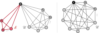
We construct graphs as hard instances for estimating . In graph , the target node has neighbors, which can be divided into groups. Each of the first groups, denoted by for , has neighbor nodes, while the last group, denoted by , contains neighbors. In the first groups, each neighbor node has a degree of , whereas in the -th group, each neighbor node has a degree of . Additionally, we add isolated nodes to these graphs, ensuring that the number of nodes in each graph is . Figure 1 illustrates graphs and .
We denote the PageRank score of in graph as . We will demonstrate that for each ,
Specifically, in graph , each node belonging to group for has a Personalized PageRank (PPR) score . Furthermore, each node in graph has a PPR score . Additionally, the PPR score of node to itself is . Thus, according to Equation (5), the PageRank score of node in graph is
The difference , which corroborates the assertion that for each .
Furthermore, let represent the set of all graphs that are isomorphic to obtained through permutation of node labels. Consider an undirected graph , chosen uniformly at random from . Any algorithm is required to identify the specific set from which originates. Failing this, the probability that can estimate within a multiplicative factor of diminishes to at most , a result deemed unacceptable.
Finally, in the arc-centric graph access model, we contend that any algorithm must execute queries in expectation to distinguish between graphs and for any . By our design, must detect at least one node in group to discern the difference between graphs and , given that other sections of the two graphs remain indistinguishable. It is important to note that can explore unseen nodes in the underlying graph only through interactions with the graph oracle, utilizing the three elementary query operations: , , and . When employing the query, is expected to perform jump queries to detect a node in group with probability at least . However, this complexity, , exceeds the stated lower bound asymptotically. Consequently, the viable strategy for is only local access through and queries. This approach requires to perform queries on average to detect at least one node in . Notably, , given that holds in these hard instances. This substantiates the proposed lower bound of , thus concluding the proof. ∎
6. Experiments
We evaluate our BackMC algorithm against other baseline methods on large-scale real-world and synthetic graphs.
| Dataset | Graph Type | |||
| Youtube(YT) | Real-World | 1,138,499 | 5,980,886 | 1 |
| LiveJournal (LJ) | Real-World | 4,847,571 | 85,702,474 | 1 |
| Twitter (TW) | Real-World | 41,652,230 | 2,405,026,092 | 1 |
| Friendster (FR) | Real-World | 68,349,466 | 3,623,698,684 | 1 |
| ER10 | Synthetic | 100,000 | 1,001,008 | 1 |
| ER100 | Synthetic | 100,000 | 9,993,692 | 59 |
| ER1000 | Synthetic | 100,000 | 100,001,498 | 875 |
| ER10000 | Synthetic | 100,000 | 1,000,052,806 | 9582 |
Environment. We conduct all the experiments on a Linux server with an Intel (R) Xeon(R) Gold 6126@2.60GHz CPU and 500GB memory. All the methods are implemented in C++ and compiled in g++ with the O3 optimization turned on.
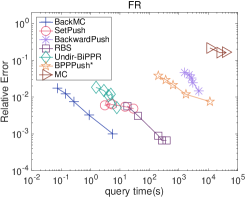
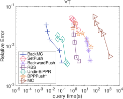
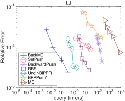
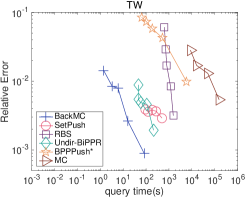
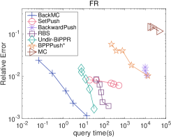
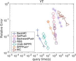
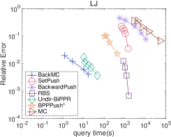
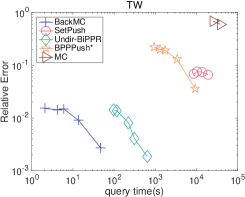
Methods and Parameters. We compare our BackMC against six baseline methods, including MC (fogaras2005MC, ), BackwardPush (lofgren2013personalized, ), RBS (wang2020RBS, ), SetPush (setpush2023VLDB, ), Undir-BiPPR 333It’s worth noting that Undir-BiPPR (lofgren2015bidirectional_undirected, ) is initially implemented as a combination of forward push and MC, which however is impractical under the graph access model due to the time required to identify all nodes for pushing in the initial state. Instead, we implement Undir-BiPPR by combining backward push and MC, ensuring an complexity under the graph access model. (lofgren2015bidirectional_undirected, ), and (bressan2023sublinear, ). Additionally, we compute the ground truths by iteratively updating the PageRank vector using Equation (1). Initially, we set and repeat the iteration times. Then for any given target node , we utilize the derived as the ground truth of the PageRank score of . Throughout our experiments, we set the failure probability to and vary the relative error within the range to analyze the tradeoff between query time and actual Relative Error (as defined below) for each method. Moreover, unless otherwise specified, we set the teleport probability to .
Metrics. We consider actual Relative Error, which is defined as
On each dataset, we sample nodes as the target node , and execute each method once for each target node. Subsequently, we compute the average actual Relative Error of each method for estimating across all query nodes under each setting of .
|
|
|
|
|
|
|
|
|
|
|
|
6.1. Experiments on Real-World Graphs
We first evaluate our BackMC against other baseline methods on large-scale real-world graphs.
Datasets. We utilize four real-world datasets in our experiments: YouTube (YT), LiveJournal (LJ), Twitter (TW), and Friendster (FR). These datasets originate from social networks and are publicly available 444http://law.di.unimi.it/datasets.php 555http://snap.stanford.edu/data. In these graphs, nodes represent users on the respective websites, and edges denote friendships between users. Table 3 presents the statistics of the four datasets.
Target Nodes. For each dataset, we sample two subsets from the node set of , each containing nodes designated as target nodes. In the first subset, nodes are randomly selected from with a uniform distribution. In contrast, nodes in the second subset are chosen from based on the degree distribution. Specifically, for any node , the likelihood of being sampled in the second subset increases with its degree . This sampling strategy allows us to evaluate the performance of all methods in estimating for nodes with high degrees.
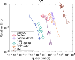
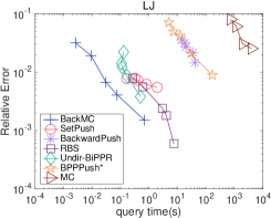
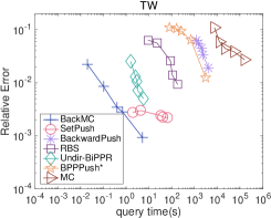
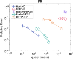
Results. Figure 4 shows the tradeoffs between query time and actual Relative Error for each method, with the target node uniformly selected from . We note that BackMC consistently achieves the shortest query time compared to the other baseline methods at the same actual Relative Error level. Specifically, BackMC outperforms Undir-BiPPR, SetPush, and RBS by a factor of , and surpasses , MC, and BackwardPush by to , in general. Particularly noteworthy is the significant superiority of BackMC over SetPush, which previously established the best complexity bound for estimating . This empirical observation aligns with our theoretical arguments, not only showcasing the theoretical improvement of BackMC over SetPush but also highlighting the clean algorithm structure and ease of implementation. Additionally, as mentioned in Section 4.2, the presence of a multiplicative factor in the complexity bound of SetPush hampers its empirical performance efficiency.
Figure 4 illustrates the tradeoffs between query time and actual Relative Error for each method, with the target node sampled from the degree distribution. Analogously, BackMC consistently outperforms all baseline methods on all datasets in terms of both efficiency and accuracy. Notably, we omit the BackwardPush method from the Twitter dataset analysis due to its query time exceeding 12 hours. This observation aligns with our analysis that considerable time is required by BackwardPush to perform push operations on nodes with high degrees, given that the Twitter dataset is dense with a large average degree, as shown in Table 3.
In Figures 4 and 4, we maintain a fixed teleport probability of 0.2. In Figure 4, we present the tradeoffs between query time and actual Relative Error with . Target nodes are uniformly sampled from . Comparing the results from Figure 4 and Figure 4, we observe a more pronounced superiority of BackMC over SetPush. This aligns well with our analysis that the SetPush method has a multiplicative factor of in its complexity bound, which will become significant when is small. In contrast, the computational complexity of our BackMC has a multiplicative factor, which is more favorable than that of SetPush. Additionally, a small also makes the query time of RBS unaffordable on large-scale Twitter and Friendster datasets. We omit them from Figure 4. We also exclude BackwardPush on Twitter and MC on Friendster from Figure 4, as their query time both exceed 12h.
6.2. Experiments on Synthetic Graphs
In this subsection, we evaluate BackMC and the competitors on synthetic Erdős–Rényi (ER) graphs.
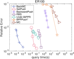
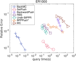
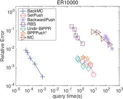
Datasets. We generate four ER graphs, each comprising a fixed number of nodes (). The first graph, designated as ER10, features an edge-connection probability of between any two nodes. In other words, the probability that any given pair of nodes in the ER10 graph will be connected is consistently set to . This connection probability is sequentially increased to , , and for the subsequent graphs, referred to as ER100, ER1000, and ER10000, respectively. As a direct outcome, the average degree of nodes in the ER10 graph is approximately , while the corresponding average degrees in the ER100, ER1000, and ER10000 graphs are roughly , , and , respectively. Notably, we present the minimum degree (i.e., ) observed in these four ER graphs in Table 3, which are around , , , and for each graph, in ascending order of connection probability. These variations in ER graphs serve as a basis to demonstrate the superior performance of BackMC across a spectrum of graphs distinguished by differing values of .

|
|
|
|
Results. In Figure 5, we present the trade-off between actual relative error and query time across the four ER graphs. Our first observation is that BackMC consistently surpasses all baseline methods by orders of magnitude in query time for the same level of actual relative error. Notably, the margin of BackMC’s superiority over its competitors increases as rises. Specifically, on the ER10 graph, BackMC is tenfold faster than both SetPush, Undir-BiPPR and RBS. This leading factor escalates from tenfold to a thousandfold. On the ER10000 graph, BackMC exceeds the performance of all competitors by at least three orders of magnitude in query time for comparable actual relative errors. Additionally, it is important to highlight that while the query time for competitor methods escalates with an increase in (thus attributable to the growing number of edges), BackMC uniquely exhibits reduced query times as increases. This phenomenon underscores BackMC’s exceptional efficiency and corroborates our analysis, demonstrating a negative correlation between the computational complexity of BackMC and .
7. Conclusion
This paper introduces a simple and optimal algorithm, BackMC, for estimating a single node’s PageRank score in undirected graphs. We have demonstrated the optimality of BackMC and assessed its performance on large-scale graphs. As for future directions, we aim to adapt BackMC to tackle single-pair PPR queries in undirected graphs. Given that the computation of PPR scores relates closely to that of PageRank scores, as shown in Equation (5), we are motivated to investigate further in this area.
Acknowledgements.
I would like to thank Professor Zhewei Wei for his unconditional support. I would also like to thank the anonymous reviewers for their insightful comments.References
- [1] Reid Andersen, Christian Borgs, Jennifer Chayes, John Hopcraft, Vahab S Mirrokni, and Shang-Hua Teng. Local computation of pagerank contributions. In International Workshop on Algorithms and Models for the Web-Graph, pages 150–165. Springer, 2007.
- [2] Konstantin Avrachenkov, Nelly Litvak, Danil Nemirovsky, and Natalia Osipova. Monte carlo methods in pagerank computation: When one iteration is sufficient. SIAM Journal on Numerical Analysis, 45(2):890–904, 2007.
- [3] Ziv Bar-Yossef and Li-Tal Mashiach. Local approximation of pagerank and reverse pagerank. In Proceedings of the 17th ACM conference on Information and knowledge management, pages 279–288, 2008.
- [4] Aleksandar Bojchevski, Johannes Klicpera, Bryan Perozzi, Amol Kapoor, Martin Blais, Benedek Rózemberczki, Michal Lukasik, and Stephan Günnemann. Scaling graph neural networks with approximate pagerank. In Proceedings of the 26th ACM SIGKDD International Conference on Knowledge Discovery and Data Mining, New York, NY, USA, 2020. ACM.
- [5] Christian Borgs, Michael Brautbar, Jennifer Chayes, and Shang-Hua Teng. A sublinear time algorithm for pagerank computations. In International Workshop on Algorithms and Models for the Web-Graph, pages 41–53. Springer, 2012.
- [6] Christian Borgs, Michael Brautbar, Jennifer Chayes, and Shang-Hua Teng. Multiscale matrix sampling and sublinear-time pagerank computation. Internet Mathematics, 10(1-2):20–48, 2014.
- [7] Marco Bressan, Enoch Peserico, and Luca Pretto. Sublinear algorithms for local graph centrality estimation. In 2018 IEEE 59th Annual Symposium on Foundations of Computer Science (FOCS), pages 709–718. IEEE, 2018.
- [8] Marco Bressan, Enoch Peserico, and Luca Pretto. Sublinear algorithms for local graph-centrality estimation. SIAM Journal on Computing, 52(4):968–1008, 2023.
- [9] Sergey Brin and Lawrence Page. The anatomy of a large-scale hypertextual web search engine. Computer networks and ISDN systems, 30(1-7):107–117, 1998.
- [10] Ming Chen, Zhewei Wei, Bolin Ding, Yaliang Li, Ye Yuan, Xiaoyong Du, and Ji-Rong Wen. Scalable graph neural networks via bidirectional propagation. arXiv preprint arXiv:2010.15421, 2020.
- [11] Yen-Yu Chen, Qingqing Gan, and Torsten Suel. Local methods for estimating pagerank values. In Proceedings of the thirteenth ACM international conference on Information and knowledge management, pages 381–389, 2004.
- [12] Paul Dagum, Richard Karp, Michael Luby, and Sheldon Ross. An optimal algorithm for monte carlo estimation. SIAM Journal on computing, 29(5):1484–1496, 2000.
- [13] Dániel Fogaras, Balázs Rácz, Károly Csalogány, and Tamás Sarlós. Towards scaling fully personalized pagerank: Algorithms, lower bounds, and experiments. Internet Mathematics, 2(3):333–358, 2005.
- [14] David F Gleich. Pagerank beyond the web. siam REVIEW, 57(3):321–363, 2015.
- [15] Goldreich and Ron. Property testing in bounded degree graphs. Algorithmica, 32(2):302–343, 2002.
- [16] Oded Goldreich, Shari Goldwasser, and Dana Ron. Property testing and its connection to learning and approximation. Journal of the ACM (JACM), 45(4):653–750, 1998.
- [17] Marco Gori, Augusto Pucci, Via Roma, and I Siena. Itemrank: A random-walk based scoring algorithm for recommender engines. In IJCAI, volume 7, pages 2766–2771, 2007.
- [18] Vince Grolmusz. A note on the pagerank of undirected graphs. Information Processing Letters, 115(6-8):633–634, 2015.
- [19] Pankaj Gupta, Ashish Goel, Jimmy Lin, Aneesh Sharma, Dong Wang, and Reza Zadeh. Wtf: The who to follow service at twitter. In Proceedings of the 22nd international conference on World Wide Web, pages 505–514, 2013.
- [20] Zoltán Gyöngyi, Hector Garcia-Molina, and Jan Pedersen. Combating web spam with trustrank. In Proceedings of the Thirtieth international conference on Very large data bases-Volume 30, pages 576–587, 2004.
- [21] Johannes Klicpera, Aleksandar Bojchevski, and Stephan Günnemann. Predict then propagate: Graph neural networks meet personalized pagerank. In ICLR, 2019.
- [22] Peter Lofgren, Siddhartha Banerjee, and Ashish Goel. Bidirectional pagerank estimation: From average-case to worst-case. In Algorithms and Models for the Web Graph: 12th International Workshop, WAW 2015, Eindhoven, The Netherlands, December 10-11, 2015, Proceedings 12, pages 164–176. Springer, 2015.
- [23] Peter Lofgren, Siddhartha Banerjee, and Ashish Goel. Personalized pagerank estimation and search: A bidirectional approach. In Proceedings of the Ninth ACM International Conference on Web Search and Data Mining, pages 163–172, 2016.
- [24] Peter Lofgren and Ashish Goel. Personalized pagerank to a target node. arXiv preprint arXiv:1304.4658, 2013.
- [25] Peter A Lofgren, Siddhartha Banerjee, Ashish Goel, and C Seshadhri. Fast-ppr: Scaling personalized pagerank estimation for large graphs. In Proceedings of the 20th ACM SIGKDD international conference on Knowledge discovery and data mining, pages 1436–1445, 2014.
- [26] Barbara Logan Mooney, L René Corrales, and Aurora E Clark. Molecularnetworks: An integrated graph theoretic and data mining tool to explore solvent organization in molecular simulation. Journal of computational chemistry, 33(8):853–860, 2012.
- [27] Julie L Morrison, Rainer Breitling, Desmond J Higham, and David R Gilbert. Generank: using search engine technology for the analysis of microarray experiments. BMC bioinformatics, 6(1):1–14, 2005.
- [28] Lawrence Page, Sergey Brin, Rajeev Motwani, and Terry Winograd. The pagerank citation ranking: bringing order to the web. 1999.
- [29] Bryan Perozzi, Rami Al-Rfou, and Steven Skiena. Deepwalk: Online learning of social representations. In Proceedings of the 20th ACM SIGKDD international conference on Knowledge discovery and data mining, pages 701–710, 2014.
- [30] Hanzhi Wang, Mingguo He, Zhewei Wei, Sibo Wang, Ye Yuan, Xiaoyong Du, and Ji-Rong Wen. Approximate graph propagation. In Proceedings of the 27th ACM SIGKDD Conference on Knowledge Discovery & Data Mining, pages 1686–1696, 2021.
- [31] Hanzhi Wang and Zhewei Wei. Estimating single-node pagerank in time. Proc. VLDB Endow., 16(11):2949–2961, 2023.
- [32] Hanzhi Wang, Zhewei Wei, Junhao Gan, Sibo Wang, and Zengfeng Huang. Personalized pagerank to a target node, revisited. In Proceedings of the 26th ACM SIGKDD International Conference on Knowledge Discovery & Data Mining, pages 657–667, 2020.
- [33] Hanqing Zeng, Hongkuan Zhou, Ajitesh Srivastava, Rajgopal Kannan, and Viktor Prasanna. GraphSAINT: Graph sampling based inductive learning method. In ICLR, 2020.