Accurate and Fast Estimation of Temporal Motifs using Path Sampling

Abstract

Counting the number of small subgraphs, called motifs, is a fundamental problem in social network analysis and graph mining. Many real-world networks are directed and temporal, where edges have timestamps. Motif counting in directed, temporal graphs is especially challenging because there are a plethora of different kinds of patterns. Temporal motif counts reveal much richer information and there is a need for scalable algorithms for motif counting.

A major challenge in counting is that there can be trillions of temporal motif matches even with a graph with only millions of vertices. Both the motifs and the input graphs can have multiple edges between two vertices, leading to a combinatorial explosion problem. Counting temporal motifs involving just four vertices is not feasible with current state-of-the-art algorithms.

We design an algorithm, TEACUPS, that addresses this problem using a novel technique of temporal path sampling. We combine a path sampling method with carefully designed temporal data structures, to propose an efficient approximate algorithm for temporal motif counting. TEACUPS is an unbiased estimator with provable concentration behavior, which can be used to bound the estimation error. For a Bitcoin graph with hundreds of millions of edges, TEACUPS runs in less than 1 minute, while the exact counting algorithm takes more than a day. We empirically demonstrate the accuracy of TEACUPS on large datasets, showing an average of 30$\times$ speedup (up to 2000$\times$ speedup) compared to existing GPU-based exact counting methods while preserving high count estimation accuracy.

I Introduction

Mining small subgraph patterns, referred to as motifs, is a central problem in network analysis [1]. Motif mining plays a critical role in understanding the structure and function of complex systems encoded as graphs [2, 3, 4]. There is a rich body of work on mining motifs in static graphs [5, 6, 7, 8, 9, 10] (refer to the tutorial [11] for details). Most real-world phenomena representing networks, e.g., social interaction, communication, are dynamic, where edges are created with timestamps. Static graphs are built by omitting crucial temporal information.

Temporal edges between nodes are tuples $(u,v,t)$, where $u$ and $v$ are source and destination nodes, and $t$ is the timestamp of the edge. Edges with timestamps capture richer information compared to static edges [12, 13]. A graph with such temporal edges is called a temporal graph, and patterns in such graphs are called temporal motifs. Temporal motifs are useful in user behavior characterization on social/communication networks [12, 14, 15, 16], detecting fraud in financial transaction networks [17, 18], and characterizing the structure and function of biological networks [13, 19]. Furthermore, local motif counts are useful to resolve symmetries and improve the expressive power of GNNs [20, 18, 21].

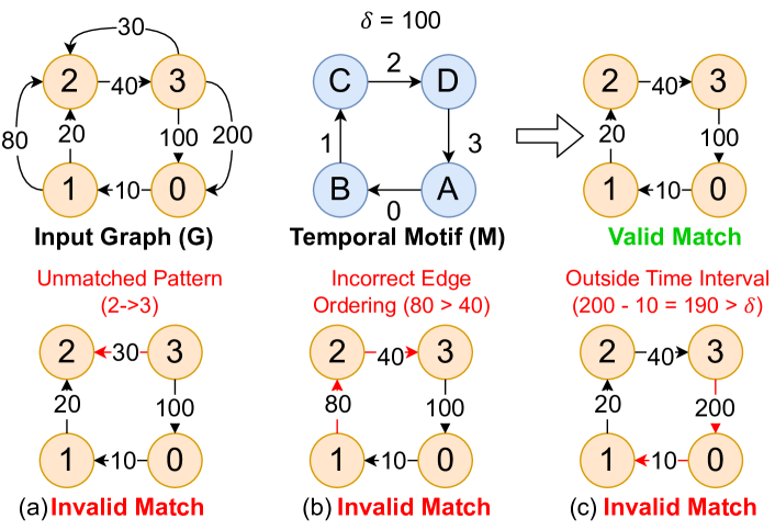
Figure 1: An example of mining a temporal motif (M) from a input graph (G)

I-A Formal Problem Definition

The input is a directed temporal graph $G=(V(G),E(G))$, with $n$ vertices and $m$ edges. Each temporal edge is a tuple $e=(u,v,t)$ where $u$ and $v$ are vertices in the temporal graph, and $t$ is a positive integer timestamp. Note that the graph is directed, and there can be many edges between the same $u$ and $v$. For temporal edge $e$, we use $t(e)$ to denote its timestamp. For convenience, we think of time in seconds.

We formally define a temporal motif and a match, following Paranjape et al. [16]. (Our match definition is non-induced, since we only match edges. This is consistent with past work.)

Definition I.1.

A temporal motif is a triple $M=(H,\pi,\delta)$ where (i) $H=(V(H),E(H))$ is a directed pattern multi-graph, $(ii)$ $\pi$ is a permutation on the edges of $H$, and (iii) $\delta$ is a positive integer.

The permutation $\pi$ specifies the time ordering of edges, and $\delta$ specifies the length of time interval for all edges.

Definition I.2.

Consider an input temporal graph $G=(V(G),E(G))$ and a temporal pattern $M=(H,\pi,\delta)$. An $M$-match is a 1-1 map $\phi:V(H)\to V(G)$ satisfying the following conditions.

• (Matching the pattern) The map $\phi$ matches the edges of $H$. Formally, $\forall(u,v)\in E(H)$, $(\phi(u),\phi(v))\in E(G)$. For convenience, for edge $e\in E(H)$, we use $\phi(e)$ to denote the match in the pattern.

• (Edges ordered correctly) The timestamps of the edges in the match follow the ordering $\pi$. Formally, $\forall e,e^{\prime}\in E(H)$, $\pi(e)<\pi(e^{\prime})$ iff $t(\phi(e))<t(\phi(e^{\prime}))$.

• (Edges in time interval) All edges of the match occur within $\delta$ time. $\forall e,e^{\prime}\in E(H)$, $|t(\phi(e))-t(\phi(e^{\prime}))|\leq\delta$.

TABLE I: Summary of notation

Symbol	Definition
$\delta$	maximum time window
$M=(H,\pi,\delta)$	a directed temporal motif with $\delta$ time window
$G=(V(G),H(G))$	a directed temporal graph
$S$	the wedge or 3-path chosen from $M$
$P$	the sampled wedge or 3-path from $G$ that maps to $S$
$w_{e,\delta}$	the sampling weight of edge $e$ in $G$
$W_{\delta}$	the total number of $\delta$-centered wedge or 3-path

For convenience, we summarize the symbols and definitions in Table I. Some symbols are defined later.

As a walkthrough example in Figure 1, we want to mine a temporal motif $M$ with $\delta=100$ from an input graph $G$. We show one valid match and three invalid matches. Those matches are invalid due to: (a) the edge direction between nodes 2 and 3 is opposite to the pattern in M; (b) edge (1, 2, 80) occurs after edge (2, 3, 40), which violates the edge ordering constraints in M; (c) the edge (3, 0, 200) happens 190 seconds after the first edge (0, 1, 10), exceeding the maximum time window $\delta$.

In Figure 2, we show 3- and 4-vertex temporal motifs. In our definition, we also allow multiple edges between two vertices. For example, pattern $M_{4-4}$ involves 10 edges. Every pair of vertices has 2 edges. A match needs to find 10 edges satisfying the edge pattern, directions, and timestamp orderings.

(a) $M_{\text{3-0}}$

(b) $M_{\text{3-1}}$

(c) $M_{\text{4-0}}$

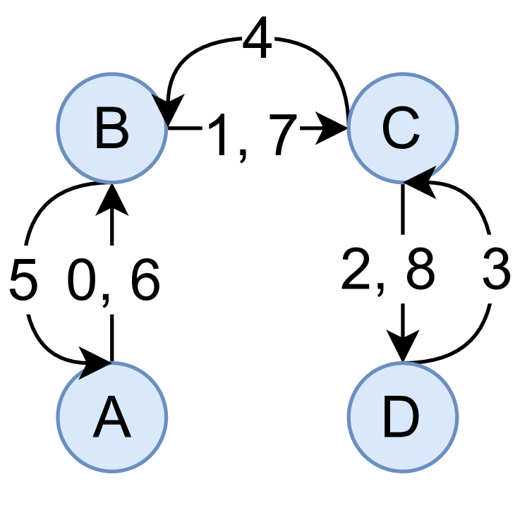
(d) $M_{\text{4-1}}$

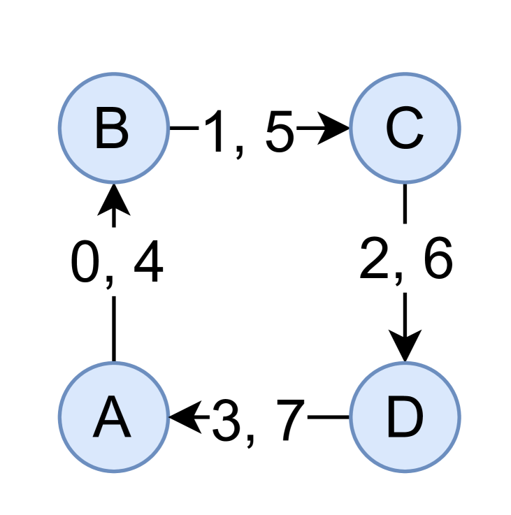
(e) $M_{\text{4-2}}$

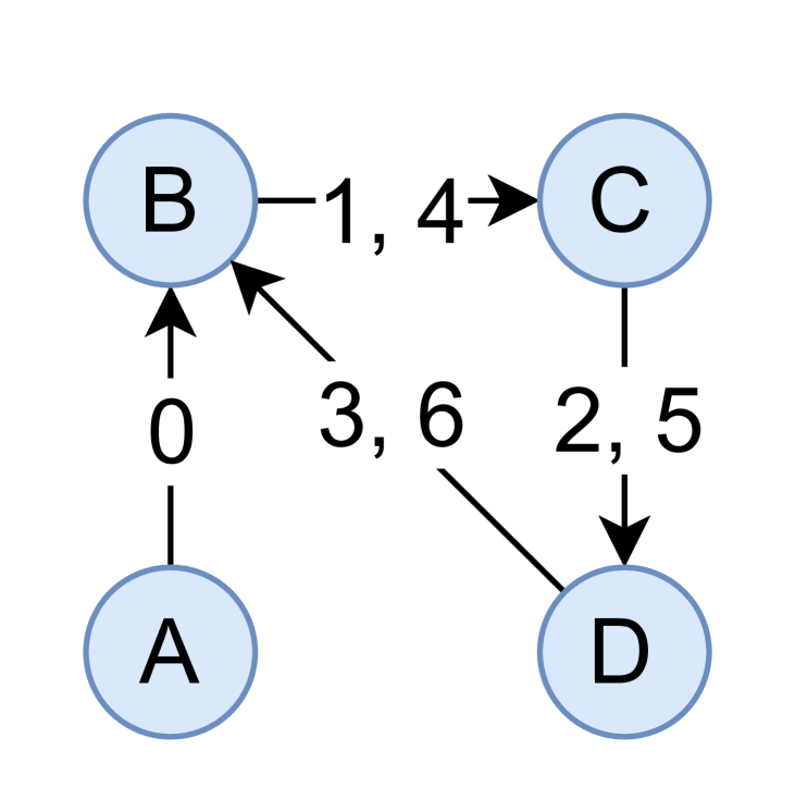
(f) $M_{\text{4-3}}$

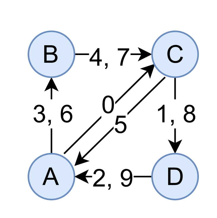
(g) $M_{\text{4-4}}$

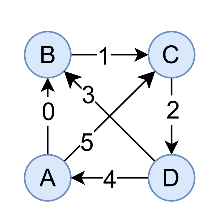
(h) $M_{\text{4-5}}$

Figure 2: A subset of connected temporal motifs.

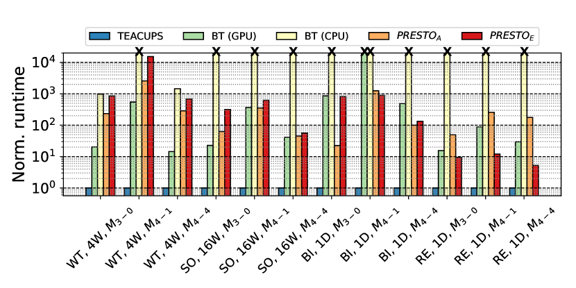
(a) Runtime of prior works normalized to TEACUPS(ours). TEACUPS has up to 1e4$\times$ speedup compared to previous works.

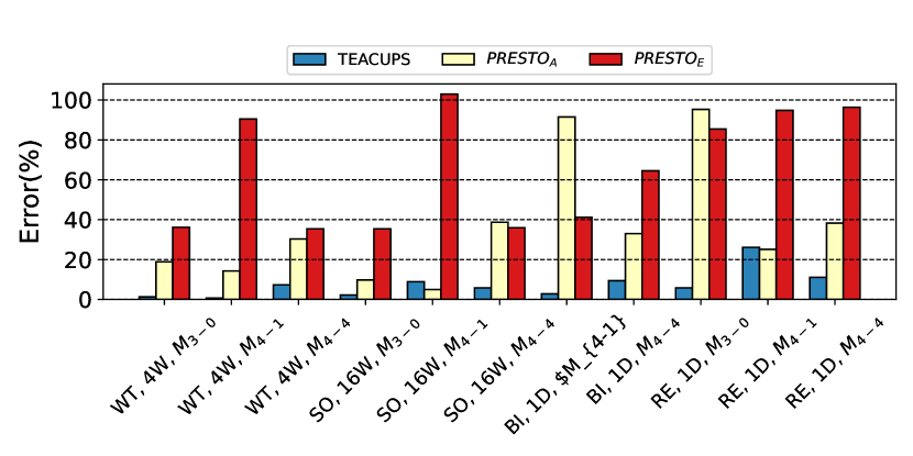
(b) Relative error (%) of approximate algorithms. TEACUPS(ours) is almost always the most accurate while always the fastest. The errors for (BI, 1D, $M_{\text{3-1}}$) are missing because the exact count is unavailable (Everest GPU cannot finish in 1 day).

Figure 3: Normalized runtime of exact algorithms (Everest GPU and BT CPU) and approximate algorithms (TEACUPS, $PRESTO_{A}$, and $PRESTO_{B}$) on various datasets, time ranges and motifs. Except Everst (GPU) which runs on an NVIDIA A40 GPU, all other experiments run on CPU with 32 threads.

I-B Challenges in Mining Temporal Motifs

There are two major challenges where temporal motif counting distinguishes itself from static versions. First, a temporal motif involves ordering relations between the timestamps of edges. For example, Figure 1(b) shows an invalid match because of violating the edge ordering constraints. Most of the best static motif counting techniques exploit motif structure and static graph properties like degeneracy [22, 7, 10, 11]. These specific techniques do not work when imposing ordering constraints on edges. Currently, the best results for temporal motif counting are only practical for simple temporal triangles (3-vertex motifs) [16, 23, 24]. No current method can get 4-vertex motif count results for the Bitcoin graph (100M temporal edges) even within one day on commodity GPU platform.

Second challenge is the combinatorial explosion problem due to multi-graphs (both the input graph and motif). In input graphs, there can be thousands of temporal edges between the same pair of edges. (A static directed graph only has two possible edges.) The edge multiplicity of the input graph itself already causes a large amount of search space and the number of matched instances. For Bitcoin graph with 110 million edges, there are trillion copies of a simple temporal 4-cycle ($M_{\text{4-0}}$). However, the introduction of multi-graph motifs further compounds this explosion, making the search space for temporal multi-graph motifs orders of magnitude larger than their simpler counterparts. The number of instances of temporal multi-graph 4-cycle ($M_{\text{4-2}}$) in the Bitcoin input graph reaches hundreds of trillion, two orders of magnitude larger than the simple 4-cycle. Methods based on enumeration or exploration, no matter how well designed, cannot avoid this massive computation [16, 25].

To summarize, there are numerous temporal patterns (like Figure 2) involving just 3- and 4-vertices, so we cannot hope to define specialized algorithms for motifs. At the same time, general methods are often based on neighborhood exploration that suffer a massive computational explosion because of temporal edge multiplicity.

This motivates the central question behind this work: How can we design scalable algorithms for temporal motif counting that can go beyond triangles and extend to patterns with multiple parallel edges between any pair of vertices?

To address these challenges, this work presents the first scalable algorithm for counting temporal patterns involving up to four vertices and any number of edges in large networks. While the best prior algorithms only work for patterns with up to three vertices [22, 7, 10, 11], we take a major step forward to support complex pattern matching use-cases. An extension of our algorithm to count motifs with more than four vertices involves generalizing path sampling techniques to spanning trees, which is out of the scope of this paper, and is left for future work.

I-C Main Contributions

In this paper, we design the Temporal Explorations Accurately Counted Using Path Sampling algorithm, called TEACUPS. TEACUPS is a fast and accurate. Below, we summarize our contributions.

The Concept of Sampling Temporal Paths. Our main conceptual contribution is the introduction of temporal path sampling. Many of the best static motif counting methods use path or tree sampling [22, 6, 8, 26]. We show how to generalize the method of wedge or $3$-path sampling for temporal graphs. There are significant challenges since direction and temporal orderings create many different kinds of wedges/$3$-paths for a single static wedge/$3$-path. We couple the randomized sampling methods with carefully designed temporal data structures. This leads to an all-purpose temporal sampler, that can sample paths with any ordering and time interval constraints. Based on this sampler, we design the TEACUPS algorithm. All temporal motifs on $4$ vertices contain a temporal $3$-path, and all 3-vertex motifs contain a temporal wedge. TEACUPS is a randomized algorithm that can be applied to all such motifs to estimate motif counts.

In the static case [22], there is an easy way to extend the sampled 3-path into an instance of the motif by checking if the edge exists. However, this does not work for temporal motif counting due to multi-graph. We present an efficient algorithm, which determines the number of instances of the target motif induced by the sampled 3-path in time, linear in the multiplicity of the edges.

Counting Temporal Multi-Graph Motifs. In extending motif patterns to encompass multi-graphs, we uncover more intricate transactional or communicational features in real-world scenarios. Although input graphs often take the form of multi-graphs, prior research has largely neglected motifs within this context. Existing general algorithms [16, 25] show diminished efficiency in this domain, while algorithms designed for rapid processing  [22, 23, 24] are ineffectual for temporal multi-graph motif counting. To the best of our knowledge, this is the first work that specifically focuses on motif patterns that are multi-graphs.

Provable Correctness with Bounded Error. TEACUPS always gives unbiased estimates. Additionally, we rigorously bound the approximation error using techniques from randomized algorithms. We apply concentration inequalities to prove that TEACUPS accurately estimates to temporal motif counts.

Scalable Runtime. We perform an empirical analysis of TEACUPS on numerous real-world temporal datasets. TEACUPS is extremely fast. Figure 3(a) shows the highlight of runtime for the state-of-the-art algorithms (exact and approximate). We give results for numerous datasets and time windows. Across all experiments, TEACUPS is $10$-$1000\times$ faster than existing works. For example, TEACUPS takes less than 1 minute on a Bitcoin graph with 110M edges, where the motif count is over a trillion. The exact count algorithm takes more than one day, and approximate methods either have high error rates or are at least $10\times$ slower. Even compared to the exact count algorithm that runs on an NVIDIA GPU, our algorithm that runs on a CPU exhibits an average of 30$\times$ speedup. Additionally, TEACUPS exhibits a near-linear runtime scalability with CPU threads.

Empirical Accuracy. We empirically validate TEACUPS on a variety of datasets and conduct convergence experiments. TEACUPS consistently achieves a relative error of $<10\%$ for the majority of motifs. In all cases, TEACUPS has a lower or comparable error to existing sampling methods, while being at least 10$\times$ faster, as shown in Figure 3(b).

II Related Work

Static Motif Mining. There are various works on mining static motifs, including the exact count or enumeration methods [27, 28, 29, 30, 31, 32, 33, 34, 35], and approximate techniques [36, 22, 6, 37, 38, 39, 40, 26, 41, 8, 42, 43, 44, 45, 46]. Although static motif mining can serve as a first step for temporal motif mining [16], it is shown that it causes orders of magnitude redundant work, which calls for efficient algorithms tailored to the temporal motif mining problem.

Exact Temporal Motif Counting. The problem of temporal motif mining is first formally described by Paranjape et al. [16], where they propose an algorithm to enumerate and count the temporal motif instances. A more recent exact counting algorithm [25] proposed a backtracking algorithm by enumerating all instances on chronologically sorted edges. Everest [47] supports the backtracking exact counting algorithm on GPUs with system-level optimizations that improve performance by an order of magnitude. There are other general temporal motif count algorithms [48, 49]. A critical challenge with the exact counting algorithms is scalability with respect to graph and motif sizes as enumeration all possible matches takes a large portion of memory and compute resources. A few algorithms focus on mining specific motifs [50, 23, 24, 51]. These solutions, however, are limited to simpler motifs and do not address multi-graph motifs.

Approximate Temporal Motif Counting. To address the scalability issue, Interval-Sampling [37] proposed a sampling algorithm by partitioning times into intervals. PRESTO [52] improved the sampling method by leveraging uniform sampling based on Liu et al. [37]. Edge-Sampling [38] estimates the total number of temporal motifs by exactly counting the local motifs from uniformly sampled temporal edges. Additionally, an online, single-pass sampling algorithm was developed by Ahmed et al. [53]. These approaches, however, have two drawbacks. First, they use uniform sampling while the input graphs are skewed, affecting the accuracy of estimates. Second, their dependency on exact backtracking count algorithm [25] on processing sampled edge subsets necessitates examining every instance, reducing their efficiency.

III Temporal 3-path Sampling

We first define the specific class of temporal $3$-paths that we sample from. Recall that edges of the input graph $G=(V,E)$ are tuples of the form $(u,v,t)$ where $u$ and $v$ are vertices, and $t$ is a timestamp (in seconds). They are sorted by timestamp.

We introduce several crucial definitions, focusing on the concepts of $\delta$-centered wedges and $\delta$-centered 3-paths. In this work, our focus is on using $\delta$-centered 3-paths to obtain accurate estimates of motif-counts for patterns on 4 vertices. This is primarily because counting motifs on 4-vertices is more challenging than triangles, and all of the ideas presented for this setting can be easily generalized to patterns involving 3 vertices.

Definition III.1.

A $\delta$-centered wedge is a pair of edges $e_{1},e_{2}$ with the following properties. Let $e_{1}=(u,v,t(e_{1}))$. Then, $e_{2}$ is incident to $v$. Furthermore, $|t(e_{1})-t(e_{2})|\leq\delta$. We call $e_{1}$ the ”base” edge.

Next, we introduce the notion of a $\delta$-centered $3$-path.

Definition III.2.

A $\delta$-centered $3$-path is a sequence of three edges $e_{1},e_{2},e_{3}$ with the following properties. Let $e_{2}=(u,v,t(e_{2}))$. Then, $e_{1}$ is incident to $u$ and $e_{3}$ is incident to $v$. Furthermore, $|t(e_{1})-t(e_{2})|\leq\delta$ and $|t(e_{3})-t(e_{2})|\leq\delta$.

In particular, a $\delta$-centered $3$-path is a sequence of three ”connected” edges with both end edges within time $\delta$ of the center edge. Our key observation is that such temporal $3$-paths can be sampled rapidly.

A few things to note. There is no $\delta$ constraint between $t(e_{1})$ and $t(e_{3})$. Also, we allow $e_{1}$ and $e_{3}$ to potentially intersect (at a vertex), and even allow $e_{1}$ and $e_{3}$ to contain both $u$ and $v$. Technically, this forms a homomorphism of a $3$-path. We choose the definition above for easy sampling while maintaining some temporal constraints.

We introduce a further categorization of temporal $3$-paths, into 16 classes indexed by 4-bit binary tuples. Specifically, our classes are denoted $\langle\alpha_{1},\alpha_{3},\beta_{1},\beta_{3}\rangle$, where $\alpha_{1},\alpha_{3}\in\{+,-\}$ and $\beta_{1},\beta_{3}\in\{<,>\}$. $\alpha_{i},\beta_{i}$ represent a constraint on the edge $e_{i}$ of a $\delta$-centered $3$-path.

Instead of giving a general definition for all classes, we define the $\langle-,+,<,>\rangle$ class. All other classes are defined analogously.

Definition III.3.

The class of $\langle-,+,<,>\rangle$ $\delta$-centered $3$-paths contains all paths of the following form. Let $(e_{1},e_{2},e_{3})$ be a $\delta$-centered $3$-path and $e_{2}=(u,v,t)$ be the center edge. Then $e_{1}$ is an inedge ($-$) of $u$ and $e_{3}$ is an outedge ($+$) of $v$. Also, $t(e_{1})<t(e_{2})$ and $t(e_{3})>t(e_{2})$.

We stress that there is no condition between $e_{1}$ and $e_{3}$. Note that we can define $\langle+,+,<,<\rangle$ classes and so forth.

We introduce a key definition of multiplicity that are required to express runtime bounds.

Definition III.4.

Given two vertices $u,v$ and timestamps $t<t^{\prime}$, the multiplicity $\sigma_{u,v}[t,t^{\prime}]$ is the number of edges $(u,v,t^{\prime\prime})$ such that $t^{\prime\prime}\in[t,t^{\prime}]$. We denote the maximum $\delta$-multiplicity as $\sigma_{\delta}$, defined as $\max_{u,v,t}$ $\sigma_{u,v}[t,t+\delta]$.

The principle idea behind TEACUPS is to accurately estimate the number of connected 3- or 4-vertex temporal motifs by sampling a subset of temporal wedges or 3-paths, whose edges must satisfy certain temporal constraints, and then determine the motif counts. The algorithm comprises three primary phases: 1) preprocessing to get sampling weights, 2) sampling wedges/3-paths, and 3) deriving desired motif counts from the sampled wedges/3-paths. As mentioned before, in this work, we will focus on 3-path sampling and how it can be used to derive motif counts for connected 4-vertex patterns.

We describe the procedures in the following sections. For convenience, the graph $G=(V,E)$ is assumed to be a global variable accessible to all procedures.

III-A Preprocessing and Sampling Procedure

Our algorithm to estimate the number of connected 4-vertex temporal motifs is primarily based on 3-path sampling. Observe that every 4-vertex motif in Figure 2 contains at least one 3-path. We choose one 3-path as the anchor $S$. Our algorithm and analysis work for all classes of 3-paths. For the sake of readability, we will present the path sampling algorithm for the $\langle-,+,<,>\rangle$ class. All other classes can be sampled analogously.

Our main module is a uniform random sampler for $3$-paths from a specific class. Let’s first set some definitions.

Definition III.5 (Temporal outlists and degrees, $\Lambda^{+}_{v}[t,t^{\prime}]$, $d^{+}_{v}[t,t^{\prime}]$).

Given a vertex $v$ and natural numbers $t,\delta$, the temporal outlist $\Lambda^{+}_{v}[t,t^{\prime}]$ is defined as the set of outedges $(v,w,t^{\prime\prime})$, where $w$ is an arbitrary vertex and $t^{\prime\prime}\in[t,t^{\prime}]$. We similarly define the temporal inlist as $\Lambda^{-}_{v}[t,t^{\prime}]$.

The temporal out-degree $d^{+}_{v}[t,t^{\prime}]$ denotes the size of $\Lambda^{+}_{v}[t,t^{\prime}]$. The temporal in-degree $d^{-}_{v}[t,t^{\prime}]$ is the size of $\Lambda^{-}_{v}[t,t^{\prime}]$.

Definition III.6 ($3$-path counts $w_{e,\delta}$ and $W_{\delta}$).

Fix $\delta$. For a temporal edge $e=(u,v,t)$, $w_{e,\delta}$ denotes the number of $\delta$-centered $\langle-,+,<,>\rangle$ 3-paths, where $e$ is the center edge.

We use $W_{\delta}:=\sum_{e}w_{e,\delta}$ to be the total number of $\delta$-centered $\langle-,+,<,>\rangle$ 3-paths.

The following claim is central to the algorithm and analysis.

Claim III.7.

$w_{e,\delta}=d^{-}_{u}[t-\delta,t]\cdot d^{+}_{v}[t,t+\delta]$.

Proof.

Consider any pair of edges $(x,u,t_{x})$ and $(v,w,t_{w})$ where $x,w$ are arbitrary vertices, $t_{x}\in[t-\delta,t]$ and $t_{w}\in[t,t+\delta]$. Then, these edges form a $\langle+,-,<,>\rangle$ $\delta$-centered $3$-path with $e$ at the center. The number of edges $(x,u,t_{x})$ where $t_{x}\in[t-\delta,t]$ is precisely the indegree $d^{-}_{u}[t-\delta,t]$. Similarly, the number of edges $(v,w,t_{w})$ where $t_{w}\in[t,t+\delta]$ is the outdegree $d^{+}_{v}[t,t+\delta]$. The product of these degrees gives the total number of desired $3$-paths, which is $d^{-}_{u}[t-\delta,t]\cdot d^{+}_{v}[t,t+\delta]$. ∎

Note that we can count $\langle\alpha,\alpha^{\prime},<,>\rangle$ 3-paths with the formula $d^{\alpha}_{u}[t-\delta,t]\cdot d^{\alpha^{\prime}}_{v}[t,t+\delta]$. (To change the $<,>$ indicators in the class, we would focus on different time interval.)

We now describe the actual procedure that samples temporal $3$-paths. We assume that the graph $G$ is stored as an adjacency list of out-edges and in-edges, where each list is sorted by timestamp. So we can perform binary search by time among the edges incident to a vertex. After we select a 3-path $S$ from the motif $M$, we do the following two procedures.

Algorithm 1 : Preprocess($\delta$)

Input: Time $\delta$ (code assumes $\langle-,+,<,>\rangle$ class)

Output: Sampling probability $p_{e,\delta}$ for each edge $e\in E$, and the total sampling weight $W_{\delta}$.

1:for $v\in V$ do

2:     In the in-neighbor list of $v$, binary search for the times $t-\delta$ and $t$. Store the difference in indices to be $d^{-}_{v}[t-\delta,t]$.

3:     In the out-neighbor list of $v$, binary search for the times $t$ and $t+\delta$. Store the difference in indices to be $d^{+}_{v}[t,t+\delta]$.

4:$W_{\delta}=0$

5:for $e=(u,v,t)\in E$ do

6:     $w_{e,\delta}=d^{-}_{u}[t-\delta,t]\cdot d^{+}_{v}[t,t+\delta]$

7:     $W_{\delta}\mathrel{+}=w_{e,\delta}$

8:for $e\in E$ do

9:     $p_{e,\delta}=w_{e,\delta}/W_{\delta}$

First is the Preprocess procedure (Algorithm 1) that constructs a distribution based on $w_{e,\delta}$ values. It crucially uses Claim III.7. The set of values $\{p_{e,\delta}\}$ forms a distribution over the edges. The next procedure, Sample (in Algorithm 2), computes a random $3$-path based on the distribution constructed in the preprocessing step.

Algorithm 2 : Sample$(\{p_{e,\delta}\},\delta)$

Input: Sampling distribution $\{p_{e,\delta}\}$ from Preprocess, and time $\delta$

Output: Uniform random $\langle-,+,<,>\rangle$ $\delta$-centered $3$-path $P$

1:Pick edge $e=(u,v,t)$ with probability $p_{e,\delta}$.

2:In the in-neighbor list of $u$, binary search for the times $t-\delta$ and $t$ to get $\Lambda^{-}_{u}[t-\delta,t]$.

3:Pick uniform random edge $e_{1}$ from $\Lambda^{-}_{u}[t-\delta,t]$.

4:In the out-neighbor list of $v$, binary search for the times $t$ and $t+\delta$ to get $\Lambda^{+}_{v}[t,t+\delta]$.

5:Pick uniform random edge $e_{3}$ from $\Lambda^{+}_{v}[t,t+\delta]$

6:return $P=(e_{1},e,e_{3})$

Claim III.8.

The procedure Preprocess runs in time $O(m\log m)$. The procedure Sample runs in time $O(\log m)$ per sample.

Proof.

We first give the running time of Preprocess. Observe that it performs four binary searches for each edge (two each in the out-neighbors and in-neighbors). The total running time is $O(m\log m)$. $m$ is the number of edges in $G$.

For Sample, the first step is to sample from the distribution given by $\{p_{e,\delta}\}$ values. This can be done using a binary search, which takes $O(\log m)$ time. After that, it performs two binary searches and two random number generations. So the total running time is $O(\log m)$. ∎

Finally, we show that Sample is a bonafide uniform random sampler.

Lemma III.8.1.

The procedure Sample generates a uniform random $\langle-,+,<,>\rangle$ $\delta$-centered $3$-path.

Proof.

Consider a $\langle-,+,<,>\rangle$ $\delta$-centered $3$-path $(e_{1},e_{2},e_{3})$. Let $e_{2}=(u,v,t)$. Then $e_{1}$ is an in-edge of $u$ with timestamp in $[t-\delta,t]$. Also, $e_{3}$ is an out-edge of $v$ with timestamp in $[t,t+\delta]$.

The probability of sampling $e_{2}$ is $w_{e_{2},\delta}/W_{\delta}$. Conditioned on this sample, the probability of sampling $e_{1}$ is precisely $1/|\Lambda^{-}_{u}[t-\delta,t]|$, which is $1/d^{-}_{u}[t-\delta,t]$. Similarly, the probability of sampling $e_{3}$ is $1/d^{+}_{v}[t,t+\delta]$. Multiplying all of these, we get the probability of sampling the entire $3$-path $(e_{1},e_{2},e_{3})$. Applying Claim III.7, the probability is

$$\frac{w_{e_{2},\delta}}{W_{\delta}}\cdot\frac{1}{d^{-}_{u}[t-\delta,t]}\cdot\frac{1}{d^{+}_{v}[t,t+\delta]}$$

$$= \frac{d^{-}_{u}[t-\delta,t]\cdot d^{+}_{v}[t,t+\delta]}{W_{\delta}}\cdot\frac{1}{d^{-}_{u}[t-\delta,t]\cdot d^{+}_{v}[t,t+\delta]}=\frac{1}{W_{\delta}}$$

Hence, the probability of sampling $(e_{1},e_{2},e_{3})$ is $1/W_{\delta}$, which corresponds to the uniform distribution. (By definition, the total number of $\langle-,+,<,>\rangle$ $\delta$-centered $3$-paths is $W_{\delta}$.) ∎

III-B Counting Motifs That Extend a 3-path

The previous section discussed how to sample a 3-path. Once we have a sampled 3-path $P$, we need to determine if it can be “extended” to count a desired motif. We describe the algorithms formally as the procedures CheckMotif and ListCount in high-level.

We first denote the list of edges $(u,v,t)$ in $G$ as $L_{u,v}$. (No constraints on $t$.) We aim to count the temporal motif $M=(H,\pi,\delta)$, using $M_{\text{4-1}}$ from Figure 2 as an example. To do this, we first select a specific 3-path within the motif, referred to as the anchor $S$. This anchor includes the motif edge with the earliest timestamp, labeled as time order 0. For $M_{4-1}$, we choose the 3-path $S$ consisting of the edges labeled $0,1,2$ (the sequence $(A,B,0),(B,C,1),(C,D,2)$).

Algorithm 3 : CheckMotif$(P,M)$

Input: 3-path $P=\{e_{1},e_{2},e_{3}\}$, where $e_{1}=\{u^{\prime},u,t_{1}\}$, $e_{2}=\{u,v,t_{2}\}$, $e_{3}=\{v,v^{\prime},t_{3}\}$, temporal motif $M=(H,\pi,\delta)$ with a chosen anchor path

Output: Motif count $cnt$

1:if ($\{u^{\prime},u,v,v^{\prime}\}$ not all distinct) or ($t_{3}>t_{1}+\delta$) then

2:     return $0$

3:For every edge $e$ of $M$ that is not on the anchor path, use binary search to find the sublist (in $G$) $E_{f}$ of potential matches.

4:Number these lists as $L_{1},L_{2},\cdots L_{l}$ in the time ordering.

5:return ListCount$(L_{1},L_{2},\cdots L_{l})$

The CheckMotif procedure (in Algorithm 3) takes a sampled 3-path $P$ from $G$ as input and returns the count of temporal motif matches to $M$ where $P$ maps to anchor $S$. CheckMotif first checks if the sampled 3-path $P$ is a valid match to anchor $S$ in $M$. The checks are simple: the 3-path must span 4 vertices, and the edge timestamps should have the right order and be within $\delta$ timesteps.

For motif $M$, There could be many different matches of $M$ that have $P$ mapped to the anchor path. For the example of $M_{\text{4-1}}$, we need to find matches to the edges $(A,B,6)$, $(B,A,5)$, $(B,C,7)$, $(C,B,4)$, $(D,C,3)$ and $(C,D,8)$. The adjacency lists are sorted by time. So, using binary search, we can find a sublist of edges in $G$ matching those edges whose timestamp is within $\delta$ of $P$ and is larger than all timestamps in $P$. Let us denote these sublists as $L_{(A,B)},L_{(B,A)},L_{(B,C)},L_{(C,B)},L_{(D,C)}$ and $L_{(C,D)}$ respectively.

We have a further constraint to satisfy. We need to count the number of tuples of edges $(e_{1},e_{2},e_{3},e_{4},e_{5},e_{6})$ from those sublists that maintain this order. To efficiently count these matches without enumerating all possibilities, we employ a method combining pointer traversals with dynamic programming, as described in Algorithm 4.

Algorithm 4 : ListCount($L_{1},L_{2},\dots,L_{l}$)

Input: $l$ sorted lists $L_{1},L_{2},\dots,L_{l}$

Output: The number of $l$ tuples $(l_{1},l_{2},l_{3},\dots,l_{l})$ for which the following holds : 1) $l_{i}\in L_{i}$ for all $1\leq i\leq l$ and 2) $l_{1}\leq l_{2}\leq\dots\leq l_{k}$

1:init $cnt_{1}=\{1\}\times|L_{1}|$ $\triangleright$ $cnt_{r}$ has the same length as $L_{r}$

2:for $r\in[2,l]$ do

3:     for $i\in[0,|L_{r}|)$ do $\triangleright$ $i$ is the pointer to $L_{r}$

4:         $j=0$ $\triangleright$ $j$ is the pointer to $L_{r-1}$

5:         $cursum=0$

6:         while $j<|L_{r-1}|$ and $L_{r-1}[j]\leq L_{r}[i]$ do

7:              $j\mathrel{+}=1$

8:              $cursum\mathrel{+}=cnt_{r-1}[j]$          

9:         $cnt_{r}[i]=cursum$

10:         delete $cnt_{r-1}$      

11:return $\sum cnt_{r}$

Claim III.9.

Given $l$ sorted lists $L_{1},L_{2},\dots,L_{l}$, ListCount runs in time $O(\sum_{r=1}^{l}|L_{r}|)$, where $|L_{r}|$ is the length of $L_{r}$.

III-C The Overall Estimation Procedure

Algorithm 5 Estimate$(M,k)$

Input: Temporal motif $M=(H,\pi,\delta)$, and sample number $k$

Output: Motif count estimate $\widehat{C}$

1:Choose an anchor 3-path of $M$ that has the smallest timeorder edge. Let the 3-path be of type $\langle\alpha_{1},\alpha_{3},\beta_{1},\beta_{3}\rangle$.

2:$\{p_{e,\delta}\},W_{\delta}=\textsc{Preprocess}(\delta)$ (for $\langle\alpha_{1},\alpha_{3},\beta_{1},\beta_{3}\rangle$ class paths)

3:Initialize $cnt=0$

4:for $i\in[1,k]$ do

5:     $P_{i}=\textsc{Sample}(\{p_{e,\delta}\},\delta)$ (for $\langle\alpha_{1},\alpha_{3},\beta_{1},\beta_{3}\rangle$ class)

6:     $cnt=cnt+\textsc{CheckMotif}(P_{i},M)$

7:return $\widehat{C}=(cnt/k)\cdot W_{\delta}$

We now bring the pieces together with our main procedure Estimate (in Algorithm 5). There are some convenient notations to set up for the proof. We use the random variable $X_{i}$ to denote the output of CheckMotif$(P_{i},M)$, which is the number of motif counts extended from the sampled path $P_{i}$. Observe that each path sample $P_{i}$ is chosen independently, so all the $X_{i}$’s are independent. We stress that while the random variables all depend on the graph, we assume that the graph is fixed. The only randomness is over the sampling of the path (in Sample), and the samples are independent of each other. Hence, the $X_{i}$’s are iid random variables.

Claim III.10.

Let $C$ denote the number of $M$-matches in $G$. Then $\mathbf{E}[\widehat{C}]=C$.

Proof.

Every $M$-match in $G$ has a unique anchor path. Let $\mathcal{P}$ be the set of $\delta$-centered 3-paths, of the class determined by the anchor path. For a path $P\in\mathcal{P}$, let $C_{P}$ be the number of $M$-matches where the path $P$ is the anchor. Since each match contains a single anchor path, $\sum_{P\in\mathcal{P}}C_{P}=C$. Observe that many $C_{P}$ values may be zero.

The output of CheckMotif$(P_{i},M)$ is precisely the number of $M$-matches containing $P_{i}$ as an anchor; thus, $X_{i}=C_{P_{i}}$. Note that $cnt=\sum_{i\leq k}C_{P_{i}}$. By linearity of expectation, $\mathbf{E}[cnt]=\sum_{i\leq k}\mathbf{E}[C_{P_{i}}]$.

By the properties of Sample (Lemma III.8.1), the path $P_{i}$ is a uniform random element of $\mathcal{P}$. Recall (Definition III.6) that $W_{\delta}$ is the total size of $\mathcal{P}$. Hence, $\mathbf{E}[C_{P_{i}}]=\sum_{P\in\mathcal{P}}C_{P}/W_{\delta}=C/W_{\delta}$. So $\mathbf{E}[cnt]=kC/W_{\delta}$.

The final output $\widehat{C}=(cnt/k)\cdot W_{\delta}$, so $\mathbf{E}[\widehat{C}]=(W_{\delta}/k)\cdot\mathbf{E}[cnt]=(W_{\delta}/k)\cdot kC/W_{\delta}=C$. ∎

We now show the concentration behavior of $\widehat{C}$. We will need the multiplicative Chernoff bound stated below.

Theorem III.11.

[Theorem 1.1 of [54]] Let $Y_{1},Y_{2},\ldots,Y_{k}$ be independent random variables in $[0,1]$, and let $Y=\sum_{i\leq k}Y_{i}$. Let $\varepsilon\in(0,1)$. Then,

$$\mathbf{Pr}[|Y-\mathbf{E}[Y]|>\varepsilon\mathbf{E}[Y]]\leq 2\exp(-\varepsilon^{2}\mathbf{E}[Y]/3)$$

Using the Chernoff bound, we prove the following theorem.

Theorem III.12.

Suppose the temporal motif $M$ has $r$ edges that are not in selected wedge or 3-path $S$. ($r=|E(M)|-|V(M)|+1)$. Let the error probability be denoted $\gamma>0$. Let the number of samples $k$ be at least $3\sigma^{r}_{\delta}W_{\delta}\ln(\gamma/2)/(C\varepsilon^{2})$. Then, $\mathbf{Pr}[|\widehat{C}-C|>\varepsilon C]<\gamma$.

Proof.

The random variables $X_{i}$ are potentially larger than $1$, so we can only apply Theorem III.11 after suitable scaling. For any path $P\in\mathcal{P}$, let us bound the maximum value of $C_{P}$, which is the number of $M$-matches where $P$ is the anchor. Observe that the matches are determined the edges other than $P$. Recall the procedure CheckMotif that finds $M$-matches involving $P$. It creates a list for every edge of $M$ that is not on the anchor. Each such list is of the form $E_{x,y}[s,s^{\prime}]$ for some vertices $x,y$ on the path $P$, where $|s-s^{\prime}|\leq\delta$. Hence, the length is at most $\sigma_{\delta}$. The count of triples output by the call to ListCount is at most $\sigma^{r}_{\delta}$.

So the maximum value of any $C_{P}$ (and hence any $X_{i}$) is at most $\sigma^{r}_{\delta}$. Let us denote this upper bound as $B$. The random variables $X_{i}/B$ are in $[0,1]$, and we can apply Theorem III.11 to $Y:=\sum_{i\leq k}X_{i}/B$. So, $\mathbf{Pr}[|Y-\mathbf{E}[Y]|>\varepsilon\mathbf{E}[Y]]\leq 2\exp(-\varepsilon^{2}\mathbf{E}[Y]/3)$.

The events $|Y-\mathbf{E}[Y]|>\varepsilon\mathbf{E}[Y]$ and $|\widehat{C}-C|>\varepsilon C$ are identical. Observe that $\mathbf{E}[Y]=\mathbf{E}[\sum_{i\leq k}X_{i}]/B=(k/B)\cdot C/W_{\delta}$ (by the calculations in Claim III.10). We choose $k\geq 3\sigma^{r}_{\delta}W_{\delta}\ln(\gamma/2)/(C\varepsilon^{2})$. Thus, $\mathbf{Pr}[|X-\mathbf{E}[X]|>\varepsilon\mathbf{E}[X]]$ is at most

$$2\exp(-\varepsilon^{2}\mathbf{E}[Y]/3)$$

$$\leq 2\exp(-(\varepsilon^{2}/3)\cdot 3\sigma^{r}_{\delta}W_{\delta}\ln(\gamma/2)/(C\varepsilon^{2})\cdot(1/B)\cdot(C/W_{\delta}))$$

$$=\gamma.$$

∎

We can interpret the bound above roughly as: if Estimate chooses at least $BW_{\delta}/C$ samples, it is guaranteed to give an accurate estimate. Here, $B$ refers to the maximum number of $M$-matches that share an anchor path $S$. Pessimistically, we upper bound $B$ as $\sigma^{r}_{\delta}$. The worst-case upper bound might be quite poor, but as we discuss in Section V, we argue that $BW_{\delta}/C$ is not large in practice.

Our final theorem bounds the running time of Estimate.

Theorem III.13.

The running time of Estimate is $O(m\log m+k\log m+k\sigma_{\delta}(|E(M)|-|V(M)|)$, where $k$ is the number of samples. The space complexity of Estimate is $O(m|V(M)|+\sigma_{\delta}(|E(M)|-|V(M)|))$.

Proof.

According to Claim III.8, the Preprocess procedure takes $O(m\log m)$ time. And running Sample procedure $k$ times takes $O(k\log m)$. For every sample, CheckMotif calls ListCount subroutine. As proved in Claim III.9, the runtime of this procedure is $O(\sum_{i}|L_{i}|)$. The number of lists $L_{i}$ is the number of edges which are not on the specified anchor path in $M$, which is $|E(M)|-(|V(M)|-1)$. Further, each $|L_{i}|$ is bounded by the maximum edge multiplicity within $\delta$ time window ($\sigma_{\delta}$). Therefore, the total runtime is $O(m\log m+k\log m+k\sigma_{\delta}(|E(M)|-|V(M)|))$

The Preprocess procedure stores the sampling weights for each edge in $G$ that are mapped to the selected wedge or 3-path $S$. The storage for sampling weight is $O(m|V(M)-1|)$. The Sample procedure needs $O(\sigma_{\delta})$ for in-edges and out-edges lists. CheckMotif procedure needs to keep the candidate lists of edges. The space needed is $\sum_{i}|L_{i}|$ where there are $|E(M)|-(|V(M)|-1)$ lists. And the auxiliary counter in ListCount subroutine needs space $max_{i}|L_{i}|$. So the total space complexity is $O(m|V(M)|+\sigma_{\delta}(|E(M)|-|V(M)|))$. ∎

IV Brief Description of Wedge Sampling

We begin by fixing one of the wedges in our motif as an anchor, specifically a $\langle+,>\rangle$ $\delta-$centered wedges. Similar to 3-path sampling, the wedge sampling algorithm begins with a preprocessing phase in which each edge in the input graph is assigned a non-negative weight. This weight, denoted as $w_{e,\delta}$, are calculated by $d^{+}_{u}[t,t+\delta]$ for each edge. And these weights are used to set-up a distribution for edge sampling. During the sampling phase, we select an edge $e=(u,v,t)$ from $G$ with probability proportional to $w_{e,\delta}$. Then we uniformly sample a random edge from $\Lambda_{u}^{+}[t,t+\delta]$ that extends the sampled edge $e$ into a $\langle+,>\rangle$ $\delta-$centered wedge wedge. This method ensures that we sample uniform random wedges. If the sampled wedge matches the anchor wedge, the listCount subroutine is then employed to calculate the number of instances of the motif induced by the sampled wedge.

V Practical considerations

TABLE II: The maximum, average, and standard deviation of $B$ for different temporal motifs when $\delta$=4 weeks. The $B$ value is the number of motifs that share the same anchor path.

Dataset [55]	motif	$B_{max}$	$B_{avg}$	$B_{std}$
WT	$M_{\text{4-0}}$	4.20E2	3.59E0	5.86E0
	$M_{\text{4-5}}$	8.36E4	1.59E2	6.76E+2
SO	$M_{\text{4-0}}$	9.80E1	1.88E0	1.82E0
	$M_{\text{4-5}}$	2.28E3	1.94E1	5.73E1

In this section, we give numerous arguments as to why Estimate works in practice. A summary of the algorithm and mathematical analysis of the previous section is the following. We can get accurate estimates to a temporal motif count $C$ with (roughly) $k=\sigma^{r}_{\delta}W_{\delta}/C$ samples. These are pessimistic bounds, since $\sigma_{\delta}$ is a (large) upper bound used in various proofs. In practice, $\sigma_{\delta}$ is in the thousands.

Let us apply better “heuristic” bounds on the sample size $k$ and the runtime. Going through the proof of Theorem III.12, we set $k=\widetilde{B}W_{\delta}/C$, where $\widetilde{B}$ is a reasonable upper bound on the number of motifs that share the same anchor 3-path. We do not need the exact upper bound, since (for estimation) we can afford to ignore some matches. We would like to capture as many motifs as possible, with a small value of $\widetilde{B}$. For the running time, we see that Theorem III.13 gives a sharper bound that depends on the edge multiplicities of the edges in the match (which is trivially upper bounded by the largest multiplicity). Instead of upper bounding by $\sigma_{\delta}$, we can upper bound by $B_{avg}$, which is the average number of motif matches for a wedge or 3-path.

In all, our heuristic bound for the samples required is $\widetilde{B}W_{\delta}/C$ and the runtime (ignoring near-linear preprocess) is $\widetilde{B}\cdot B_{avg}W_{\delta}/C$. Our algorithm is practical due to two main reasons. First, the $\delta$-centered wedges or 3-paths can be sampled efficiently, because their total count $W_{\delta}$ is small. Second, both $\widetilde{B}$ and $B_{avg}$ are quite small in practice. For simplicity, we only discuss $\delta$-centered 3-path here.

On why $\delta$-centered 3-paths work. A naive strategy for sampling 3-paths is to disregard all temporal constraints on the 3-path during preprocessing. This would default to the static 3-path sampling of [6]. The preprocessing would be fast and sampling would be much quicker. The final MotifCount procedure checks for temporal constraints. But discarding all temporal constraints during preprocessing renders the majority of the sampled 3-paths non-compliant with the specified temporal requirements, leading to only 0.01% hit rate of valid 3-paths. The static 3-path sampler does not work, because the number of samples required is infeasible.

An alternate strategy is to satisfy all temporal constraints ($t(e_{0})<t(e_{1})<t(e_{2})<t(e_{0})+\delta$) during preprocessing. This approach eliminates unnecessary samples due to violating timestamp constraints. But preprocessing and sampling become inefficient. Now there are dependencies among the edges $e_{0}$ and $e_{2}$, so sampling takes more time. On sampling $e_{1}$, we have to first sample $e_{0}$, and then depending on $e_{0}$, set up sampling for $e_{2}$. preprocessing time complexity is now $O(m\sigma_{\delta,avg}log\sigma_{\delta,avg})$, where $\sigma_{\delta,avg}$ is the average multiplicity of an edge within the $\delta$-time window.

The $\delta$-centered 3-paths offer a happy medium, wherein sampling is efficient and the total number of paths ($W_{\delta}$) remains low. We see that $W_{\delta}$ is quite comparable to the actual count $C$. Recall that the sample bound is linear in $W_{\delta}/C$, which in practice is quite small.

The typically low values of $\widetilde{B}$ and $B_{avg}$. In Table II, we see that $B_{avg}$ is typically small and much smaller than the maximum value. This means that the practical runtime bounds are also much smaller than the pessimistic worst-case bound. So the value of $\widetilde{B}$ is quite small, suggesting that the number of samples required in Theorem III.12 is not large.

VI Experiments

TABLE III: Temporal graph datasets used in the evaluation.

Dataset	$V$	$|E_{temporal}|$	$|E_{static}|$	Time span (year)
wiki-talk (WT)	1.1M	7.8M	3.3M	6.36
stackoverflow (SO)	2.6M	63.5M	36.2M	7.60
bitcoin (BI)	48.1M	113.1M	86.8M	7.08
reddit-reply (RE)	8.4M	636.3M	517.2M	10.06

In this section, we present the performance of TEACUPS using both accuracy and wall clock runtime metrics. We evaluate the results on large-scale datasets and large $\delta-$temporal windows that have up to trillions of matches. Notably, the exact count algorithm fails to finish the motif counting within a week for many scenarios. To our knowledge, TEACUPS is the first sampling-based temporal motif count algorithm that targets this scale and complexity.

VI-A Experiment Setup

Benchmark. We run the experiments on a collection of medium to large temporal datasets, including wiki-talk (WT), stackoverflow (SO) from SNAP [55], bitcoin (BI) [56], and reddit-reply (RE) [57], listed in Table III. The link to those public datasets is listed below:

• wiki-talk (WT): https://snap.stanford.edu/data/wiki-talk-temporal.html

• stackoverflow (SO) https://snap.stanford.edu/data/sx-stackoverflow.html

• bitcoin (BI) https://www.cs.cornell.edu/~arb/data/temporal-bitcoin/

• reddit-reply (RE) https://www.cs.cornell.edu/~arb/data/temporal-reddit-reply/

We evaluate the temporal motif counts for WT and SO with $\delta$ from 4W to 16W, and for BI and RE with $\delta$ = 1D. In this context, ”W” represents week and ”D” represents day.

Exact Count Baseline. For CPU-based exact count baseline, we selected the backtracking algorithm (BT) proposed by Machkey et al. [25], which does a backtracking search on chronologically-sorted temporal edges. The original C++ implementation is single-threaded and runs for more than a week in many cases. We implemented a multi-threaded version of BT with OpenMP using dynamically scheduled work-stealing threads without using costly synchronization/atomic primitives.

For the GPU-based exact count baseline, we employ the state-of-the-art Everest [47], which uses the backtracking algorithm with system-level optimizations.

Approximate Baselines. We compare TEACUPS with the state-of-the-art approximate algorithm PRESTO [52], with two variants, PRESTO-A and PRESTO-E. PRESTO [52] is a sampling algorithm that runs an exact motif count algorithm on sampled intervals to get estimated results. is similar to IS [37], but does not require partitioning all edges into non-overlapping windows. Instead, it leverages uniform sampling. It provides two variants, PRESTO-A and PRESTO-E. We use their open-source implementation from [58]. We run PRESTO-A and PRESTO-E with a scaling factor of sampling window size $c=1.25$. The number of samples configured such that its runtime is around 10$\times$ slower than TEACUPS. We omit the comparison to IS [37] and ES [38] because PRESTO outperforms them and ES code is limited to motifs with 4 or fewer edges.

Metric The accuracy of approximate algorithms is defined as $\frac{|C-\hat{C}|}{C}$, where $C$ is the exact count from Everest, and $\hat{C}$ is the estimated count. And error = 1- accuracy. We run 5 times to get the average (avg) and standard deviation (std) of errors.

Hardware Platform. We run Everest [47] on a single server-grade NVIDIA A40 GPU with 10k CUDA cores. For the remaining baselines and TEACUPS written in C++, we run the experiments on an AMD EPYC 7742 64-Core CPU with 64MB L2 cache, 256MB L3 cache, and 1.5TB DRAM memory. We implement multi-threading using the OpenMP library. All CPU-based algorithms run with 32 threads.

VI-B Results

In Table IV, we list the number of temporal motifs for $M_{i}$ in Figure 2 with various datasets and $\delta$. We mark it as ”timeout” if Everest cannot finish in 1 day. We are interested in cases where instances reach a trillion scale.

TABLE IV: Exact motif counts for $M_{i}$. timeout means Everest (GPU) could not finish counting in 1 day.

Dataset	$\delta$	$M_{\text{3-0}}$	$M_{\text{3-1}}$	$M_{\text{4-0}}$	$M_{\text{4-1}}$	$M_{\text{4-2}}$	$M_{\text{4-3}}$	$M_{\text{4-4}}$	$M_{\text{4-5}}$
WT	4W	6.4E11	8.9E11	8.9E12	3.0E8	2.8E10	1.3E11	4.3E11	1.2E9
	8W	9.4E13	1.3E13	1.5E9	timeout	3.4E12	4.5E12	8.4E13	2.3E10
SO	16W	3.3E11	3.7E11	4.0E9	7.9E11	5.5E10	3.6E11	7.0E11	5.7E9
BI	1D	1.1E14	3.3E13	6.5E9	timeout	6.7E12	5.2E13	2.3E13	6.1E10
RE	1D	5.4E12	1.3E13	2.8E9	1.5E13	2.4E11	1.6E12	1.0E13	1.0E11

TABLE V: Runtime(s) for Everest (GPU) and TEACUPS(CPU), and error of TEACUPS. The speedup value is the runtime of TEACUPS (CPU) over Everest (GPU). We mark it as timeout if it cannot finish within one day. We mark the speedup and error as No Exact for the case that Everest timeout. The error(%) is represented as avg $\pm$ std.

$G$	$\delta$	Motif	Everest	TEACUPS	Speedup ($\times$)	Error(%)
WI	4W	$M_{\text{3-0}}$	221.0	10.9	20.2	1.3$\pm$0.4
		$M_{\text{3-1}}$	309.9	10.9	28.3	1.9$\pm$1.4
		$M_{\text{4-0}}$	7.8	4.8	1.6	0.7$\pm$0.5
		$M_{\text{4-1}}$	6989.0	12.8	545.6	7.2$\pm$5.9
		$M_{\text{4-2}}$	22.3	14.4	1.6	3$\pm$1.8
		$M_{\text{4-3}}$	80.2	13.2	6.1	0.9$\pm$0.4
		$M_{\text{4-4}}$	186.5	12.9	14.5	7.3$\pm$5.5
		$M_{\text{4-5}}$	14.1	13.6	1.0	1.8$\pm$1.1
	8W	$M_{\text{3-0}}$	22673.0	10.8	2093.5	1.1$\pm$0.4
		$M_{\text{3-1}}$	timeout	10.6	No Exact	No Exact
		$M_{\text{4-0}}$	44.7	4.7	9.6	0.6$\pm$0.3
		$M_{\text{4-1}}$	timeout	12.9	No Exact	No Exact
		$M_{\text{4-2}}$	1022.1	14.1	72.3	2.1$\pm$1.8
		$M_{\text{4-3}}$	1661.8	13.6	122.6	0.5$\pm$0.4
		$M_{\text{4-4}}$	25605.4	13.0	1975.7	3.5$\pm$3.1
		$M_{\text{4-5}}$	98.9	13.9	7.1	2.5$\pm$1.7
SO	16W	$M_{\text{3-0}}$	697.3	30.8	22.7	5.6$\pm$2.9
		$M_{\text{3-1}}$	668.3	31.3	21.3	12.8$\pm$6.5
		$M_{\text{4-0}}$	1873.8	36.5	51.3	0.6$\pm$0.1
		$M_{\text{4-1}}$	13377.0	38.7	346.0	4.4$\pm$5.3
		$M_{\text{4-2}}$	1802.7	37.9	47.5	13.3$\pm$7.3
		$M_{\text{4-3}}$	4669.9	34.6	134.9	2.9$\pm$2
		$M_{\text{4-4}}$	8069.0	195.1	41.4	15.4$\pm$7.5
		$M_{\text{4-5}}$	6385.9	36.6	174.5	2$\pm$2.1
BI	1D	$M_{\text{3-0}}$	37665.9	43.7	861.3	2.8$\pm$1.2
		$M_{\text{3-1}}$	9598.9	43.5	220.9	2.9$\pm$1.5
		$M_{\text{4-0}}$	240.6	50.8	4.7	0.4$\pm$0.3
		$M_{\text{4-1}}$	timeout	50.6	No Exact	No Exact
		$M_{\text{4-2}}$	5190.2	49.5	104.9	2.7$\pm$2.1
		$M_{\text{4-3}}$	23143.1	47.5	487.4	0.6$\pm$0.2
		$M_{\text{4-4}}$	22867.4	46.9	488.1	9.4$\pm$3.6
		$M_{\text{4-5}}$	1244.8	48.0	25.9	2.3$\pm$1.1
RE	1D	$M_{\text{3-0}}$	2841.2	183.0	15.5	5.8$\pm$4.2
		$M_{\text{3-1}}$	5761.1	271.4	21.2	3.5$\pm$3
		$M_{\text{4-0}}$	163.3	213.6	0.8	0.3$\pm$0.2
		$M_{\text{4-1}}$	18967.5	249.0	76.2	26.1$\pm$12.7
		$M_{\text{4-2}}$	188.6	215.1	0.9	9.4$\pm$5
		$M_{\text{4-3}}$	764.5	221.6	3.4	3.9$\pm$3.1
		$M_{\text{4-4}}$	10472.2	353.5	29.6	11.1$\pm$10.8
		$M_{\text{4-5}}$	273.5	220.3	1.2	3.2$\pm$3.1

Comparison with Exact Algorithms. We present a runtime comparison between Everest (GPU) [47, 59] and TEACUPS (CPU) in Table V. The detailed runtime for BT (CPU) is omitted due to space constraints; typically, BT runs about 10$\times$ slower than Everest. As the number of instances escalates to the hundreds of trillions (as shown in Table IV), Everest, even on the NVIDIA A40 GPU, struggles to scale effectively. In some scenarios, it fails to complete within a day. In contrast, TEACUPS consistently finishes in under 6 minutes, achieving an average speedup of 33x, and in some cases, up to 2000$\times$ over Everest, and an average speedup of 170$\times$ over BT.

The table also highlights the error rates for TEACUPS, which are typically below $10\%$ with minimal variance. This demonstrates that TEACUPS is both fast and accurate.

Comparison with Approximate Algorithms. For the approximate algorithms, both estimation accuracy and runtime are important metrics. We assess accuracy and runtime against $PRESTO$ [52], a state-of-the-art prior work. To ensure a conservative comparison, we configure the number of samples in the PRESTO implementation [58] such that PRESTO’s runtime is at least 10 times longer than TEACUPS. Both run 32 threads on CPU. Table VI illustrates that TEACUPS consistently surpasses PRESTO in terms of runtime and is nearly always more accurate. The lower accuracy of PRESTO can be attributed to its procedure of uniformly partitioning time intervals with a length of $c\delta$, where $c$ represents the sampling window size. This approach assumes uniformity in time intervals, which may not hold true for skewed input graphs, leading to inaccuracies in estimation. Moreover, PRESTO relies on the BT algorithm [25] as a subroutine for processing edges within sampled $c\delta$-length time windows. However, as previously demonstrated, the BT algorithm exhibits scalability issues with large $\delta$ values, resulting in significant runtime even for a single sample. Additionally, workload imbalance across multiple threads can further hamper PRESTO’s performance, particularly with skewed input graphs. In contrast, TEACUPS mitigates the skewed graph connectivity during preprocessing by meticulously constructing sampling weights, resulting in higher accuracy. For runtime, TEACUPS leverages the Derivecnts algorithm, which counts subgraphs in linear time without enumeration, resulting in improved performance.

TABLE VI: Runtime (s) and relative error (%) of all approximate algorithms on various datasets and temporal motifs. The lowest error is highlighted in green block. The smallest runtime is highlighted in blue block. We mark the error NE (No Exact) when Everest timeout and no exact counts are available. If the program runs out of memory (OOM), it will be killed by Linux. TEACUPS is the fastest and the most accurate in most cases.

Dataset	Motif	PRESTO-A		PRESTO-E		TEACUPS
		Time (s)	Error	Time (s)	Error	Time (s)	Error
WT $\delta$=4W	$M_{\text{3-0}}$	2.5E3	18.9%	9.3E3	36.2%	1.2E1	1.3%
	$M_{\text{3-1}}$	8.4E3	221.0%	1.9E4	4.2%	1.1E1	1.9%
	$M_{\text{4-0}}$	4.3E3	3.0%	4.3E3	3.1%	4.8E0	0.7%
	$M_{\text{4-1}}$	3.3E4	14.3%	2.0E5	90.5%	1.3E1	7.2%
	$M_{\text{4-2}}$	2.5E2	123.4%	2.8E2	3.0%	2.5E1	12.2%
	$M_{\text{4-3}}$	4.2E2	17.4%	1.4E3	0.6%	1.3E1	2.0%
	$M_{\text{4-4}}$	3.7E3	30.3%	8.9E3	35.4%	1.2E1	5.5%
	$M_{\text{4-5}}$	1.3E2	62.7%	1.2E2	43.2%	1.4E1	1.8%
SO $\delta$=16W	$M_{\text{3-0}}$	1.9E3	9.8%	9.8E3	35.4%	2.7E1	2.2%
	$M_{\text{3-1}}$	2.6E2	103.5%	1.1E4	19.9%	3.1E1	12.8%
	$M_{\text{4-0}}$	killed	N/A	killed	N/A	3.7E1	0.2%
	$M_{\text{4-1}}$	1.3E4	5.0%	2.3E4	103.0%	3.9E1	4.4%
	$M_{\text{4-2}}$	killed	N/A	killed	N/A	4.0E1	7.2%
	$M_{\text{4-3}}$	5.8E3	5.1%	7.7E3	57.8%	3.1E1	1.2%
	$M_{\text{4-4}}$	8.8E3	38.7%	1.1E4	36.0%	2.4E2	5.8%
	$M_{\text{4-5}}$	8.4E3	13.8%	1.0E4	22.9%	3.7E1	2.7%
BI $\delta$=1D	$M_{\text{3-0}}$	9.8E2	91.5%	3.6E4	41.2%	4.4E1	2.8%
	$M_{\text{3-1}}$	1.1E3	84.7%	2.1E3	85.4%	4.4E1	2.9%
	$M_{\text{4-0}}$	3.8E2	12.9%	1.0E3	10.7%	5.1E1	0.4%
	$M_{\text{4-1}}$	6.3E4	NE	4.5E4	NE	5.1E1	NE
	$M_{\text{4-2}}$	8.9E2	33.5%	4.0E3	37.0%	4.9E1	2.7%
	$M_{\text{4-3}}$	1.2E3	65.5%	8.0E3	47.6%	4.7E1	0.6%
	$M_{\text{4-4}}$	4.7E3	33.0%	6.3E3	64.5%	4.7E1	9.4%
	$M_{\text{4-5}}$	2.8E2	31.6%	7.3E2	9.0%	4.8E1	2.3%
RE $\delta=1D$	$M_{\text{3-0}}$	9.1E3	95.3%	1.7E3	85.5%	1.8E2	5.8%
	$M_{\text{3-1}}$	1.8E3	77.6%	4.8E3	25.2%	2.7E2	3.5%
	$M_{\text{4-0}}$	4.9E2	7.5%	2.1E3	4.3%	2.1E2	0.3%
	$M_{\text{4-1}}$	5.5E4	25.1%	2.6E3	94.8%	2.5E2	26.1%
	$M_{\text{4-2}}$	1.8E3	64.8%	1.6E3	75.8%	2.2E2	9.4%
	$M_{\text{4-3}}$	1.6E3	112.3%	3.4E4	104.7%	2.2E2	3.9%
	$M_{\text{4-4}}$	6.2E4	38.3%	1.8E3	96.4%	2.2E2	11.1%
	$M_{\text{4-5}}$	1.2E3	10.2%	4.5E3	18.73%	2.2E2	3.2%

Runtime Scalability. According to Algorithm 5, the preprocess step is conducted on each temporal edge, while the sample and checkMotif function are inside a for loop with $k$ iterations. Importantly, all the steps in TEACUPS are amenable to parallelism. Leveraging this characteristic, we implement a multi-threaded path-sampling algorithm using work-stealing OpenMP threads. The runtime scalability of TEACUPS is shown in Figure 4. We observe a near-linear runtime reduction for multi-threads. With 32-thread path-sampling algorithm, the speedup over 32-thread BT exact count algorithm is as large as four orders of magnitude (Table V). This parallel implementation significantly improves the efficiency of TEACUPS, allowing it to harness the power of modern multi-core processor micro-architecture, and efficiently process large-scale temporal graphs in a scalable fashion.

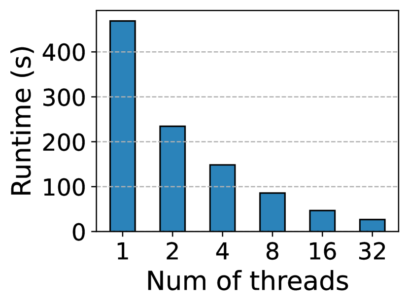
(a) BI

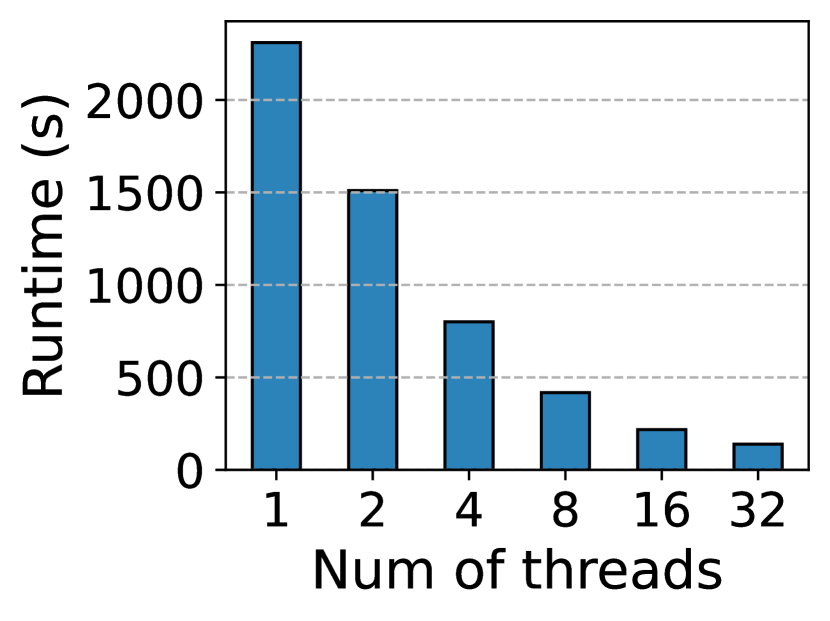
(b) RE

Figure 4: Runtime (in seconds) of the multi-threaded TEACUPS algorithm by varying the number of threads.

Insights from Motif Counts. The count of multi-graph motif instances is significantly higher than that of non-multi-graph motif instances. For example, in the WT dataset with $\delta=4W$, the count for the multi-graph 4-cycle motif, $M_{\text{4-2}}$, is 400 billion, while the count for the simple directed 4-cycle $M_{\text{4-0}}$ is only 300 million. This means the multi-graph 4-cycle motif count is a thousand times larger than the non-multi-graph 4-cycle count, highlighting the dramatic increase in complexity when dealing with multi-graph temporal motifs and underscoring the limitations of previous methods.

When analyzing multi-graph triangle motifs $M_{\text{3-0}}$ and $M_{\text{3-1}}$, changing the order and direction of edges results in different motif counts. For instance, in the WT dataset with $\delta=4W$, the count for $M_{\text{3-1}}$ is approximately 30% higher than that of $M_{\text{3-0}}$. Conversely, in the BI dataset with $\delta=1D$, the count for $M_{\text{3-1}}$ is an order of magnitude lower than that of $M_{\text{3-0}}$. The fast and accurate nature of our algorithm enables getting these interesting insights rapidly to data scientists that can be further used in various downstream tasks (e.g., explaining graph neural networks [60]).

VII Conclusion

This paper presented TEACUPS, a path sampling algorithm to estimate temporal motif counts accurately and efficiently to address the scalability challenge. TEACUPS exhibits a speedup of up to three orders of magnitude over the exact count algorithm with a relative error less than 10%, outperforming both exact and approximate state-of-the-art techniques.

References

- [1] R. Milo, S. Shen-Orr, S. Itzkovitz, N. Kashtan, D. Chklovskii, and U. Alon, “Network motifs: simple building blocks of complex networks,” Science, 2002.
- [2] S. S. Shen-Orr, R. Milo, S. Mangan, and U. Alon, “Network motifs in the transcriptional regulation network of escherichia coli,” Nature genetics, 2002.
- [3] U. Alon, “Network motifs: theory and experimental approaches,” Nature Reviews Genetics, 2007.
- [4] M. E. Newman, “The structure and function of complex networks,” SIAM review, 2003.
- [5] A. P. Iyer, Z. Liu, X. Jin, S. Venkataraman, V. Braverman, and I. Stoica, “ASAP: Fast, approximate graph pattern mining at scale,” in OSDI, 2018.
- [6] M. Jha, C. Seshadhri, and A. Pinar, “Path sampling: A fast and provable method for estimating 4-vertex subgraph counts,” in WWW, 2015.
- [7] A. Pinar, C. Seshadhri, and V. Vishal, “Escape: Efficiently counting all 5-vertex subgraphs,” in WWW, 2017.
- [8] P. Wang, J. Zhao, X. Zhang, Z. Li, J. Cheng, J. C. Lui, D. Towsley, J. Tao, and X. Guan, “Moss-5: A fast method of approximating counts of 5-node graphlets in large graphs,” IEEE Transactions on Knowledge and Data Engineering, 2017.
- [9] S. Jain and C. Seshadhri, “The power of pivoting for exact clique counting,” in ICDM, 2020.
- [10] M. Bressan, F. Chierichetti, R. Kumar, S. Leucci, and A. Panconesi, “Motif counting beyond five nodes,” TKDD, 2018.
- [11] C. Seshadhri and S. Tirthapura, “Scalable subgraph counting: The methods behind the madness: Www 2019 tutorial,” in WWW, 2019.
- [12] L. Kovanen, M. Karsai, K. Kaski, J. Kertész, and J. Saramäki, “Temporal motifs in time-dependent networks,” Journal of Statistical Mechanics: Theory and Experiment, 2011.
- [13] R. K. Pan and J. Saramäki, “Path lengths, correlations, and centrality in temporal networks,” Physical Review E, 2011.
- [14] L. Kovanen, K. Kaski, J. Kertész, and J. Saramäki, “Temporal motifs reveal homophily, gender-specific patterns, and group talk in call sequences,” 2013.
- [15] M. Lahiri and T. Y. Berger-Wolf, “Structure prediction in temporal networks using frequent subgraphs,” in CIDM, 2007.
- [16] A. Paranjape, A. R. Benson, and J. Leskovec, “Motifs in temporal networks,” in WSDM, 2017.
- [17] L. Hajdu and M. Krész, “Temporal network analytics for fraud detection in the banking sector,” in TPDL. Springer, 2020.
- [18] P. Liu, R. Acharyya, R. E. Tillman, S. Kimura, N. Masuda, and A. E. Sarıyüce, “Temporal motifs for financial networks: A study on mercari, jpmc, and venmo platforms,” arXiv, 2023.
- [19] Y. Hulovatyy, H. Chen, and T. Milenković, “Exploring the structure and function of temporal networks with dynamic graphlets,” Bioinformatics, 2015.
- [20] G. Bouritsas, F. Frasca, S. P. Zafeiriou, and M. Bronstein, “Improving graph neural network expressivity via subgraph isomorphism counting,” IEEE Transactions on Pattern Analysis and Machine Intelligence, 2022.
- [21] E. Rossi, B. Chamberlain, F. Frasca, D. Eynard, F. Monti, and M. Bronstein, “Temporal graph networks for deep learning on dynamic graphs,” arXiv, 2020.
- [22] C. Seshadhri, A. Pinar, and T. G. Kolda, “Wedge sampling for computing clustering coefficients and triangle counts on large graphs,” Statistical Analysis and Data Mining: The ASA Data Science Journal, 2014.
- [23] R. Kumar and T. Calders, “2scent: An efficient algorithm to enumerate all simple temporal cycles,” VLDB, 2018.
- [24] N. Pashanasangi and C. Seshadhri, “Faster and generalized temporal triangle counting, via degeneracy ordering,” in KDD, 2021.
- [25] P. Mackey, K. Porterfield, E. Fitzhenry, S. Choudhury, and G. Chin, “A chronological edge-driven approach to temporal subgraph isomorphism,” in Big Data. IEEE, 2018.
- [26] A. Turk and D. Turkoglu, “Revisiting wedge sampling for triangle counting,” in WWW, 2019.
- [27] X. Chen et al., “Efficient and scalable graph pattern mining on GPUs,” in OSDI, 2022.
- [28] K. Jamshidi, R. Mahadasa, and K. Vora, “Peregrine: a pattern-aware graph mining system,” in Proceedings of the Fifteenth European Conference on Computer Systems, 2020.
- [29] K. Jamshidi and K. Vora, “A deeper dive into pattern-aware subgraph exploration with peregrine,” ACM SIGOPS Operating Systems Review, 2021.
- [30] D. Mawhirter, S. Reinehr, C. Holmes, T. Liu, and B. Wu, “Graphzero: Breaking symmetry for efficient graph mining,” arXiv, 2019.
- [31] D. Mawhirter and B. Wu, “Automine: harmonizing high-level abstraction and high performance for graph mining,” in SOSP, 2019.
- [32] T. Shi, M. Zhai, Y. Xu, and J. Zhai, “Graphpi: High performance graph pattern matching through effective redundancy elimination,” in SC20: International Conference for High Performance Computing, Networking, Storage and Analysis. IEEE, 2020.
- [33] C. H. Teixeira, A. J. Fonseca, M. Serafini, G. Siganos, M. J. Zaki, and A. Aboulnaga, “Arabesque: a system for distributed graph mining,” in SOSP, 2015.
- [34] Y. Wei and P. Jiang, “Stmatch: accelerating graph pattern matching on gpu with stack-based loop optimizations,” in SC, 2022.
- [35] Q. Li and J. X. Yu, “Fast local subgraph counting,” VLDB, 2024.
- [36] T. Schank and D. Wagner, “Finding, counting and listing all triangles in large graphs, an experimental study,” in Experimental and Efficient Algorithms. Springer, 2005.
- [37] P. Liu, A. R. Benson, and M. Charikar, “Sampling methods for counting temporal motifs,” in WSDM, 2019.
- [38] J. Wang, Y. Wang, W. Jiang, Y. Li, and K.-L. Tan, “Efficient sampling algorithms for approximate temporal motif counting,” in CIKM, 2020.
- [39] C. E. Tsourakakis, U. Kang, G. L. Miller, and C. Faloutsos, “Doulion: counting triangles in massive graphs with a coin,” in KDD, 2009.
- [40] N. K. Ahmed, N. Duffield, J. Neville, and R. Kompella, “Graph sample and hold: A framework for big-graph analytics,” in KDD, 2014.
- [41] A. Pavan, K. Tangwongsan, S. Tirthapura, and K.-L. Wu, “Counting and sampling triangles from a graph stream,” VLDB, 2013.
- [42] S. Jain and C. Seshadhri, “A fast and provable method for estimating clique counts using turán’s theorem,” in WWW, 2017.
- [43] X. Ye, R.-H. Li, Q. Dai, H. Chen, and G. Wang, “Lightning fast and space efficient k-clique counting,” in WWW, 2022.
- [44] X. Ye, R.-H. Li, Q. Dai, H. Qin, and G. Wang, “Efficient biclique counting in large bipartite graphs,” Proceedings of the ACM on Management of Data, 2023.
- [45] Y. Yang, Y. Fang, M. E. Orlowska, W. Zhang, and X. Lin, “Efficient bi-triangle counting for large bipartite networks,” VLDB, 2021.
- [46] M. Bressan, S. Leucci, and A. Panconesi, “Motivo: fast motif counting via succinct color coding and adaptive sampling,” VLDB, 2019.
- [47] Y. Yuan, H. Ye, S. Vedula, W. Kaza, and N. Talati, “Everest: Gpu-accelerated system for mining temporal motifs,” VLDB, 2023.
- [48] X. Sun, Y. Tan, Q. Wu, B. Chen, and C. Shen, “Tm-miner: Tfs-based algorithm for mining temporal motifs in large temporal network,” IEEE Access, 2019.
- [49] S. Min, J. Jang, K. Park, D. Giammarresi, G. F. Italiano, and W.-S. Han, “Time-constrained continuous subgraph matching using temporal information for filtering and backtracking,” arXiv, 2023.
- [50] H. D. Boekhout, W. A. Kosters, and F. W. Takes, “Efficiently counting complex multilayer temporal motifs in large-scale networks,” Computational Social Networks, 2019.
- [51] Z. Gao, C. Cheng, Y. Yu, L. Cao, C. Huang, and J. Dong, “Scalable motif counting for large-scale temporal graphs,” in ICDE. IEEE, 2022.
- [52] I. Sarpe and F. Vandin, “Presto: Simple and scalable sampling techniques for the rigorous approximation of temporal motif counts,” in SDM, 2021.
- [53] N. K. Ahmed, N. Duffield, and R. A. Rossi, “Online sampling of temporal networks,” TKDD, 2021.
- [54] D. Dubhashi and A. Panconesi, Concentration of measure for the analysis of randomized algorithms, 2009.
- [55] J. Leskovec and A. Krevl, “SNAP Datasets: Stanford large network dataset collection,” http://snap.stanford.edu/data, Jun. 2014.
- [56] D. Kondor, I. Csabai, J. Szüle, M. Pósfai, and G. Vattay, “Inferring the interplay between network structure and market effects in bitcoin,” New Journal of Physics, 2014.
- [57] J. Hessel, C. Tan, and L. Lee, “Science, askscience, and badscience: On the coexistence of highly related communities,” in ICWSM, 2016.
- [58] “PRESTO Code,” https://github.com/VandinLab/PRESTO, 2021.
- [59] “Everest Code,” https://github.com/yichao-yuan-99/Everest, 2023.
- [60] J. Chen and R. Ying, “Tempme: Towards the explainability of temporal graph neural networks via motif discovery,” Advances in Neural Information Processing Systems, 2024.