A Near-Optimal Algorithm for Convex Simple Bilevel Optimization under Weak Assumptions

Abstract

Bilevel optimization provides a comprehensive framework that bridges single- and multi-objective optimization, encompassing various formulations, including standard nonlinear programs. This paper focuses on a specific class of bilevel optimization known as simple bilevel optimization. In these problems, the objective is to minimize a composite convex function over the optimal solution set of another composite convex minimization problem. By reformulating the simple bilevel problem as finding the left-most root of a nonlinear equation, we employ a bisection scheme to efficiently obtain a solution that is $\epsilon$-optimal for both the upper- and lower-level objectives. In each iteration, the bisection narrows down an interval by assessing the feasibility of a discriminating criterion. By introducing a novel dual approach and employing the Accelerated Proximal Gradient (APG) method, we demonstrate that each subproblem in the bisection scheme can be solved in ${\mathcal{O}}(\sqrt{(L_{g_{1}}+2D_{z}L_{f_{1}}+1)/\epsilon}|\log\epsilon|^{2})$ oracle queries under weak assumptions. Here, $L_{f_{1}}$ and $L_{g_{1}}$ represent the Lipschitz constants of the gradients of the upper- and lower-level objectives’ smooth components, and $D_{z}$ is the upper bound of the optimal multiplier of the subproblem. Considering the number of binary searches, the total complexity of our proposed method is ${\mathcal{O}}(\sqrt{(L_{g_{1}}+2D_{z}L_{f_{1}}+1)/\epsilon}|\log\epsilon|^{3})$. Our method achieves near-optimal complexity results, comparable to those in unconstrained smooth or composite convex optimization when disregarding the logarithmic terms. Numerical experiments also demonstrate the superior performance of our method compared to the state-of-the-art.

1 Introduction

Bilevel optimization problems are hierarchically structured, consisting of two nested optimization tasks: the upper- and lower-level problems. The upper-level problem aims to find an optimal solution within the feasible region defined by the solutions set of the lower-level problem. Originating in game theory, these problems have been extensively studied since the 1950s, as documented by foundational works such as [14, 15]. Recent applications have expanded into diverse areas of machine learning, including hyperparameter optimization [22, 49, 21], meta-learning [22, 5, 45], data poisoning attacks [38, 40], reinforcement learning [31, 26], and adversarial learning [8, 56, 57]. Additionally, the study of variational inequality formulations of bilevel problems has garnered significant interest [20, 7, 32, 28, 43]. For a recent and comprehensive review of bilevel optimization and its applications, one may refer to [15] and the references therein. Further discussions on various applications pertinent to this paper can be found in recent literature [1, 63, 51].

In this paper, we focus on a specific class of bilevel optimization problems where the lower-level problem does not depend parametrically on the variables of the upper-level problem. This class, often referred to as “simple bilevel optimization” in the literature [17, 19, 50, 27, 58, 13], is a subset of general bilevel optimization problems. It has also garnered significant interest in the machine learning community, with applications in dictionary learning [3, 27], lexicographic optimization [29, 24], lifelong learning [37, 27], and the applications mentioned above. Specifically, we are interested in the following convex composite minimization problem:

$$\begin{array}[]{lcl}&\min\limits_{\mathbf{x}\in\mathbb{R}^{n}}&f(\mathbf{x})\triangleq f_{1}(\mathbf{x})+f_{2}(\mathbf{x})\\ &{\rm s.t.}&\mathbf{x}\in\operatorname*{arg\,min}\limits_{\mathbf{z}\in\mathbb{R}^{n}}g(\mathbf{z})\triangleq g_{1}(\mathbf{z})+g_{2}(\mathbf{z}).\end{array}$$ (1)

Here, functions $f_{1}$ and $g_{1}:X\rightarrow\mathbb{R}$ are convex and continuously differentiable over an open set $X\subseteq\mathbb{R}^{n}$. Their gradients, $\nabla f_{1}$ and $\nabla g_{1}$, are $L_{f_{1}}$- and $L_{g_{1}}$-Lipschitz continuous, respectively. Functions $f_{2}$ and $g_{2}:\mathbb{R}^{n}\rightarrow\mathbb{R}\cup\{\infty\}$ are proper lower semicontinuous (l.s.c.) convex functions with tractable proximal operators. We assume that $g$ is not strongly convex and that the lower-level problem has multiple optimal solutions [27, 58, 13]. In other words, the optimal solution set of the lower-level problem, denoted as $X_{g}^{*}$, is not a singleton. Otherwise, the optimal minimum is determined by the lower-level problem.

Particularly, let $p^{*}$ be the optimal value of Problem (1) and $g^{*}$ be the optimal value of the unconstrained lower-level problem

$$\min_{\mathbf{x}\in\mathbb{R}^{n}}~{}g(\mathbf{x})\triangleq g_{1}(\mathbf{x})+g_{2}(\mathbf{x}).$$ (2)

The goal of this paper is to find an $(\epsilon_{f},\epsilon_{g})$-optimal solution $\widehat{\mathbf{x}}$ of Problem (1) defined as follows.

Definition 1 ($(\epsilon_{f},\epsilon_{g})$-optimal solution).

A point $\widehat{\mathbf{x}}$ is called an $(\epsilon_{f},\epsilon_{g})$-optimal solution of Problem (1), if it satisfies

$$f(\widehat{\mathbf{x}})-p^{*}\leq\epsilon_{f}~{}~{}\text{and}~{}~{}g(\widehat{\mathbf{x}})-g^{*}\leq\epsilon_{g}.$$

A potential approach to solving Problem (1) involves reformulating it as a single-level constrained convex optimization problem, followed by the application of primal-dual methods. Specifically, Problem (1) can be transformed into a constrained convex optimization problem as follows:

$$\min_{\mathbf{x}\in\mathbb{R}^{n}}f(\mathbf{x})~{}~{}{\rm s.t.}~{}~{}g(\mathbf{x})\leq g^{*}.$$ (3)

When directly implementing primal-dual-type methods, a critical concern is the noncompliance of Problem (3) with the necessary regularity conditions for convergence. This issue arises from the absence of strict feasibility, leading to the failure of Slater’s condition. Moreover, traditional first-order algorithms, such as projected gradient descent, often prove impractical due to the computational complexity involved in orthogonally projecting onto the level set of the subordinated objective. To mitigate this issue, one might consider relaxing the constraint to ensure strict feasibility,

$$\min_{\mathbf{x}\in\mathbb{R}^{n}}f(\mathbf{x})~{}~{}{\rm s.t.}~{}~{}g(\mathbf{x})\leq g^{*}+\varepsilon,$$ (4)

the challenge remains. Indeed, as $\varepsilon$ approaches zero, rendering the problem nearly degenerate, the dual optimal variable may tend toward infinity. This phenomenon impedes convergence and leads to numerical instability [9]. Consequently, Problem (1) cannot be directly addressed as a conventional constrained optimization problem; it necessitates the development of new theories and algorithms tailored to its hierarchical structure.

1.1 Our Approach

We first exchange the roles of the upper- and lower-level objectives in Problem (1) and consider the following single-level convex optimization problem:

$$\min_{\mathbf{x}\in\mathbb{R}^{n}}~{}g(\mathbf{x}),~{}~{}{\rm s.t.}~{}~{}f(\mathbf{x})\leq c.$$ (5)

We then recast Problem (1) in terms of the value function for Problem (5):

$$\bar{g}(c):=\min_{\mathbf{x}\in\mathbb{R}^{n}}~{}\{g(\mathbf{x})~{}|~{}f(\mathbf{x})\leq c\}.$$ (6)

The univariate value function $\bar{g}(c)$ is non-increasing and convex [46]. Furthermore, the optimal value of Problem (1) is the left-most root of the following nonlinear equation:

$$\bar{g}(c)=g^{*}.$$ (7)

This observation leads to a general framework for solving Problem (1), where any root-finding algorithm may be applied. Given that the lower-level problem has multiple optimal solutions, multiple roots must exist for (7). However, only the left-most root is valid. Several root-finding algorithms can locate the left-most root of Problem (7), such as the bisection method, Newton’s method, secant method, and their variants [30]. In this paper, we select the bisection method as the root-finding algorithm, while the Newton and secant methods will be explored in future work. To determine the left-most root of Problem (7), our bisection approach checks the feasibility of the following system:

$$f(\mathbf{x})\leq c,~{}g(\mathbf{x})\leq g^{*}.$$ (8)

We assume that the exact values of both $\bar{g}(c)$ and the optimal value $g^{*}$ from the unconstrained lower-level problem (2) are given. If $\bar{g}(c)>g^{*}$, System (8) is infeasible, and $c$ acts as a lower bound for $p^{*}$. Conversely, if $\bar{g}(c)=g^{*}$, System (8) is feasible, and $c$ acts as an upper bound for $p^{*}$.

The feasibility of System (8) can be assessed by solving Problem (5). The following text provides a comprehensive description of our algorithm, which accounts for the inherent imprecision in solving Problem (5). Furthermore, by applying Accelerated Proximal Gradient (APG) methods [42, 4, 34] to the solvability of Problem (5) and establishing initial lower and upper bounds for $c$, we derive a near-optimal complexity analysis for our algorithm.

Moreover, [58] has developed a bisection-based method for solving Problem (1) under specific assumptions, termed ‘Bisec-BiO’. Specifically, for any fixed $c$, Problem (5) is reformulated into the following form:

$$\min_{\mathbf{x}\in\mathbb{R}^{n}}~{}g_{c}(\mathbf{x})\triangleq g_{1}(\mathbf{x})+g_{2}(\mathbf{x})+{\rm I}_{{\rm Lev}_{f}(c)}(\mathbf{x}),$$ (9)

where ${\rm I}_{{\rm Lev}_{f}(c)}(\mathbf{x})$ is the indicator function of ${\rm Lev}_{f}(c)$. In [58, Assumption 1(iv)], they assume that the function $h_{c}(\mathbf{x})=g_{2}(\mathbf{x})+{\rm I}_{{\rm Lev}_{f}(c)}(\mathbf{x})$ is proximal-friendly, and subsequently employ the Accelerated Proximal Gradient (APG) method [42, 4, 34] to solve Problem (9) as a subroutine in the bisection scheme. However, the assumption that the function $h_{c}(\mathbf{x})=g_{2}(\mathbf{x})+{\rm I}_{{\rm Lev}_{f}(c)}(\mathbf{x})$ is proximal-friendly can be challenging (for example, when the upper-level objective is the least square loss function). In this paper, we propose an alternative reformulation of Problem (5) to address Problem (1) under more general settings while maintaining comparable complexity results.

1.1.1 Overview of The Proposed Method

As previously discussed, [58, Assumption 1(iv)] may be challenging to fulfill in the context of a complex upper-level objective. To address this issue, we employ a dual approach to solve the following perturbed strongly convex problem of (5) with a given error tolerance $\epsilon>0$:

$$\begin{array}[]{lcl}&\min\limits_{\mathbf{x}\in\mathbb{R}^{n}}&G_{\epsilon}(\mathbf{x})\triangleq g_{\epsilon}(\mathbf{x})+g_{2}(\mathbf{x})\\ &{\rm s.t.}&f_{c}(\mathbf{x})=f_{1}(\mathbf{x})-c+f_{2}(\mathbf{x})\leq 0,\end{array}$$ (10)

where $g_{\epsilon}(\mathbf{x})=g_{1}(\mathbf{x})+\frac{\epsilon}{2}\|\mathbf{x}-\mathbf{x}^{0}\|^{2}$ and $\mathbf{x}^{0}$ is a point that belongs to a level set of the unconstrained lower-level problem (2).

The Lagrange-dual reformulation of Problem (10) is

$$\min_{\mathbf{x}\in\mathbb{R}^{n}}\max_{z\geq 0}\mathcal{L}^{\epsilon}(\mathbf{x},z)\triangleq G_{\epsilon}(\mathbf{x})+zf_{c}(\mathbf{x})=g_{\epsilon}(\mathbf{x})+z(f_{1}(\mathbf{x})-c)+g_{2}(\mathbf{x})+zf_{2}(\mathbf{x}),$$ (11)

where $z\geq 0$ is the multiplier. In this scenario, it suffices to assume that the proximal mapping of $g_{2}(\mathbf{x})+zf_{2}(\mathbf{x})$ is proximal-friendly [10, 33, 13], which is a less restrictive requirement than [58, Assumption 1(iv)].

To solve Problem (11), we first identify an interval that encompasses the optimal multiplier of Problem (10) (cf. Algorithm 3). Within this interval, we then perform a binary search to obtain an approximate solution that satisfies the approximate Karush-Kuhn-Tucker (KKT) conditions of Problem (10) (cf. Algorithm 4). This approximate solution is also shown to be equivalent to an approximate solution of Problem (5). For further details, please refer to Sections 3 and 4.

1.2 Related Work

One category of algorithms for solving Problem (1) is based on solving the Tikhonov-type regularization [54]:

$$\min_{\mathbf{x}\in\mathbb{R}^{n}}\phi_{k}(\mathbf{x})\triangleq g(\mathbf{x})+\lambda_{k}f(\mathbf{x}),$$ (12)

for each regularization parameter $\lambda_{k}>0$. Here, $\lambda_{k}$ satisfies the “slow condition” that $\lim_{k\rightarrow\infty}\lambda_{k}=0$ and $\sum_{k=1}^{\infty}\lambda_{k}=\infty$. [52] introduced the Iterative Regularized Projected Gradient (IR-PG) method, which applies a projected gradient step to the Tikhonov-type regularization problem (12) at each iteration. This method assumes that the upper-level objective is $L$-smooth and the non-smooth term of the lower-level objective is the indicator function of a closed convex set. Under the same non-smooth term of the lower-level objective and the additional assumption that both the upper- and lower-level objectives have bounded (sub)gradients, [25] proposed a three-step variation of the $\epsilon$-subgradient method, which involves accelerated-gradient, (sub)gradient or proximal gradient, and projection steps. Additionally, [24] presented the dynamic barrier gradient descent (DBGD) method for continuously differentiable upper- and lower-level objectives, which also converges to the optimal set of Problem (1). However, these algorithms do not offer non-asymptotic guarantees for either the upper or lower-level objective. For a comprehensive overview of these methods, please refer to [18, 27] and the references therein.

Another class of algorithms establishes a non-asymptotic convergence rate for the lower-level objective and an asymptotic convergence rate for the upper-level objective of Problem (1). [3] introduced the minimal norm gradient (MNG) method for cases where the upper-level objective is differentiable and strongly convex, and the lower-level objective is smooth. They proved that MNG asymptotically converges to the optimal solution of Problem (1) and achieves a convergence rate of ${\mathcal{O}}({L_{g_{1}}^{2}}/{\epsilon^{2}})$ to reach an $\epsilon$-optimal solution for the lower-level problem. Building on the sequential averaging method (SAM) framework, [47] developed the bilevel gradient sequential averaging method (BiG-SAM) for cases with a strongly convex upper-level objective and a composite lower-level objective. They achieved a convergence rate of ${\mathcal{O}}(L_{g_{1}}/\epsilon)$ to reach an $\epsilon$-optimal solution for the lower-level problem. They also demonstrated that by replacing the upper-level objective with its Moreau envelope [2, Definition 6.52] when the upper-level objective is non-smooth, the convergence rate of BiG-SAM to reach an $\epsilon$-optimal solution for the lower-level objective is ${\mathcal{O}}(L_{g_{1}}/\epsilon\delta^{2})$, where $\delta>0$ is the parameter in the Moreau envelope of the upper-level objective. [1] extended the IR-PG [52] method for cases with a strongly convex but not necessarily differentiable upper-level objective and a finite-sum lower-level objective. They proposed the iterative regularized incremental projected (sub)gradient (IR-IG) method, which achieves a convergence rate of ${\mathcal{O}}(1/\epsilon^{\frac{1}{0.5-b}})$ to reach an $\epsilon$-optimal solution for the lower-level objective, where $b\in(0,0.5)$. Assuming that both objectives are composite, [37] studied a version of Tseng’s accelerated gradient method that achieves a convergence rate of ${\mathcal{O}}(1/\epsilon)$ to produce an $\epsilon$-optimal solution for the lower-level problem. Therefore, previous studies have mainly focused on the convergence rates of the lower-level problem while largely neglecting those for the upper-level objective.

Recently, several algorithms have been developed to analyze non-asymptotic convergence rates for both upper- and lower-level objectives. Within the Lipschitz continuity of the objectives, [28] demonstrated that their averaging iteratively regularized gradient (a-IRG) method can achieve a convergence rate of $\mathcal{O}(\max\{1/\epsilon_{f}^{\frac{1}{0.5-b}},1/\epsilon_{g}^{\frac{1}{b}}\})$ to obtain an $(\epsilon_{f},\epsilon_{g})$-optimal solution of Problem (1), where $b\in(0,0.5)$. By assuming a global error-bound condition and a “norm-like” property for the upper-level objective (e.g., the elastic-net $\|\mathbf{x}\|_{1}+\rho\|\mathbf{x}\|^{2}$), [18] introduced the iterative approximation and level set expansion (ITALEX) scheme to tackle Problem $\eqref{p:primal}$ with composite objectives. Their algorithm demonstrates a convergence rate of $\mathcal{O}(1/\epsilon^{2})$ to produce an $(\epsilon,\epsilon)$-optimal solution of Problem (1). Inspired by [28], [39] proposed a bi-sub-gradient (Bi-SG) method under a quasi-Lipschitz assumption for the upper-level objective, achieving a convergence rate of $\mathcal{O}(\max\{1/\epsilon_{f}^{\frac{1}{1-a}},1/\epsilon_{g}^{\frac{1}{a}}\})$ to achieve an $(\epsilon_{f},\epsilon_{g})$-optimal solution of Problem (1), where $a\in(0.5,1)$. Furthermore, when the upper-level objective is assumed to be $\mu$-strongly convex, the convergence rate of the upper-level objective can be improved to be linear. [27] introduced a conditional gradient-based bilevel optimization (CG-BiO) method, which necessitates $\mathcal{O}(\max\{L_{f_{1}}/\epsilon_{f},L_{g_{1}}/\epsilon_{g}\})$ iterations to achieve an $(\epsilon_{f},\epsilon_{g})$-optimal solution of Problem (1). In their problem setting, both the upper- and lower-level objectives are smooth, and the domain of the lower-level objective is compact. Within similar problem settings of [27], [23] proposed an iteratively regularized conditional gradient (IR-CG) method, ensuring a convergence rate of $\mathcal{O}(\max\{1/\epsilon_{f}^{\frac{1}{1-p}},1/\epsilon_{g}^{\frac{1}{p}}\})$ to produce an $(\epsilon_{f},\epsilon_{g})$-optimal solution of Problem (1), where $p\in(0,1)$. [51] combined an online framework with the mirror descent algorithm, establishing a convergence rate of $\mathcal{O}(\max\{1/\epsilon_{f}^{3},\epsilon_{g}^{3}\})$ to produce an $(\epsilon_{f},\epsilon_{g})$-optimal solution of Problem (1), assuming a compact domain and boundedness of the functions and gradients at both upper- and lower-level objectives. Additionally, they demonstrated that the convergence rate can be enhanced to $\mathcal{O}(\max\{1/\epsilon_{f}^{2},1/\epsilon_{g}^{2}\})$ under additional structural assumptions.

Very recently, several papers have proposed significantly improved complexity results. By assuming weak-sharp minima [53] for the lower-level problem, [48] introduced a regularized accelerated proximal method (R-APM) to address the Tikhonov-type regularization problem (12). They demonstrated convergence rates of $\mathcal{O}(\epsilon^{-0.5})$ for both upper and lower-level objectives in achieving an $\epsilon$-optimal solution of Problem (1). Assuming the $\alpha$-Hölderian error bound condition of the lower-level objective with $\alpha\geq 1$, [13] proposed a penalty-based accelerated proximal gradient (PB-APG) method. This method exhibited convergence rates of $\mathcal{O}(\sqrt{{L_{f_{1}}}/{\epsilon}}+\sqrt{{l_{f}^{\max\{\alpha,\beta\}}L_{g_{1}}}/{\epsilon^{\max\{\alpha,\beta\}}}})$ for both upper and lower-level objectives to find an $(\epsilon,\epsilon^{\beta})$-optimal solution of Problem (1) for any given $\beta>0$. Here, $l_{f}$ represents the upper bound of the (sub)gradients of the upper-level objective. If the upper-level objective is assumed to be $\mu$-strongly convex, the complexity can be enhanced to $\tilde{\mathcal{O}}(\sqrt{{L_{f_{1}}}/{\mu}}+\sqrt{{l_{f}^{\max\{\alpha,\beta\}}L_{g_{1}}}/{\epsilon^{\max\{\alpha-1,\beta-1\}}}})$, where $\tilde{\mathcal{O}}$ omits a logarithmic term. Furthermore, in cases where both the lower- and upper-level objectives are non-smooth, the convergence rate is $\mathcal{O}({{l_{f_{2}}^{2}}/{\epsilon^{2}}}+{{l_{f_{2}}^{\max\{2\alpha,2\beta\}}l_{g_{2}}^{2}}/{\epsilon^{\max\{2\alpha,2\beta\}}}})$, where $l_{f_{2}}$ and $l_{g_{2}}$ are the Lipschitz constants of the upper- and lower-level objectives, respectively. Following the same assumptions adopted in [27], the accelerated gradient method for bilevel optimization (AGM-BiO) proposed by [11] achieved convergence rates of $\mathcal{O}(\max\{1/\sqrt{\epsilon_{f}},1/\epsilon_{g}\})$ to achieve an $(\epsilon_{f},\epsilon_{g})$-optimal solution of Problem (1). By incorporating an additional $\alpha$-Hölderian error bound condition of the lower-level objective, their complexity can be improved to $\mathcal{O}(\max\{1/\epsilon_{f}^{-\frac{2\alpha-1}{2\alpha}},1/\epsilon_{g}^{-\frac{2\alpha-1}{2\alpha}}\})$.

For a comprehensive overview of the methods above (including only non-asymptotic convergence rates for both upper- and lower-level objectives), detailing their underlying assumptions and resulting convergence outcomes, please refer to Table 1.

Table 1: Summary of simple bilevel optimization algorithms. The abbreviations “SC”, “C”, “diff”, “comp”, “Lip”, “WS”, “C3”, and “$\alpha$-HEB” represent “strongly convex”, “convex”, “differentiable”, “composite”, “Lipschitz”, “weak sharpness”, “Convex objective with Convex Compact constraints”, and “Hölderian error bound with exponent parameter $\alpha$”, respectively. Notations $l_{f}$, $L_{f_{1}}$, and $L_{g_{1}}$ are the Lipschitz constants of $f$, $\nabla f_{1}$, and $\nabla g_{1}$, respectively. We include the Lipschitz constant only when its relevance to complexity is evident; otherwise, we omit it.

Methods	Upper-level	Lower-level	$(\epsilon_{f},\epsilon_{g})$-optimal	Convergence Rates
	Objective $f$	Objective $g$	Solution	Upper-level	Lower-level
IR-CG [23]	C, smooth	C3, smooth	$(\epsilon_{f},\epsilon_{g})$	$\mathcal{O}\left(\max\{{1}/{\epsilon_{f}^{\frac{1}{1-p}}},{1}/{\epsilon_{g}^{\frac{1}{p}}}\}\right)$, $p\in(0,1)$
ITALEX [18]	C, comp	C, comp	$(\epsilon,\epsilon^{2})$	$\mathcal{O}\left(1/\epsilon^{2}\right)$
a-IRG [28]	C, Lip	C, Lip	$(\epsilon_{f},\epsilon_{g})$	${\mathcal{O}}\left(\max\{1/\epsilon_{f}^{\frac{1}{0.5-b}},1/\epsilon_{g}^{\frac{1}{b}}\}\right)$, $b\in(0,0.5)$
CG-BiO [27]	C, smooth	C3, smooth	$(\epsilon_{f},\epsilon_{g})$	${\mathcal{O}}\left(\max\{L_{f_{1}}/\epsilon_{f},L_{g_{1}}/\epsilon_{g}\}\right)$
Bi-SG [39]	C, quasi-Lip/comp	C, comp	$(\epsilon_{f},\epsilon_{g})$	$\mathcal{O}\left(\max\{1/\epsilon_{f}^{\frac{1}{1-a}},1/\epsilon_{g}^{\frac{1}{a}}\}\right)$, $a\in(0.5,1)$
	$\mu$-SC, comp	C, comp	$(\epsilon_{f},\epsilon_{g})$	$\mathcal{O}\left(\max\{\left(\frac{\log 1/\epsilon_{f}}{\mu}\right)^{\frac{1}{1-a}},1/\epsilon_{g}^{\frac{1}{a}}\}\right),a\in(0.5,1)$
Online Framework [51]	C, Lip	C3, Lip	$(\epsilon_{f},\epsilon_{g})$	$\mathcal{O}\left(\max\{1/\epsilon_{f}^{3},1/\epsilon_{g}^{3}\}\right)$
R-APM [48]	C, smooth	C, comp, WS	$(\epsilon,\epsilon)$	$\mathcal{O}\left(\max\{L_{f_{1}}/\epsilon^{0.5},L_{g_{1}}/\epsilon^{0.5}\}\right)$
PB-APG [13]	C, comp, Lip	C, comp, $\alpha$-HEB	$(\epsilon,l_{f}^{-\beta}\epsilon^{\beta})$	$\mathcal{O}\left(\max\{\sqrt{\frac{L_{f_{1}}}{\epsilon}},\sqrt{\frac{l_{f}^{\max\{\alpha,\beta\}}L_{g_{1}}}{\epsilon^{\max\{\alpha,\beta\}}}}\}\right)$
	$\mu$-SC, comp, Lip	C, comp, $\alpha$-HEB	$(\epsilon,l_{F}^{-\beta}\epsilon^{\beta})$	${\mathcal{O}}\left(\sqrt{\frac{L_{f_{1}}}{\mu}}\log\frac{1}{\epsilon}\right)+{\mathcal{O}}\left(\sqrt{\frac{l_{F}^{\max\{\alpha,\beta\}}L_{g_{1}}}{\epsilon^{\max\{\alpha-1,\beta-1\}}}}\log\frac{1}{\epsilon}\right)$
AGM-BiO [11]	C, smooth	C3, smooth	$(\epsilon_{f},\epsilon_{g})$	$\tilde{\mathcal{O}}\left(\max\{1/\sqrt{\epsilon_{f}},1/\epsilon_{g}\}\right)$
	C, smooth	C, smooth, $\alpha$-HEB	$(\epsilon_{f},\epsilon_{g})$	$\tilde{\mathcal{O}}\left(\max\{1/\epsilon_{f}^{-\frac{2\alpha-1}{2\alpha}},1/\epsilon_{g}^{-\frac{2\alpha-1}{2\alpha}}\}\right)$
Bisec-BiO [58]	C, comp	C, comp	$(\epsilon_{f},\epsilon_{g})$	${\mathcal{O}}\left(\max\{\sqrt{L_{f_{1}}/\epsilon_{f}},\sqrt{L_{g_{1}}/\epsilon_{g}}\}|\log\epsilon_{f}|\right)$
BiVFA (Ours)	C, comp	C, comp	$(\epsilon,\epsilon)$	${\mathcal{O}}\left(\sqrt{{{(L_{g_{1}}+2D_{z}L_{f_{1}}+1)}}/{{\epsilon}}}|\log\epsilon|^{3}\right)$

1.3 Contributions and Outline

This paper proposes a Biection method based Value Function Algorithm (BiVFA) for solving Problem (1). The method employs a bisection scheme to find the left-most root of a nonlinear equation iteratively and incorporates a novel dual approach to address Problem (5) as a subroutine. Our proposed method demonstrates superior convergence rates compared to existing literature, as detailed in Table 1. The specific contributions are outlined below.

• We introduce a bisection scheme that efficiently determines an $(\epsilon,\epsilon)$-optimal solution for Problem (1), achieving a convergence rate of ${\mathcal{O}}(\sqrt{{(L_{g_{1}}+2D_{z}L_{f_{1}}+1)}/{\epsilon}}|\log\epsilon|^{3})$. Our method provides a near-optimal complexity guarantee for both upper- and lower-level problems. Specifically, our rate aligns with the optimal rate observed in unconstrained smooth or composite convex optimization when omitting the logarithmic terms [41, 59].

• Our proposed method employs weak assumptions. Specifically, it does not require strong convexity or smoothness of the upper-level objective, nor does it necessitate a bounded domain or smoothness of the lower-level objective, as commonly assumed in existing literature.

• We perturb the subproblem in our algorithm as a functionally constrained strongly convex problem and introduce a dual approach to solve it efficiently. We present the best-known complexity results for the functionally constrained strongly convex subproblem without assuming a bounded domain for the lower-level objective, as in [61, Assumption 2].

• The experimental results on various practical application problems demonstrate the superior performance of our proposed method compared to the state-of-the-art techniques.

The remaining sections of the paper are organized as follows. Section 2 revisits the Accelerated Proximal Gradient algorithms for both strongly convex and convex problems, along with their respective convergence rates. Section 3 introduces the bisection scheme proposed for solving Problem (1) and outlines the basic assumptions made in this paper. Section 4 presents a detailed dual approach for solving the subproblem, including the necessary preparatory results for algorithm design. The primary algorithm and its corresponding complexity analysis for addressing Problem (1) are presented in Section 5. Section 6 contains the results of numerical experiments and comparisons with existing methods.

Notations

In this paper, we adopt the following standard notation: Vectors and matrices are represented in bold. The indicator function of a closed and convex set $C$ is denoted by ${\rm I}_{C}$ with the definition that ${\rm I}_{C}=0$ if $\mathbf{x}\in C$ and ${\rm I}_{C}=+\infty$ otherwise. The orthogonal projection of $x$ onto $C$ is denoted by ${\rm P}_{C}(\mathbf{x})=\operatorname*{arg\,min}\{\|\mathbf{y}-\mathbf{x}\|^{2}:\mathbf{y}\in C\}$, and the distance between $x$ and $C$ is denoted by ${\rm dist}(\mathbf{x},C)$. Furthermore, if $C$ is compact, we define its diameter as $D_{C}=\max\{\|\mathbf{x}-\mathbf{y}\|:\forall\mathbf{x},\mathbf{y}\in C\}$. For a given function $f$ and a constant $c$, we denote its level set by ${\rm Lev}_{f}(c)=\{\mathbf{x}:f(\mathbf{x})\leq c\}$ and its domain by ${\rm dom}(f)$. The subdifferential set of $f$ at the point $x$ is denoted as $\partial f(\mathbf{x})$. For a vector $\mathbf{x}\in\mathbb{R}^{n}$ and a matrix $\mathbf{A}\in\mathbb{R}^{m\times n}$, let $\|\mathbf{x}\|$ and $\|\mathbf{A}\|$ represent the $\ell_{2}$-norm of them. Regarding matrix $\mathbf{A}$, its minimum and maximum eigenvalues are denoted as $\lambda_{\min}(\mathbf{A})$ and $\lambda_{\max}(\mathbf{A})$, respectively. For a real number $a$, we denote $[a]_{+}=\max\{a,0\}$, and $\lceil a\rceil_{+}$ is the smallest nonnegative integer greater than or equal to $a$. Moreover, we use $\mathcal{O}$ and $\tilde{\mathcal{O}}$ with their standard meanings, where in the context of complexity results, $\tilde{\mathcal{O}}$ has a similar meaning to $\mathcal{O}$ but suppresses logarithmic terms.

2 Preliminaries

In this paper, we utilize the Accelerated Proximal Gradient (APG) algorithm [55, 4, 35, 12, 34, 61] to approximately solve composite subproblems of the following form:

$$\min_{\mathbf{x}\in\mathbb{R}^{n}}~{}\varphi(\mathbf{x})\triangleq\varphi_{1}(\mathbf{x})+\varphi_{2}(\mathbf{x}),$$ (13)

where the function $\varphi_{1}:X\rightarrow\mathbb{R}$ is $\mu_{\varphi_{1}}$-strongly convex and continuously differentiable on an open set $X\subset\mathbb{R}^{n}$. The gradient $\nabla\varphi_{1}$ is $L_{\varphi_{1}}$-Lipschitz continuous. The function $\varphi_{2}:\mathbb{R}^{n}\rightarrow\mathbb{R}\cup\{\infty\}$ is proper, lower semicontinuous, convex, possibly non-smooth, and proximal-friendly. Here, a function $\psi$ is considered proximal-friendly for a given $t>0$ if the proximal mapping of $t\cdot\psi$, defined as

$${\rm prox}_{t\psi}(\mathbf{y})\triangleq\operatorname*{arg\,min}_{\mathbf{x}\in\mathbb{R}^{n}}\psi(\mathbf{x})+\frac{1}{2t}\|\mathbf{x}-\mathbf{y}\|^{2},$$ (14)

is easy to compute.

In this paper, for solving Problem (13), we employ the accelerated proximal gradient (APG) framework outlined in [61] as described in Algorithm 1, when the strongly convex parameter $\mu_{\varphi_{1}}>0$. For convenience, we denote this algorithm as $\widehat{\mathbf{x}}={\rm APG}_{\mu}(\varphi_{1},\varphi_{2},{L}_{\min},{\mu}_{\varphi_{1}},\gamma_{1},\gamma_{2},\mathbf{y}_{0},\epsilon)$. When $\mu_{\varphi_{1}}=0$ (i.e., $\varphi_{1}$ is convex but not strongly convex), we adopt the fast iterative shrinkage-thresholding algorithm (FISTA) with backtracking [4], as presented in Algorithm 2, and denote it as $\widehat{\mathbf{x}}={\rm APG}_{0}(\varphi_{1},\varphi_{2},{L}_{0},\eta,\mathbf{x}_{0},\epsilon)$.

The convergence result of Algorithm 1 has been established in [61, Corollary 2.3]. In this paper, without assuming a bounded domain of $\varphi_{2}$ in Problem (13), we introduce several technological modifications and provide a similar convergence result for Algorithm 1, as detailed in Section 4.1.1. Additionally, the convergence result of Algorithm 2 has been provided in [4, Theorem 4.4]. For the sake of compactness, we recapitulate this theorem as follows.

Lemma 2.1.

[4, Theorem 4.4] Denote $X_{\varphi}^{*}$ as the optimal solution set of Problem (13) and $\mathbf{x}_{\varphi}^{*}\in X_{\varphi}^{*}$ be any optimal solution. Let $\mathbf{x}_{0}^{\varphi}\in\mathbb{R}^{n}$ be an initial point, suppose that there exists a constant $R\geq 0$ such that $\|\mathbf{x}_{0}^{\varphi}-\mathbf{x}_{\varphi}^{*}\|\leq R$. Let $\{\mathbf{x}_{k}\}$ be the sequence generated by Algorithm 2. Then for any $k\geq 1$, we have

$$\varphi(\mathbf{x}_{k})-\varphi(\mathbf{x}_{\varphi}^{*})\leq\frac{2\eta L_{{\varphi}_{1}}}{(k+1)^{2}}R^{2}.$$

3 Bisection Scheme for Solving Simple Bilevel Problems

According to [58, Algorithm 1], the algorithm proposed in this paper also employs a bisection scheme. However, our paper distinguishes [58] through a unique reformulation of the subproblem (5) and different underlying assumptions. Specifically, as demonstrated in [58, Assumption 1(iv)], the proximal mapping of $g_{2}+{\rm I}_{{\rm Lev}_{f}(c)}$ is assumed to be proximal-friendly. This assumption becomes challenging to fulfill when dealing with complex upper-level objectives, such as linear regression loss or logistic loss functions. Our algorithm relaxes this assumption and proposes a novel dual approach that achieves comparable complexity results.

Problem (5) is equivalent to the following problem,

$$\begin{array}[]{lcl}&\min\limits_{\mathbf{x}\in\mathbb{R}^{n}}&g(\mathbf{x})=g_{1}(\mathbf{x})+g_{2}(\mathbf{x})\\ &{\rm s.t.}&f_{c}(\mathbf{x})\triangleq f_{1}(\mathbf{x})-c+f_{2}(\mathbf{x})\leq 0.\end{array}$$ (15)

Consequently, if we consider $f_{c}(\mathbf{x})\leq 0$ as an inequality constraint, it is advisable to employ the dual approach for its resolution. In the subsequent sections, we present a technique utilizing a bisection framework to identify an approximate optimal solution to this problem efficiently.

3.1 Assumptions

In this paper, we initially adopt the following basic assumptions regarding the fundamental properties of objective functions.

Assumption 1.

• Functions $f_{1}$ and $g_{1}$ are convex and continuously differentiable. The gradients of the functions $f_{1}$, $g_{1}$, denoted by $\nabla{f_{1}}$ and $\nabla{g_{1}}$, are $L_{f_{1}}$- and $L_{g_{1}}$-Lipschitz continuous, respectively.

• Functions $f_{2}$ and $g_{2}$ are proper, lower semicontinuous, convex, possibly non-smooth, and proximal-friendly.

• Function $f_{2}$ is $l_{f_{2}}$-Lipschitz continuous on ${\rm dom}(f_{2})$.

• For any fixed $\gamma\geq 0$, the function $g_{2}+\gamma f_{2}$ is proximal-friendly.

• Denote $X\triangleq{\rm dom}(f)\cap{\rm dom}(g)$. The optimal values of the upper- and lower-level problems are lower bounded, i.e.,

  $$f^{*}\triangleq\inf_{\mathbf{x}\in X}f(\mathbf{x})>-\infty,~{}g^{*}\triangleq\inf_{\mathbf{x}\in X}g(\mathbf{x})>-\infty.$$

  Furthermore, the proximal mappings, i.e.,

  $${\rm prox}_{tf_{2}}(\mathbf{y})\triangleq\operatorname*{arg\,min}_{\mathbf{x}\in X}f_{2}(\mathbf{x})+\frac{1}{2t}\|\mathbf{x}-\mathbf{y}\|^{2},~{}\text{and }~{}{\rm prox}_{tg_{2}}(\mathbf{y})\triangleq\operatorname*{arg\,min}_{\mathbf{x}\in X}g_{2}(\mathbf{x})+\frac{1}{2t}\|\mathbf{x}-\mathbf{y}\|^{2},$$

  have closed-form solutions for all $t>0$.

• There exists a constant $\Delta>0$ independent of the error tolerance, such that $p^{*}-f^{*}\geq\Delta$.

In addition, we also assume that the optimal solution set of $g$ is nonempty and not a singleton [27, 58, 13]; otherwise, the optimal minimum is determined by the lower-level problem.

Remark 1.

• In Assumption 1(i), we posit that the upper-level problem involves minimizing a composite convex function comprising a smooth convex component and a potentially non-smooth convex component. This hypothesis is less stringent compared to the strong convexity assumption proposed in previous studies [3, 47, 1]. Moreover, it offers more flexibility than the requirement for the upper-level objective function to be smooth [47, 23, 27, 48, 11]. Similarly, we assume that the lower-level problem involves composite convex minimization (cf. Assumption 1(ii)), which is less restrictive than the smoothness assumption made in [3, 23, 27]. Furthermore, this assumption is less demanding than the conditions necessitating the lower-level objective to be convex with compact convex constraints, as outlined in [1, 23, 27, 51].

• Assumption 1(iii) concerns the Lipschitz continuity of the non-smooth term in the upper-level objective function. This condition is considered less restrictive compared to the commonly assumed Lipschitz continuity of the entire upper-level objective function, as evidenced by prior studies [28, 39, 51, 13]. Moreover, this assumption is applicable in a wide range of scenarios, including those involving $\ell_{1}$ and $\ell_{2}$ norms.

• As adopted in [58, Assumption 1(iv)], it assumes that the proximal mapping involving the sum of $g_{2}$ and the indicator function of the upper-level objective’s level set can be computed efficiently. Specifically, when $g_{2}\equiv 0$, the proximal mapping of this function corresponds to projecting onto the upper-level objective’s level set. This can present challenges in scenarios with a complex upper-level objective, such as the least squares or logistic loss function. This assumption indicates that Assumption 1(iv) is significantly less restrictive than it. Moreover, prior studies on simple bilevel optimization have also leveraged Assumption 1(iv) [10, 33, 13].

• Assumption 1(vi) is justifiable, considering that the feasible region of Problem (1) is more constrained than that of the unconstrained upper-level problem. Additionally, if $p^{*}=f^{*}$, it implies that the lower-level problem has no impact on the simple bilevel problem, which contradicts the essence of the bilevel setting.

3.2 Bisection Scheme

In this section, following [58, Section 3.1], we employ a bisection scheme for solving Problem (1), i.e., finding the left-most root of the nonlinear equation (7), whose heart is the resolution of Problem (15).

Firstly, let $f^{*}$ be the optimal value of the unconstrained upper-level problem

$$\min_{\mathbf{x}\in\mathbb{R}^{n}}~{}f(\mathbf{x})\triangleq f_{1}(\mathbf{x})+f_{2}(\mathbf{x}).$$ (16)

Recall the definition of $\bar{g}(c)$ in (6). It holds that $\bar{g}(c)$ is a univariate function of $c$ on the interval $(f^{*},+\infty)$, exhibiting properties similar to those described in [58, Section 3.1].

Proposition 3.1.

Under Assumption 1, the function $\bar{g}(c)$ has the following properties:

• $\bar{g}(c)$ is convex [46, Theorem 5.3];

• $\bar{g}(c)$ decreases as the feasible set of Problem (15) expands, specifically, $\bar{g}(c)$ decreases as $c$ increases;

• If $f^{*}<c<p^{*}$, then the inequality $\bar{g}(c)>g^{*}$ holds; otherwise, if $c\geq p^{*}$, then $\bar{g}(c)=g^{*}=g(p^{*})$.

• $p^{*}$ is the left-most root of the equation $\bar{g}(c)=g^{*}$.

To illustrate the basic idea of our method, following [58, Section 3.1], we make an ideal assumption that the exact values of $g^{*}$ and $\bar{g}(c)$ can be obtained. It can be observed that if the condition $\bar{g}(c)>g^{*}$ holds, then $c$ serves as a lower bound for $p^{*}$; otherwise, $c$ acts as an upper bound for $p^{*}$, where $p^{*}$ represents the optimal value of Problem (1) mentioned above. We illustrate the graph of $\bar{g}(c)$ in Figure 1.

Figure 1: Variation of $\bar{g}(c)$ over $(f^{*},+\infty)$

However, the assumption that the exact values of $g^{*}$ and $\bar{g}(c)$ can be obtained is not realistic. Instead, we solve Problem (2) and Problem (15) to approximate them, respectively. For Problem (2), given the error tolerance $\epsilon<1$, $L_{0}>0$, $\eta>1$, and an initial point $\mathbf{x}_{0}^{g}$. Let $\epsilon_{g}=3\epsilon$, by invoking $\tilde{\mathbf{x}}_{g}=\hyperref@@ii[alg:fistalinesearch]{{\rm APG}_{0}}(g_{1},g_{2},L_{0},\eta,\mathbf{x}_{0}^{g},\epsilon_{g}/3)$ to solve it, we obtain an approximate solution $\tilde{\mathbf{x}}_{g}$ that satisfies

$$0\leq g(\tilde{\mathbf{x}}_{g})-g^{*}\leq\frac{1}{3}\epsilon_{g}.$$ (17)

Furthermore, given $c>f^{*}$ and the error tolerance $\epsilon$, we can design an algorithm (cf. Algorithm 4) to solve Problem (15) and obtain an approximate optimal solution $\tilde{\mathbf{x}}_{c}$ that satisfies the following conditions,

$$\begin{split}f(\tilde{\mathbf{x}}_{c})-c\leq\epsilon,~{}g(\tilde{\mathbf{x}}_{c})-\bar{g}(c)\leq\epsilon.\end{split}$$ (18)

Let $\epsilon_{f}=4\epsilon$, Condition (18) are equivalent to

$$\begin{split}f(\tilde{\mathbf{x}}_{c})-c\leq\frac{1}{4}\epsilon_{f},~{}g(\tilde{\mathbf{x}}_{c})-\bar{g}(c)\leq\frac{1}{3}\epsilon_{g}.\end{split}$$ (19)

To assess the feasibility of System (8), we refer to Proposition 3.1. This involves analyzing the relationship between $\bar{g}(c)$ and $g^{*}$. However, the condition $\bar{g}(c)>g^{*}$ cannot be verified directly because their exact values are not attainable. Similar to [58, Condition (12)], we replace it with the following verifiable condition:

$$g(\tilde{\mathbf{x}}_{c})>g(\tilde{\mathbf{x}}_{g})+\frac{1}{3}\epsilon_{g}.$$ (20)

Let $p_{\epsilon_{g}}^{*}$ represent the optimal value of Problem (4) with $\varepsilon=\epsilon_{g}$. By confirming the validity of Condition 20, we have the following observations, which are similar to [58, Lemma 1].

Lemma 3.2.

Suppose that Assumption 3.1 holds. For any fixed $c$, if Condition (20) is satisfied, then $c$ is a lower bound of $p^{*}$. If Condition (20) is not satisfied, then $f(\tilde{\mathbf{x}}_{c})$ is an upper bound of $p_{\epsilon_{g}}^{*}$ and $\tilde{\mathbf{x}}_{c}$ is an $\epsilon_{g}$-optimal solution of the unconstrained lower-level problem (2).

Proof.

If Condition (20) is satisfied, it holds that

$$\bar{g}(c)\overset{\eqref{equ:solu tildexc equ}}{\geq}g(\tilde{\mathbf{x}}_{c})-\frac{1}{3}\epsilon_{g}\overset{\eqref{verif cond3}}{>}g(\tilde{\mathbf{x}}_{g})\overset{\eqref{appro solu g3}}{\geq}g^{*},$$

which implies that System (8) is infeasible, and therefore $c$ is a lower bound of $p^{*}$ by Proposition 3.1.

If Condition (20) is not satisfied, it holds that $g(\tilde{\mathbf{x}}_{c})\leq g(\tilde{\mathbf{x}}_{g})+\epsilon_{g}/3$ and therefore

$$g(\tilde{\mathbf{x}}_{c})+\frac{1}{3}\epsilon_{g}\leq g(\tilde{\mathbf{x}}_{g})+\frac{2}{3}\epsilon_{g}\overset{\eqref{appro solu g3}}{\leq}g^{*}+\epsilon_{g},$$

which demonstrates that $\tilde{\mathbf{x}}_{c}$ is an $\epsilon_{g}$-optimal solution of the unconstrained lower-level problem (2).

Notably, we cannot confirm that System (8) is feasible since we do not have $\bar{g}(c)\leq g^{*}$. However, we can conclude that $f(\tilde{\mathbf{x}}_{c})$ serves as an upper bound for $p_{\epsilon_{g}}^{*}$, where $p_{\epsilon_{g}}^{*}$ is the optimal value of Problem (4) with $\varepsilon=\epsilon_{g}$. We complete the proof. ∎

To utilize the bisection method, it is essential to identify an initial interval $[l_{0},u_{0}]$. To begin, given ${L}_{0}>0$, $\eta>1$, and an initial point $\mathbf{x}_{0}^{f}$, we invoke $\tilde{\mathbf{x}}_{f}=\hyperref@@ii[alg:fistalinesearch]{{\rm APG}_{0}}(f_{1},f_{2},{L}_{0},\eta,\mathbf{x}_{0}^{f},\epsilon_{f}/4)$ to solve the unconstrained upper-level problem (16), thereby obtaining an approximate solution $\tilde{\mathbf{x}}_{f}$ that satisfies

$$0\leq f(\tilde{\mathbf{x}}_{f})-f^{*}\leq\frac{1}{4}\epsilon_{f}=\epsilon,$$ (21)

which demonstrates that $f(\tilde{\mathbf{x}}_{f})\leq f^{*}+\epsilon$. Therefore, by Assumption 1(vi), for a sufficient small $\epsilon\geq 0$, we have

$$l_{0}\triangleq f(\tilde{\mathbf{x}}_{f})$$ (22)

can serve as an initial lower bound for $p^{*}$.

Furthermore, Equation (17) demonstrates that $\tilde{\mathbf{x}}_{g}$ is a feasible solution of Problem (4) with $\varepsilon=\epsilon_{g}/3=\epsilon$, showing that

$$u_{0}\triangleq f(\tilde{\mathbf{x}}_{g})$$ (23)

can be an initial upper bound for $p_{\epsilon_{g}}^{*}$ (may not be the upper bound for $p^{*}$). Subsequently, we can perform the binary search over the interval $[l_{0},u_{0}]$. The main framework of our method is outlined below.

4 Bisection-based Dual Approach

In this section, we introduce a novel dual approach to address Problem (24), which can yield an approximate solution $\tilde{\mathbf{x}}_{c}$ that satisfies (18).

To address the challenge posed by the presence of multiple optimal solutions in Problem (15), we employ a perturbed strongly convex reformulation of Problem (15) with a specified error tolerance $\epsilon>0$, rather than solving it directly.

$$\begin{array}[]{lcl}&\min\limits_{\mathbf{x}\in\mathbb{R}^{n}}&G_{\epsilon}(\mathbf{x})\triangleq g_{\epsilon}(\mathbf{x})+g_{2}(\mathbf{x})\\ &{\rm s.t.}&f_{c}(\mathbf{x})\leq 0,\end{array}$$ (24)

where $g_{\epsilon}(\mathbf{x})=g_{1}(\mathbf{x})+\frac{\epsilon}{2}\|\mathbf{x}-\mathbf{x}^{0}\|^{2}$, with $\mathbf{x}^{0}=\tilde{\mathbf{x}}_{f}$ satisfying $f_{c}(\mathbf{x}^{0})<0$, obtained from Equation (21). Consequently, $G_{\epsilon}$ is $\mu$-strongly convex with $\mu\triangleq\epsilon$.

To ensure $f_{c}(\mathbf{x}^{0})<0$ for each $c$ in the bisection scheme, we introduce the following regular condition.

Assumption 2 (Regular condition).

There exists a constant $\Delta_{1}>0$ that is irrelevant to the error tolerance $\epsilon$ such that for each $c$ in the bisection scheme, we have $f_{c}(\mathbf{x}^{0})<-\Delta_{1}$.

It is reasonable to employ Assumption 2, as Assumption 1(vi) indicates that $c$ will iteratively diverge from $l_{0}$ in the bisection scheme. Conversely, if Assumption 2 does not hold, we still provide a convergence analysis of our proposed method, as detailed in Section 5.1.

4.1 Dual Approach for Solving the Subproblem

This section presents our dual approach for addressing Problem (24). Initially, we define the $\epsilon$-KKT point for Problem (24).

Definition 2 ($\epsilon$-KKT point).

Given the error tolerance $\epsilon>0$, a point $\bar{\mathbf{x}}\in\mathbb{R}^{n}$ is called an $\epsilon$-KKT point of Problem (24) if there is a $\bar{z}\geq 0$ such that

$${\rm dist}({\mathbf{0}},\partial_{\mathbf{x}}\mathcal{L}^{\epsilon}(\bar{\mathbf{x}},\bar{z}))\leq\epsilon,[f_{c}(\bar{\mathbf{x}})]_{+}\leq\epsilon,~{}|\bar{z}f_{c}(\bar{\mathbf{x}})|\leq\epsilon.$$

Given a multiplier $z\geq 0$, denote $\mathbf{x}(z)$ as the unique minimizer of the following problem,

$$\min_{\mathbf{x}}\mathcal{L}^{\epsilon}(\mathbf{x},z).$$ (25)

Additionally, define

$$d(z)\triangleq\min_{\mathbf{x}\in\mathbb{R}^{n}}\mathcal{L}^{\epsilon}(\mathbf{x},z)\text{ and }\bar{z}\in\operatorname*{arg\,max}_{z\geq 0}d(z).$$ (26)

Then, Danskin’s theorem [6, Proposition B.22] demonstrates that

$$\nabla d(z)=f_{c}(\mathbf{x}(z)).$$ (27)

Furthermore, by Assumption 2, we can establish the following upper bound estimate for the optimal multipliers of Problems (15) and (24), which is also irrelevant to the error tolerance $\epsilon$.

Lemma 4.1.

Suppose that Assumptions 1, and 2 hold. Let $(\mathbf{x}_{c}^{*},z_{c}^{*})$ and $(\mathbf{x}_{\epsilon}^{*},z_{\epsilon}^{*})$ be any primal-dual solution of Problems (15) and (24), respectively. Given $\epsilon_{g}\leq 1$, let $\tilde{\mathbf{x}}_{g}$ be an $\frac{1}{3}\epsilon_{g}$-optimal solution of the unconstrained lower-level Problem (2) that satisfies (17). Then, we have

$$\max\{z_{c}^{*},z_{\epsilon}^{*}\}\leq D_{z}\triangleq\frac{g(\mathbf{x}^{0})-g(\tilde{\mathbf{x}}_{g})+1}{\Delta_{1}}.$$

Proof.

Since $(\mathbf{x}_{c}^{*},z_{c}^{*})$ is a primal-dual solution of Problem (15), it holds that

$$\begin{split}-z_{c}^{*}\partial f_{c}(\mathbf{x}_{c}^{*})\in\partial g(\mathbf{x}_{c}^{*}),~{}z_{c}^{*}f_{c}(\mathbf{x}_{c}^{*})=0.\end{split}$$ (28)

Then, we have

$$\begin{split}z_{c}^{*}f_{c}(\mathbf{x}^{0})&\geq z_{c}^{*}(f_{c}(\mathbf{x}_{c}^{*})+\langle\mathbf{x}^{0}-\mathbf{x}_{c}^{*},\partial f_{c}(\mathbf{x}_{c}^{*})\rangle)\\ &=\langle\mathbf{x}^{0}-\mathbf{x}_{c}^{*},z_{c}^{*}\partial f_{c}(\mathbf{x}_{c}^{*})\rangle\\ &\geq g(\mathbf{x}_{c}^{*})-g(\mathbf{x}^{0}),\end{split}$$ (29)

where the first inequality follows from the convexity of $f_{c}$ and the nonnegativity of $z_{c}^{*}$, the equality follows from the second equation in (28), and the last inequality follows from the convexity of $g$ and the first equation in (28).

By Assumption 2, we have

$$z_{c}^{*}\overset{\eqref{equ:z_c bound ineq1}}{\leq}\frac{g(\mathbf{x}^{0})-g(\mathbf{x}_{c}^{*})}{-f_{c}(\mathbf{x}^{0})}\leq\frac{g(\mathbf{x}^{0})-g^{*}}{-f_{c}(\mathbf{x}^{0})}\leq\frac{g(\mathbf{x}^{0})-g^{*}}{\Delta_{1}}\leq\frac{g(\mathbf{x}^{0})-g(\tilde{\mathbf{x}}_{g})+1}{\Delta_{1}},$$

where the second and last inequalities follow from $g(\mathbf{x}_{c}^{*})\geq g^{*}$ and $g(\tilde{\mathbf{x}}_{g})-g^{*}\leq\frac{1}{3}\epsilon_{g}\leq 1$, respectively.

Similarly, for $z_{\epsilon}^{*}$, it holds that

$$\begin{split}z_{\epsilon}^{*}\leq\frac{-G_{\epsilon}(\mathbf{x}_{\epsilon}^{*})+G_{\epsilon}(\mathbf{x}^{0})}{-f_{c}(\mathbf{x}^{0})}\leq\frac{g(\mathbf{x}^{0})-g(\mathbf{x}_{\epsilon}^{*})}{-f_{c}(\mathbf{x}^{0})}\leq\frac{g(\mathbf{x}^{0})-g(\tilde{\mathbf{x}}_{g})+1}{\Delta_{1}},\end{split}$$

where the second inequality follows from $-\frac{\epsilon}{2}\|\mathbf{x}-\mathbf{x}^{0}\|^{2}\leq 0$. We complete the proof. ∎

Our dual scheme for identifying an $\epsilon$-KKT point (cf. Definition 2) of Problem (24) consists of two steps. First, since $d(z)$ is concave [6, Proposition 6.1.2], Lemma 4.1 implies that if $z\geq D_{z}$, then $\nabla d(z)\leq 0$ always holds. We can then identify an interval containing an optimal solution of the dual problem $\bar{z}\in\operatorname*{arg\,max}_{z\geq 0}d(z)$. Subsequently, we employ a binary search process within this interval to obtain a desired approximate solution.

4.1.1 Convergence Analysis for Solving Composite Strongly Convex Problem

For convenience, Problem (25) can be reformulated as the composite problem below,

$$\min_{\mathbf{x}\in\mathbb{R}^{n}}~{}\varphi(\mathbf{x})\triangleq\varphi_{1}(\mathbf{x})+\varphi_{2}(\mathbf{x}),$$ (30)

where $\varphi_{1}(\mathbf{x}):=g_{\epsilon}(\mathbf{x})+z(f_{1}(x)-c)$ and $\varphi_{2}(\mathbf{x}):=g_{2}(\mathbf{x})+zf_{2}(\mathbf{x})$. It holds that $\varphi_{1}$ is $\mu_{\varphi_{1}}$-strongly convex with $\mu_{\varphi_{1}}\triangleq\epsilon$, and the gradient $\nabla\varphi_{1}$ of $\varphi_{1}$ is $L_{\varphi_{1}}$-Lipschitz continuous with $L_{\varphi_{1}}\triangleq L_{g_{1}}+zL_{f_{1}}+\epsilon$. According to the updating mode of $z$ (cf. Algorithm 3), we have $z\in[0,2D_{z}]$, where $D_{z}\geq 0$ is defined in Lemma 4.1. This implies that $L_{\varphi_{1}}\leq L_{g_{1}}+2D_{z}L_{f_{1}}+1$ when given $\epsilon\leq 1$. For convenience, we will henceforth consider $L_{\varphi_{1}}=L_{g_{1}}+2D_{z}L_{f_{1}}+1$ as the Lipschitz constant of $\nabla\varphi_{1}$.

The convergence of Algorithm 1 has been constructed in [61, Corollary 2.3]. In this paper, we extend the same complexity result of Algorithm 1 without relying on the assumption of a compact domain as utilized in [61, Corollary 2.3]. Here, we only assume that certain level sets of the lower-level objective are compact, which is a much weaker requirement compared to [61, Assumption 2] and some other existing literature on simple bilevel optimization [1, 27, 23, 51, 11].

Assumption 3.

• Denote $D_{0}\triangleq g(\mathbf{x}^{0})+\max\{0,-2D_{z}f^{*}\}+2D_{z}|u_{0}|$, where $u_{0}$ is defined in (23). The level set ${\rm Lev}_{g}(D_{0})\triangleq\{\mathbf{z}:g(\mathbf{z})\leq D_{0}\}$ is bounded with a diameter $R_{1}:=\max_{\mathbf{x}_{1},\mathbf{x}_{2}\in{\rm Lev}_{g}(D_{0})}\|\mathbf{x}_{1}-\mathbf{x}_{2}\|$.

• Denote $D_{\mathcal{L}_{z}}\triangleq D_{0}+\gamma_{1}L_{\varphi_{1}}R_{1}^{2}$, where $\gamma_{1}$ is the increase constant in Algorithm 1, and $L_{\varphi_{1}}=L_{g_{1}}+2D_{z}L_{f_{1}}+1$. The level set ${\rm Lev}_{g}(D_{\mathcal{L}_{z}})\triangleq\{\mathbf{z}:g(\mathbf{z})\leq D_{\mathcal{L}_{z}}\}$ is bounded with a diameter $D_{g}:=\max_{\mathbf{x}_{1},\mathbf{x}_{2}\in{\rm Lev}_{g}(D_{\mathcal{L}_{z}})}\|\mathbf{x}_{1}-\mathbf{x}_{2}\|$.

It is evident that ${\rm Lev}_{g}(D_{0})\subseteq{\rm Lev}_{g}(D_{\mathcal{L}_{z}})$ due to $D_{0}\leq D_{\mathcal{L}_{z}}$. Utilizing Assumption 3, we can derive the following result regarding the optimal solution of Algorithm 1.

Lemma 4.2.

Suppose that Assumptions 1, 2, and 3 hold. Let initial point $\mathbf{y}_{0}=\mathbf{x}^{0}$ in Algorithm 1. Then, for any $z\in[0,2D_{z}]$, the optimal solution $\mathbf{x}(z)$ of Problem (25) lies in the level set ${\rm Lev}_{g}(D_{0})$.

Proof.

Since $\mathbf{x}(z)$ is the optimal solution of Problem (25), we have

$$\mathcal{L}^{\epsilon}(\mathbf{x}(z),z)\leq\mathcal{L}^{\epsilon}(\mathbf{x}^{0},z)=g(\mathbf{x}^{0})+\frac{\epsilon}{2}\|\mathbf{x}^{0}-\mathbf{x}^{0}\|^{2}+zf_{c}(\mathbf{x}^{0})\leq g(\mathbf{x}^{0}),$$ (31)

where the inequality follows from $z\geq 0$ and $f_{c}(\mathbf{x}^{0})<0$.

Then, by the definition of the function $\mathcal{L}^{\epsilon}$, it holds that

$$\begin{split}g(\mathbf{x}(z))&=\mathcal{L}^{\epsilon}(\mathbf{x}(z),z)-z(f(\mathbf{x}(z))-c)-\frac{\epsilon}{2}\|\mathbf{x}(z)-\mathbf{x}^{0}\|^{2}\\ &\overset{\eqref{equ:Lxz<Ly0}}{\leq}g(\mathbf{x}^{0})-z(f(\mathbf{x}(z))-c)\\ &\leq g(\mathbf{x}^{0})+\max\{0,-2D_{z}f^{*}\}+2D_{z}|u_{0}|\\ &=D_{0}.\end{split}$$

where the second inequality follows from $f^{*}\leq f(\mathbf{x}(z))$, $c\leq u_{0}$, and $z\in[0,2D_{z}]$. We complete the proof. ∎

Since ${\rm Lev}_{g}(D_{0})\subseteq{\rm Lev}_{g}(D_{\mathcal{L}_{z}})$, Lemma 4.2 implies that the optimal solution $\mathbf{x}(z)$ of Problem (25) also lies in the level set ${\rm Lev}_{g}(D_{\mathcal{L}_{z}})$ for any $z\in[0,2D_{z}]$. Furthermore, by utilizing Lemma 4.2, we demonstrate that the sequence generated by Algorithm 1 also remains within the level set ${\rm Lev}_{g}(D_{\mathcal{L}_{z}})$.

Lemma 4.3.

Suppose that Assumptions 1, 2, and 3 hold. Let initial point $\mathbf{y}_{0}=\mathbf{x}^{0}$ in Algorithm 1. Then the sequence $\{\widehat{\mathbf{x}}_{k}\}$ generated by Algorithm 1 lies in the level set ${\rm Lev}_{g}(D_{\mathcal{L}_{z}})$.

Proof.

In Step 16 of Algorithm 1, we have $\varphi_{1}(\widehat{\mathbf{x}})\leq\varphi_{1}(\tilde{\mathbf{x}})+\langle\nabla\varphi_{1}(\tilde{\mathbf{x}}),\widehat{\mathbf{x}}-\tilde{\mathbf{x}}\rangle+\frac{\widehat{L}}{2}\|\widehat{\mathbf{x}}-\tilde{\mathbf{x}}\|^{2}$. By [62, Lemma 2.1], it holds that

$$\varphi(\tilde{\mathbf{x}})-\varphi(\widehat{\mathbf{x}})\geq\frac{\widehat{L}}{2}\|\widehat{\mathbf{x}}-\tilde{\mathbf{x}}\|^{2}.$$ (32)

Denote $\mathbf{x}^{*}_{\varphi}$ as the optimal solution of Problem (30). By [4, Theorem 3.1], we have

$$\varphi(\mathbf{x}_{0})-\varphi(\mathbf{x}^{*}_{\varphi})\leq\frac{\gamma_{1}L_{\varphi_{1}}\|\mathbf{x}^{0}-\mathbf{x}^{*}_{\varphi}\|^{2}}{2}.$$ (33)

Moreover, by [4, Theorem 10.29(a)], it holds that

$$\|\mathbf{x}_{0}-\mathbf{x}^{*}_{\varphi}\|^{2}\leq(1-\frac{\epsilon}{\gamma_{1}L_{\varphi_{1}}})\|\mathbf{x}^{0}-\mathbf{x}^{*}_{\varphi}\|^{2}\leq\|\mathbf{x}^{0}-\mathbf{x}^{*}_{\varphi}\|^{2}.$$ (34)

Then, by [35, Theorem 1], the generated sequence $\{\mathbf{x}_{k}\}$ satisfies

$$\varphi(\mathbf{x}_{k+1})\leq\varphi(\mathbf{x}^{*}_{\varphi})+\left(1-\sqrt{\frac{\mu_{\varphi_{1}}}{\gamma_{1}L_{\varphi_{1}}}}\right)^{k+1}\left(\varphi(\mathbf{x}_{0})-\varphi(\mathbf{x}^{*}_{\varphi})+\frac{\mu_{\varphi_{1}}}{2}\|\mathbf{x}_{0}-\mathbf{x}^{*}_{\varphi}\|^{2}\right).$$ (35)

This combined with (32) imply that

$$\varphi(\widehat{\mathbf{x}}_{k+1})\overset{\eqref{equ:varphix3}}{\leq}\varphi(\mathbf{x}_{k+1})\leq\varphi(\mathbf{x}^{*}_{\varphi})+\left(1-\sqrt{\frac{\mu_{\varphi_{1}}}{\gamma_{1}L_{\varphi_{1}}}}\right)^{k+1}\left(\varphi(\mathbf{x}_{0})-\varphi(\mathbf{x}^{*}_{\varphi})+\frac{\mu_{\varphi_{1}}}{2}\|\mathbf{x}_{0}-\mathbf{x}^{*}_{\varphi}\|^{2}\right).$$

Therefore, by the definition of $\mathbf{x}_{k+1}$ and $\widehat{\mathbf{x}}_{k+1}$, it holds that

$$\begin{split}\varphi(\widehat{\mathbf{x}}_{k+1})&\leq\varphi(\mathbf{x}^{*}_{\varphi})+\left(1-\sqrt{\frac{\mu_{\varphi_{1}}}{\gamma_{1}L_{\varphi_{1}}}}\right)^{k+1}\left(\frac{\gamma_{1}L_{\varphi_{1}}\|\mathbf{x}^{0}-\mathbf{x}^{*}_{\varphi}\|^{2}}{2}+\frac{\mu_{\varphi_{1}}}{2}\|\mathbf{x}^{0}-\mathbf{x}^{*}_{\varphi}\|^{2}\right)\\ &\leq\varphi(\mathbf{x}^{*}_{\varphi})+\left(\frac{\gamma_{1}L_{\varphi_{1}}\|\mathbf{x}^{0}-\mathbf{x}^{*}_{\varphi}\|^{2}}{2}+\frac{\mu_{\varphi_{1}}}{2}\|\mathbf{x}^{0}-\mathbf{x}^{*}_{\varphi}\|^{2}\right)\\ &\leq\varphi(\mathbf{x}^{0})+\gamma_{1}L_{\varphi_{1}}\|\mathbf{x}^{0}-\mathbf{x}^{*}_{\varphi}\|^{2},\end{split}$$ (36)

where the first inequality follows from Equations (33) and (34), and the last inequality follows from the fact that $\mu_{\varphi_{1}}\leq\gamma_{1}L_{\varphi_{1}}$ and $\varphi(\mathbf{x}^{*}_{\varphi})\leq\varphi(\mathbf{x}^{0})$.

By the definition of $\varphi$ and $\mathbf{x}^{*}_{\varphi}$, (36) demonstrates that

$$\begin{split}g(\widehat{\mathbf{x}}_{k+1})+\frac{\epsilon}{2}\|\widehat{\mathbf{x}}_{k+1}-\mathbf{x}^{0}\|^{2}&=\mathcal{L}^{\epsilon}(\widehat{\mathbf{x}}_{k+1},z)-zf_{c}(\widehat{\mathbf{x}}_{k+1})\\ &\leq\mathcal{L}^{\epsilon}(\mathbf{x}^{0},z)-zf_{c}(\widehat{\mathbf{x}}_{k+1})+\gamma_{1}L_{\varphi_{1}}\|\mathbf{x}^{0}-\mathbf{x}(z)\|^{2}\\ &\overset{\eqref{equ:Lxz<Ly0}}{\leq}g(\mathbf{x}^{0})-zf_{c}(\widehat{\mathbf{x}}_{k+1})+\gamma_{1}L_{\varphi_{1}}R_{1}^{2}\\ &\leq g(\mathbf{x}^{0})+\max\{0,-2D_{z}f^{*}\}+2D_{z}|u_{0}|+\gamma_{1}L_{\varphi_{1}}R_{1}^{2}\\ &=D_{\mathcal{L}_{z}},\end{split}$$ (37)

where the second inequality follows from Proposition 4.2, and the third inequality follows from $f^{*}\leq f(\widehat{\mathbf{x}}_{k+1})$, $c\leq u_{0}$, and $z\in[0,2D_{z}]$.

Since $g(\widehat{\mathbf{x}}_{k+1})\leq g(\widehat{\mathbf{x}}_{k+1})+\epsilon\|\widehat{\mathbf{x}}_{k+1}-\mathbf{x}^{0}\|^{2}$, (37) implies $g(\widehat{\mathbf{x}}_{k+1})\leq D_{\mathcal{L}_{z}}$, Therefore, the sequence $\{\widehat{\mathbf{x}}_{k}\}$ generated by Algorithm 1 lies in the level set $\text{Lev}_{g}(\cdot,D_{\mathcal{L}_{z}})$. We complete the proof. ∎

Denote one time evaluation of $\varphi_{1}$, $\varphi_{2}$, $\nabla\varphi_{1}$, and the proximal mapping of $\varphi_{2}$ as one oracle query. By Lemma 4.3, we can establish the convergence result of Algorithm 1 without assuming a bounded domain of $\varphi_{2}$, as adopted in [61, Corollary 2.3].

Lemma 4.4.

Suppose that Assumptions 1, 2, and 3 hold. Let initial point $\mathbf{y}_{0}=\mathbf{x}^{0}$ in Algorithm 1. Given error tolerance $\bar{\epsilon}>0$, increase rate $\gamma_{1}>1$, decrease rate $\gamma_{2}\geq 1$, minimum Lipschitz constant $L_{\min}>0$, and initial point $\mathbf{y}_{0}=\mathbf{x}^{0}$, Algorithm 1 needs at most $K$ oracle queries to produce an approximate solution $\widehat{\mathbf{x}}$ of Problem (30) such that ${\rm dist}({\mathbf{0}},\partial\varphi(\widehat{\mathbf{x}}))\leq\bar{\epsilon}$, where

$$K=\mathcal{O}\left(\sqrt{\frac{L_{\varphi_{1}}}{\mu_{\varphi_{1}}}}|\log\bar{\epsilon}|\right).$$

Proof.

By [61, Theorem 2.2], we have

$$\begin{split}{\rm dist}({\mathbf{0}},\partial\varphi(\widehat{\mathbf{x}}_{k+1}))&\leq\left(\sqrt{\gamma_{1}L_{\varphi_{1}}}+\frac{L_{\varphi_{1}}}{\sqrt{L_{\min}}}\right)\sqrt{2(\varphi(\mathbf{x}_{0})-\varphi(\mathbf{x}^{*}_{\varphi}))+\mu_{\varphi_{1}}\|\mathbf{x}_{0}-\mathbf{x}^{*}_{\varphi}\|^{2}}\left(1-\sqrt{\frac{\mu_{\varphi_{1}}}{\gamma_{1}L_{\varphi_{1}}}}\right)^{\frac{k+1}{2}}\\ &\overset{\eqref{equ:varphix4}}{\leq}\left(\sqrt{\gamma_{1}L_{\varphi_{1}}}+\frac{L_{\varphi_{1}}}{\sqrt{L_{\min}}}\right)\sqrt{2(\frac{\gamma_{1}L_{\varphi_{1}}\|\mathbf{x}^{0}-\mathbf{x}^{*}_{\varphi}\|^{2}}{2})+\mu_{\varphi_{1}}\|\mathbf{x}_{0}-\mathbf{x}^{*}_{\varphi}\|^{2}}\left(1-\sqrt{\frac{\mu_{\varphi_{1}}}{\gamma_{1}L_{\varphi_{1}}}}\right)^{\frac{k+1}{2}}\\ &\overset{\eqref{equ:varphix6}}{\leq}\left(\sqrt{\gamma_{1}L_{\varphi_{1}}}+\frac{L_{\varphi_{1}}}{\sqrt{L_{\min}}}\right)\sqrt{2(\frac{\gamma_{1}L_{\varphi_{1}}\|\mathbf{x}^{0}-\mathbf{x}^{*}_{\varphi}\|^{2}}{2})+\mu_{\varphi_{1}}\|\mathbf{x}^{0}-\mathbf{x}^{*}_{\varphi}\|^{2}}\left(1-\sqrt{\frac{\mu_{\varphi_{1}}}{\gamma_{1}L_{\varphi_{1}}}}\right)^{\frac{k+1}{2}}\\ &\leq D_{g}\left(\sqrt{\gamma_{1}L_{\varphi_{1}}}+\frac{L_{\varphi_{1}}}{\sqrt{L_{\min}}}\right)\sqrt{\gamma_{1}L_{\varphi_{1}}+\mu_{\varphi_{1}}}\left(1-\sqrt{\frac{\mu_{\varphi_{1}}}{\gamma_{1}L_{\varphi_{1}}}}\right)^{\frac{k+1}{2}},\end{split}$$

where the third inequality follows from $\mathbf{x}^{0},\mathbf{x}_{\varphi}^{*}\in{\rm Lev}_{g}(D_{\mathcal{L}_{z}})$. The desired result follows. ∎

Lemma 4.4 demonstrates that the complexity of Algorithm 1 to produce a point satisfying ${\rm dist}({\mathbf{0}},\partial\varphi(\widehat{\mathbf{x}}))\leq\bar{\epsilon}$ for Problem (30) is $\mathcal{O}(\sqrt{L_{\varphi_{1}}/\mu_{\varphi_{1}}}|\log\bar{\epsilon}|)$. This is equivalent to the complexity of achieving a point that satisfies ${\rm dist}({\mathbf{0}},\partial\mathcal{L}^{\epsilon}(\widehat{\mathbf{x}}))\leq\bar{\epsilon}$ for Problem (25), which is $\mathcal{O}(\sqrt{(L_{g}+2D_{z}L_{f}+1)/\epsilon}|\log\bar{\epsilon}|)$.

4.1.2 Preparatory Lemmas

In this subsection, we establish several lemmas as preliminary steps toward introducing our primary method.

Denote $B_{f_{1}}\triangleq\max_{\mathbf{x}\in{\rm Lev}_{g}(D_{\mathcal{L}_{z}})}\|\nabla f_{1}(\mathbf{x})\|$ and $B_{f}\triangleq B_{f_{1}}+l_{f_{2}}$. The first lemma establishes the Lipschitz continuity of the upper-level objective over ${\rm Lev}_{g}(D_{\mathcal{L}_{z}})$, where ${\rm Lev}_{g}(D_{\mathcal{L}_{z}})$ is a level set of the lower-level objective $g$ as defined in Assumption 3(ii).

Lemma 4.5.

Suppose that Assumptions 1, 2, and 3 hold. Then the upper-level objective $f$ of Problem (1) is $B_{f}$-Lipschitz continuous over ${\rm Lev}_{g}(D_{\mathcal{L}_{z}})$.

We then show that an $\epsilon$-KKT point of Problem (24) corresponds to an $\mathcal{O}(\epsilon)$-optimal solution of Problem (15). Here, we refer to a point $\bar{\mathbf{x}}$ as an $\epsilon$-optimal solution of Problem (15) if

$$g(\bar{\mathbf{x}})-\bar{g}(c)\leq\epsilon,~{}[f_{c}(\bar{\mathbf{x}})]_{+}\leq\epsilon.$$ (38)

Lemma 4.6.

Suppose that Assumptions 1, 2, and 3 hold. If $\bar{\mathbf{x}}$ generated by Algorithm 1 is an $\epsilon$-KKT point of Problem (24), then, $\bar{\mathbf{x}}$ is also an $\mathcal{O}(\epsilon)$-optimal solution of Problem (15), specifically,

$$g(\bar{\mathbf{x}})-\bar{g}(c)\leq(1+D_{g}(1+D_{g}))\epsilon,~{}f_{c}(\bar{\mathbf{x}})\leq\epsilon,$$

where $D_{g}$ is the diameter of ${\rm Lev}_{g}(D_{\mathcal{L}_{z}})$ defined in Assumption 3(ii).

Proof.

Since $\bar{\mathbf{x}}$ is an $\epsilon$-KKT point of (24), there exists a $\bar{z}\geq 0$ such that

$${\rm dist}({\mathbf{0}},\partial_{\mathbf{x}}\mathcal{L}^{\epsilon}(\bar{\mathbf{x}},\bar{z}))={\rm dist}({\mathbf{0}},\partial_{\mathbf{x}}\mathcal{L}(\bar{\mathbf{x}},\bar{z})+\epsilon(\bar{\mathbf{x}}-\mathbf{x}^{0}))\leq\epsilon,~{}\left[f_{c}(\bar{\mathbf{x}})\right]_{+}\leq\epsilon,~{}|\bar{z}f_{c}(\bar{\mathbf{x}})|\leq\epsilon,$$ (39)

where $\mathcal{L}(\mathbf{x},z)\triangleq g(\mathbf{x})+zf_{c}(\mathbf{x})$ is the Lagrange function of Problem (15).

Since $\bar{\mathbf{x}},\mathbf{x}^{0}\in{\rm Lev}_{g}(D_{\mathcal{L}_{z}})$, (39) demonstrates that

$${\rm dist}({\mathbf{0}},\partial_{\mathbf{x}}\mathcal{L}(\bar{\mathbf{x}},\bar{z})\leq(1+D_{g})\epsilon,~{}\left[f_{c}(\bar{\mathbf{x}})\right]_{+}\leq\epsilon,~{}|\bar{z}f_{c}(\bar{\mathbf{x}})|\leq\epsilon.$$ (40)

Denote $(\mathbf{x}_{c}^{*},z_{c}^{*})$ as a primal-dual solution of Problem (15). Since $\mathbf{x}^{0}$ is a feasible point of Problem (15), it holds that

$$g(\mathbf{x}_{c}^{*})\leq g(\mathbf{x}^{0})\leq D_{\mathcal{L}_{z}},$$

which indicates that $\mathbf{x}_{c}^{*}\in{\rm Lev}_{g}(D_{\mathcal{L}_{z}})$ and therefore, we have $\|\bar{\mathbf{x}}-\mathbf{x}_{c}^{*}\|\leq D_{g}$.

Furthermore, since $z_{c}^{*}f_{c}(\mathbf{x}_{c}^{*})=0$ and $f_{c}(\mathbf{x}_{c}^{*})\leq 0$, we obtain

$$\begin{split}g(\mathbf{x}_{c}^{*})-g(\bar{\mathbf{x}})&=\mathcal{L}(\mathbf{x}_{c}^{*},z_{c}^{*})-z_{c}^{*}f_{c}(\mathbf{x}_{c}^{*})-\mathcal{L}(\bar{\mathbf{x}},\bar{z})+\bar{z}f_{c}(\bar{\mathbf{x}})\\ &=g(\mathbf{x}_{c}^{*})-\mathcal{L}(\bar{\mathbf{x}},\bar{z})+\bar{z}f(\mathbf{x}_{c}^{*})-\bar{z}f(\mathbf{x}_{c}^{*})+\bar{z}f_{c}(\bar{\mathbf{x}})\\ &=\mathcal{L}(\mathbf{x}_{c}^{*},\bar{z})-\mathcal{L}(\bar{\mathbf{x}},\bar{z})+\bar{z}(f_{c}(\bar{\mathbf{x}})-f(\mathbf{x}_{c}^{*}))\\ &\geq\langle\partial_{\mathbf{x}}\mathcal{L}(\bar{\mathbf{x}},\bar{z}),\mathbf{x}_{c}^{*}-\bar{\mathbf{x}}\rangle+\bar{z}f_{c}(\bar{\mathbf{x}}),\end{split}$$

where the last inequality follows from the convexity of $\mathcal{L}(\mathbf{x},z)$ with respect to $\mathbf{x}$, and $f(\mathbf{x}_{c}^{*})\leq 0$.

Therefore, using (40) and $\|\bar{\mathbf{x}}-\mathbf{x}_{c}^{*}\|\leq D_{g}$, we obtain

$$g(\bar{\mathbf{x}})-\bar{g}(c)=g(\bar{\mathbf{x}})-g(\mathbf{x}_{c}^{*})\leq-\bar{z}f_{c}(\bar{\mathbf{x}})+\langle\partial_{\mathbf{x}}\mathcal{L}(\bar{\mathbf{x}},\bar{z}),{\bar{\mathbf{x}}}-\mathbf{x}_{c}^{*}\rangle\leq(1+D_{g}(1+D_{g}))\epsilon,$$

where the last inequality follows from $\|\bar{\mathbf{x}}-\mathbf{x}_{c}^{*}\|\leq D_{g}$. The desired result follows. ∎

The following lemma demonstrates the monotonicity of $f(\mathbf{x}(z))$ and the Lipschitz continuity of $\mathbf{x}(z)$ with respect to $z$, where $\mathbf{x}(z)$ is the optimal solution of Problem (25).

Lemma 4.7.

[60, Lemma 3.2] Suppose that Assumptions 1, 2, and 3 hold. Then, the following inequalities hold,

$$(z_{1}-z_{2})(f_{c}(\mathbf{x}(z_{1}))-f_{c}(\mathbf{x}(z_{2})))\leq-\mu\|\mathbf{x}(z_{1})-\mathbf{x}(z_{2})\|^{2},\quad\forall z_{1},z_{2}\geq 0,$$ (41)

$$\|\mathbf{x}(z_{1})-\mathbf{x}(z_{2})\|\leq\frac{B_{f}}{\mu}|z_{1}-z_{2}|,\quad\forall z_{1},z_{2}\geq 0.$$ (42)

Proof.

For $i=1,2$, let $\mathbf{x}(z_{i})$ denote the optimal solution of Problem (25) with $z=z_{i}$. Thus, we have ${\mathbf{0}}\in\partial_{\mathbf{x}}(G_{\epsilon}(\mathbf{x}(z_{i}))+z_{i}f_{c}(\mathbf{x}(z_{i})))$. Given the $\mu$-strong convexity of $G_{\epsilon}(\mathbf{x})+zf_{c}(\mathbf{x})$, we have

$$\begin{split}&G_{\epsilon}(\mathbf{x}(z_{1}))+z_{1}f_{c}(\mathbf{x}(z_{1}))\leq G_{\epsilon}(\mathbf{x}(z_{2}))+z_{1}f_{c}(\mathbf{x}(z_{2}))-\frac{\mu}{2}\|\mathbf{x}(z_{1})-\mathbf{x}(z_{2})\|^{2},\\ &G_{\epsilon}(\mathbf{x}(z_{2}))+z_{2}f_{c}(\mathbf{x}(z_{2}))\leq G_{\epsilon}(\mathbf{x}(z_{1}))+z_{2}f_{c}(\mathbf{x}(z_{1}))-\frac{\mu}{2}\|\mathbf{x}(z_{1})-\mathbf{x}(z_{2})\|^{2}.\end{split}$$ (43)

By adding the two inequalities in (43), we derive the result in (41). Consequently, the desired result in (42) follows from (41) and the $B_{f}$-Lipschitz continuity of the upper-level objective (see Lemma 4.5). ∎

4.1.3 Algorithm Design

In this subsection, we present the detailed procedures for designing the dual approach to obtain an $\epsilon$-KKT point of Problem (24). The subsequent lemma elucidates that, given $\widehat{z}\geq 0$, one can determine whether it is an acceptable approximate solution or establish the sign of $\nabla d(\widehat{z})$ to dictate the direction of the search for an appropriate solution, where $\nabla d(\widehat{z})=f(\mathbf{x}(\widehat{z}))$ is defined in (27).

Lemma 4.8.

Suppose that Assumptions 1, 2, and 3 hold. Given error tolerances $\epsilon_{1}=\epsilon^{2}$, $\epsilon_{2}=B_{f}\epsilon$, and a multiplier $\widehat{z}\geq 0$, let $\widehat{\mathbf{x}}\in{\rm dom}(g_{2})$ be a point satisfying ${\rm dist}\left({\mathbf{0}},\partial_{\mathbf{x}}\mathcal{L}^{\epsilon}(\widehat{\mathbf{x}},\widehat{z})\right)\leq\epsilon_{1}$. If $\left[f_{c}(\widehat{\mathbf{x}})\right]_{+}\leq\epsilon_{2}$, we have $\left[f_{c}(\mathbf{x}(\widehat{z}))\right]_{+}\leq 2\epsilon_{2}$. Otherwise, $\nabla d(\widehat{z})=f_{c}(\mathbf{x}(\widehat{z}))>0$.

Proof.

By Lemma 4.5, we have

$$|f_{c}(\widehat{\mathbf{x}})-f_{c}(\mathbf{x}(\widehat{z}))|\leq B_{f}\|\widehat{\mathbf{x}}-\mathbf{x}(\widehat{z})\|\leq\frac{B_{f}}{\mu}{\rm dist}({\mathbf{0}},\partial\mathcal{L}^{\epsilon}(\widehat{\mathbf{x}},\widehat{z}))\leq\frac{B_{f}}{\mu}\epsilon_{1}=B_{f}\epsilon,$$ (44)

where the second inequality follows from the $\mu$-strong convexity of $\mathcal{L}^{\epsilon}$ with respect to $\widehat{\mathbf{x}}$.

By the nonexpansiveness of $[\cdot]_{+}$, it holds that

$$\left|\left[f_{c}(\widehat{\mathbf{x}})\right]_{+}-\left[f_{c}(\mathbf{x}(\widehat{z}))\right]_{+}\right|\leq\left|f_{c}(\widehat{\mathbf{x}})-f_{c}(\mathbf{x}(\widehat{z}))\right|\leq B_{f}\epsilon.$$

Therefore, we have $\left[f_{c}(\mathbf{x}(\widehat{z}))\right]_{+}\leq 2B_{f}\epsilon$ if the condition $\left[f_{c}(\widehat{\mathbf{x}})\right]_{+}\leq B_{f}\epsilon$ holds, and $\left[f_{c}(\mathbf{x}(\widehat{z}))\right]_{+}>0$ otherwise, the desired result follows. ∎

Lemma 4.8 suggests that we can design an algorithm capable of producing either an approximate KKT point or an interval $Z=[a,b]\subseteq[0,\infty)$ that contains an optimal multiplier for Problem (24) by verifying the condition $\left[f_{c}(\widehat{\mathbf{x}})\right]_{+}\leq\epsilon_{2}$. The pseudocode is presented in Algorithm 3.

The next lemma demonstrates that Algorithm 3 must exit the while loop within finite iterations.

Lemma 4.9.

Suppose that Assumptions 1, 2, and 3 hold. Given error tolerance $\epsilon_{1}=\epsilon^{2}$, $\epsilon_{2}=B_{f}\epsilon$, and $\epsilon_{3}=(2D_{z}B_{f}+2D_{z}B_{f}^{2})\epsilon$. If $b\geq D_{z}$, it must hold that $[f_{c}(\widehat{\mathbf{x}})]_{+}\leq\epsilon_{2}$. Furthermore, Algorithm 3 produces either a pair $(\widehat{\mathbf{x}},b)$ that satisfies the $\bar{\epsilon}$-KKT conditions of Problem (24) with $\bar{\epsilon}=\max\{\epsilon_{2},\epsilon_{3}\}$ or an interval $[a,b]$ that contains an optimal multiplier of Problem (24).

Proof.

When $b\geq D_{z}$, given that $f_{c}(\mathbf{x}(z))$ is monotonically decreasing with respect to $z$ (cf. Lemma 4.7), and $D_{z}$ is the upper bound of the optimal multiplier of Problem (24) (cf. Lemma 4.1), we have

$$\begin{split}f_{c}(\mathbf{x}(b))\leq f_{c}(\mathbf{x}(D_{z}))\leq 0.\end{split}$$ (45)

By the $B_{f}$-Lipschitz continuous of $f_{c}$ and the $\mu$-strong convexity of $\mathcal{L}^{\epsilon}(\mathbf{x},z)$, it holds that

$$\begin{split}f_{c}(\widehat{\mathbf{x}})=f_{c}(\widehat{\mathbf{x}})-f_{c}(\mathbf{x}(b))+f_{c}(\mathbf{x}(b))\overset{\eqref{equ:fcxb<0}}{\leq}B_{f}\|\widehat{\mathbf{x}}-\mathbf{x}(b)\|\leq\frac{B_{f}}{\mu}{\rm dist}({\mathbf{0}},\partial\mathcal{L}^{\epsilon}(\widehat{\mathbf{x}},b))\leq\frac{B_{f}}{\mu}\epsilon_{1}=\epsilon_{2},\end{split}$$

which demonstrates $[f_{c}(\widehat{\mathbf{x}})]_{+}\leq\epsilon_{2}$.

Furthermore, if $[a,b]$ contains an optimal multiplier of Problem (24), we complete the proof. Otherwise, according to Lemma 4.8, it holds that

$$\nabla d(a)>0~{}\text{and}~{}0<\nabla d(b)=f_{c}(\mathbf{x}(b))\leq 2\epsilon_{2}.$$ (46)

This combined with the $B_{f}$-Lipschitz continuous of $f_{c}$ demonstrates that

$$\begin{split}f_{c}(\widehat{\mathbf{x}})=f_{c}(\widehat{\mathbf{x}})-f_{c}(\mathbf{x}(b))+f_{c}(\mathbf{x}(b))\overset{\eqref{equ:nabla db>0}}{\geq}-B_{f}\|\widehat{\mathbf{x}}-\mathbf{x}(b)\|\geq-\frac{B_{f}}{\mu}\epsilon_{1}=-\epsilon_{2},\end{split}$$

which demonstrates $|f_{c}(\widehat{\mathbf{x}})|\leq\epsilon_{2}$.

By the update scheme of $b$ in Step 8 of Algorithm 3, we must have $0\leq b\leq 2D_{z}$, then it holds that

$$|bf_{c}(\widehat{\mathbf{x}})|\leq 2D_{z}|f_{c}(\widehat{\mathbf{x}})|\leq 2D_{z}B_{f}\epsilon\leq\epsilon_{3},$$

which implies that $(\widehat{\mathbf{x}},b)$ satisfies the $\epsilon_{3}$-KKT conditions of Problem (24), Algorithm 3 will exit at Step 12. We complete the proof. ∎

Lemma 4.9 demonstrates that by executing Algorithm 1 for a maximum of $\lceil\log_{2}D_{z}\rceil+2$ iterations, Algorithm 3 can identify either an $\mathcal{O}(\epsilon)$-KKT point or an interval containing an optimal multiplier for Problem (24). Consequently, if Algorithm 3 returns an interval, we can then employ the bisection method to find an approximate solution of Problem (24) and an approximate solution for $\bar{z}\in\operatorname*{arg\,max}_{z\geq 0}d(z)$ as defined in (26). The pseudocode is presented in Algorithm 4.

We demonstrate that the pair $(\widehat{\mathbf{x}},\widehat{z})$ generated by Algorithm 4 satisfies an $\mathcal{O}(\epsilon)$-KKT conditions of Problem (24). Additionally, we provide the convergence result of Algorithm 4 in the following lemma.

Lemma 4.10.

Suppose that Assumptions 1, 2, and 3 hold. Given error tolerances $\epsilon_{1}=\epsilon^{2}$, $\epsilon_{2}=B_{f}\epsilon$, $\epsilon_{3}=(2D_{z}B_{f}+2D_{z}B_{f}^{2})\epsilon$ and $\epsilon_{4}=\epsilon^{2}$. Then, after at most $\bar{T}$ oracle queries, Algorithm 4 produces an $\bar{\epsilon}$-KKT point of Problem (24) with $\bar{\epsilon}=\max\{\epsilon_{2},\epsilon_{3}\}$, where

$$\begin{split}\bar{T}=\mathcal{O}\left(\sqrt{\frac{{L_{g_{1}}+2D_{z}L_{f_{1}}+1}}{{\epsilon}}}|\log\epsilon|^{2}\right).\end{split}$$

Proof.

We first show that the returned pair $(\widehat{\mathbf{x}},\widehat{z})$ of Algorithm 4 satisfy the $\bar{\epsilon}$-KKT conditions. In Step 14, we already have ${\rm dist}({\mathbf{0}},\partial\mathcal{L}^{\epsilon}(\widehat{\mathbf{x}},\widehat{z}))\leq\epsilon_{1}$ and $[f_{c}(\widehat{\mathbf{x}})]_{+}\leq\epsilon_{2}$. Therefore, it is adequate to show $|\widehat{z}f_{c}(\widehat{\mathbf{x}})|\leq\bar{\epsilon}$.

We show that the conditions in Step 7 will be met when $b-a\leq\epsilon_{4}$. Let $\widehat{\mathbf{x}}_{a}$ and $\widehat{\mathbf{x}}_{b}$ be the approximate solutions corresponding to $a$ and $b$. According to the update rules, it is guaranteed that $[f_{c}(\widehat{\mathbf{x}}_{a})]_{+}>\epsilon_{2}$ and $[f_{c}(\widehat{\mathbf{x}}_{b})]_{+}\leq\epsilon_{2}$.

By Equation (44), it holds that

$$|f_{c}(\widehat{\mathbf{x}}_{a})-f_{c}(\mathbf{x}(a))|\leq B_{f}\epsilon,\text{ and }|f_{c}(\widehat{\mathbf{x}}_{b})-f_{c}(\mathbf{x}(b))|\leq B_{f}\epsilon.$$ (47)

Furthermore, as $b-a\leq\epsilon_{4}$, by Lemma 4.5, we have

$$|f_{c}(\mathbf{x}(b))-f_{c}(\mathbf{x}(a))|\leq B_{f}\|\mathbf{x}(b)-\mathbf{x}(a)\|\overset{\eqref{equ:lip xz}}{\leq}\frac{B_{f}^{2}}{\mu}\epsilon_{4}=B_{f}^{2}\epsilon.$$ (48)

Combining Equations (47) and (48), using triangle inequality, it holds that

$$|f_{c}(\widehat{\mathbf{x}}_{b})-f_{c}(\widehat{\mathbf{x}}_{a})|\leq|f_{c}(\widehat{\mathbf{x}}_{b})-f_{c}(\mathbf{x}(b))|+|f_{c}(\mathbf{x}(b))-f_{c}(\mathbf{x}(a))|+|f_{c}(\widehat{\mathbf{x}}_{a})-f_{c}(\mathbf{x}(a))|\leq 2B_{f}\epsilon+B_{f}^{2}\epsilon.$$ (49)

This combined with $[f_{c}(\widehat{\mathbf{x}}_{a})]_{+}>\epsilon_{2}$ and $[f_{c}(\widehat{\mathbf{x}}_{b})]_{+}\leq\epsilon_{2}$ implies that

$$-B_{f}\epsilon-B_{f}^{2}\epsilon\leq-2B_{f}\epsilon-B_{f}^{2}\epsilon+f_{c}(\widehat{\mathbf{x}}_{a})\overset{\eqref{equ:xb-xzb3}}{\leq}f_{c}(\widehat{\mathbf{x}}_{b})\leq\epsilon_{2},$$

which means $|f_{c}(\widehat{\mathbf{x}}_{b})|\leq B_{f}\epsilon+B_{f}^{2}\epsilon$.

Therefore, since $b\in[0,2D_{z}]$, it holds that

$$\begin{split}|bf_{c}(\widehat{\mathbf{x}}_{b})|\leq 2D_{z}|f_{c}(\widehat{\mathbf{x}}_{b})|\leq(2D_{z}B_{f}+2D_{z}B_{f}^{2})\epsilon=\epsilon_{3},\end{split}$$

This combined with $[f_{c}(\widehat{\mathbf{x}}_{b})]_{+}\leq\epsilon_{2}$ and ${\rm dist}({\mathbf{0}},\partial\mathcal{L}^{\epsilon}(\widehat{\mathbf{x}}_{b},b))\leq\epsilon_{1}$ demonstrates that $(\widehat{\mathbf{x}}_{b},b)$ is an $\bar{\epsilon}$-KKT point of Problem (24) with $\bar{\epsilon}=\max\{\epsilon_{2},\epsilon_{3}\}$. As $\widehat{z}=b$ and $\widehat{\mathbf{x}}=\widehat{\mathbf{x}}_{b}$, the desired result follows.

Next, we analyze the complexity result of Algorithm 4 to generate such a pair. Firstly, after at most $\bar{T}_{1}$ iterations, Algorithm 4 will exit the while loop, where

$$\bar{T}_{1}=\log|\epsilon_{4}|+1=\mathcal{O}(\log|\epsilon|).$$

This combined with Lemma 4.4 indicates that the total oracle queries is

$$\begin{split}\bar{T}&=\mathcal{O}\left(\sqrt{\frac{{L_{g_{1}}+2D_{z}L_{f_{1}}+1}}{{\epsilon}}}|\log\epsilon|\right)\bar{T}_{1}=\mathcal{O}\left(\sqrt{\frac{{L_{g_{1}}+2D_{z}L_{f_{1}}+1}}{{\epsilon}}}|\log\epsilon|^{2}\right).\end{split}$$

We complete the proof. ∎

Lemma 4.10, combined with Lemma 4.6, demonstrates that with specific chosen error tolerances, Algorithm 4 can generate a point $\widehat{\mathbf{x}}$ that satisfies Condition (18), we have the following corollary.

Corollary 4.11.

Suppose that Assumptions 1, 2, and 3 hold. Given error tolerances $\epsilon_{1}=\frac{\epsilon^{2}}{D}$, $\epsilon_{2}=\frac{B_{f}\epsilon}{D}$, $\epsilon_{3}=\frac{(2D_{z}B_{f}+2D_{z}B_{f}^{2})\epsilon}{D}$ and $\epsilon_{4}=\frac{\epsilon^{2}}{D}$ with $D\triangleq(1+D_{g}(1+D_{g}))\max\{B_{f},(2D_{z}B_{f}+2D_{z}B_{f}^{2})\}$. Then, after at most $\bar{T}$ oracle queries, Algorithm 4 can produce an $\epsilon$-optimal solution (cf. (38)) of Problem (15), where

$$\begin{split}\bar{T}=\mathcal{O}\left(\sqrt{\frac{{L_{g_{1}}+2D_{z}L_{f_{1}}+1}}{{\epsilon}}}|\log\epsilon|^{2}\right).\end{split}$$

Proof.

According to Lemma 4.6, it holds that a $\frac{\epsilon}{(1+D_{g}(1+D_{g}))}$-KKT point of Problem (24) is an $\epsilon$-optimal solution of Problem (15). Therefore, the desired result follows from Lemma 4.10. ∎

Remark 2.

Note that when the upper-level objective is smooth and the domain of the lower-level objectives is compact, the inexact augmented Lagrangian method (iALM) proposed by [61, Algorithm 4] can be used to solve Problem (15) with a complexity result of $\mathcal{O}(\sqrt{(L_{g_{1}}+2D_{z}L_{f_{1}}+1)/\epsilon}|\log\epsilon|^{3})$.

5 Main Algorithm and Complexity Results

In this section, we present our main algorithm along with its complexity analysis for generating an $(\epsilon_{f},\epsilon_{g})$-optimal solution of Problem (1) (cf. Definition 1).

Here, we present some novel insights into the bisection scheme. Specifically, when $l=c$, we define the subsequent interval containing an optimal multiplier as $Z_{k+1}=[0,\max Z_{k}]$, as the value of $c$ in the next iteration will be larger than the previous one. According to Lemma 4.1, it can be inferred that the corresponding $D_{z}$ must be smaller than its predecessor. Conversely, a new interval needs to be calculated if $u=c$. The pseudocode of our bisection scheme for solving Problem (1) is detailed in Algorithm 5.

Employing the above analysis, we give the complexity result of Algorithm 5 as follows.

Theorem 5.1.

Suppose that Assumptions 1, 2, and 3 hold. Given error tolerance $\epsilon>0$, let $\epsilon_{f}=4\epsilon$, and $\epsilon_{g}=3\epsilon$. After at most $T$ oracle queries, Algorithm 5 can produce an $(\epsilon_{f},\epsilon_{g})$-optimal solution of Problem (1), where

$$\begin{split}T={\mathcal{O}}\left(\sqrt{\frac{{L_{g_{1}}+2D_{z}L_{f_{1}}+1}}{{\epsilon}}}|\log\epsilon|^{3}\right).\end{split}$$

Proof.

We first show that $\widehat{\mathbf{x}}$ is an $(\epsilon_{f},\epsilon_{g})$-optimal solution of Problem (1). In Step 17 Algorithm 5, we set $c=u$. Consequently, Condition (20) is not satisfied. By Lemma 3.2, we have $g(\widehat{\mathbf{x}})\leq g^{*}+\epsilon_{g}$. Subsequently, we need to establish that $f(\widehat{\mathbf{x}})\leq p^{*}+\epsilon_{f}$. The proof is divided into two cases:

• Case i@: If $u\leq p^{*}$, then from (19), we have $f({\widehat{\mathbf{x}}})\leq u+\epsilon_{f}/4\leq p^{*}+\epsilon_{f}/4$.

• Case ii@: If $u>p^{*}$, since $l\leq p^{*}$ always holds, $p^{*}$ lies within the interval $[l,u]$. Thus, we have

  $$f(\widehat{\mathbf{x}})\leq u+\epsilon_{f}/4\leq u+p^{*}-l+\epsilon_{f}/4\leq p^{*}+\epsilon_{f},$$

  where the last inequality follows from the stopping criterion $u-l\leq\frac{3}{4}\epsilon_{f}$.

We now present the complexity result of Algorithm 5 to generate an $(\epsilon_{f},\epsilon_{g})$-optimal solution of Problem (1).

In Steps 2 and 3, Algorithm 2 is utilized to obtain the initial bounds $l_{0}$ and $u_{0}$. According to Lemma 2.1, this can be done within $\tilde{T}_{0}=\mathcal{O}(\sqrt{L_{f_{1}}/\epsilon_{f}})+\mathcal{O}(\sqrt{L_{g_{1}}/\epsilon_{g}})$ oracle queries.

As $u=f(\tilde{\mathbf{x}}_{c})$ and $f(\tilde{\mathbf{x}}_{c})\leq c+\epsilon_{f}/4$ (cf. Equation (19)), at the $k$-th iteration, the length of the interval $[l,u]$ will not exceed $(u_{0}-l_{0})/2^{k}+\sum_{i=2}^{k+1}\epsilon_{f}/2^{i}$. If $k\geq\log_{2}((u_{0}-l_{0})/\epsilon_{f})+2$, the length of the interval $[l,u]$ will not exceed $3/4\epsilon_{f}$. Therefore, after at most $\tilde{T}_{1}$ iterations, Algorithm 5 will exit the while loop, where

$$\tilde{T}_{1}=\log_{2}((u_{0}-l_{0})/\epsilon_{f})+2=\mathcal{O}(|\log\epsilon|).$$

In Step 5, Algorithm 3 is utilized to find an interval containing an optimal multiplier. According to Lemma 4.9, this can be accomplished within $\tilde{T}_{2}={\mathcal{O}}(\sqrt{{(L_{g_{1}}+2D_{z}L_{f_{1}}+1)}/{\epsilon}}|\log\epsilon|)$ oracle queries. Additionally, in Step 18, Algorithm 3 is again employed to identify such an interval for each $c$, and the maximum number of oracle queries required by Algorithm 3 in Algorithm 5 will not surpass

$$\tilde{T}_{3}={\mathcal{O}}(\sqrt{{(L_{g_{1}}+2D_{z}L_{f_{1}}+1)}/{\epsilon}}|\log\epsilon|)\tilde{T}_{1}={\mathcal{O}}(\sqrt{{(L_{g_{1}}+2D_{z}L_{f_{1}}+1)}/{\epsilon}}|\log\epsilon|^{2}).$$

Moreover, Algorithm 4 is invoked in the while loop. Consequently, in accordance with Corollary 4.11, the total number of oracle queries conducted by Algorithm 4 will not exceed

$$\tilde{T}_{4}={\mathcal{O}}(\sqrt{{(L_{g_{1}}+2D_{z}L_{f_{1}}+1)}/{\epsilon}}|\log\epsilon|^{2})\tilde{T}_{1}={\mathcal{O}}(\sqrt{{(L_{g_{1}}+2D_{z}L_{f_{1}}+1)}/{\epsilon}}|\log\epsilon|^{3}).$$

Therefore, the total number of oracle queries in Algorithm 5 is at most

$$\begin{split}T&=\tilde{T}_{0}+\tilde{T}_{2}+\tilde{T}_{3}+\tilde{T}_{4}\\ &={\mathcal{O}}\left(\sqrt{\frac{{L_{g_{1}}+2D_{z}L_{f_{1}}+1}}{{\epsilon}}}|\log\epsilon|^{3}\right).\end{split}$$

We complete the proof. ∎

Theorem 5.1 demonstrates that our complexity result achieves a near-optimal rate for both upper- and lower-level objectives, matching the optimal rate of first-order methods for unconstrained smooth or composite convex optimization problems when disregarding the logarithmic terms [41, 59]. In comparison to the existing literature [3, 47, 1, 37, 18, 28, 27, 13, 11], our result provides the best non-asymptotic complexity bounds for both upper- and lower-level objectives. Furthermore, the assumptions in our method are significantly weaker than those in the existing literature (cf. Remark 1). Moreover, in contrast to our previous work [58], the proposed method in this paper achieves nearly the same complexity result while employing much weaker assumptions (cf. Remark 1).

5.1 Convergence Analysis without Assumption 2

In this section, to ensure rigor, we present the convergence analysis of our proposed method without relying on Assumption 2. The following theorem is provided.

Theorem 5.2.

Suppose that Assumptions 1 and 3 hold. Given an error tolerance $\epsilon>0$, let $\epsilon_{f}=4\epsilon$ and $\epsilon_{g}=3\epsilon$. If Algorithm 5 exits at Step 9, then, the returned point is an $(2\Delta_{1}+\epsilon_{f}/4,\epsilon_{g})$-optimal solution of Problem (1).

Proof.

In Step 9 of Algorithm 5, we set $c=u$. Consequently, Condition (20) is not satisfied. By Lemma 3.2, we have $g(\widehat{\mathbf{x}})\leq g^{*}+\epsilon_{g}$. Subsequently, we only need to establish that $f(\widehat{\mathbf{x}})\leq p^{*}+2\Delta_{1}+\epsilon_{f}/4$. We begin by examining the distance between $u$ and $l_{0}$.

Since $c=\frac{l+u}{2}$ and $l\geq l_{0}$, the condition $c-l_{0}\leq\Delta_{1}$ in Step 8 implies

$$u-l_{0}\leq 2\Delta_{1}.$$ (50)

Then, we can prove $f(\widehat{\mathbf{x}})\leq p^{*}+2\Delta_{1}+\epsilon_{f}/4$:

• Case i@: If $u\leq p^{*}$, then from (19), we have $f({\widehat{\mathbf{x}}})\leq u+\epsilon_{f}/4\leq p^{*}+\epsilon_{f}/4$.

• Case ii@: If $u>p^{*}$, since $l_{0}\leq l\leq p^{*}$ always holds, $p^{*}$ lies within the interval $[l,u]$. Thus, we have

  $$f(\widehat{\mathbf{x}})\leq u+\epsilon_{f}/4\leq u+p^{*}-l_{0}+\epsilon_{f}/4\leq p^{*}+2\Delta_{1}+\epsilon_{f}/4,$$

  where the last inequality follows from (50).

We complete the proof. ∎

Theorem 5.2 demonstrates that even if Assumption 2 does not hold, Algorithm 5 can still generate an $(2\Delta_{1}+\epsilon_{f}/4,\epsilon_{g})$-optimal solution of Problem (1). Consequently, if $\Delta_{1}$ is small but significantly larger than $\epsilon$, Algorithm 5 can be employed to find an approximate solution of Problem (1). The complexity result remains consistent with Theorem 5.1.

Furthermore, since $l_{0}$ satisfies (21), i.e., $0\leq l_{0}-f^{*}\leq\epsilon$, and $u$ is an upper bound of $p_{\epsilon_{g}}^{*}$ (cf. Lemma 3.2), (50) implies that the distance between $f^{*}$ and $p^{*}$ may be less than $\Delta$, potentially contradicting Assumption 1(vi). Therefore, the scenario where Assumption 2 is not satisfied may be improbable practically.

6 Numerical Experiments

In this section, we apply our algorithm to some simple bilevel optimization problems and compare its performance with other existing methods in the literature [3, 47, 28, 24, 27, 39, 48, 13, 11].

For all experiments, we set $\epsilon=10^{-8}$ and adopt the Greedy FISTA algorithm proposed in [34] with some modifications as the APG method for solving composite problems.

6.1 Integral Equations Problem (IEP)

In the first experiment, we explore the regularization impact of the minimal norm solution on ill-conditioned inverse problems arising from the discretization of Fredholm integral equations of the first kind [44]. Following [3, 18], the objective is to minimize the least squares loss function $\frac{1}{2}\|\mathbf{A}\mathbf{x}-\mathbf{b}\|^{2}$. Here, $\mathbf{A}$ and $\mathbf{b}$ are obtained using the Matlab function phillips(100) from the “regularization tools” package. Specifically, $[\mathbf{A},\mathbf{b}_{\mathrm{T}},\mathbf{x}_{\mathrm{T}}]=\text{phillips}(100)$ and $\mathbf{b}=\mathbf{b}_{\mathrm{T}}+0.2\mathbf{w}$, where $\mathbf{w}$ is sampled from a standard normal distribution. Following [18], the solution vector $\mathbf{x}$ is constrained within the half-space $C=\{\mathbf{x}:\mathbf{x}\geq 0\}$. Moreover, given that the matrix $\mathbf{A}$ possesses zero eigenvalues, the lower-level problem exhibits multiple optimal solutions. Following [3, 18], the upper-level objective is chosen as $f(\mathbf{x})=\mathbf{x}^{\mathrm{T}}\mathbf{Q}\mathbf{x}$, where $\mathbf{Q}=\mathbf{L}^{\mathrm{T}}\mathbf{L}+\mathbf{I}$, and $\mathbf{L}$ is obtained using the Matlab function get_l(100) from the “regularization tools” package. Thus, we should solve the following simple bilevel problem:

$$\begin{array}[]{lcl}&\min\limits_{\mathbf{x}\in\mathbb{R}^{n}}&\mathbf{x}^{\mathrm{T}}\mathbf{Q}\mathbf{x}\\ &{\rm{s.t.}}&\mathbf{x}\in\operatorname*{arg\,min}\limits_{\mathbf{z}\in\mathbb{R}^{n}}\frac{1}{2}\|\mathbf{A}\mathbf{x}-\mathbf{b}\|^{2}+{\rm I}_{C}.\end{array}$$ (51)

In this experiment, we compare the performances of our method with a-IRG [28], BiG-SAM [47], MNG [3], DBGD [24], Bi-SG [39], PB-APG [13], R-APM [11], and AGM-BiO [11]. Specifically, for BiG-SAM [47], we examine the accuracy parameter $\delta$ for the Moreau envelope with two values, namely $\delta=1$ and $\delta=0.01$. For benchmarking purposes, we employ the Greedy FISTA algorithm [34] and the MATLAB function fmincon to solve the unconstrained lower-level problem and Problem (51) to obtain the optimal values $g^{*}$ and $p^{*}$, respectively. Additionally, the proximal mapping of $g_{2}+zf_{2}$ at $\mathbf{x}$ (cf. Assumption 1(vi)) is $\max(\mathbf{x},0)$.

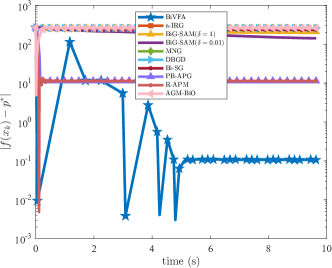
Figure 2: The performances of our methods compared with other methods in IEP.

Figure 2 illustrates that our method outperforms other approaches. Specifically, our method achieves the best performance concerning the lower-level objective, with PB-APG and R-APM ranking second. Regarding the upper-level objective, our method also excels. These findings confirm the superior complexity results of our method, as shown in Table 1.

6.2 Linear Regression Problem (LRP)

In the second experiment, we address a linear regression problem aimed at determining a parameter vector $\mathbf{x}\in\mathbb{R}^{n}$ that minimizes the training loss $\ell_{{\rm tr}}(\mathbf{x})=\frac{1}{2}\|\mathbf{A}_{{\rm tr}}\mathbf{x}-\mathbf{b}_{{\rm tr}}\|^{2}$ with the training dataset $\mathbf{A}_{{\rm tr}}$ and $\mathbf{b}_{{\rm tr}}$ [3, 47, 16, 33, 39, 27, 58, 11]. It is evident that the linear regression problem may exhibit multiple global minima without explicit regularization. Then, we consider a secondary objective, i.e., the loss on a validation dataset $\mathbf{A}_{{\rm val}}$ and $\mathbf{b}_{{\rm val}}$ [27, 11], aiding in the selection of the optimal minimizer for the training loss. Additionally, to conserve storage space, we incorporate an $\ell_{1}$-norm regularization term, resulting in the following simple bilevel problem:

$$\begin{array}[]{lcl}&\min\limits_{\mathbf{x}\in\mathbb{R}^{n}}&\frac{1}{2}\|\mathbf{A}_{{\rm val}}\mathbf{x}-\mathbf{b}_{{\rm val}}\|^{2}+\|\mathbf{x}\|_{1}\\ &{\rm{s.t.}}&\mathbf{x}\in\operatorname*{arg\,min}\limits_{\mathbf{z}\in\mathbb{R}^{n}}\frac{1}{2}\|\mathbf{A}_{{\rm tr}}\mathbf{x}-\mathbf{b}_{{\rm tr}}\|^{2}.\end{array}$$ (52)

Here, we conduct an experiment using the YearPredictionMSD dataset, which contains information on $515,345$ songs, with a release year from $1992$ to $2011$. Each song in the dataset is associated with its release year and 90 additional attributes. We randomly select a sample of $1,000$ songs from the dataset, and denote the feature matrix and the release years by $\mathbf{A}$ and $\mathbf{b}$, respectively. Following [39], we apply min-max scaling to the data and augment $\mathbf{A}$ with an intercept and 90 co-linear attributes. The dataset is split into a training set $(\mathbf{A}_{{\rm tr}},\mathbf{b}_{{\rm tr}})$ comprising $60\%$ of $\mathbf{A}$ and $\mathbf{b}$, and a validation set $(\mathbf{A}_{{\rm val}},\mathbf{b}_{{\rm val}})$ with the remaining $40\%$. To simulate real-world noise, we introduced noise sampled from a normal distribution with $\mu=0$ and $\sigma=0.2$ into the validation set $(\mathbf{A}_{{\rm val}},\mathbf{b}_{{\rm val}})$. In this experiment, we compare our method with a-IRG [28], PB-APG [13] and R-APM [11]. Similarly, for benchmarking purposes, we employ the MATLAB functions lsqminnorm and fmincon to solve the unconstrained lower-level problem and Problem (52) to obtain the optimal values $g^{*}$ and $p^{*}$, respectively.

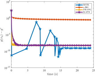
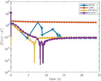
Figure 3: The performances of our methods compared with other methods in LRP.

Figure 3 illustrates that our method outperforms other methods for the lower-level objective and performs comparably to PB-APG and R-APM for the upper-level objective, demonstrating the effectiveness of our proposed approach. Furthermore, our method surpasses a-IRG in the upper-level objective, highlighting its superior efficiency. These findings are consistent with those from the first experiment.

6.3 Linear Regression Problem with Ball Constraints (LRPBC)

In the third experiment, we examine a scenario where both the upper- and lower-level objectives include a non-smooth term. Specifically, the solution to the upper-level objective is constrained within $C_{1}=\{\mathbf{x}:\|\mathbf{x}\|_{2}\leq 5\}$, and the solution to the lower-level objective is constrained within $C_{2}=\{\mathbf{x}:\|\mathbf{x}\|_{1}\leq 10\}$. Additionally, we perform the linear regression problem described in Section 6.2 without the $\ell_{1}$-norm regularization term in the upper-level objective, while keeping the other settings unchanged. Consequently, we need to solve the following simple bilevel problem:

$$\begin{array}[]{lcl}&\min\limits_{\mathbf{x}\in\mathbb{R}^{n}}&\frac{1}{2}\|\mathbf{A}_{{\rm val}}\mathbf{x}-\mathbf{b}_{{\rm val}}\|^{2}+{\rm I}_{C_{1}}\\ &{\rm{s.t.}}&\mathbf{x}\in\operatorname*{arg\,min}\limits_{\mathbf{z}\in\mathbb{R}^{n}}\frac{1}{2}\|\mathbf{A}_{{\rm tr}}\mathbf{x}-\mathbf{b}_{{\rm tr}}\|^{2}+{\rm I}_{C_{2}}.\end{array}$$ (53)

Here, we compare our method with a-IRG [28], Bi-SG [39], PB-APG [13], and R-APM [11]. For benchmarking purposes, we use the Greedy FISTA algorithm [34] and the MATLAB function fmincon to solve the unconstrained lower-level problem and Problem (53), obtaining the optimal values $g^{*}$ and $p^{*}$, respectively. Additionally, the proximal mapping of $g_{2}+zf_{2}$ at $\mathbf{x}$ involves projecting onto the intersection of the $\ell_{1}$- and $\ell_{2}$-norm balls. We employ the method proposed by [36] to compute this projection.

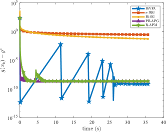
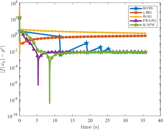
Figure 4: The performances of our methods compared with other methods in LRPBC.

Figure 4 demonstrates that our method outperforms other methods in the upper-level objective and performs comparably to PB-APG and R-APM for the lower-level objective. Furthermore, our method surpasses a-IRG and Bi-SG. These findings are consistent with the results of the first and second experiments.

7 Conclusion

This paper addresses the problem of minimizing a composite convex upper-level objective within the optimal solution set of a composite convex lower-level problem. We demonstrate that solving the simple bilevel problem is equivalent to identifying the left-most root of a nonlinear equation. Subsequently, we employ a bisection method to solve this nonlinear equation. By introducing a novel dual approach for solving the subproblem, our proposed algorithm can produce an $(\epsilon,\epsilon)$-optimal solution with near-optimal complexity results for both the upper- and lower-level problems under weak assumptions. Notably, this near-optimal rate aligns with the optimal rate observed in unconstrained smooth or composite optimization when omitting the logarithmic terms. Numerical experiments also demonstrate the superior performance of our method compared to state-of-the-art approaches.

References

- Amini and Yousefian [2019] Mostafa Amini and Farzad Yousefian. An iterative regularized incremental projected subgradient method for a class of bilevel optimization problems. In 2019 American Control Conference (ACC), pages 4069–4074. IEEE, 2019.
- Beck [2017] Amir Beck. First-order methods in optimization. SIAM, 2017.
- Beck and Sabach [2014] Amir Beck and Shoham Sabach. A first order method for finding minimal norm-like solutions of convex optimization problems. Mathematical Programming, 147(1-2):25–46, 2014.
- Beck and Teboulle [2009] Amir Beck and Marc Teboulle. A fast iterative shrinkage-thresholding algorithm for linear inverse problems. SIAM journal on imaging sciences, 2(1):183–202, 2009.
- Bertinetto et al. [2019] L Bertinetto, J Henriques, P Torr, and A Vedaldi. Meta-learning with differentiable closed-form solvers. In International Conference on Learning Representations (ICLR), 2019. International Conference on Learning Representations, 2019.
- Bertsekas [1997] Dimitri P Bertsekas. Nonlinear programming. Journal of the Operational Research Society, 48(3):334–334, 1997.
- Bigi et al. [2022] Giancarlo Bigi, Lorenzo Lampariello, and Simone Sagratella. Combining approximation and exact penalty in hierarchical programming. Optimization, 71(8):2403–2419, 2022.
- Bishop et al. [2020] Nicholas Bishop, Long Tran-Thanh, and Enrico Gerding. Optimal learning from verified training data. Advances in Neural Information Processing Systems, 33:9520–9529, 2020.
- Bonnans and Shapiro [2013] J Frédéric Bonnans and Alexander Shapiro. Perturbation analysis of optimization problems. Springer Science & Business Media, 2013.
- Boob et al. [2023] Digvijay Boob, Qi Deng, and Guanghui Lan. Stochastic first-order methods for convex and nonconvex functional constrained optimization. Mathematical Programming, 197(1):215–279, 2023.
- Cao et al. [2024] Jincheng Cao, Ruichen Jiang, Erfan Yazdandoost Hamedani, and Aryan Mokhtari. An accelerated gradient method for simple bilevel optimization with convex lower-level problem. arXiv preprint arXiv:2402.08097, 2024.
- Chambolle and Dossal [2015] Antonin Chambolle and Ch Dossal. On the convergence of the iterates of the “fast iterative shrinkage/thresholding algorithm”. Journal of Optimization theory and Applications, 166:968–982, 2015.
- Chen et al. [2024] Pengyu Chen, Xu Shi, Rujun Jiang, and Jiulin Wang. Penalty-based methods for simple bilevel optimization under h”o lderian error bounds. arXiv preprint arXiv:2402.02155, 2024.
- Dempe [2002] Stephan Dempe. Foundations of bilevel programming. Springer Science & Business Media, 2002.
- Dempe and Zemkoho [2020] Stephan Dempe and Alain Zemkoho. Bilevel optimization. In Springer optimization and its applications, volume 161. Springer, 2020.
- Dempe et al. [2021] Stephan Dempe, Nguyen Dinh, Joydeep Dutta, and Tanushree Pandit. Simple bilevel programming and extensions. Mathematical Programming, 188:227–253, 2021.
- Dempe et al. [2010] Stephen Dempe, Nguyen Dinh, and Joydeep Dutta. Optimality conditions for a simple convex bilevel programming problem. Variational Analysis and Generalized Differentiation in Optimization and Control: In Honor of Boris S. Mordukhovich, pages 149–161, 2010.
- Doron and Shtern [2023] Lior Doron and Shimrit Shtern. Methodology and first-order algorithms for solving nonsmooth and non-strongly convex bilevel optimization problems. Mathematical Programming, 201:521–558, 2023.
- Dutta and Pandit [2020] Joydeep Dutta and Tanushree Pandit. Algorithms for simple bilevel programming. Bilevel Optimization: Advances and Next Challenges, pages 253–291, 2020.
- Facchinei et al. [2014] Francisco Facchinei, Jong-Shi Pang, Gesualdo Scutari, and Lorenzo Lampariello. Vi-constrained hemivariational inequalities: distributed algorithms and power control in ad-hoc networks. Mathematical Programming, 145(1-2):59–96, 2014.
- Feurer and Hutter [2019] Matthias Feurer and Frank Hutter. Hyperparameter optimization. Automated machine learning: Methods, systems, challenges, pages 3–33, 2019.
- Franceschi et al. [2018] Luca Franceschi, Paolo Frasconi, Saverio Salzo, Riccardo Grazzi, and Massimiliano Pontil. Bilevel programming for hyperparameter optimization and meta-learning. In International conference on machine learning, pages 1568–1577. PMLR, 2018.
- Giang-Tran et al. [2023] Khanh-Hung Giang-Tran, Nam Ho-Nguyen, and Dabeen Lee. Projection-free methods for solving convex bilevel optimization problems. arXiv preprint arXiv:2311.09738, 2023.
- Gong and Liu [2021] Chengyue Gong and Xingchao Liu. Bi-objective trade-off with dynamic barrier gradient descent. NeurIPS 2021, 2021.
- Helou and Simões [2017] Elias S Helou and Lucas EA Simões. -subgradient algorithms for bilevel convex optimization. Inverse Problems, 33(5):055020, 2017.
- Hong et al. [2023] Mingyi Hong, Hoi-To Wai, Zhaoran Wang, and Zhuoran Yang. A two-timescale stochastic algorithm framework for bilevel optimization: Complexity analysis and application to actor-critic. SIAM Journal on Optimization, 33(1):147–180, 2023.
- Jiang et al. [2023] Ruichen Jiang, Nazanin Abolfazli, Aryan Mokhtari, and Erfan Yazdandoost Hamedani. A conditional gradient-based method for simple bilevel optimization with convex lower-level problem. In International Conference on Artificial Intelligence and Statistics, pages 10305–10323. PMLR, 2023.
- Kaushik and Yousefian [2021] Harshal D. Kaushik and Farzad Yousefian. A method with convergence rates for optimization problems with variational inequality constraints. SIAM Journal on Optimization, 31(3):2171–2198, 2021.
- Kissel et al. [2020] Matthias Kissel, Martin Gottwald, and Klaus Diepold. Neural network training with safe regularization in the null space of batch activations. In Artificial Neural Networks and Machine Learning–ICANN 2020: 29th International Conference on Artificial Neural Networks, Bratislava, Slovakia, September 15–18, 2020, Proceedings, Part II 29, pages 217–228. Springer, 2020.
- Kochenderfer [2019] MJ Kochenderfer. Algorithms for Optimization. The MIT Press Cambridge, 2019.
- Konda and Tsitsiklis [1999] Vijay Konda and John Tsitsiklis. Actor-critic algorithms. Advances in neural information processing systems, 12, 1999.
- Lampariello et al. [2022] Lorenzo Lampariello, Gianluca Priori, and Simone Sagratella. On the solution of monotone nested variational inequalities. Mathematical Methods of Operations Research, 96(3):421–446, 2022.
- Latafat et al. [2023] Puya Latafat, Andreas Themelis, Silvia Villa, and Panagiotis Patrinos. Adabim: An adaptive proximal gradient method for structured convex bilevel optimization. arXiv preprint arXiv:2305.03559, 2023.
- Liang et al. [2022] Jingwei Liang, Tao Luo, and Carola-Bibiane Schonlieb. Improving “fast iterative shrinkage-thresholding algorithm”: faster, smarter, and greedier. SIAM Journal on Scientific Computing, 44(3):A1069–A1091, 2022.
- Lin and Xiao [2014] Qihang Lin and Lin Xiao. An adaptive accelerated proximal gradient method and its homotopy continuation for sparse optimization. In International Conference on Machine Learning, pages 73–81. PMLR, 2014.
- Liu et al. [2020] Hongying Liu, Hao Wang, and Mengmeng Song. Projections onto the intersection of a one-norm ball or sphere and a two-norm ball or sphere. Journal of Optimization Theory and Applications, 187:520–534, 2020.
- Malitsky [2017] Yura Malitsky. Chambolle-pock and tseng’s methods: relationship and extension to the bilevel optimization. arXiv preprint arXiv:1706.02602, 2017.
- Mei and Zhu [2015] Shike Mei and Xiaojin Zhu. Using machine teaching to identify optimal training-set attacks on machine learners. In Proceedings of the Twenty-Ninth AAAI Conference on Artificial Intelligence, pages 2871–2877, 2015.
- Merchav and Sabach [2023] Roey Merchav and Shoham Sabach. Convex bi-level optimization problems with nonsmooth outer objective function. SIAM Journal on Optimization, 33(4):3114–3142, 2023.
- Muñoz-González et al. [2017] Luis Muñoz-González, Battista Biggio, Ambra Demontis, Andrea Paudice, Vasin Wongrassamee, Emil C Lupu, and Fabio Roli. Towards poisoning of deep learning algorithms with back-gradient optimization. In Proceedings of the 10th ACM workshop on artificial intelligence and security, pages 27–38, 2017.
- Nemirovsky and Yudin [1983] Arkadij Semenovič Nemirovsky and David Borisovich Yudin. Problem complexity and method efficiency in optimization. Wiley, 1983.
- Nesterov [1983] Yurii Nesterov. A method for solving the convex programming problem with convergence rate o (1/k2). In Dokl akad nauk Sssr, volume 269, page 543, 1983.
- Pedregosa [2016] Fabian Pedregosa. Hyperparameter optimization with approximate gradient. In International conference on machine learning, pages 737–746. PMLR, 2016.
- Phillips [1962] David L Phillips. A technique for the numerical solution of certain integral equations of the first kind. Journal of the ACM (JACM), 9(1):84–97, 1962.
- Rajeswaran et al. [2019] Aravind Rajeswaran, Chelsea Finn, Sham M Kakade, and Sergey Levine. Meta-learning with implicit gradients. Advances in neural information processing systems, 32, 2019.
- Rockafellar [1970] R.T. Rockafellar. Convex Analysis. Princeton University Press, Princeton, 1970.
- Sabach and Shtern [2017] Shoham Sabach and Shimrit Shtern. A first order method for solving convex bilevel optimization problems. SIAM Journal on Optimization, 27(2):640–660, 2017.
- Samadi et al. [2023] Sepideh Samadi, Daniel Burbano, and Farzad Yousefian. Achieving optimal complexity guarantees for a class of bilevel convex optimization problems. arXiv preprint arXiv:2310.12247, 2023.
- Shaban et al. [2019] Amirreza Shaban, Ching-An Cheng, Nathan Hatch, and Byron Boots. Truncated back-propagation for bilevel optimization. In The 22nd International Conference on Artificial Intelligence and Statistics, pages 1723–1732. PMLR, 2019.
- Shehu et al. [2021] Yekini Shehu, Phan Tu Vuong, and Alain Zemkoho. An inertial extrapolation method for convex simple bilevel optimization. Optimization Methods and Software, 36(1):1–19, 2021.
- Shen et al. [2023] Lingqing Shen, Nam Ho-Nguyen, and Fatma Kılınç-Karzan. An online convex optimization-based framework for convex bilevel optimization. Mathematical Programming, 198(2):1519–1582, 2023.
- Solodov [2007] Mikhail Solodov. An explicit descent method for bilevel convex optimization. Journal of Convex Analysis, 14(2):227, 2007.
- Studniarski and Ward [1999] Marcin Studniarski and Doug E Ward. Weak sharp minima: characterizations and sufficient conditions. SIAM Journal on Control and Optimization, 38(1):219–236, 1999.
- Tikhonov and Arsenin [1977] Andreĭ Nikolaevich Tikhonov and V. I. A. K. Arsenin. Solutions of ill-posed problems. Wiley, 1977.
- Tseng [2008] Paul Tseng. On accelerated proximal gradient methods for convex-concave optimization. submitted to SIAM Journal on Optimization, 2(3), 2008.
- Wang et al. [2021] Jiali Wang, He Chen, Rujun Jiang, Xudong Li, and Zihao Li. Fast algorithms for stackelberg prediction game with least squares loss. In International Conference on Machine Learning, pages 10708–10716. PMLR, 2021.
- Wang et al. [2022] Jiali Wang, Wen Huang, Rujun Jiang, Xudong Li, and Alex L Wang. Solving stackelberg prediction game with least squares loss via spherically constrained least squares reformulation. In International Conference on Machine Learning, pages 22665–22679. PMLR, 2022.
- Wang et al. [2024] Jiulin Wang, Xu Shi, and Rujun Jiang. Near-optimal convex simple bilevel optimization with a bisection method. In International Conference on Artificial Intelligence and Statistics, pages 2008–2016. PMLR, 2024.
- Woodworth and Srebro [2016] Blake E Woodworth and Nati Srebro. Tight complexity bounds for optimizing composite objectives. Advances in neural information processing systems, 29, 2016.
- Xu [2020] Yangyang Xu. Primal-dual stochastic gradient method for convex programs with many functional constraints. SIAM Journal on Optimization, 30(2):1664–1692, 2020.
- Xu [2022] Yangyang Xu. First-order methods for problems with o (1) functional constraints can have almost the same convergence rate as for unconstrained problems. SIAM Journal on Optimization, 32(3):1759–1790, 2022.
- Xu and Yin [2013] Yangyang Xu and Wotao Yin. A block coordinate descent method for regularized multiconvex optimization with applications to nonnegative tensor factorization and completion. SIAM Journal on imaging sciences, 6(3):1758–1789, 2013.
- Yousefian [2021] Farzad Yousefian. Bilevel distributed optimization in directed networks. In 2021 American Control Conference (ACC), pages 2230–2235. IEEE, 2021.