Event-based reconstruction of time-resolved centreline deformation of flapping flags

Abstract

High-speed imaging is central to the experimental investigation of fast phenomena, like flapping flags. Event-based cameras use new types of sensors that address typical challenges such as low illumination conditions, large data transfer, and the trade-off between increasing repetition rate and measurement duration more efficiently and at reduced costs compared to classical frame-based fast cameras. Event-based cameras output unstructured data that frame-based algorithms can not process. This paper proposes a general method to reconstruct the motion of a slender object similar to the centreline of a flapping flag from raw streams of event data. Our algorithm relies on a coarse chain-like structure that encodes the current state of the line and is updated by the occurrence of new events. The algorithm is applied to synthetic data, generated from known motions, to demonstrate that the method is accurate up to one percent of error for tip-based, shape-based, and modal decomposition metrics. Degradation of the reconstruction accuracy due to simulated defects only occurs when the defect intensities become more than two orders of magnitude larger than the values expected in experiments. The algorithm is then applied to experimental data of flapping flags, and we obtain relative errors below one percent when comparing the results with the data from laser distance sensors. The reconstruction of line deformation from event-based data is accurate and robust, and unlocks the ability to perform autonomous measurements in experimental mechanics.

Keywords: event-based camera, line tracking, high-speed imaging, flapping flags.

1 Introduction

Many phenomena in experimental mechanics are fast and require fast imaging techniques. Dynamic crack propagation [1], buckling rods [2], snap-through beams [3] or fluttering foils are fast phenomena that are characterised by time scales of the order of microsecond to millisecond. Flags and slender flexible structures that are immersed in a flow are subject to flutter, a dynamic instability [4]. Experimental studies of flags in a wind tunnel help improve our understanding and modelling of unsteady aerodynamics, with applications in energy harvesting [5], biological tissues [6, 7] and bio-inspired propulsion [8]. Fluttering flag experiments in a wind tunnel (figure 1.a) involve flapping frequencies ${f}_{\scalebox{0.65}{flapping}}$ from 1050 [9]. The flapping behaviour of flags is characterised by their time-resolved deformation for various wind speeds ${U}_{\scalebox{0.65}{$\infty$}}$ (figure 1.b).

Measuring the deformation of flapping flags with high temporal and spatial resolution is challenging and costly. Distance sensors can provide displacement signals with high temporal resolution but only at a single spatial location (figure 1.c). Frame-based imaging captures space-resolved data at subsequent time instants, but save irrelevant or repeated information for a large portion of the pixels in the snapshots (figure 1.d). Cameras with a higher spatial resolution can typically record for a long time at low frame rates. Cameras with a higher frame rate using modern global shutter sensors are associated with lower spatial resolution and shorter recording times as the amount of data is limited by the transfer rate and size of the camera buffer [10]. Such high frame rate cameras are expensive, and the associated high shutter speeds call for higher intensity illumination to avoid the signal-to-noise ratio to drop. Event-based cameras continuously record dynamic variations of light at the pixel level [11], creating a flow of pixel-level information in the moving areas only (figure 1.e). Event-based cameras unlock new capabilities for high spatio-temporal resolution tracking of objects, with no motion blur, and high dynamic range, at a fraction of the price [11].

The difference in the data structure between event-based and frame-based imaging calls for a paradigm shift in the development of processing algorithms. Specific applications include the tracking of objects [12, 13, 14], micro particles [15], or seeding particles for flow field measurements using particle tracking or particle image velocimetry [16, 17, 18]. Recent contributions to event-based extraction of the centreline deformation of flexible membranes [19] and seeding particles [18] still relied on pulsed illumination to generate discontinuous bursts of events. Raw data are sampled at each light pulse and processed one pulse at a time. Pulsed illumination compels the user to know a priori the typical time scales of the recorded phenomena, and duplicates static information at each pulse. Here, we present an algorithm that uses continuous illumination and leverages the full potential of event-based imaging to reconstruct the centreline deformations of a flapping flag with arbitrary time discretisation.

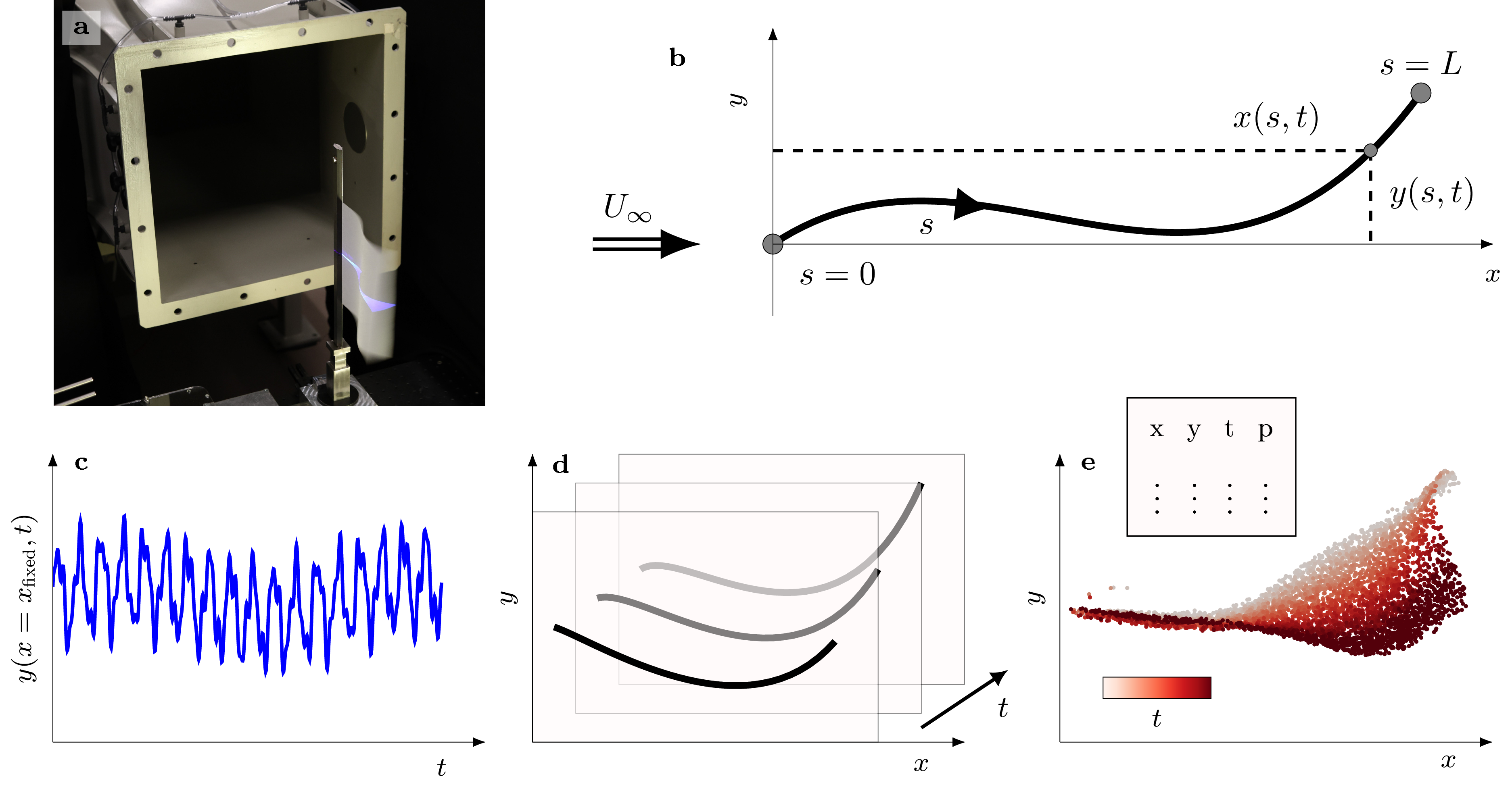
Figure 1: Example of the measurement of the centreline of a flapping flag. (a) Photograph of the flapping flag at the wind tunnel outlet. The 2D motion of the centreline is lit up in purple and recorded with the event-based camera. (b) Coordinates $x(s,t)$ and $y(s,t)$ describe the 2D motion of the centreline along the curvilinear abscissa $s$ at time $t$. The root ($s=0$) is fixed and the tip ($s=L$) is free to move. The free-stream flows along the $x$-axis with velocity ${U}_{\scalebox{0.65}{$\infty$}}$. The information used to reconstruct the centreline motion can be formatted as (c) a 1D transverse displacement at a fixed downstream position $x={x}_{\scalebox{0.65}{fixed}}$, (d) a series of instantaneous snapshots of the illuminated centreline or (e) a table of individual events plotted as a cloud coloured by time.

Figure 2: (a) The event-based camera outputs a cloud of events following the shape of the centreline motion in the $(x,y,t)$ space. (b) The coarse structure that encodes the current state of the centreline consists of links and joints. The relative location of joint ${r}_{\scalebox{0.65}{k}}$ with respect to joint ${r}_{\scalebox{0.65}{k-1}}$ is given by the polar coordinates $({r}_{\scalebox{0.65}{k}},{\theta}_{\scalebox{0.65}{k}})$. The coloured arc represents the search area around the current joint position to update the coordinates in the next time step. (c) Two blocs of events are projected on the $(x,y)$ plane and overlaid with the reconstructed line and joints positions. The colour indicates the time of the events for two blocks of duration $\tau/T=$6.2\text{\times}{10}^{-2}$$ at different moments in time. (d) The same events as in (c) are shown, coloured by the search area surrounding individual joints.

2 Method

Event-based cameras record changes in intensity at the pixel level. Here, we consider a flapping flag in a uniform flow that is imaged using an event-based camera to measure the centreline deformation of the flag in time (figure 1). The centreline is illuminated by a laser sheet normal to the flag that intersects the flag at mid-height. An event-based camera records the reflections of the laser sheet on the flag from above. If the flag is stable and remains still, the centreline does not move in the field of view. The light intensity at each pixel stays constant over time and no events are generated. When the flag flaps, the position of the illuminated centreline moves in the field of view. Photoreceptors undergo light intensity transitions when the centreline reflections pass them. Individual pixel events are generated at the precise time and location in the field of view corresponding to the locations where the centreline passes by. The list of events can be represented as a cloud indicating the changes in centreline deformation in space and time (figure 2.a). Each event is described by a spatial position ${x}_{\scalebox{0.65}{evs}}$ and ${y}_{\scalebox{0.65}{evs}}$, a time stamp ${t}_{\scalebox{0.65}{evs}}$ and a polarity ${p}_{\scalebox{0.65}{evs}}=1$ or $0$ for increasing or decreasing brightness, respectively. This data structure is spatially sparse and provides only information about changes in the field of view. Each event indicates where something is moving, but it does not tell us which part of the flag is moving and where the rest of the flag is.

A specialised algorithm is required to convert the cloud of events into a parametrised description of the deformation of the flag’s centreline expressed by the coordinates $x(s,t)$ and $y(s,t)$ with $s$ the curvilinear abscissa and $t$ the time. The solution we propose here is an algorithm that encodes the current state of the geometry in time with a chain-like structure of ${N}_{\scalebox{0.65}{j}}$ links and joints, excluding the fixed root connection. The relative location of successive joints is defined in polar coordinates $({r}_{\scalebox{0.65}{k}},{\theta}_{\scalebox{0.65}{k}})$ (figure 2.b). The total length of the chain $L=\sum_{k=1}^{{N}_{\scalebox{0.65}{j}}}{r}_{\scalebox{0.65}{k}}$ is either kept constant for inextensible objects, or might vary in time if the material is extensible. Here, we will focus solely on inextensible flags, but the algorithm can be extended in future work to account for local stretching or compression of the material as a function of known material properties and additional measures of the local shear stress, for example. The initial distribution of the joints along the object is chosen to be equidistant here. Alternative non-equidistant distributions can be selected if desirable. The variations of ${\theta}_{\scalebox{0.65}{k}}$ along the chain describe the line curvature.

To update the chain coordinates, we consider events during an update interval of $\tau$ centered around the current processing time $t$ (figure 2.c). Events with time stamps between $t-\tau/2$ and $t+\tau/2$ are considered to define the shape at time $t$. These events are then spatially clustered starting from the root to successively update the location of the joints from the root to the tip of the flag (figure 2.d). For each joint $k$, we define an arc-shaped spatial search area as indicated in figure 2.b. Events are within the search area if their distance from the previous joint $k-1$ lies between $(1-\alpha){r}_{\scalebox{0.65}{k}}$ and $(1+\alpha){r}_{\scalebox{0.65}{k}}$ with $\alpha$ the search radius parameter, which is a scalar value between $01$ ($\alpha=0.6$ in figure 2.d). The updated location of joint $k$, ${\theta}_{\scalebox{0.65}{k}}$, is then determined by the average angle with respect to joint $k-1$ of all the events with a timestamp within the update interval and a spatial location in the search area. This process is repeated for all successive joints up to $k={N}_{\scalebox{0.65}{j}}$ for a selected time instant $t$ to obtain $({r}_{\scalebox{0.65}{k}},{\theta}_{\scalebox{0.65}{k}})$ pairs for each link. The $({r}_{\scalebox{0.65}{k}},{\theta}_{\scalebox{0.65}{k}})$ pairs are then converted to Cartesian coordinates $({x}_{\scalebox{0.65}{k}},{y}_{\scalebox{0.65}{k}})$. To smoothen this discrete joint-based centreline deformation, we replaced the straight links between joints by piecewise polynomials using the modified Akima cubic Hermite interpolation in Matlab with a final spatial curvilinear discretisation of $\textrm{d}s$. The interpolation increases the length of the centreline beyond the flag length. This is corrected for by reducing the radial coordinate ${r}_{\scalebox{0.65}{${N}_{\scalebox{0.65}{j}}$}}$ of the tip joint while maintaining the extracted tip angle ${\theta}_{\scalebox{0.65}{${N}_{\scalebox{0.65}{j}}$}}$ until the length of the smoothened centreline matches the flag length. This entire process is repeated with a time increment $\textrm{d}t$ as long as there are new events in the stream.

The algorithm presented here uses five main user-input parameters: the number of joints ${N}_{\scalebox{0.65}{j}}$, the output spatial resolution $\textrm{d}s$, the search radius parameter $\alpha$, the processing time increment $\textrm{d}t$, and the update interval $\tau$. The number of joints ${N}_{\scalebox{0.65}{j}}$ defines the coarseness of the chain and controls the resolution of the local curvature and the spatial deformation wavelength. The number of joints should be approximately an order of magnitude larger than the number of spatial deformation wavelengths that fit in the flag length and should be further increased with increasing local curvature. The spatial curvilinear resolution $\textrm{d}s$ controls the smoothness of the resulting centreline. It should be equal to or smaller than the curvilinear distance between the joints. The search radius parameter $\alpha$ controls the size of the search area and the local spatial smoothening of the deformation. Ideally $\alpha$ should be as small as possible to reduce smoothing, but large enough such that enough events are included to reduce the random error. Values of $\alpha\geq 0.5$ generate overlap between the search areas of two successive joints. The processing time increment $\textrm{d}t$ and the update interval $\tau$ determine the temporal discretisation. Ideally, the update interval is as short as possible to increase the accuracy of the local deformation velocity, but it needs to be large enough such that enough events are included to reduce the random error. The processing time increment should preferably be smaller than the update interval ($\textrm{d}t<\tau$) to ensure continuous update of the chain-like structure in our algorithm as some events will be considered for multiple time instants and sudden jumps are avoided. If there is no temporal overlap for values of $\textrm{d}t>\tau$, some events will be ignored which can lead to large jumps between position updates that will cause the algorithm to lose track and fail.

The choice of the input parameters is a compromise between precision and robustness. The influence of the processing parameters is further discussed in the next section using a benchmark test with simulated events.

3 Benchmark of the algorithm using a simulated stream of events

In this section we test the robustness of the proposed method using synthetic data. A total of $400$ kinematics that are qualitatively similar to flapping flags are generated and exported in a video format. These kinematics consist of a sum of a travelling wave and a standing wave with a growing amplitude envelope along the flag (supplementary video S1). The frequency, wavelength and weight of both waves are randomly sampled to obtain a group of kinematics with peak-to-peak amplitudes $2A/L$ ranging from $0.0851.05$ and wavelengths $\lambda/L$ ranging from $1.53.0$. The videos of the simulated motions are converted into streams of events using the function SimulatedEventsIterator from Metavision SDK [20]. These video-to-events simulations estimate successive changes of intensity between frames to mimic the properties of an event-based camera and output a file containing a stream of events [21, 22]. We use our algorithm to reconstruct the deformation for a fixed duration of the recording corresponding to $36$ flapping periods using ${N}_{\scalebox{0.65}{j}}=10$ joints.

The results of the comparison between the obtained shape $x(s,t),y(s,t)$ with the known input reference ${x}_{\scalebox{0.65}{ref}}(s,t),{y}_{\scalebox{0.65}{ref}}(s,t)$ are presented in figure 3. To evaluate the quality of the results, we propose different metrics to quantify the error in the reconstruction of the overall flag shape and the tip motion, and a modal-decomposition-based metric to compare the flapping dynamics. The instantaneous reconstruction error of the overall shape is calculated as the root-mean-square of the difference between the reconstructed and the reference position along the curvilinear abscissa (figure 3.a):

$${\varepsilon}_{\scalebox{0.65}{RMS}}(t)=\sqrt{\frac{1}{L}\int\limits_{s=0}^{s=L}\left[x(s,t)-{x}_{\scalebox{0.65}{ref}}(s,t)\right]^{2}+\left[y(s,t)-{y}_{\scalebox{0.65}{ref}}(s,t)\right]^{2}\textrm{d}s}.$$ (1)

For each flag we take the maximum of ${\varepsilon}_{\scalebox{0.65}{RMS}}$ over time as our shape-based metric. It gives an overall indication of the quality of the instantaneous shape reconstruction. The displacement of tip of the flag plays an important role in the wake formation and the characterisation of the flapping dynamics. Therefore, we also consider a tip-based metric to evaluate our algorithm. As a tip-based metric we use the temporal root-mean-square value of the Euclidean distance $\delta(t)$ between the reconstructed location and the reference location of the tip (figure 3.b):

$$\delta(t)=\sqrt{\left[x(L,t)-{x}_{\scalebox{0.65}{ref}}(L,t)\right]^{2}+\left[y(L,t)-{y}_{\scalebox{0.65}{ref}}(L,t)\right]^{2}}\quad.$$ (2)

The final metric we use to evaluate our algorithm’s performance to reconstruct the flapping flag’s dynamics is the travelling wave index $\mathcal{I}$. The travelling wave index indicates the relative contribution of travelling waves versus standing waves to the dynamics of a flapping motion [23]. If the flapping motion is a pure standing wave, $\mathcal{I}=0$, if the motion is a pure travelling wave, $\mathcal{I}=1$. The travelling wave index is obtained using the complex orthogonal decomposition of the spatio-temporal evolution of the flag’s shape. Matching travelling wave indices between the reconstructed deformations and the input shapes indicate a reliable reconstruction of the flapping dynamics.

For all motions considered, the relative root-mean square tip displacement error ${\delta}_{\scalebox{0.65}{RMS}}/L$ ranges from 0.361.0 and the maximum shape difference $\max({\varepsilon}_{\scalebox{0.65}{RMS}}/L)$ ranges from 0.531.6 (figure 3.c). Overall, an increase in the maximum shape difference goes hand in hand with an increase of the relative tip displacement error. The tip displacement error and maximum shape difference tend to increase with increasing input wavelength $\lambda/L$. The travelling wave index reconstruction shows excellent agreement over the entire range of tested kinematics (figure 3.d) with a maximum discrepancy $|\mathcal{I}-{\mathcal{I}}_{\scalebox{0.65}{ref}}|$ below $0.025$ and an average discrepancy of $2.9\text{\times}{10}^{-3}$.These results demonstrate that the method is robust for various motions using clean data and the selected processing parameters: ${N}_{\scalebox{0.65}{j}}=10$ joints, an update interval $\tau/T=$5\text{\times}{10}^{-3}$$, overlap parameter $\alpha=0.6$ and a processing time increment equal to the update interval $\textrm{d}t=\tau$. The effect of imperfect data and different choices of processing parameters are investigated next.

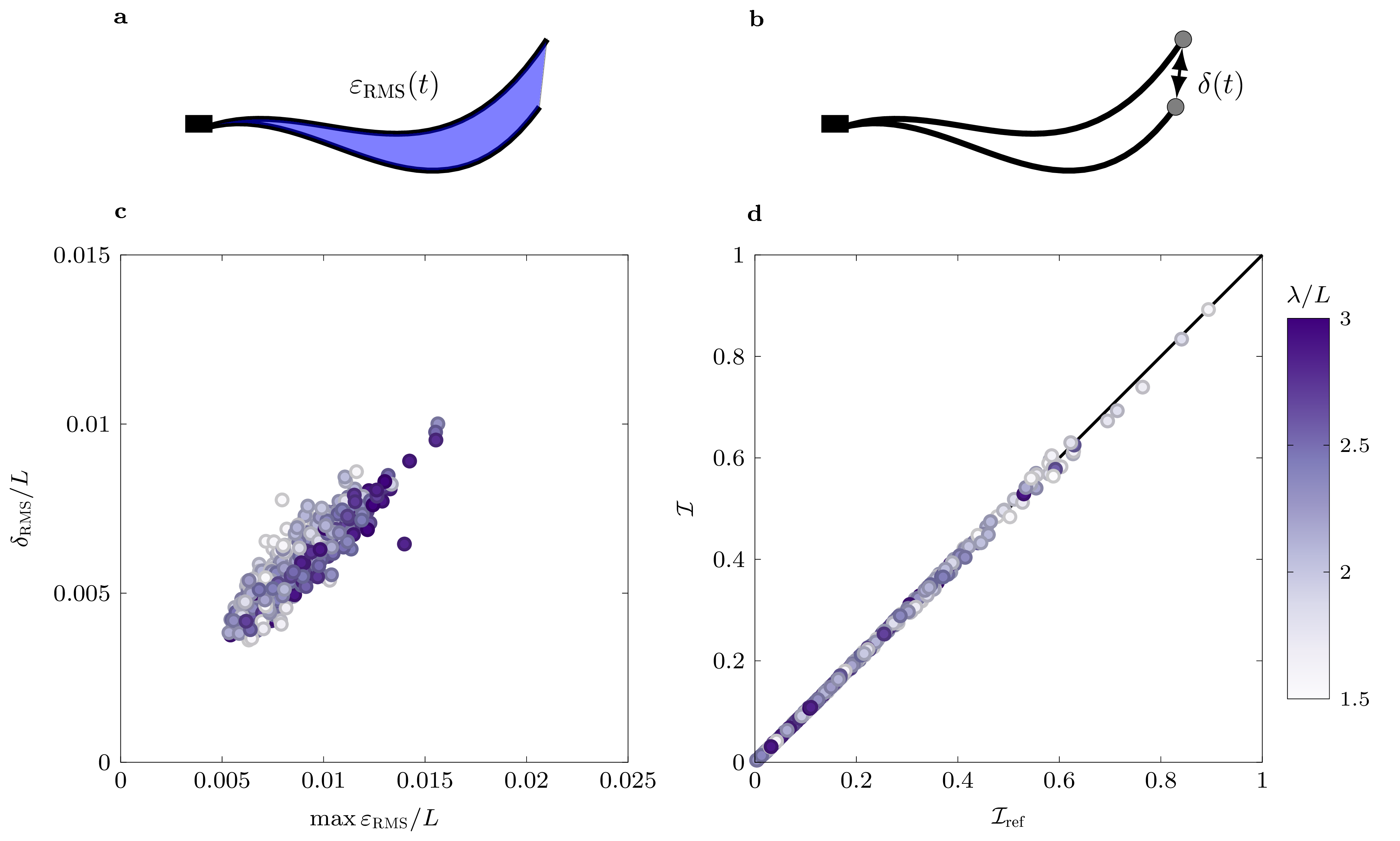
Figure 3: Quantification of the errors between the reconstructed and the exact deformation. (a) Visualisation of the shape difference determined as the root-mean-square distance along the curvilinear abscissa ${\varepsilon}_{\scalebox{0.65}{RMS}}(t)$, and (b) the tip displacement error $\delta(t)$. (c) Distribution of root-mean-square tip displacement error ${\delta}_{\scalebox{0.65}{RMS}}/L$ and maximum of the shape difference $\max{\varepsilon}_{\scalebox{0.65}{RMS}}/L$ for various kinematics tested coloured by the dimensionless wavelength $\lambda/L$. (d) Comparison of the reconstructed travelling wave index $\mathcal{I}$ with its reference value ${\mathcal{I}}_{\scalebox{0.65}{ref}}$.

3.1 Influence of hardware defects

Event-based cameras suffer from specific types of defects due to their particular hardware. Electric leakage and temperature effects cause losses of the reference light intensity at the pixel level at a typical rate of ${f}_{\scalebox{0.65}{lr}}$ [24]. Here, we tested the reconstruction accuracy and compared the results with the reference cases without event leakage (${f}_{\scalebox{0.65}{lr}}=0$). No loss of accuracy is observed for dimensionless leak rates ${f}_{\scalebox{0.65}{lr}}/{f}_{\scalebox{0.65}{flapping}}<1.2$ as the tip displacement error remains the same as in the no leakage case (figure 4.a). For higher leakage rates ${f}_{\scalebox{0.65}{lr}}/{f}_{\scalebox{0.65}{flapping}}>1.2$, the accuracy drops significantly. The tip displacement error steps up from ${\delta}_{\scalebox{0.65}{RMS}}/L=\qty{0.71}{}$ to 23 when ${f}_{\scalebox{0.65}{lr}}/{f}_{\scalebox{0.65}{flapping}}$ increases from 0 to $3.36$. The drop of accuracy originates from a severe loss of information in the cloud of events. At ${f}_{\scalebox{0.65}{lr}}/{f}_{\scalebox{0.65}{flapping}}=2.31$ (figure 4.b), most of the events have disappeared after the fourth flapping cycle (figure 4.c). Deformations do not generate any event after the first half cycle for ${f}_{\scalebox{0.65}{lr}}/{f}_{\scalebox{0.65}{flapping}}=3.89$ (figure 4.d).

The delay of first occurrence ${t}_{\scalebox{0.65}{loss}}$ of a large tip displacement error ${\delta}_{\scalebox{0.65}{RMS}}/L>0.1$ (figure 4.a) describes how many cycles can be reconstructed accurately before the tip tracking is lost, and a reset is needed. For low leak rate values ${f}_{\scalebox{0.65}{lr}}/{f}_{\scalebox{0.65}{flapping}}<1.20$, notable tip displacement errors do not occur during the first $45$ flapping cycles. When the leak ratio increases from $1.201.60$, notable tip displacement errors are already identified after $3$ flapping cycles. For a dimensionless leak rate greater than $2$, the tip tracking is lost in less than one period. Overall, the reconstruction is robust if the leak rate is lower than the characteristic flapping frequency (${f}_{\scalebox{0.65}{lr}}<{f}_{\scalebox{0.65}{flapping}}$). At room temperature, current sensors encounter ${f}_{\scalebox{0.65}{lr}}\approx\qty{0.1}{}$ [22], yielding a dimensionless leak rate ${f}_{\scalebox{0.65}{lr}}/{f}_{\scalebox{0.65}{flapping}}\approx 0.01$ for flags flapping at $\qty{10}{}$, which is well below the threshold of accuracy loss.

Ghost events due to noise can occur due to photon flux variations and electronic noise, especially at low light intensities. In the simulation, shot noise events are added to the base stream using a Poisson process with a characteristic rate of ${f}_{\scalebox{0.65}{snr}}$ [20]. The total amount of events ${N}_{\scalebox{0.65}{evs}}$ compared to the noiseless case ${N}_{\scalebox{0.65}{evs,0}}$ quantifies the proportion of meaningless data due to added noise. The tip displacement error stays below one percent for a dimensionless shot noise rate ${f}_{\scalebox{0.65}{snr}}/{f}_{\scalebox{0.65}{flapping}}<35$ (figure 4.d). At this noise rate, the events triggered by deformation only represent 51 of the total stream (${N}_{\scalebox{0.65}{evs}}/{N}_{\scalebox{0.65}{evs,0}}=1.95$). This level of noise is extreme and the characteristic shape of the event cloud seen from experimental data in figure 4.b is completely hidden in figure 4.f where ${f}_{\scalebox{0.65}{snr}}/{f}_{\scalebox{0.65}{flapping}}=10$.

The order of magnitude of the shot noise rate in current sensors is found around ${f}_{\scalebox{0.65}{snr}}\approx\qty{1}{}$ [22] and can be reduced by cooling [25] and filtering [26]. This rate of shot noise is an order of magnitude lower that the typical flapping frequency of our flags which lies around $\qty{10}{}$. For ${f}_{\scalebox{0.65}{snr}}/{f}_{\scalebox{0.65}{flapping}}\approx 0.1$, the effect of shot noise is minimal.

Figure 4: Effect of simulated defects on the reconstruction accuracy: (a) root-mean square tip displacement error ${\delta}_{\scalebox{0.65}{RMS}}/L$ ( ) for different levels of leak rate ${f}_{\scalebox{0.65}{lr}}$. The delay ${t}_{\scalebox{0.65}{loss}}$ ( ) before the first occurrence of a tip displacement error greater than $0.1L$ is plotted in terms of number of cycles. (b, c and d) Visualisation of the leaked event clouds for ${f}_{\scalebox{0.65}{lr}}/{f}_{\scalebox{0.65}{flapping}}=0,2.31,3.89$. (e) Root-mean square tip displacement error ${\delta}_{\scalebox{0.65}{RMS}}/L$ for different dimensionless shot noise rate ${f}_{\scalebox{0.65}{snr}}/{f}_{\scalebox{0.65}{flapping}}$. The total amount of events in the raw file ${N}_{\scalebox{0.65}{evs}}$ compared to the noiseless case ${N}_{\scalebox{0.65}{evs,0}}$ increases linearly with the shot noise rate: at ${f}_{\scalebox{0.65}{snr}}/{f}_{\scalebox{0.65}{flapping}}=37$, the amount of noise events equals the number of events describing the deformation (${N}_{\scalebox{0.65}{evs}}/{N}_{\scalebox{0.65}{evs,0}}=2$). (f) Visualisation of the noisy event clouds for ${f}_{\scalebox{0.65}{snr}}/{f}_{\scalebox{0.65}{flapping}}=10$.

3.2 Influence of processing parameters

The effect of the processing parameters is illustrated with one kinematic of wavelength $\lambda/L=2$. Tip-based errors decrease when increasing the number of joints up to ${N}_{\scalebox{0.65}{j}}\approx 10$ (figure 5.a) because the chain-like structure approximates the smooth deformation less coarsely. More joints allow for smoother variations in curvature along the line but gather less events per joints. The error stays low for larger number of joints. The effect of the update interval on the tip displacement error is mild for $$2\text{\times}{10}^{-3}$<\tau/T<$2\text{\times}{10}^{-2}$$ (figure 5.b). The error increases for lower and higher update intervals. At low values ($\tau/T<$2\text{\times}{10}^{-3}$$), the error increases with decreasing update interval for noisy data. Reconstruction with noiseless data maintains small errors for very low update intervals ($\tau/T\approx$2\text{\times}{10}^{-4}$$), where an average of less than 15 events are gathered per joint and update interval. In this configuration, single events can locally modify joint coordinates resulting in an increased noise sensitivity. At high values ($\tau/T>$2\text{\times}{10}^{-2}$$), large update intervals act as a moving average and smooth out the motion. Far away from these extreme cases, there exists a range of ${N}_{\scalebox{0.65}{j}}$ and $\tau$ where the precision of the reconstruction is high and stable.

Figure 5: Effect of (a) the number of joints ${N}_{\scalebox{0.65}{j}}$ and (b) update interval $\tau$ on the root-mean square tip displacement error ${\delta}_{\scalebox{0.65}{RMS}}$ with noiseless ( ) and noisy ( ) data. Shot noise level is set at ${f}_{\scalebox{0.65}{snr}}/{f}_{\scalebox{0.65}{flapping}}=20$.

4 Experimental results

The proposed algorithm is now demonstrated for experimental data. A flag made out of paper (Papeteria $\qty[mode=text]{80}{g.m^{-2}}$) is attached to a vertical pole at the outlet of an open-section wind tunnel ([product-units=power]450x450). The centreline is illuminated by a horizontal light sheet generated with a laser pointer and a Powell lens. An event-based camera (Century Arks SilkyEvCam VGA with a 35mm lens) is placed above the flag on one side and records the motion of the illuminated centreline for approximately 6s. A time-resolved laser distance sensor (Baumer OM70) measures independently the transverse displacement of the flag at $x/L=0.73$. Time synchronisation between the camera and the distance sensor is achieved with an external trigger signal. An absolute error $e(t)$ indicates the discrepancy between the distance sensor data and the reconstructed centreline from the event-based data (figure 6.a).

Comparison between the lateral displacement data from the event-based camera and the distance sensor is presented in figure 6.b. The transverse error $e(t)$ oscillates between [range-phrase= and ]01.5 of the centreline length (figure 6.c). The root-mean square distance ${\Delta}_{\scalebox{0.65}{RMS}}$ between the cloud of points and the reconstruction surface for each update interval quantifies how close the reconstruction is from the original data (figure 6.d). The cloud of points is qualitatively well captured by the reconstruction surface with ${\Delta}_{\scalebox{0.65}{RMS}}/L$ oscillating between [range-phrase= and ]0.71.2 (figure 6.e). Superimposed deformations at different time instants outline the complex motion of the centreline and the two-dimensional path of the tip (figure 6.f). The envelope depicts two necks which is consistent with the literature for this type of paper flags and flow velocities [9].

A series of deformation measurements is performed autonomously with the event-based camera (figure 6.g and h). The series of measurements go across several stages of fluid-structure interaction. For ${U}_{\scalebox{0.65}{$\infty$}}<\qty{5}{\per}$ the flag is stable and the amplitude $A/L\approx 0$. For flow velocities ranging from $\qtyrange{5}{5.5}{\per}$, the flapping amplitude first increases then plateaus before jumping up slightly at ${U}_{\scalebox{0.65}{$\infty$}}=\qty{7.5}{\per}$ (figure 6.h). Both the average distance of the reconstruction to the cloud of points and to the laser distance sensor data stay below $0.01L$ for each velocity (figure 6.g). This set-up performs the measurement loop through different velocities in less than 15 for $44$ measurement points, yielding around 4.8GB of raw data. A high-speed camera recording 8 bit images of similar resolution (640x480px) at 1000 frames per second would generate around 80GB of raw data, which is $16$ times more.

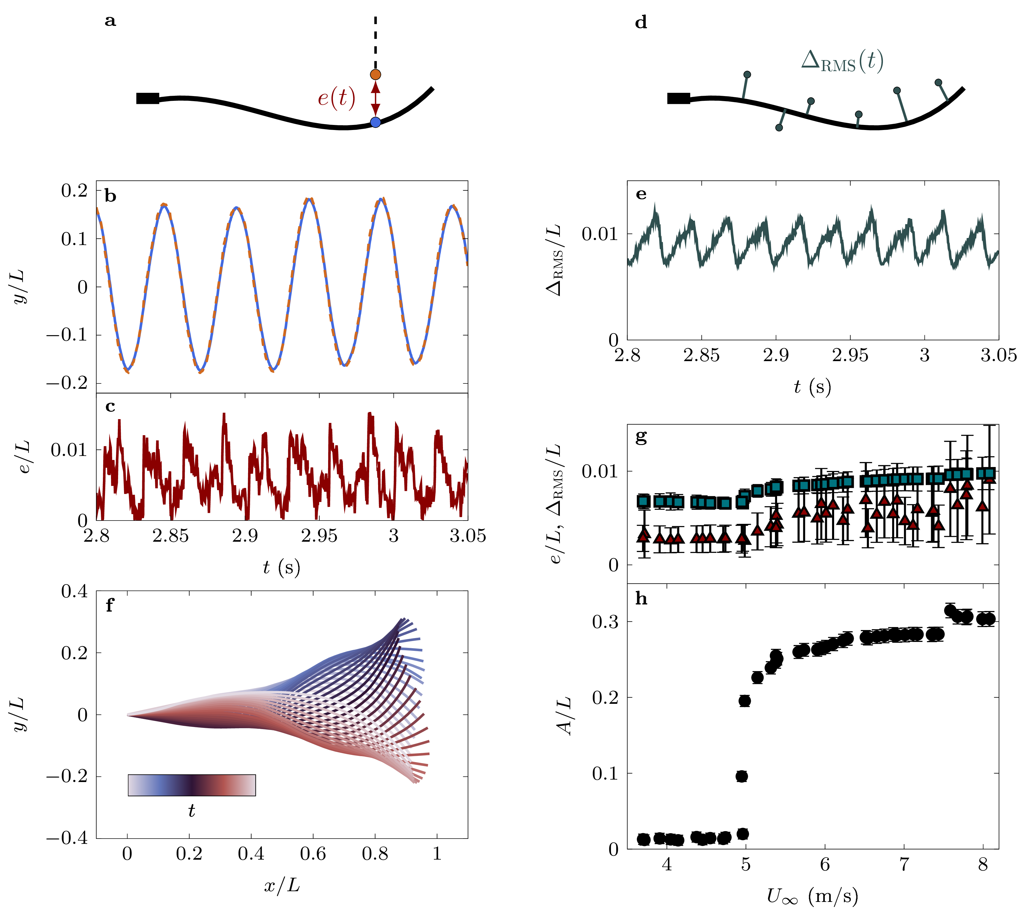
Figure 6: Accuracy metrics for experimental data are computed in terms of (a) lateral displacement $y$ at a fixed $x$ position using a laser distance sensor and (b) distance of the cloud of events to the reconstructed shape for each update interval ${\Delta}_{\scalebox{0.65}{RMS}}$. For a $L=\qty{18}{cm}$ flag at ${U}_{\scalebox{0.65}{$\infty$}}=\qty{7.2}{\per}$ flapping at $f=\qty{20.7}{}$, (c) time-resolved comparison of the lateral displacement $y/L$ obtained at $x/L=0.73$ with the event-based camera ( ) and the laser distance sensor ( ). (d) The difference of both signals defines the error $e/L$. (e) Time variation of the cloud distance ${\Delta}_{\scalebox{0.65}{RMS}}$ on the same time interval. (f) Series of reconstructed shapes coloured with time. (g) Mean and standard deviation of the error metrics ${\Delta}_{\scalebox{0.65}{RMS}}/L$ ( ) and $e/L$ ( ) and (h) tip amplitude $A/L$ ( ) for a measurement series at different inflow velocities ${U}_{\scalebox{0.65}{$\infty$}}$.

5 Conclusion

The interest of the research community in event-based cameras for fast imaging is increasing. The sensors and cameras have reached a level of maturity that makes them widely available at a price that is orders of magnitude lower than traditional high repetition rate scientific cameras. The difference in the data structure between event-based and frame-based imaging calls for the development of new processing algorithms that do not convert the streams of events back to snapshots, but instead leverage the full potential and information captured by the event detection.

Here, we presented a robust and generalisable method to reconstruct the spatio-temporal evolution of the centreline of a flapping flag from continuous raw streams of event data. Our algorithm relies on a coarse chain-like representation of the current state of the centreline and is updated by the occurrence of new events. The algorithm works with continuous illumination and leverages the full potential of event-based imaging to track fast deformations of objects tethered at a fixed location. The algorithm was applied to synthetic data and experimental data of flapping flags. The influence of hardware defects and the processing parameters was evaluated. Common hardware defects will have negligible effects for the extraction of the flapping flag dynamics. The choice of the processing parameters is a compromise between precision and robustness.

The results from synthetic data and experimental campaigns reveal high levels of accuracy for various motions, wind conditions, and levels of defects. Event-based imaging has the potential to unlock accurate tracking with high spatiotemporal resolution while reducing both storage needs and expenses by up to two orders of magnitude. When integrated in autonomous measurement loops, event-based cameras enable the exploration of large parameter spaces and accelerate data-driven discoveries in experimental mechanics.

Supplementary information

Supplementary video S1: example of a generated kinematics (reference of the motion is ms002mpt001 as described in the data set).
Data and code availability: The raw experimental data, the parameters and scripts to generate the simulation data, process the streams of events and post-process the results to obtain the figures will be shared in Zenodo after review and before submission of a revised manuscript.

References

References

- [1] Freund L B 1998 Dynamic fracture mechanics (Cambridge university press)
- [2] Gladden J R, Handzy N Z, Belmonte A and Villermaux E 2005 Physical Review Letters 94 035503 publisher: American Physical Society URL https://link.aps.org/doi/10.1103/PhysRevLett.94.035503
- [3] Gomez M, Moulton D E and Vella D 2017 Nature Physics 13 142–145 ISSN 1745-2481 number: 2 Publisher: Nature Publishing Group URL https://www.nature.com/articles/nphys3915
- [4] Yu Y, Liu Y and Amandolese X 2019 Applied Mechanics Reviews 71 ISSN 0003-6900 URL https://doi.org/10.1115/1.4042446
- [5] Eugeni M, Elahi H, Fune F, Lampani L, Mastroddi F, Romano G P and Gaudenzi P 2020 Aerospace Science and Technology 97 105634 ISSN 1270-9638 URL https://www.sciencedirect.com/science/article/pii/S127096381932824X
- [6] Aurégan Y and Depollier C 1995 Journal of Sound and Vibration 188 39–53 ISSN 0022-460X URL https://www.sciencedirect.com/science/article/pii/S0022460X85705779
- [7] Johnson E L, Rajanna M R, Yang C H and Hsu M C 2022 Forces in Mechanics 6 100053 ISSN 2666-3597 URL https://www.sciencedirect.com/science/article/pii/S2666359721000445
- [8] Müller U K 2003 Science 302 1511–1512 publisher: American Association for the Advancement of Science URL https://www.science.org/doi/full/10.1126/science.1092367
- [9] Virot E, Amandolese X and Hémon P 2013 Journal of Fluids and Structures 43 385–401 ISSN 0889-9746 URL https://www.sciencedirect.com/science/article/pii/S0889974613001977
- [10] Raffel M, Willert C E, Scarano F, Kähler C J, Wereley S T and Kompenhans J 2018 Recording Techniques for PIV Particle Image Velocimetry: A Practical Guide ed Raffel M, Willert C E, Scarano F, Kähler C J, Wereley S T and Kompenhans J (Cham: Springer International Publishing) pp 113–127 ISBN 978-3-319-68852-7 URL https://doi.org/10.1007/978-3-319-68852-7_3
- [11] Gallego G, Delbrück T, Orchard G, Bartolozzi C, Taba B, Censi A, Leutenegger S, Davison A J, Conradt J, Daniilidis K and Scaramuzza D 2022 IEEE Transactions on Pattern Analysis and Machine Intelligence 44 154–180 ISSN 1939-3539 conference Name: IEEE Transactions on Pattern Analysis and Machine Intelligence URL https://ieeexplore.ieee.org/document/9138762
- [12] Litzenberger M, Posch C, Bauer D, Belbachir A, Schon P, Kohn B and Garn H 2006 Embedded Vision System for Real-Time Object Tracking using an Asynchronous Transient Vision Sensor 2006 IEEE 12th Digital Signal Processing Workshop & 4th IEEE Signal Processing Education Workshop (Teton National Park, WY, USA: IEEE) pp 173–178 ISBN 978-1-4244-0535-0 URL http://ieeexplore.ieee.org/document/4041053/
- [13] Ghosh R, Mishra A, Orchard G and Thakor N V 2014 Real-time object recognition and orientation estimation using an event-based camera and CNN 2014 IEEE Biomedical Circuits and Systems Conference (BioCAS) Proceedings pp 544–547 iSSN: 2163-4025 URL https://ieeexplore.ieee.org/abstract/document/6981783
- [14] Conradt J, Cook M, Berner R, Lichtsteiner P, Douglas R and Delbruck T 2009 A pencil balancing robot using a pair of AER dynamic vision sensors 2009 IEEE International Symposium on Circuits and Systems pp 781–784 iSSN: 2158-1525 URL https://ieeexplore.ieee.org/document/5117867
- [15] Ni Z, Pacoret C, Benosman R, Ieng S and Régnier* S 2012 Journal of Microscopy 245 236–244 ISSN 0022-2720, 1365-2818 URL https://onlinelibrary.wiley.com/doi/10.1111/j.1365-2818.2011.03565.x
- [16] Drazen D, Lichtsteiner P, Häfliger P, Delbrück T and Jensen A 2011 Experiments in Fluids 51 1465 ISSN 1432-1114 URL https://doi.org/10.1007/s00348-011-1207-y
- [17] Willert C 2022 Event-based imaging velocimetry using pulsed illumination
- [18] Willert C E and Klinner J 2022 Experiments in Fluids 63 101 ISSN 0723-4864, 1432-1114 URL https://link.springer.com/10.1007/s00348-022-03441-6
- [19] Lyu Z, Cai W and Liu Y 2024 Measurement Science and Technology 35 055302 ISSN 0957-0233 publisher: IOP Publishing URL https://dx.doi.org/10.1088/1361-6501/ad25da
- [20] Prophesee 2023 Metavision SDK v4.4.0 URL https://docs.prophesee.ai/stable/api
- [21] Gehrig D, Gehrig M, Hidalgo-Carrio J and Scaramuzza D 2020 Video to Events: Recycling Video Datasets for Event Cameras pp 3586–3595
- [22] Hu Y, Liu S C and Delbruck T 2021 v2e: From Video Frames to Realistic DVS Events pp 1312–1321 URL https://openaccess.thecvf.com/content/CVPR2021W/EventVision/html/Hu_v2e_From_Video_Frames_to_Realistic_DVS_Events_CVPRW_2021_paper.html
- [23] Feeny B F, Sternberg P W, Cronin C J and Coppola C A 2013 Journal of Computational and Nonlinear Dynamics 8 ISSN 1555-1415 URL https://doi.org/10.1115/1.4023548
- [24] Nozaki Y and Delbruck T 2017 IEEE Transactions on Electron Devices 64 3239–3245 ISSN 0018-9383, 1557-9646 URL https://ieeexplore.ieee.org/document/7962235/
- [25] Berthelon X, Chenegros G, Finateu T, Ieng S H and Benosman R 2018 IEEE Transactions on Biomedical Circuits and Systems 12 1467–1474 ISSN 1932-4545, 1940-9990 URL https://ieeexplore.ieee.org/document/8495003/
- [26] Ding S, Chen J, Wang Y, Kang Y, Song W, Cheng J and Cao Y 2023 IEEE Transactions on Multimedia 1–12 ISSN 1520-9210, 1941-0077 URL https://ieeexplore.ieee.org/document/10078400/