SynSUM – Synthetic Benchmark with Structured and Unstructured Medical Records

Abstract

We present the SynSUM benchmark, a synthetic dataset linking unstructured clinical notes to structured background variables. The dataset consists of 10,000 artificial patient records containing tabular variables (like symptoms, diagnoses and underlying conditions) and related notes describing the fictional patient encounter in the domain of respiratory diseases. The tabular portion of the data is generated through a Bayesian network, where both the causal structure between the variables and the conditional probabilities are proposed by an expert based on domain knowledge. We then prompt a large language model (GPT-4o) to generate a clinical note related to this patient encounter, describing the patient symptoms and additional context. The SynSUM dataset is primarily designed to facilitate research on clinical information extraction in the presence of tabular background variables, which can be linked through domain knowledge to concepts of interest to be extracted from the text - the symptoms, in the case of SynSUM. Secondary uses include research on the automation of clinical reasoning over both tabular data and text, causal effect estimation in the presence of tabular and/or textual confounders, and multi-modal synthetic data generation. The dataset can be downloaded from https://github.com/prabaey/SynSUM.

1 Introduction

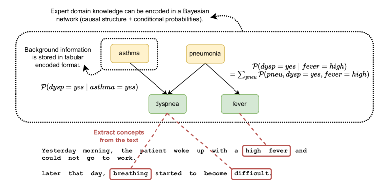
Figure 1: We have a clinical description of a patient encounter from which we want to extract some concepts, in this case the symptoms experienced by the patient. Some symptoms might be easy to extract using text-matching, like “high fever”. Other symptoms are not mentioned verbatim and are therefore harder to extract, like dyspnea. In this case, additional information on the patient, present in encoded format in the tabular portion of the EHR, together with domain knowledge, may help.
Example 1: We know that the patient has asthma. Domain knowledge tells us that the probability of experiencing dyspnea when one has asthma is 90%. This can increase the confidence of the information extraction module for the concept of dyspnea being mentioned in the text.
Example 2: We know that the patient is experiencing high fever. Domain knowledge tells us that a high fever often co-occurs with dyspnea due to their common cause, which is pneumonia. Even if we do not know that the patient has pneumonia, the probability of dyspnea being mentioned in the text increases as a result of observing high fever. If we model the joint probability of dyspnea, fever and pneumonia using a Bayesian network, we can get the exact probability of $\mathcal{P}(\text{{dyspnea = yes}}\mid\text{{fever = high}})$ by summing over the presence of pneumonia.

Electronic health records (EHRs) are a gold mine of information, containing a mix of structured tabular variables (medication, diagnosis codes, lab results…) and free unstructured text (detailed clinical notes from physicians, nurses…) (Ford et al., 2016). These EHRs form a valuable basis for training clinical decision support systems, (partially) automating essential processes in the clinical world, such as diagnosis, writing treatment plans, and more (Peiffer-Smadja et al., 2020; Mujtaba et al., 2019; Rasmy et al., 2021; Li et al., 2020; Xu et al., 2019). While large language models can help leverage the potential of the unstructured text portion of the EHR (Zhang et al., 2020; Liu et al., 2022; Huang, Altosaar, and Ranganath, 2019; Lehman and Johnson, 2023; Singhal et al., 2023; Labrak et al., 2024), these black box systems lack interpretability (Quinn et al., 2022; Zhao et al., 2024; Tian et al., 2024). In high-risk clinical applications, it can be argued that one should prefer more robust and transparent systems built on simpler, feature-based models, like regression models, decision trees, Bayesian networks, etc (Rudin, 2019; Sanchez et al., 2022; Lundberg et al., 2020). However, such models cannot directly deal with unstructured text and require tabular features as an input. For this reason, automated clinical information extraction (CIE) (Ford et al., 2016; Wang et al., 2018; Hahn and Oleynik, 2020) remains an essential tool for building large structured datasets that can serve as training data for such systems.

However, CIE remains a challenging task due to the complex nature of clinical notes. These often leave out important contextual details that an inexperienced reader would not know about, and which an automated system would need in order to correctly extract concepts from the text. Existing systems do not fully exploit the available medical domain knowledge to fill in this gap. We propose that clinical information extraction could benefit from leveraging two additional sources of information, apart from the unstructured text itself. On the one hand, we have the tabular features already encoded in the EHR, containing information on the medical history of the patient, as well as partially encoded information relating to the current visit. On the other hand, we can connect this encoded background information with the concepts we are trying to extract from the text, using medical domain knowledge. Such domain knowledge could be structured in the form of a Bayesian network. This idea is presented conceptually in Figure 1.

To put this idea into practice, we need a clinical dataset which (i) contains a mix of tabular data and unstructured text, where (ii) the tabular concepts and the concepts we aim to extract from the text can be linked through domain knowledge. While open-source datasets like MIMIC-III and MIMIC-IV contain this mix, they are too complex for the preliminary research we envision. First, the area of intensive care in which the data was collected is very extensive, making it hard to isolate a specific small-scale use-case for which the domain knowledge could be listed. Second, the portion of the dataset which is encoded into tabular features is mostly driven by billing needs, rather than completeness or accuracy, and does not contain any encoded symptoms, which are the concepts we would like to extract from the text. Third, the link between the tabular features and the concepts mentioned in the text might be inconsistent due to system design or human errors, as shown by Kwon et al. (2024). Finally, the EHRs in MIMIC are time series, adding another layer of complexity.

In this work, we build a synthetic yet sufficiently realistic dataset that addresses some of these shortcomings and allows research on the idea of incorporating domain knowledge for improved CIE in the presence of encoded tabular variables. Our dataset, called SynSUM (Synthetic Structured and Unstructured Medical records) is a self-contained set of synthetic EHRs in a primary care setting, fulfilling the following requirements:

• There is a mix of structured tabular data and unstructured text.

• The use-case in which the EHR is constructed allows us to explicitly model the domain knowledge in the form of a Bayesian network, which links the background tabular variables with the concepts expressed in the text.

• There is no time aspect, we construct the EHRs to be a static snapshot of a single patient encounter.

• The text contains additional context on some of the encoded tabular variables.

As a specific use-case, we choose the domain of respiratory diseases in primary care. Specifically, we envision the scenario where a patient visits a primary care doctor with some respiratory symptoms. The doctor notes down the patient’s symptoms in a clinical note, along with some additional context, and stores this in the electronic patient record together with the encoded diagnosis, as well as the encoded symptoms. In a realistic setting, the primary care doctor would only encode the primary complaint, rather than all symptoms. However, since we aim to build a dataset which can be used to train CIE models, where the concepts of interest are the symptoms expressed in the text, we encode all these symptoms in the artificial EHR. The tabular portion of the EHR additionally contains background information on the underlying health conditions of the patient, which may help the doctor with their diagnosis.

Section 2 describes the process of generating our SynSUM dataset of synthetic patient records in the domain of respiratory diseases. This dataset is made up of 10.000 fictional patient encounters, each represented by a set of structured tabular variables and free clinical text notes describing the encounter. Then, Section 3 runs some simple symptom predictors on our dataset, which can form a baseline for further research. Finally, Section 4 discusses the potential application of our dataset to clinical information extraction, as well as to other areas of research, while also highlighting its limitations.

2 Data generation

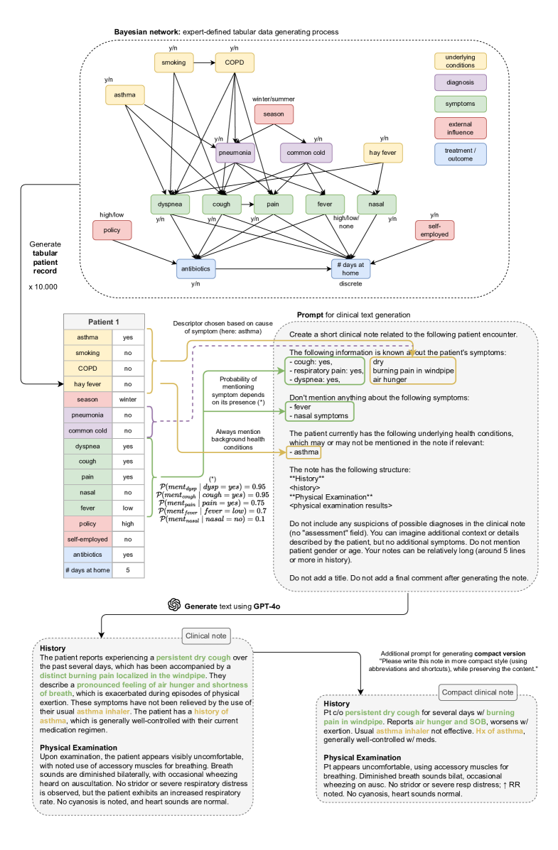
Figure 2: Overview of the full data generating process for the SynSUM dataset. First, the tabular portion of the synthetic patient record is sampled from a Bayesian network, where both the structure and the conditional probability distributions were defined by an expert. Afterwards, we construct a prompt containing information on the symptoms experienced by the patient, as well as their underlying health conditions (but no diagnoses). We ask the GPT-4o large language model to generate a fictional clinical note describing this patient encounter. Finally, we ask to generate a more challenging compact version of the note, mimicking the complexity of real clinical notes by prompting the use of abbreviations and shortcuts. We generate 10.000 of these synthetic patient records in total.

$$\mathcal{P}_{\text{{joint}}}(\text{{asthma, smoking, ..., antibio, \# days}})=\mathcal{P}(\text{{asthma}})\mathcal{P}(\text{{smoking}})\mathcal{P}(\text{{COPD}}\mid\text{{smoking}})\\ \mathcal{P}(\text{{hayf}})\mathcal{P}(\text{{season}})\mathcal{P}(\text{{pneu}}\mid\text{{asthma, COPD, season}})\mathcal{P}(\text{{cold}}\mid\text{{season}})\\ \mathcal{P}(\text{{dysp}}\mid\text{{asthma, smoking, COPD, pneu, hayf}})\mathcal{P}(\text{{cough}}\mid\text{{asthma, smoking, pneu, cold}})\\ \mathcal{P}(\text{{pain}}\mid\text{{cough, pneu, COPD, cold}})\mathcal{P}(\text{{fever}}\mid\text{{pneu, cold}})\\ \mathcal{P}(\text{{nasal}}\mid\text{{cold, hayf}})\mathcal{P}(\text{{policy}})\mathcal{P}(\text{{self-empl}})\mathcal{P}(\text{{antibio}}\mid\text{{policy, dysp, cough, pain, fever}})\\ \mathcal{P}(\text{{\#days}}\mid\text{{antibio, dysp, cough, pain, fever, nasal, self-empl}})$$ (1)

Our general methodology for generating the artificial patient records is shown in Figure 2. First, we sample a tabular patient record from an expert-defined Bayesian network. Then, we create a prompt containing the background information and symptoms available in the tabular patient record. We use this to prompt a large language model (GPT-4o) to generate a clinical note, as well as a more compact version of the same note. This process is repeated 10.000 times, leaving us with a dataset containing both the tabular patient record and two versions of the clinical note describing the patient encounter.

We now zoom in on the two major parts of this data generating process. First, Section 2.1 describes how we defined the generative process, including the Bayesian network modeling the structured tabular variables in the domain of respiratory disorders. Then, Section 2.2 dives into the clinical note generation by the large language model.

2.1 Modeling structured tabular variables with a Bayesian network

Causal structure

We asked an expert to define a Directed Acyclic Graph (DAG) which (partially) models the domain of respiratory diseases in primary care. In this DAG, a directed arrow between two variables models a causal relation between them. The full DAG is shown in the top portion of Figure 2.

Central to the model are the diagnoses of pneumonia and common cold (also known as upper respiratory tract infection), which may give rise to five symptoms. The expert also modeled some relevant underlying conditions which may render a patient more predisposed to certain diagnoses or symptoms. Based on the symptoms experienced by a patient, a primary care doctor decides whether to prescribe antibiotics or not. The presence and severity of the symptoms, as well as the prescription of antibiotics as a treatment, influence the total number of days that the patient eventually stays home as a result of illness (the outcome). Finally, there are some variables which are not clinical that exert an external influence on the diagnoses, the treatment and the outcome. Table 1 summarizes all variables and their meaning, as well as their possible values. While this model does not completely describe the real world, we do believe it to be sufficiently realistic for the purpose of generating an artificial dataset.

Name	Type	Description	Values
Asthma	underlying condition	Chronic lung disease in which the airways narrow and swell	yes/no
Smoking	underlying condition	Whether the patient is a regular smoker of tobacco	yes/no
COPD	underlying condition	Chronic Obstructive Pulmonary Disease, where airflow from the lungs is obstructed	yes/no
Hay fever	underlying condition	Allergic rhinitis, irritation of the nose caused by an allergen (e.g. pollen)	yes/no
Season	external influence	Season of the year	winter/summer
Pneumonia	diagnosis	Infection that inflames the air sacs in one or both lungs	yes/no
Common cold	diagnosis	Upper respiratory tract infection, irritation and swelling of the upper airways	yes/no
Dyspnea	symptom	Shortness of breath, the feeling of not getting enough air	yes/no
Cough	symptom	Any type of cough, no distinction between non-productive (dry) or productive (bringing up mucus or phlegm)	yes/no
Pain	symptom	Pain related to the airways or chest area	yes/no
Fever	symptom	Elevation of body temperature	high/low/none
Nasal	symptom	Nasal symptoms, such as runny nose or sneezing	yes/no
Policy	external influence	Whether the clinician has higher or lower prior inclination to prescribe antibiotics. Can be influenced by many factors, such as local policy in their general practice, their own caution towards antibiotics or level of experience.	high/low
Self-employed	external influence	Whether the patient is self-employed, rendering them less inclined to stay home from work for longer periods.	yes/no
Antibiotics	treatment	Whether any type of antibiotics are prescribed to the patient	yes/no
# Days at home	outcome	How many days the patient ends up staying home as a result of their symptoms and treatment	discrete $(0-...)$

Table 1: Description of tabular variables in our dataset.

Probability distribution

To define a data generating mechanism from which we can sample synthetic patients, we turn the DAG into a Bayesian network by defining a joint probability distribution. In a Bayesian network, this joint distribution factorizes into the product of conditional probability distributions for each variable, as shown in Equation (1). We parameterize these using four different approaches.

When the variable is discrete and has a limited number of parents, we define a conditional probability table (CPT). Each entry of the table contains the probability for a particular value of the variable, conditional on the combination of values of the parent variables. If the variable has no parents, we just define a prior probability. The probabilities in the tables were filled in by the expert based on experience, as well as demographics in Belgium and the expert’s local general practice. While we do not expect these probabilities to generalize to the global patient population as a whole, a realistic-looking distribution suffices for our use-case. We provide these tables for the variables asthma, smoking, hay fever, COPD, season, pneumonia, common cold, fever, policy and self-employed in Figure 3.

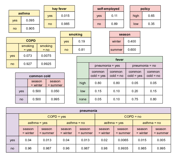
Figure 3: Conditional probability tables for the variables asthma, smoking, hay fever, COPD, season, pneumonia, common cold, fever, policy and self-employed.

For categorical variables with many parents, it becomes infeasible to manually fill in the CPT in a clinically meaningful way, because of the large number of possible combinations of parent values. This is the case for the symptoms dyspnea, cough, pain and nasal in our Bayesian network. To circumvent this problem, one can use a Noisy-OR distribution (Koller and Friedman, 2009). The Noisy-OR model is commonly used to define the distribution of a variable $Y$ which depends on a set of causes $\{X_{1},\dots,X_{k}\}$. It rests on the assumption that the combined influence of the possible causes $\{X_{1},\dots,X_{k}\}$ on $Y$ is a simple combination of the influence of each $X_{i}$ on $Y$ in isolation. This is a reasonable assumption to make in the case of symptoms with multiple possible causes (parents in the Bayesian network): a symptom arises in a patient if any of its possible causes succeeds in activating the symptom through its own independent mechanism. As shown in Equation (2), the parameterization of the noisy-OR distribution rests on choosing the parameters $p_{i}$, which is the probability that a possible cause $X_{i}$ activates symptom $Y$. As a special case, $p_{0}$, also known as the leak probability, is the probability that symptom $Y$ is activated as the result of another unmodeled cause (ouside of all $X_{i}$’s). Note that $x_{i}$ in the equation is $1$ when the cause $X_{i}$ is present in the patient, and $0$ if not. Equations (3) through (6) define such a Noisy-OR distribution for the symptoms dyspnea, cough, pain and nasal. Note that the symptom fever is fully defined through a CPT, since the expert was able to provide intuition on all possible combinations of its two parent values, eliminating the need for a Noisy-OR distribution.

$$\operatorname{Noisy-OR}(p_{0},p_{1},\dots,p_{k})\coloneq\\ \mathcal{P}(Y=1\mid X_{1},\dots,X_{k})\\ =1-\mathcal{P}(Y=0\mid X_{1},\dots.,X_{k})\text{, with}\\ \mathcal{P}(Y=0\mid X_{1}=x_{1},\dots,X_{k}=x_{k})\\ =(1-p_{0})(1-p_{1})^{x_{1}}\dots(1-p_{k})^{x_{k}}\\ \text{and }x_{1}...x_{k}\in\{0,1\}$$ (2)

$$\mathcal{P}(\text{{dysp}}\mid\text{{asthma, smoking, COPD, hayf, pneu}})\\ =\operatorname{Noisy-OR}(p_{0}=0.05,p_{\text{{asthma}}}=0.9,p_{\text{{smoking}}}=0.3,\\ p_{\text{{COPD}}}=0.9,p_{\text{{hayf}}}=0.2,p_{\text{{pneu}}}=0.3)$$ (3)

$$\mathcal{P}(\text{{cough}}\mid\text{{asthma, smoking, COPD, pneu, cold}})\\ =\operatorname{Noisy-OR}(p_{0}=0.07,p_{\text{{asthma}}}=0.3,p_{\text{{smoking}}}=0.6,\\ p_{\text{{COPD}}}=0.4,p_{\text{{pneu}}}=0.85,p_{\text{{cold}}}=0.7)$$ (4)

$$\mathcal{P}(\text{{pain}}\mid\text{{COPD}},\text{{cough}},\text{{pneu}},\text{{cold}})\\ =\operatorname{Noisy-OR}(p_{0}=0.05,p_{\text{{COPD}}}=0.15,p_{\text{{cough}}}=0.2,\\ p_{\text{{pneu}}}=0.3,p_{\text{{cold}}}=0.1)$$ (5)

$$\mathcal{P}(\text{{nasal}}\mid\text{{hayf, cold}})\\ =NoisyOR(p_{0}=0.1,p_{\text{{hayf}}}=0.85,p_{\text{{cold}}}=0.7)$$ (6)

Whether or not to prescribe antibiotics depends on whether the clinician suspects pneumonia in the patient. Their suspicion raises with the number of symptoms present in the patient, with some symptoms weighing more than others. Once their level of suspicion reaches a certain threshold, they decide to prescribe treatment. This process can be modeled using a logistic regression model taking the symptoms dyspnea, cough, pain and fever, as well as the variable policy, as an input, as shown in Equation (7). Here, $x_{po}$ (policy) can take on the values 1 (high) or 0 (low), $x_{d}$ (dyspnea), $x_{c}$ (cough) and $x_{pa}$ (pain) can take on the value 1 (yes) or 0 (no), and $x_{f}$ (fever) can be 2 (high), 1 (low) or 0 (none). The bias of $\text{-}3$ was set based on the following constraint: if there’s no symptoms at all, and policy is low, then the probability of prescribing antibiotics (due to some other unmodeled cause) should be around 5%. Similarly, the coefficient for policy was set to fit the following constraint: if there’s no symptoms at all, and policy is high, the probability should be around 10%. All other coefficients were then chosen by the expert based on the relative importance of the symptoms when deciding to prescribe antibiotics, taking the coefficient for policy as a starting point. As a final sanity-check, we asked the expert to label a set of test cases with whether they would prescribe antibiotics or not, allowing us to compare with the probability predicted by the model. Table 2 shows these results. We see that the predictions made by the model mostly correspond well with the clinician’s intuition, confirming that the proposed coefficients make sense.

$$\mathcal{P}(\text{{antibio}}=\text{{yes}}\mid\text{{policy}}=x_{po},\text{{dysp}}=x_{d},\\ \text{{cough}}=x_{c},\text{{pain}}=x_{pa},\text{{fever}}=x_{f})\\ =\text{Sigmoid}(-3+1\times x_{po}+0.8\times x_{d}+0.665\times x_{c}\\ +0.665\times x_{pa}+0.9\times(x_{f}==1)+2.25\times(x_{f}==2)),\\ \text{with }x_{po},x_{d},x_{c},x_{pa}\in\{0,1\}\text{, and }x_{f}\in\{0,1,2\}$$ (7)

Symptoms				Antibiotics
dysp	cough	pain	fever	label	pred.
no	yes	no	high	no	0.48
no	yes	yes	high	yes	0.64
yes	yes	no	high	yes	0.67
yes	yes	yes	high	yes	0.80
yes	no	no	high	yes	0.51
no	no	yes	high	yes	0.48
no	no	no	high	no	0.32
no	no	no	low	no	0.11
no	yes	no	low	no	0.19
yes	yes	no	low	no	0.35
no	yes	yes	low	no	0.31
yes	yes	yes	low	yes	0.51
yes	yes	yes	none	yes	0.30
yes	no	yes	none	no	0.18
yes	yes	no	none	no	0.18
yes	no	no	none	no	0.10
no	yes	no	none	no	0.09
no	no	yes	none	no	0.09

Table 2: Test cases labeled by the expert on whether to prescribe antibiotics or not (all assume $\text{{policy}}=\text{{low}}$). “label” indicates the expert’s decision, while “pred” indicates the model’s predicted probability (based on Equation (7)).

Finally, we need to model the number of days the patient ends up staying home due to their complaints. This depends on the symptoms experienced by the patient, as well as whether they received antibiotics as a treatment. Since the outcome is discrete, with most patients staying home for a low number of days, we decided to model this using a Poisson regression. Assuming that the effect of getting treatment would be non-linear in relation to the presence or absence of the symptoms, we defined two separate Poisson models: one where no antibiotics were prescribed (Equation (8)), and one where they were prescribed (Equation (9)). Both models take the symptoms dysp, cough, pain, nasal and fever as an input, as well as the variable self-employed, and predict a mean number of days $\lambda$, which parameterizes the Poisson distribution. The coefficients for each model were tuned using gradient descent based on the train cases shown in Table 3. Like before, the expert was asked to (loosely) label these cases for how long they suspected the patient to stay home on average as a result of these symptoms. The coefficient for the variable self-employed was tuned manually, based on the assumption that being self-employed would shave some days off the predicted number, regardless of the particular symptoms experienced by the patient. As a sanity check, we compared the mean number of days predicted by the model (parameter $\lambda$ in the Poisson model) with the number of days estimated by the expert for a small test set of cases which were not seen during training. The results are shown in Table 4.

$$\mathcal{P}(\text{{\# days}}\mid\text{{dysp}}=x_{d},\text{{cough}}=x_{c},\text{{pain}}=x_{pa},\\ \text{{nasal}}=x_{n},\text{{fever}}=x_{f},\text{{self-empl}}=x_{se},\text{{antibio}}=\text{{no}})\\ =Poisson(\lambda_{0})\\ \lambda_{0}=exp(0.010+0.64\times x_{d}+0.35\times x_{c}+0.47\times x_{pa}\\ +0.011\times x_{n}+0.81\times(x_{f}==1)\\ +1.23\times(x_{f}==2)-0.5\times x_{se})\\ \text{with }x_{d},x_{c},x_{pa},x_{n},x_{se}\in\{0,1\}\text{, and }x_{f}\in\{0,1,2\}$$ (8)

$$\mathcal{P}(\text{{\# days}}\mid\text{{dysp}}=x_{d},\text{{cough}}=x_{c},\text{{pain}}=x_{pa},\\ \text{{nasal}}=x_{n},\text{{fever}}=x_{f},\text{{selfempl}}=x_{se},\text{{antibio}}=\text{{yes}})\\ =Poisson(\lambda_{1})\\ \lambda_{1}=exp(0.16+0.51\times x_{d}+0.42\times x_{c}+0.26\times x_{pa}\\ +0.0051\times x_{n}+0.24\times(x_{f}==1)\\ +0.57\times(x_{f}==2)-0.5\times x_{se})\\ \text{with }x_{d},x_{c},x_{pa},x_{n},x_{se}\in\{0,1\}\text{, and }x_{f}\in\{0,1,2\}$$ (9)

Symptoms					Days at home
					antibio = no		antibio = yes
dysp	cough	pain	nasal	fever	label	pred.	label	pred.
no	no	no	no	none	1.5	1	1	1.1
no	yes	no	no	high	4	4.9	3.5	3.2
no	yes	no	no	low	2	3.2	2	2.3
no	yes	yes	no	high	9	7.9	4	4.1
yes	yes	no	no	high	10	9.3	5	5.3
yes	yes	yes	no	high	14	14.9	7	6.9
no	yes	yes	no	low	5	5.2	3	2.9
yes	yes	no	no	low	6	6.1	4	3.8
yes	yes	yes	no	low	10	9.8	5	4.9
yes	yes	yes	no	none	4	4.3	3.5	3.9
no	yes	yes	no	none	2	2.3	2	2.3
yes	yes	no	no	none	3	2.7	3	3
yes	no	yes	no	none	3	3.1	3	2.5
no	no	no	yes	none	2	1	2	1.2
no	yes	no	yes	high	4	4.7	3.5	3.2
no	yes	no	yes	low	2	3.3	2	2.3
no	yes	yes	yes	high	9	8	4	4.1
yes	yes	no	yes	high	10	9.4	5	5.3
yes	yes	yes	yes	high	14	15.1	7	6.9
no	yes	yes	yes	low	5	5.2	3	3
yes	yes	no	yes	low	6	6.2	4	3.8
yes	yes	yes	yes	low	10	9.9	5	4.9
yes	yes	yes	yes	none	4	4.4	3.5	3.9
no	yes	yes	yes	none	2	2.3	2	2.3
yes	yes	no	yes	none	3	2.7	3	3
yes	no	yes	yes	none	3	3.1	3	2.6

Table 3: Train cases labeled by the expert on how many days they expect a patient to stay home on average (all assuming $\text{{self-employed}}=\text{{no}}$), with and without prescribing antibiotics. “label” indicates the expert’s estimation, “pred” indicates the model’s predicted mean number of days $\lambda$ (based on Equation (8) and (9)).

Symptoms					Days at home
					antibio = no		antibio = yes
dysp	cough	pain	nasal	fever	label	pred.	label	pred.
yes	no	no	no	high	6	6.5	3.5	3.5
no	no	yes	no	high	6	5.5	3	2.7
yes	no	yes	no	high	12	10.5	5	4.5
yes	no	no	no	low	4	4.3	3	2.5
no	no	yes	no	low	4	3.7	3	1.9
yes	no	yes	no	low	6	6.9	5	3.2

Table 4: Test cases (not part of training set) labeled by the expert on how many days they expect a patient to stay home on average (all assuming $\text{{self-employed}}=\text{{no}}$), with and without prescribing antibiotics. “label” indicates the expert’s estimation, while “pred” indicates the model’s predicted mean number of days $\lambda$ after training (based on Equations (8) and (9)).

Sampling

The joint probability distribution from Equation (1) is now fully specified. We can use this Bayesian network to randomly sample the tabular portion of a patient record top-down, starting from the root variables without parents at the top and continuing further down. Each value is sampled conditionally on the variable’s parents’ values, using the conditional distributions we have defined. We repeat this process 10.000 times, leaving us with 10.000 artificial patient records consisting of 16 tabular features.

2.2 Generating unstructured text with a large language model

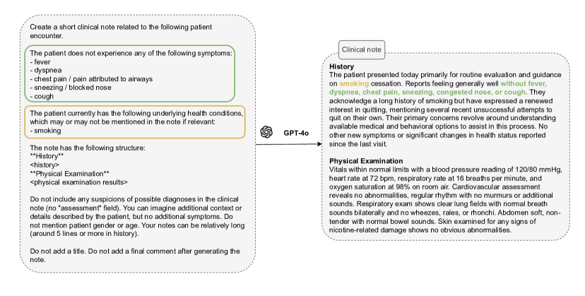
Figure 4: Example prompt and generated note for case where patient does not experience any respiratory symptoms, but does have an underlying respiratory health condition (here: smoking).

Starting from the tabular portion of the patient record, we aim to generate a text describing this fictional patient encounter. The scenario we try to mimic goes as follows. The patient goes to the primary care physician, telling them their symptoms and possible underlying conditions, along with additional context on the severity of these symptoms, when they started, among other details. The physician takes descriptive notes during this consultation, writing down the (recent) history prescribed by the patient. Then, based on the patient’s described complaints, they conduct a physical examination, writing down all findings. Both parts together then form the textual description of the patient encounter.

Our goal is to simulate this process by asking a large language model (LLM) to write a clinical note based on the information found in the tabular portion of the dataset. In this section, we describe how to build up the prompt which was used for this task. All generated prompts are generally structured like the example shown in Figure 2 (except for the special cases, see later). Only the background variables (asthma, smoking, COPD and hay fever) and symptoms (dyspnea, cough, pain, nasal and fever) may be directly mentioned in the prompt. The diagnoses pneumonia and common cold are not yet known to the clinician when they are noting down the patient history and physical examination, so these are not directly mentioned in the prompt. They can however influence the descriptors that are included next to the symptoms, as will be explained later. The treatment and outcome are left out of the prompt as well, just like the external influence variables, as all of these are not known at the time of writing the note or irrelevant to the simulated physician. Additional example prompts can be found in Appendix A.

Presence of symptoms

The first block of information in the prompt concerns the symptoms experienced by the patient. We do not list the full set of symptoms exhaustively. Even if a patient might experience a certain symptom, there is a possibility that they do not mention it to the clinician, or that the clinician does not find it noteworthy to write down. On the other hand, if a patient does not experience a symptom, it is not very likely that they will mention this to the physician, and the physician might have no reason to ask for the symptom either. We therefore ask our expert to list the probability of mentioning the symptom in a clinical note when the symptom is positive and when it is negative. Of course, this would not generalize to all physicians, but it helps to bring some variety and realism in the notes we generate. The probabilities are as follows:

• $\mathcal{P}(\text{{ment}}_{\text{{dysp}}}=\text{{yes}}\mid\text{{dysp}}=\text{{yes}})=0.95$, $\mathcal{P}(\text{{ment}}_{\text{{dysp}}}=\text{{yes}}\mid\text{{dysp}}=\text{{no}})=0.75$

• $\mathcal{P}(\text{{ment}}_{\text{{cough}}}=\text{{yes}}\mid\text{{cough}}=\text{{yes}})=0.95$, $\mathcal{P}(\text{{ment}}_{\text{{cough}}}=\text{{yes}}\mid\text{{cough}}=no)=0.9$

• $\mathcal{P}(\text{{ment}}_{\text{{pain}}}=\text{{yes}}\mid\text{{pain}}=\text{{yes}})=0.75$, $\mathcal{P}(\text{{ment}}_{\text{{pain}}}=\text{{yes}}\mid\text{{pain}}=\text{{no}})=0.3$

• $\mathcal{P}(\text{{ment}}_{\text{{fever}}}=\text{{yes}}\mid\text{{fever}}=\text{{high}})=0.95$, $\mathcal{P}(\text{{ment}}_{\text{{fever}}}=\text{{yes}}\mid\text{{fever}}=\text{{low}})=0.7$, $\mathcal{P}(\text{{ment}}_{\text{{fever}}}=\text{{yes}}\mid\text{{fever}}=\text{{none}})=0.4$

• $\mathcal{P}(\text{{ment}}_{\text{{nasal}}}=\text{{yes}}\mid\text{{nasal}}=\text{{yes}})=0.95$, $\mathcal{P}(\text{{ment}}_{\text{{nasal}}}=\text{{yes}}\mid\text{{nasal}}=\text{{no}})=0.1$

For each symptom, we randomly sample whether it is to be mentioned in the prompt, conditional on its value. As can be seen in Figure 2, we explicitly tell the model what symptoms to mention and which to steer clear from. We randomly permute the ordering of the symptoms in each prompt.

Symptom descriptors

Symptom	Cause	Descriptors
dyspnea	asthma	attack-related, at night, in episodes, wheezing, difficulty breathing in, feeling of suffocation, nighttime stuffiness, provoked by exercise, light, severe, not able to breathe properly, air hunger
	smoking	during exercise, worse in morning, mild
	COPD	chronic, worse during flare-up, worse when lying down, difficulty sleeping, air hunger
	hay fever	light, mild, stuffy feeling, all closed up
	pneumonia	light, mild, severe, no clear cause
cough	asthma	attack-related, dry
	smoking	productive, mostly in morning, during exercise, gurgling
	COPD	phlegm, sputum, gurgling, worse when lying down
	pneumonia	for over 7 days, light, mild, severe, non-productive at first and later purulent
	common cold	prickly, irritating, dry, phlegm, sputum, light, mild, severe, constant, day and night
pain	asthma	tension behind sternum
	COPD	light, mild
	cough	muscle pain, burning pain in trachea, burning pain in windpipe, scraping pain in trachea, scraping pain in windpipe
	pneumonia	light, mild, severe, localized on right side, localized on left side, associated with breathing
	common cold	burning pain in trachea, burning pain in windpipe, scraping pain in trachea, scraping pain in windpipe, light, mild

Table 5: Descriptors used in the prompt to describe each symptom when it is present in the patient. Depending on the cause(s) of the symptom (as listed in the tabular patient record), we randomly sample from a different set of descriptors.

To make the note realistic, the LLM must invent some context regarding the patient’s symptoms when writing the history portion of the note. We want this context to indirectly relate to the cause of these symptoms, as they would in a real patient encounter. For example, a cough induced by asthma would likely be momentarily and attack-related, while a cough resulting from pneumonia might be more persistent over the longer term. We therefore ask the expert to write down a list of adjectives or phrases describing each symptom, conditioned on the cause of the symptom. These descriptors can be found in Table 5. The list of possible causes for a symptom is simply the list of parents in the Bayesian network.

For each symptom which is present in the patient and selected to be mentioned in the note, we check the tabular patient record for the possible causes. For example, for the symptom cough, the possible causes are asthma, smoking, COPD, pneumonia and common cold. In the example in Figure 2, asthma is the only cause which is “on”. We therefore randomly sample a descriptor from the list of descriptors for cough in the presence of asthma, in this case the adjective “dry”. This adjective is added in the prompt. If multiple causes are “on”, we find the strongest cause, and sample from that list. The strongest cause is pneumonia, followed by common cold, followed by all other causes. If neither pneumonia nor common cold is part of the multiple causes, we simply make a bag of all descriptors associated to the causes which are “on”, and sample from that bag. In the rare event that no causes are “on”, yet a symptom is still observed (which is possible due to the leak probability in the Noisy-OR distribution), we do not add a descriptor. Note that while the diagnoses pneumonia and common cold should not be mentioned explicitly, they indirectly and subtly influence the content of the note through the descriptors, adding another realistic dimension to the content of the note.

Underlying health conditions

While the diagnoses should not be mentioned directly in the note, it is realistic to assume that the note would mention underlying health conditions the patient may have. Since these health conditions are assumed to be known up-front, as they are part of the history of the patient, they may contribute a lot to the interpretation of the symptoms by both the patient themselves and the clinician writing down the note. We therefore add them to the prompt as well, as can be seen in Figure 2. We do not force the LLM to explicitly mention these in the note, since it seems feasible that a clinician would not mention them every time. Should there be more than one underlying condition, we mention them all, randomly permuting the order in each prompt. If there are no underlying health conditions, we simply remove this part of the prompt.

Additional instructions

We tell the LLM that the note must be structured with a “History” portion and a “Physical examination” portion. While the “History” portion describes the patient’s self-reported symptoms and underlying health conditions, which are in large part dictated by the prompt, the “Physical examination” portion leaves the LLM with more freedom to imagine additional clinical examinations which were performed on the patient. As such, the “Physical examination” portion has a lot of potential for adding complexity, clinical terminology and realism to the note.

We also add some additional instructions to the prompt, asking it not to mention any suspicions of possible diagnoses. We further tell the LLM it can imagine context or details, but no additional symptoms. We noticed that if we left this part out, the LLM would sometimes mention the symptoms we specifically asked to leave out. We ask not to mention patient gender or age, because preliminary testing revealed that the LLM often used the same age and gender (34-year old woman), which could confound or bias the notes. Finally, we add that the notes may be long (around 5 lines or more), to avoid the LLM being too succinct.

Special case: no respiratory symptoms

There are 3629 out of 10.000 patients where all symptoms in the tabular record are “no”, meaning the patient does not experience any respiratory symptoms. If we used the same prompt as before, this would result in an unrealistic clinical note, since the note would simply list all symptoms the patient does not have, without giving an actual reason for the patient’s visit. Furthermore, there would be little variation in these notes. An example is shown in Figure 7 in the Appendix. For these cases, it makes more sense to assume that the patient visits for a complaint unrelated to the respiratory domain, such as back pain, stomach issues, a skin rash, etc. To generate these special cases, we use a special prompt, telling the LLM the patient does not experience any of the 5 respiratory symptoms. When the patient has at least one underlying health condition (which is the case in 239 out of 3629 special cases), we add this to the prompt in the same way as before, like the example in Figure 4. If not (i.e., for the remaining 3390 out of 3629 special cases), we tell the LLM not to mention any of those health conditions either, see the prompt in Figure 8 in the Appendix. The latter prompt asks for three clinical notes at once, encouraging the LLM to be more creative and not repeat the same scenario every time, as well as being a little more cost-effective. This is possible because of the prompt being non-specific to any of these 3390 patients. We then randomly distribute all generated texts to each tabular patient record within this subset.

Compact version

Real clinical notes can be challenging, often containing abbreviations, shortcuts and denser sentence structure. To make the notes more challenging, we asked the LLM to create such a compact version of each note through an additional prompt, as can be seen in Figure 2. Our dataset contains both the original note and the compact version of the note.

Prompting details

As a large language model, we opted for OpenAI’s GPT-4o model, using the version released in May 2024 (OpenAI, 2024). We set the temperature to 1.2 to encourage some more variation in the notes, while at the same time keeping them realistic. Before providing the case-specific prompt, we set the following system message: “You are a general practitioner, and need to summarize the patient encounter in a clinical note. Your notes are detailed and extensive.” We set the max_tokens parameter to 1000. All other parameters were kept as their default value. Generating all 10.000 notes and their compact version cost around $130$$.

3 Symptom predictor baselines

To measure the amount of information encoded in the data and set a baseline for subsequent information extraction tasks, we run various prediction models on both the tabular and textual part of the dataset. These models are trained to predict each of the five symptoms: dyspnea, cough, pain, fever and nasal.

Two of our baselines only get to see the tabular portion of the dataset at the input: Bayesian network (BN-tab) and XGBoost (XGBoost-tab). We use these models to predict each symptom in three settings, differing from one another in the set of tabular features that are taken as an input, which we call the evidence:

• $\mathcal{P}(\text{{sympt}}\mid\text{{all}})$: Predict the symptom given all other tabular features as evidence. This set includes the background, diagnoses, external influence, treatment, outcome and other symptoms.

• $\mathcal{P}(\text{{sympt}}\mid\text{{no-sympt}})$: Predict the symptom given all other tabular features as evidence, except for the other symptoms. This mimics the setting where we have tabular features available in the patient record, but have not extracted any symptoms from the text yet. This set includes the background, diagnoses, external influence, treatment and outcome variables.

• $\mathcal{P}(\text{{sympt}}\mid\text{{realistic}})$: Predict the symptom given all tabular features which would be available as evidence in a realistic setting. We do not expect policy, self-employed and #days to be recorded in any kind of realistic patient record, and therefore leave them out of this evidence set. As in the no-sympt setting, we assume that we have not extracted any tabular symptoms from the text yet. Therefore, this set includes the background, diagnoses, season and treatment variables.

Apart from the tabular-only baselines, we also train some baselines that get to see the text at the input. Our neural-text classifier takes only the text as an input (in the form of a pretrained clinical sentence embedding) and outputs the probability that a symptom is mentioned in the text. Finally, we extend this text-only baseline by concatenating a numerical representation of the tabular features to the text embedding at the input, forming the neural-text-tab baseline. Again, we do this for each of the three evidence settings outlined above. Note that this is the only model that combines both the background knowledge available in the tabular features with the unstructured text to extract, and it does so in a naive way. Future work will focus on improving the performance of this model by exploiting the relations between any of the tabular concepts, as envisioned in Figure 1.

	dyspnea	cough	pain	nasal	fever
BN-tab
- all	0.7370	0.7816	0.2386	0.7146	0.4864
- no-sympt	0.7153	0.7776	0.1312	0.7146	0.4384
- realistic	0.6698	0.7763	0.0280	0.7146	0.3594
XGBoost-tab
- all	0.6639	0.7848	0.4070	0.7130	0.4111
- no-sympt	0.6612	0.7779	0.3638	0.7146	0.4015
- realistic	0.6626	0.7798	0.3698	0.7146	0.3951
neural-text
- normal	0.9660	0.9595	0.8415	0.9602	0.9074
neural-text-tab
- normal + all	0.9526	0.9481	0.8096	0.9598	0.9113
- normal + no-sympt	0.9592	0.9530	0.8078	0.9550	0.9094
- normal + realistic	0.9544	0.9543	0.8303	0.9575	0.9033
neural-text
- compact	0.9383	0.9480	0.7828	0.9583	0.8904
neural-text-tab
- compact + all	0.9535	0.9384	0.7675	0.9566	0.9096
- compact + no-sympt	0.9363	0.9240	0.7984	0.9638	0.8760
- compact + realistic	0.9442	0.9422	0.7880	0.9606	0.8926

Table 6: F1-score obtained over the test set for each of our baseline models. The results for the text classifiers trained over the normal vs. the compact version of the notes are grouped together for readability. We report results for the mean embedding type, while results for the other embedding types can be found in Table 7. We underline the best result obtained by the tabular-only models for each symptom, while the best overall result per symptom is in shown in bold.

	dyspnea	cough	pain	nasal	fever
normal
- hist	0.9399	0.9699	0.8310	0.9538	0.9048
- phys	0.9035	0.7948	0.6871	0.9526	0.8466
- mean	0.9660	0.9595	0.8415	0.9602	0.9074
- concat	0.9635	0.9660	0.8313	0.9606	0.9086
compact
- hist	0.9353	0.9557	0.8008	0.9522	0.9148
- phys	0.8747	0.7655	0.6492	0.9544	0.8161
- mean	0.9383	0.9480	0.7828	0.9583	0.8904
- concat	0.9358	0.9443	0.7849	0.9598	0.8998

Table 7: Results for the neural-text baseline using different embedding types at the input. We report F1-score over the test set for both the normal and compact versions of the notes. The best results per symptoms and per note version is shown in bold. Figure 9 in the Appendix compares these results visually.

3.1 Models

BN-tab

We provide the causal structure in Figure 2 to the Bayesian network, and learn all parameters in the conditional probability tables (CPTs), Noisy-OR distributions, logistic regression model and Poisson regression model from the training data. In each case, we use maximum likelihood estimation to estimate the parameters and fill in a CPT. Where we don’t directly learn a CPT (for the variables dyspnea, cough, pain, nasal, antibiotics and #days), we evaluate the learned distribution for each combination of child and parent values to obtain a CPT. For more details, we refer to Appendix B.1. We then use variable elimination over the full joint distribution to evaluate the capability of the learned Bayesian network to predict each of the symptoms, taking different variables as evidence according to the 3 settings described earlier (all, no-sympt and realistic).

XGBoost-tab

We train an XGBoost classifier for each symptom in combination with each of the 3 settings, meaning each classifier has a different set of tabular features at the input. We optimize the hyperparameters separately for each combination (15 in total) using 5-fold cross-validation. For more details, we refer to Appendix B.2.

Neural-text

We train a neural classifier that takes only the text as an input and is trained to predict the probability a symptom is mentioned. We train separate classifiers for each symptom. We first split the text into sentences, and transform these into an embedding using the pretrained clinical representation model BioLORD (Remy, Demuynck, and Demeester, 2024). We explore 4 settings for turning these sentence embeddings into a single note embedding:

• hist: We average all sentence embeddings for the sentences in the “history” portion of the note.

• phys: We average all sentence embeddings for the sentences in the “physical examination” portion of the note.

• mean: To get a single representation for the full note, we take the average of the hist and phys embeddings.

• concat: Idem as previous, but now the embeddings for the two portions are concatenated.

The note embedding is then fed into a multi-layer perceptron with one hidden layer, followed by a Sigmoid activation for the symptoms dyspnea, cough, pain and nasal, and a Softmax activation with 3 outputs heads for the symptom $fever$. We optimized the parameters of each model (i.e. each combination of symptom and embedding type) using the binary or multiclass cross-entropy objective over the symptom labels. For more details, we refer to Appendix B.3.

Neural-text-tab

We extend the neural-text baseline by concatenating the mean text embeddings with the tabular variables at the input of each neural classifier. All categorical tabular variables were first transformed into a one-hot encoding, while the variable #days was preprocessed using standard scaling. We used the same architecture as the neural-text baseline (only changing the dimension of the input layer), and again trained separate classifiers for each symptom in combination with each evidence setting (all, no-sympt and realistic).

3.2 Results

We randomly split the dataset into a train and test set, using an 8000/2000 split. We use cross-validation on the train set to tune any hyperparameters, and report the final F1-score over the test set after training. We classify a symptom as positive if the predicted probability is larger than $0.5$. Since fever has three possible categories, the class with the highest predicted probability is chosen. In that case, we report the macro F1-score over all three categories.

Table 6 compares the results obtained over all baselines. The tabular-only baselines (BN-tab and XGBoost-tab) perform consistently worse than the baselines that include text (neural-text and neural-text-tab). The evidence setting where all other features are included as evidence usually performs best for the tabular-only baselines.

The neural-text-tab baseline does not perform better than the neural-text baseline when the normal notes are used. While there is little room for improvement in the dyspnea, cough and nasal classifiers, the symptoms pain and fever are harder to predict. We also note a consistent gap in performance between the normal notes and the compact notes, which can be attributed to the higher complexity of the compact notes. In that case, the neural-text-tab classifier manages to marginally improve over the neural-text classifier by including the tabular features.

Table 7 further breaks down the results for the neural-text classifier over the different embedding types. There is a significant gap in performance between the hist and phys settings for the symptoms cough, pain and fever. This makes sense, as the “history” section of the note outlines the symptoms experienced by the patient more clearly. The performance difference between the mean and concat settings is usually small, with concat slightly outperforming mean. While the score for hist comes close to those for mean and concat, the latter usually still outperform the former for the normal notes, showing that there is some complementary information in the “history” and “physical examination” portions. For the advanced notes, including the “physical examination” portion only seems to confuse the model, since the hist setting usually outperforms mean and concat there.

4 Discussion

Symptom extraction

Our analysis of simple tabular and textual baseline models revealed that the symptoms pain and fever are hardest to predict in both the tabular-only and the text-only setting. Combining both settings, i.e. integrating tabular background features in the extraction of the concepts from the text, linking them through domain knowledge, may have potential for improved information extraction. Future work will focus on realizing this hybrid approach to improve upon the baseline results presented in Table 6. The naive way of including tabular features by simply concatenating them to the text embedding at the input of the neural classifier already improves extraction performance on the more difficult compact version of the notes. This indeed suggests that symptoms that are mentioned less explicitly in the text might be recovered by including background tabular features in the prediction.

Limitations

While the dataset we constructed is meant to have realistic properties, we also intentionally simplify reality to make the design and generation process feasible. The dataset is purely meant as a research benchmark where the ground truth relations are known, and results obtained on it are not meant to transfer to real clinical notes or datasets. We therefore advise strongly against using the dataset for training prediction models which will be deployed in real settings.

Potential uses

The dataset is primarily designed to facilitate research on clinical information extraction in the presence of tabular background variables. Future work will focus on realizing the idea presented in Figure 1, where the tabular features aid in more accurately extracting concepts from the text by linking them through domain knowledge. Apart from this, we also foresee multiple secondary uses of the dataset. First, the dataset could facilitate research on the automation of clinical reasoning over tabular data and text, following the example of (Rabaey et al., 2024). Second, it could be used to benchmark causal effect estimation methods in the presence of textual confounders, similar to Veitch, Sridhar, and Blei (2020), thanks to the purposeful inclusion of both a treatment and outcome variable in our dataset. Third, there has been increasing interest in clinical synthetic data (Hernandez et al., 2022), where a set of patient characteristics is turned into a synthetic version that is meant to protect the privacy of individuals in the original dataset. Our dataset could serve as a benchmark for comparing synthetic data generation methods that jointly generate tabular variables and text (Lee, 2018; Ceritli et al., 2023; Guan et al., 2019). In short, any area of research focusing on the intersection of tabular data and text in healthcare can potentially benefit from our proposed benchmark.

Appendix

Appendix A Additional example prompts

Figures 5 and 6 show two additional example prompts. Figure 7 shows what would happen if we prompted the unrelated cases (where no symptoms are present in the patient) using our normal strategy. Figure 8 shows the prompt we used instead, in the case where the patient experiences no respiratory symptoms and does not have any underlying respiratory conditions either.

Figure 5: Additional example prompt with generated note.

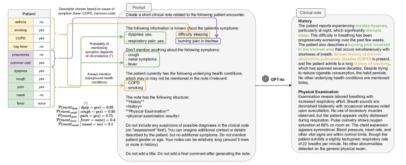
Figure 6: Additional example prompt with generated note. Since there are multiple causes for the symptom dyspnea (smoking, COPD) which are present in the patient, the descriptor “difficulty sleeping” was chosen randomly out of the bag of descriptors for smoking and COPD from table 5. For respiratory pain, the descriptor “burning pain in the trachea” was chosen randomly out of the descriptors for common cold. While cough and COPD are also possible causes for respiratory pain, and are present in the patient, common cold overrules the two according to our strategy outlined in Section 2.2.

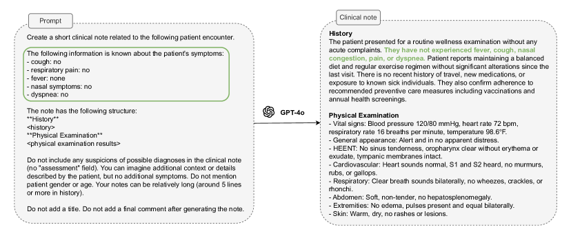
Figure 7: Example of what would happen if we simply extended the general prompt to the 3629 cases where the patient does not experience any respiratory symptoms. There would be little variation in these notes, as these patients seem to visit the doctor’s office for no reason. It is more realistic to encourage the LLM to generate a note which describes a patient visiting for a non-respiratory complaint, like the prompts shown in Figures 4 and 8.

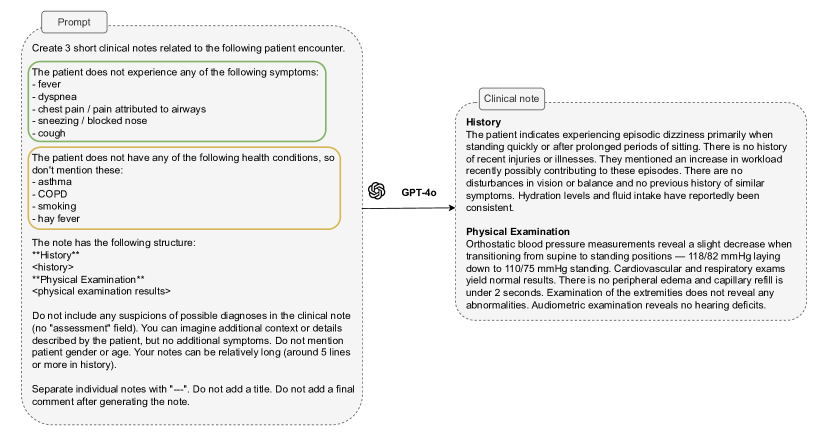
Figure 8: Prompt used for cases where patient does not experience any respiratory symptoms or have any underlying respiratory health condition. We show one of the three generated notes.

Appendix B Symptom predictor baselines

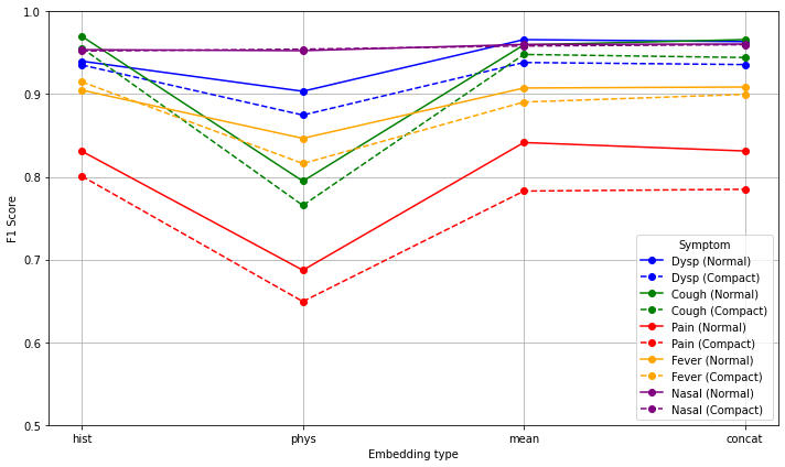
Figure 9: Results for the neural-text baseline for the different embedding types. We show F1-scores over the test set for both the normal and compact versions of the notes. Figure best viewed in colour.

B.1 BN-tab

We learn a Bayesian network over the training data, providing the structure over all variables as in Figure 2. For the variables asthma, smoking, hay fever, COPD, season, pneumonia, common cold, fever and self-employed, we learn the conditional probability tables (CPTs) from the training data using maximum likelihood estimation (which comes down to counting co-occurrences of child and parent values for each entry in the CPT). We use the pgmpy library (Ankur Ankan and Abinash Panda, 2015) with a K2 prior as a smoothing strategy to initialize empty CPTs.

As support for learning Noisy-OR distributions is not provided in pgmpy, we learn these parameters with a custom training loop. We formulate the likelihood as in Equation (2), and learn the parameters $p_{i}$ in Equations (3) through (6) for the variables dyspnea, cough, pain and nasal through maximum likelihood estimation by iterating over the train set for 10 epochs, using an Adam optimizer with a batch size of 50, a learning rate of 0.01 and random initialization of each parameter. To integrate the learned Noisy-OR distributions in the Bayesian network, we turn them into fully specified CPTs. To obtain these, we simply evaluate Equation (2) for all possible combinations of child and parent values. While this results in large and inefficient CPTs, the automated inference engine bulit into pgmpy library does not support Noisy-OR distributions directly. Note that both versions of the conditional distribution are equivalent, so we do not incur a loss in precision.

Similarly, the coefficients in the logistic regression model for antibiotics and the Poisson regression model for #days are learned using maximum likelihood estimation over the training set. The likelihood is expressed as in Equation (7) and Equations (8) and (9) respectively, with learnable parameters in place of each coefficient. We iterate over the train set for 15 epochs, again using an Adam optimizer with a batch size of 50, a learning rate of 0.01 and random initialization of each parameter. Finally, we turn the logistic regression and Poisson regression models into CPTs by evaluating Equations (7), (8) and (9) for all combinations of parent and child values. For the variable #days, we needed to turn each discrete number of days into a category, because pgmpy only provides automated inference for Bayesian networks consisting of exclusively categorical variables. This results in a large CPT containing one row per possible number of days, which range from 0 to 15 in our training dataset, and one column for each combination of the 7 parent variables. To allow for a possible larger maximum number of days in the test set, we create a category $\geq\text{{15 days}}$, which is defined as one minus the summed probability of all other days.

Once we have learned all parameters in the joint distribution, we can evaluate the Bayesian network’s ability to predict each of the symptoms. For each evidence setting (as defined in the main text), we apply variable elimination with each of the symptoms as a target variable. Looking at the causal structure in Figure 2, we note that the model never has to marginalize over the many rows in the learned #days CPT, since it is never a target variable. This makes automated inference feasible in our case.

B.2 XGBoost-tab

We use the xgboost library in combination with sklearn. We train separate classifiers per symptom, one for each setting, which means we train 15 classifiers total. We tune the hyperparameters separately for each classifier, using 5-fold cross validation with F1 as a scoring metric (macro-F1 for fever).

The classifiers for the symptoms dysp, cough, pain and nasal use a binary logistic objective and logloss as an evaluation metric within the XGBoost training procedure, while the classifiers for the symptom fever use the multi-softmax objective with multiclass logloss as an evaluation metric. The scale_pos_weight parameter is set to the ratio of negative over positive samples for the binary classifiers. For the fever classifier, we address class imbalance by setting class_weight = balanced, which ensures that samples from less frequent classes (in our case low and high fever) receive higher weight in the loss calculation. We use grid search to find the best hyperparameter configuration, where the following sets of options are explored:

• n_estimators: $\{50,100,200\}$

• max_depth: $\{2,3,4,5\}$

• learning_rate: $\{0.01,0.1,0.2\}$

• subsample: $\{0.8,1\}$

• colsample_bytree: $\{0.8,1\}$

• gamma: $\{0,0.1,0.3\}$

• min_child_weight: $\{1,5,10\}$

B.3 Neural-text

The pretrained BioLORD encoder (Remy, Demuynck, and Demeester, 2024) was obtained through the huggingface library. The encoder outputs 768-dimensional sentence embeddings. Since the full text did not fit into the context window, we embedded each sentence separately, and then combined them using our strategies outlined in the main text. To split the text into sentences, we used the nltk package. The settings hist, phys and mean all result in a text embedding of 768 dimensions, while the setting concat results in a text embedding of 2*768 dimensions.

These embeddings are fed into a linear layer with 256 neurons, which is then transformed into a single output neuron, followed by a Sigmoid activation. For the classifiers that predict fever, three output neurons followed by a Softmax activation are used instead, one for each class. While the embeddings remain fixed, we learn the parameters in the hidden and output layers using cross-entropy as a loss function over the training set. We train a separate classifier for each symptom, setting and difficulty of the text (normal vs. compact). For the binary symptoms, we train for $15$ epochs using the Adam optimizer with a batch size of $100$, a learning rate of $0.001$ and weight_decay set to $1\mathrm{e}-5$. The classifier for $fever$ tended to collapse more easily, which is why we train it for $30$ epochs with a lower learning rate of $5\mathrm{e}-4$ instead. These hyperparameters were obtained using a mix of manual tuning and grid search with 5-fold cross validation over the training set.

Results for the different embedding types, which are reported numerically in Table 7, are shown in Figure 9.

B.4 Neural-text-tab

For each evidence setting, we select the relevant set of tabular features and transform them into a numerical representation. We use a one-hot encoding for the categorical (binary or multiclass) features, and normalize the #days feature using the StandardScaler from sklearn. This tabular feature representation is then concatenated with the text representation we obtained in the previous baseline. Both are fed into the same architecture described in Section B.4, adapting the dimension of the input layer accordingly. For example, for the dyspnea classifier in the evidence setting all, the input dimension becomes $768+17$. We use the same hyperparameters as in the neural-text baseline to ensure a fair comparison. All other training details remain the same.

References

- Ankur Ankan and Abinash Panda (2015) Ankur Ankan; and Abinash Panda. 2015. pgmpy: Probabilistic Graphical Models using Python. In Proceedings of the 14th Python in Science Conference, 6 – 11.
- Ceritli et al. (2023) Ceritli, T.; Ghosheh, G. O.; Chauhan, V. K.; Zhu, T.; Creagh, A. P.; and Clifton, D. A. 2023. Synthesizing mixed-type electronic health records using diffusion models. arXiv preprint arXiv:2302.14679.
- Ford et al. (2016) Ford, E.; Carroll, J. A.; Smith, H. E.; Scott, D.; and Cassell, J. A. 2016. Extracting information from the text of electronic medical records to improve case detection: a systematic review. J Am Med Inform Assoc, 23(5): 1007–1015.
- Guan et al. (2019) Guan, J.; Li, R.; Yu, S.; and Zhang, X. 2019. A method for generating synthetic electronic medical record text. IEEE/ACM transactions on computational biology and bioinformatics, 18(1): 173–182.
- Hahn and Oleynik (2020) Hahn, U.; and Oleynik, M. 2020. Medical information extraction in the age of deep learning. Yearbook of medical informatics, 29(01): 208–220.
- Hernandez et al. (2022) Hernandez, M.; Epelde, G.; Alberdi, A.; Cilla, R.; and Rankin, D. 2022. Synthetic data generation for tabular health records: A systematic review. Neurocomputing, 493: 28–45.
- Huang, Altosaar, and Ranganath (2019) Huang, K.; Altosaar, J.; and Ranganath, R. 2019. Clinicalbert: Modeling clinical notes and predicting hospital readmission. arXiv preprint arXiv:1904.05342.
- Koller and Friedman (2009) Koller, D.; and Friedman, N. 2009. Probabilistic Graphical Models: Principles and Techniques. Adaptive computation and machine learning. MIT Press. ISBN 9780262013192.
- Kwon et al. (2024) Kwon, Y.; Kim, J.; Lee, G.; Bae, S.; Kyung, D.; Cha, W.; Pollard, T.; Johnson, A.; and Choi, E. 2024. EHRCon: Dataset for Checking Consistency between Unstructured Notes and Structured Tables in Electronic Health Records. arXiv preprint arXiv:2406.16341.
- Labrak et al. (2024) Labrak, Y.; Bazoge, A.; Morin, E.; Gourraud, P.-A.; Rouvier, M.; and Dufour, R. 2024. Biomistral: A collection of open-source pretrained large language models for medical domains. arXiv preprint arXiv:2402.10373.
- Lee (2018) Lee, S. H. 2018. Natural language generation for electronic health records. NPJ digital medicine, 1(1): 63.
- Lehman and Johnson (2023) Lehman, E.; and Johnson, A. 2023. Clinical-t5: Large language models built using mimic clinical text. PhysioNet.
- Li et al. (2020) Li, Y.; Rao, S.; Solares, J. R. A.; Hassaine, A.; Ramakrishnan, R.; Canoy, D.; Zhu, Y.; Rahimi, K.; and Salimi-Khorshidi, G. 2020. BEHRT: transformer for electronic health records. Scientific reports, 10(1): 7155.
- Liu et al. (2022) Liu, S.; Wang, X.; Hou, Y.; Li, G.; Wang, H.; Xu, H.; Xiang, Y.; and Tang, B. 2022. Multimodal data matters: language model pre-training over structured and unstructured electronic health records. IEEE Journal of Biomedical and Health Informatics, 27(1): 504–514.
- Lundberg et al. (2020) Lundberg, S. M.; Erion, G.; Chen, H.; DeGrave, A.; Prutkin, J. M.; Nair, B.; Katz, R.; Himmelfarb, J.; Bansal, N.; and Lee, S.-I. 2020. From local explanations to global understanding with explainable AI for trees. Nature machine intelligence, 2(1): 56–67.
- Mujtaba et al. (2019) Mujtaba, G.; Shuib, L.; Idris, N.; Hoo, W. L.; Raj, R. G.; Khowaja, K.; Shaikh, K.; and Nweke, H. F. 2019. Clinical text classification research trends: Systematic literature review and open issues. Expert Syst Appl, 116: 494–520.
- OpenAI (2024) OpenAI. 2024. Models – GPT-4o. https://platform.openai.com/docs/models/gpt-4o. Online; accessed 12 August 2024.
- Peiffer-Smadja et al. (2020) Peiffer-Smadja, N.; Rawson, T.; Ahmad, R.; Buchard, A.; and et al. 2020. Machine learning for clinical decision support in infectious diseases: A narrative review of current applications. Clin Microbiol Infect, 26(5): 584–595.
- Quinn et al. (2022) Quinn, T. P.; Jacobs, S.; Senadeera, M.; Le, V.; and Coghlan, S. 2022. The three ghosts of medical AI: Can the black-box present deliver? Artificial intelligence in medicine, 124: 102158.
- Rabaey et al. (2024) Rabaey, P.; Deleu, J.; Heytens, S.; and Demeester, T. 2024. Clinical Reasoning over Tabular Data and Text with Bayesian Networks. In International Conference on Artificial Intelligence in Medicine, 229–250. Springer.
- Rasmy et al. (2021) Rasmy, L.; Xiang, Y.; Xie, Z.; Tao, C.; and Zhi, D. 2021. Med-BERT: pretrained contextualized embeddings on large-scale structured electronic health records for disease prediction. NPJ digital medicine, 4(1): 86.
- Remy, Demuynck, and Demeester (2024) Remy, F.; Demuynck, K.; and Demeester, T. 2024. BioLORD-2023: semantic textual representations fusing large language models and clinical knowledge graph insights. Journal of the American Medical Informatics Association, ocae029.
- Rudin (2019) Rudin, C. 2019. Stop explaining black box machine learning models for high stakes decisions and use interpretable models instead. Nature machine intelligence, 1(5): 206–215.
- Sanchez et al. (2022) Sanchez, P.; Voisey, J. P.; Xia, T.; Watson, H. I.; O’Neil, A. Q.; and Tsaftaris, S. A. 2022. Causal machine learning for healthcare and precision medicine. Royal Society Open Science, 9(8): 220638.
- Singhal et al. (2023) Singhal, K.; Azizi, S.; Tu, T.; Mahdavi, S. S.; Wei, J.; Chung, H. W.; Scales, N.; Tanwani, A.; Cole-Lewis, H.; Pfohl, S.; et al. 2023. Large language models encode clinical knowledge. Nature, 620(7972): 172–180.
- Tian et al. (2024) Tian, S.; Jin, Q.; Yeganova, L.; Lai, P.-T.; Zhu, Q.; Chen, X.; Yang, Y.; Chen, Q.; Kim, W.; Comeau, D. C.; et al. 2024. Opportunities and challenges for ChatGPT and large language models in biomedicine and health. Briefings in Bioinformatics, 25(1): bbad493.
- Veitch, Sridhar, and Blei (2020) Veitch, V.; Sridhar, D.; and Blei, D. 2020. Adapting text embeddings for causal inference. In Conference on Uncertainty in Artificial Intelligence, 919–928. PMLR.
- Wang et al. (2018) Wang, Y.; Wang, L.; Rastegar-Mojarad, M.; Moon, S.; Shen, F.; Afzal, N.; Liu, S.; Zeng, Y.; Mehrabi, S.; Sohn, S.; et al. 2018. Clinical information extraction applications: a literature review. Journal of biomedical informatics, 77: 34–49.
- Xu et al. (2019) Xu, K.; Lam, M.; Pang, J.; Gao, X.; Band, C.; Mathur, P.; Papay, F.; Khanna, A. K.; Cywinski, J. B.; Maheshwari, K.; et al. 2019. Multimodal machine learning for automated ICD coding. In Machine learning for healthcare conference, 197–215. PMLR.
- Zhang et al. (2020) Zhang, D.; Yin, C.; Zeng, J.; Yuan, X.; and Zhang, P. 2020. Combining structured and unstructured data for predictive models: A deep learning approach. BMC Med Inform Decis Mak, 20(1): 280.
- Zhao et al. (2024) Zhao, H.; Chen, H.; Yang, F.; Liu, N.; Deng, H.; Cai, H.; Wang, S.; Yin, D.; and Du, M. 2024. Explainability for large language models: A survey. ACM Transactions on Intelligent Systems and Technology, 15(2): 1–38.