Domain-wall Skyrmion phase of QCD in magnetic field: Gauge field dynamics

Abstract

The ground state of QCD in sufficiently strong magnetic field at finite baryon density is an inhomogeneous state consisting of an array of solitons, called the chiral soliton lattice (CSL). It is, however, replaced in a region with higher density and/or magnetic field by the so-called domain-wall Skyrmion(DWSk) phase where Skyrmions are created on top of the CSL. This was previously proposed within the Bogomol’nyi-Prasad-Sommerfield (BPS) approximation neglecting a gauge field dynamics and taking into account its effect by a flux quantization condition. In this paper, by taking into account dynamics of the gauge field, we show that the phase boundary between the CSL and DWSk phases beyond the BPS approximation is identical to the one obtained in the BPS approximation. We also find that domain-wall Skyrmions are electrically charged with the charge one as a result of the chiral anomaly.

1 Introduction

The phase diagram of Quantum Chromodynamics (QCD) receives a quite extensive attention, especially under extreme conditions like high baryon density, pronounced magnetic fields, and rapid rotation Fukushima:2010bq . In particular, strong magnetic fields have received quite intense attention because of their relevance in the interior of neutron stars and heavy-ion collisions. First principle calculation of QCD at finite density is difficult due to the sign problem. On the other hand, at low energy QCD can be described model independently by the chiral Lagrangian or the chiral perturbation theory (ChPT) Scherer:2012xha ; Bogner:2009bt ; when chiral symmetry undergoes spontaneous breaking, there appear massless Nambu-Goldstone (NG) bosons or pions, which are dominant at low energy. The low-energy dynamics of QCD is governed by these light modes in terms of the aforementioned ChPT centered on the pionic degree of freedom. Importantly, this description is model independently dictated by symmetries and only modulated by certain constants, including the pion’s decay constant $f_{\pi}$ and quark masses $m_{\pi}$. Effects of external magnetic fields $B$ and finite chemical potential $\mu_{\textrm{B}}$ can be incorporated in the ChPT; It is accompanied by the Wess-Zumino-Witten (WZW) term containing an anomalous coupling of the neutral pion $\pi^{0}$ to the magnetic field via the chiral anomaly Son:2004tq ; Son:2007ny in terms of the Goldstone-Wilczek current Goldstone:1981kk ; Witten:1983tw , determined to reproduce the so-called chiral separation effect Vilenkin:1980fu ; Son:2004tq ; Metlitski:2005pr ; Fukushima:2010bq ; Landsteiner:2016led in terms of the neutral pion $\pi^{0}$.

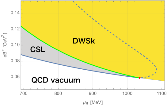
Figure 1: The phase diagram of QCD in the $\mu_{\rm B}$-$eB^{z}$ plane. The blue solid and grey curves are the boundary with QCD vacuum above which CSL or DWSk phases are ground states, respectively. The green curve is the phase boundary between the CSL and DWSk phases previously obtained in the BPS approximation, which we show in this paper is valid even taking into account gauge field dynamics. The CSL state remains metastable between the green and blue dotted curves, that becomes unstable beyond the blue dotted curve where the CPC occurs. The red point denotes a tricritical point where the DWSk and CSL phases and QCD vacuum meet.

In this set up, it was found in Refs. Son:2007ny ; Eto:2012qd ; Brauner:2016pko that under a sufficiently strong magnetic field $B$ satisfying $B\geq B_{\rm CSL}={16\pi m_{\pi}/f_{\pi}^{2}}{e\mu_{\textrm{B}}}$, the ground state of QCD with two flavors becomes inhomogeneous in the form of a chiral soliton lattice (CSL) consisting of a stack of domain walls or solitons carrying a baryon number (the blue solid and grey curves in Fig. 1). The quantum nucleation of such CSLs was studied in Refs. Eto:2022lhu ; Higaki:2022gnw , while the extension to include the $\eta^{\prime}$ meson leads to quasicrystals Qiu:2023guy . Although these results are based on zero temperature analyses, it was also shown that thermal fluctuations enhance their stability Brauner:2017uiu ; Brauner:2017mui ; Brauner:2021sci ; Brauner:2023ort . However, such a CSL state was found to exhibit two kinds of instabilities, with replaced by another state. One is a charged pion condensation (CPC) in a region of higher density and/or stronger magnetic field, asymptotically expressed at large $B$ as $B\geq B_{\rm CPC}\sim{16\pi^{4}f_{\pi}^{4}}/{\mu_{\rm B}^{2}}$ Brauner:2016pko above which the CSL becomes unstable, and was proposed to go to an Abrikosov’s vortex lattice or a baryon crystal Evans:2022hwr ; Evans:2023hms . Another instability of the CSL relevant to our study occurring below the CPC instability corresponds to the appearance of a domain-wall Skyrmion (DWSk) phase in a region $B\geq B_{\rm DWSk}(<B_{\rm CPC})$ (denoted by the green curve in Fig. 1) in which Skyrmions are created on top of the solitons in the ground state Eto:2023lyo ; Eto:2023wul . These two instability curves meet at a single tricritical point $(\mu_{\rm c},B_{\rm c})=\left({16\pi f_{\pi}^{2}}/{3m_{\pi}},{3m_{\pi}^{2}}/{e}\right)\approx\left(1.03\;\;{\rm GeV},0.06{\rm GeV}^{2}\sim 1.0\times 10^{19}{\rm G}\right)$ (denoted by the red dot in Fig. 1) on the critical curve $B=B_{\rm CSL}$ of the CSL phase. Skyrmions are topological solitons supported by the third homotopy group $\pi_{3}[{\rm SU}(N_{\rm F})]\simeq{\mathbb{Z}}$ in the chiral Lagrangian complemented by a four-derivative Skyrme term originally proposed to describe baryons Skyrme:1962vh where $N_{\rm F}$ is a number of flavors, and in our context the interplay between Skyrmion crystals at zero magnetic field and the CSL was studied in Refs. Kawaguchi:2018fpi ; Chen:2021vou ; Chen:2023jbq . The domain-wall Skyrmions are composite states of a domain wall and Skyrmions, initially introduced in the field theoretical models in 2+1 dimensions Nitta:2012xq ; Kobayashi:2013ju ; Jennings:2013aea and in 3+1 dimensions Nitta:2012wi ; Nitta:2012rq ; Gudnason:2014nba ; Gudnason:2014hsa ; Eto:2015uqa ; Nitta:2022ahj . In QCD, Skyrmions in the bulk are absorbed into a chiral soliton to become topological lumps (or baby Skyrmions) supported by $\pi_{2}(S^{2})\simeq{\mathbb{Z}}$ in an O(3) sigma model or the ${\mathbb{C}}P^{1}$ model, constructed by the moduli approximation Manton:1981mp ; Eto:2006uw ; Eto:2006pg as the effective worldvolume theory on a soliton Eto:2023lyo . One of the important features is that one lump in the soliton corresponds to two Skyrmions in the bulk, and thus they are bosons Amari:2024mip . Domain-wall Skyrmions in multiple chiral solitons (that is a CSL) are Skyrmion chains Eto:2023wul , giving a more precise phase boundary between the CSL and DWSk phases.

In the previous works Eto:2023lyo ; Eto:2023wul , the so-called Bogomol’nyi-Prasad-Sommerfield (BPS) approximation was employed: lump solutions in the domain-wall effective theory are approximated by BPS lumps with neglecting the gauge coupling, and subsequently taken into account the gauge field through a flux quantization condition. On the other hand, in our previous paper Amari:2024adu , we constructed full gauged lump solutions in a gauged ${\mathbb{C}}P^{1}$ model and found that the flux quantization is only $15\%$ satisfied, and their energy (mass) are about $10\%$ less that that of the BPS lump. We could expect a similar thing happens for domain-wall Skyrmions.

In this paper, we investigate the gauge field dynamics to construct gauged (anti-)lump solutions beyond the BPS approximation. First, we point out that anti-lumps in the domain-wall effective theory correspond to Skyrmions in the bulk, which can have negative energy due to the WZW term in the DWSk phase, while lumps in the wall correspond to anti-Skyrmions in the bulk which are always excited states. We then find a critical gauge coupling above which a regular solution of gauged anti-lump solutions exist stably and below which solutions become singular. On contrary, gauged lumps (anti-Skyrmions) are always regular and stable. Our main results are twofold. First, we find that gauged anti-lumps are singular in a realistic gauge coupling. Nevertheless, their energy is finite coinciding with the BPS energy, and becomes negative in the DWSk phase. This implies that the phase boundary between the DWSk and CSL phases is unchanged from the BPS approximation. On the other hand, in strong gauge coupling, a region of regular solution expands and the DWSk phase expands in the phase diagram. Second, we find that gauged anti-lumps are electrically charged due to the chiral anomaly and their charges are one.

This paper is organized as follows. In Sec. 2 we review the chiral Lagrangian and the CSL phase. In Sec. 3, the DWSk is constructed in terms of the domain-wall effective theory. In Sec. 4, the phase boundary between the DWSk and CSL phases and properties of domain-wall Skyrmions are investigated. Section 5 is devoted to a summary and discussion.

2 The chiral soliton lattice in QCD

In this section, we give a review on chiral Lagrangian and CSL in order to fix our notations.

2.1 Chiral Lagrangian

In this paper, we take the metric $\eta_{\mu\nu}=(+,-,-,-)$. The chiral Lagrangian with $N_{F}=2$ flavors is given by

$${\cal L}_{\rm ChPT}=-\frac{1}{4}F_{\mu\nu}F^{\mu\nu}+\frac{f_{\pi}^{2}}{4}{\rm tr}D_{\mu}\Sigma^{\dagger}D^{\mu}\Sigma+{\rm tr}\left(M\Sigma+\text{h.c.}\right)\,,$$ (2.1)

where pions are parameterized by

$$\Sigma=\exp\left(\frac{i\tau^{a}\varphi^{a}}{f_{\pi}}\right)=\frac{1}{f_{\pi}}\left(\sigma+i\tau^{a}\pi^{a}\right)\,,\quad\left(\sigma^{2}+\pi^{a}\pi^{a}=f_{\pi}^{2}\right)\,,$$ (2.2)

the covariant derivative is given by

$$D_{\mu}\Sigma=\partial_{\mu}\Sigma+ieA_{\mu}\left[Q,\Sigma\right]\,,\qquad Q=\frac{\tau^{3}}{2}+\frac{1}{6}{\bf 1}_{2}\,,$$ (2.3)

and $M$ is the pion mass matrix explicitly given below. The charged pions are identified by $\pi^{\pm}\equiv\pi^{1}\mp i\pi^{2}$, and the covariant derivative on them is $D_{\mu}\pi^{\pm}=\left(\partial_{\mu}\pm ieA_{\mu}\right)\pi^{\pm}$. The $U(1)_{\rm EM}$ electromagnetic gauge transformation is given by

$$\Sigma\to e^{iQ\alpha(x)}\Sigma e^{-iQ\alpha(x)}~{},\quad\pi^{\pm}\to e^{\pm i\alpha(x)}\pi^{\pm}\,,\quad A_{\mu}\to A_{\mu}-e^{-1}\partial_{\mu}\alpha(x)\,.$$ (2.4)

In addition to ${\cal L}_{\rm ChPT}$, the WZW term is needed to reproduce the chiral anomaly. For the two flavors, $N_{F}=2$, it is given by

$${\cal L}_{\rm WZW}=-A_{\mu}^{\rm B}j_{\rm B}^{\mu}+\frac{\epsilon^{\mu\nu\alpha\beta}}{16\pi^{2}}\left(\frac{1}{3}eA_{\mu}{\rm tr}\left(L_{\nu}L_{\alpha}L_{\beta}\right)-\frac{ie^{2}}{4}F_{\mu\nu}A_{\alpha}{\rm tr}\left[\tau^{3}\left(L_{\beta}+R_{\beta}\right)\right]\right)\,,$$ (2.5)

where $A_{\mu}^{\rm B}$ is a baryon gauge field, and $j_{\rm B}^{\mu}$ is the Goldstone-Wilczek baryon number current, given by

$$j_{\rm B}^{\mu}=-\frac{1}{24\pi^{2}}\epsilon^{\mu\nu\alpha\beta}\left\{{\rm tr}\left(L_{\nu}L_{\alpha}L_{\beta}\right)-\frac{3ie}{2}\partial_{\nu}\left[A_{\alpha}{\rm tr}\left[\tau^{3}\left(L_{\beta}+R_{\beta}\right)\right]\right]\right\}\,,$$ (2.6)

with

$$L_{\mu}=\Sigma\partial_{\mu}\Sigma^{\dagger}\,,\quad R_{\mu}=\partial_{\mu}\Sigma^{\dagger}\Sigma\,.$$ (2.7)

Our notation of the totally anti-symmetric tensor is $\epsilon^{0123}=-\epsilon_{0123}=1$. After short algebras, the $N_{F}=2$ WZW term can be expressed as Son:2007ny

$${\cal L}_{\rm WZW}=-A_{\mu}^{\rm B}j^{\mu}_{\rm B}-\frac{e}{2}A_{\mu}j^{\mu}_{\rm B}\,.$$ (2.8)

Note that the baryon number in our notation is given by

$$N_{\rm B}=\int d^{3}x\,(-j_{\rm B}^{0})\,.$$ (2.9)

Thus, the $N_{\rm F}=2$ chiral Lagrangian we will work on in this paper can be summarized as

$${\cal L}_{\rm ChPT+WZW}=\frac{f_{\pi}^{2}}{4}{\rm tr}D_{\mu}\Sigma^{\dagger}D^{\mu}\Sigma+{\rm tr}\left(M\Sigma+\text{h.c.}\right)-\left(A_{\mu}^{\rm B}+\frac{e}{2}A_{\mu}\right)j^{\mu}_{\rm B}\,.$$ (2.10)

The energy functional corresponding to this Lagrangian is for static configurations:

$${\cal M}=\frac{1}{4}F_{ij}^{2}+\frac{f_{\pi}^{2}}{4}{\rm tr}D_{i}\Sigma^{\dagger}D_{i}\Sigma-{\rm tr}\left(M\Sigma+\text{h.c.}\right)+\left(A_{\mu}^{\rm B}+\frac{e}{2}A_{\mu}\right)j^{\mu}_{\rm B}.$$ (2.11)

We turn on a uniform background magnetic field $B_{i}=\frac{1}{2}\epsilon_{ijk}F^{jk}$. For ease of notation, we set the magnetic field being parallel to the $z=x^{3}$ axis as

$$(F^{23},F^{31},F^{12})=(0,0,-B^{z})\quad\Leftrightarrow\quad(A_{0},A_{1},A_{2},A_{3})=\left(0,\frac{B^{z}}{2}x^{2},-\frac{B^{z}}{2}x^{1},0\right)\,.$$ (2.12)

In addition, we introduce a non-zero baryon chemical potential through the temporal component of the baryonic $U(1)$ gauge field with the chemical potential $\mu_{\rm B}$ as

$$A^{\rm B}_{\mu}=(\mu_{\rm B},0,0,0)\,,\quad\mu_{\rm B}\geq 0\,.$$ (2.13)

2.2 The chiral soliton lattice

The CSL appears as the ground state in the presence of the sufficiently large background magnetic field and the finite baryon chemical potential. In order to show CSL solutions, it is sufficient to set $\varphi^{1}=\varphi^{2}=0$, in which $\Sigma$ reduces to

$$\Sigma=\exp\left(\frac{i}{f_{\pi}}\tau^{3}\varphi^{3}\right)\,,\quad L_{\mu}=R_{\mu}=-\frac{i}{f_{\pi}}\tau^{3}\partial_{\mu}\varphi^{3}\,.$$ (2.14)

Then, the Goldstone-Wilczek current can be expressed as

$$j_{\rm B}^{\mu}=\frac{e\epsilon^{\mu\nu\alpha\beta}}{4f_{\pi}\pi^{2}}\partial_{\nu}\left(A_{\alpha}\partial_{\beta}\varphi^{3}\right)=\frac{e\epsilon^{\mu\nu\alpha\beta}}{4f_{\pi}\pi^{2}}\left(\partial_{\nu}A_{\alpha}\right)\partial_{\beta}\varphi^{3}\,.$$ (2.15)

Assuming that $\varphi^{3}$ depends on the $x^{3}$ coordinate only, we have

$$j_{\rm B}^{0}=\frac{e\epsilon^{0ijk}}{4f_{\pi}\pi^{2}}\left(\partial_{i}A_{j}\right)\partial_{k}\varphi^{3}=-\frac{e}{4\pi^{2}f_{\pi}}B^{z}\partial_{3}\varphi^{3}\,,$$ (2.16)

where we have used Eq. (2.13) and our notation is $\epsilon^{123}=-\epsilon_{123}=1$. Then the chiral Lagrangian reduces to

$${\cal L}_{{\rm ChPT}+{\rm WZW}}=\frac{f_{\pi}^{2}}{2}\partial_{\mu}\chi^{3}\partial^{\mu}\chi^{3}+f_{\pi}^{2}m_{\pi}^{2}\cos\chi^{3}+\frac{eB^{z}\mu_{\rm B}}{4\pi^{2}}\frac{\partial\chi^{3}}{\partial x^{3}}\,,$$ (2.17)

where we have expressed the pion mass

$$M=\frac{f_{\pi}^{2}m_{\pi}^{2}}{4}{\bf 1}_{2}\,,$$ (2.18)

and $\chi^{3}$ is a dimensionless field defined by

$$\varphi^{3}=f_{\pi}\chi^{3}\,,$$ (2.19)

The Lagrangian in Eq. (2.17) is known as a chiral sine-Gordon model.

The equation of motion (EOM) for the above reduced Lagrangian (2.17) reads

$$\partial_{\mu}\partial^{\mu}\chi^{3}+m_{\pi}^{2}\sin\chi^{3}=0\,.$$ (2.20)

This is simply sine-Gordon equation. An analytic solution for multiple solitons, called the CSL, is

$$\chi^{3}_{\rm CSL}(\zeta)=2\,{\rm am}\left(\frac{m_{\pi}\zeta}{\kappa},\kappa\right)+\pi\,,$$ (2.21)

where $\zeta$ is defined by $\zeta=\vec{k}\cdot\vec{x}$ with $\vec{k}$ being a unit vector that specifies the normal direction to the solitons. Here, $\kappa$ is a real number within $0\leq\kappa\leq 1$, called the elliptic modulus. The elliptic modulus is related to a period $\ell$ of the CSL as

$$\ell=\frac{2\kappa K(\kappa)}{m_{\pi}}\,,$$ (2.22)

where $K$ is the complete elliptic integral of the first kind. A single sine-Gordon soliton corresponds to the limit $\kappa\to 1$ in which the period becomes infinite $\ell\to\infty$.

The tension of the single soliton (one period of CSL) is given by

$$\sigma_{\rm CSL}=4m_{\pi}f_{\pi}^{2}\left[\frac{2E(\kappa)}{\kappa}+\left(\kappa-\frac{1}{\kappa}\right)K(\kappa)\right]-\frac{ek^{3}B^{z}\mu_{\rm B}}{2\pi}\,.$$ (2.23)

The second term is minimized by $k^{3}=1$ and the solitons are perpendicular to the $x^{3}$ axis (the direction of the magnetic field). In what follows, we fix $\vec{k}=(0,0,1)$. To determine optimized $\kappa$ for given $B^{z}$ and $\mu_{\rm B}$, we minimize the mean tension $\sigma_{\rm CSL}/\ell$. The condition is

$$\frac{d}{d\kappa}\frac{\sigma_{\rm CSL}}{\ell}=\frac{m_{\pi}E(\kappa)\left(16\pi f_{\pi}^{2}mE(\kappa)-eB^{z}\kappa\mu_{\rm B}\right)}{4\kappa^{3}\left(\kappa^{2}-1\right)\pi K(\kappa)^{2}}=0\,.$$ (2.24)

This is satisfied by

$$\frac{E(\kappa)}{\kappa}=\frac{eB^{z}\mu_{\rm B}}{16\pi f_{\pi}^{2}m_{\pi}}\,.$$ (2.25)

Thus, the minimum tension of a single soliton is

$$\sigma_{\rm CSL}(\kappa)=4m_{\pi}f_{\pi}^{2}\left(\kappa-\frac{1}{\kappa}\right)K(\kappa)\,.$$ (2.26)

This is always negative so that CSL is energetically more favourable than the homogeneous QCD vacuum for any $\kappa$ in $0\leq\kappa\leq 1$. Note that the elliptic integral satisfies $E(\kappa)/\kappa\geq 1$. Combining this with Eq. (2.25), we find the condition that CSL is the ground state

$$\mu_{\rm B}\geq\frac{16\pi m_{\pi}f_{\pi}^{2}}{eB^{z}}\equiv\mu_{\rm B}^{(1)}\,.$$ (2.27)

The bound is saturated for the single soliton at $\kappa\to 1$, denoted the blue solid curves in Figs. 2 and 1.

Note that the CSL solution given in Eq. (2.21) corresponds to a contractible loop in the $SU(2)$ manifold, and thus it is unstable against local fluctuations in the absence of the background magnetic field. The local stability problem (condensation of the charged pions) was found to be equal to the Landau level problem, and the bound for the background magnetic field is given by Son:2007ny ; Brauner:2016pko

$$eB^{z}\geq\frac{m_{\pi}^{2}}{\kappa^{2}}\left(2-\kappa^{2}+2\sqrt{1-\kappa^{2}+\kappa^{4}}\right)\equiv eB^{z(2)}\,.$$ (2.28)

The threshold value of $\mu_{\rm B}$ corresponding to $B^{z(2)}$ is implicitly given by $\kappa$ through Eq. (2.25), denoted by the blue dotted curve in Figs. 2 and 1, the phase diagram in the $\mu_{\rm B}$-$eB^{z}$ plane.

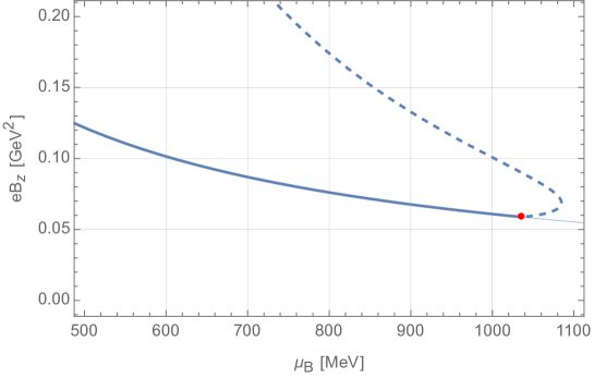
Figure 2: The homogeneous QCD vacuum is below the solid curve corresponding to the single CS limit ($\kappa\to 1$) with $\mu_{\rm B}=\mu_{\rm B}^{(1)}$ given in Eq. (2.27). The dashed curve corresponds to $B^{z}=B^{z(2)}$ given in Eq. (2.28). The CSL is (meta)stable between the solid and dashed curves. The red point is located at $\left(\dfrac{16\pi f_{\pi}^{2}}{3m_{\pi}},3m_{\pi}^{2}\right)$. We use $m_{\pi}=140$ MeV and $f_{\pi}=93$ MeV for an illustration.

3 The effective theory of non-Abelian chiral solitons

In the previous section, we have reviewed the CSL, an infinite array of the flat solitons perpendicular to the $x^{3}$ axis. Both global and local stabilities were clarified, but there is a loophole corresponding to possibility that a topologically nontrivial excitation arises on the flat solitons. Usually, a topological excitation costs some energy compared to a homogeneous vacuum (corresponding to the flat solitons in our case), so one might think such topologically nontrivial states do not change stability of CSL. However, it is not the case, because the WZW term in the presence of nonzero background magnetic field contributes the energy negatively.

3.1 Non-Abelian chiral soliton lattice

In order to include topologically nontrivial excitation on CSL, we first construct a low energy effective theory on CSL by using a standard moduli approximation method.

If we turn off the electromagnetic charge of the pions, the vector-like $SU(2)$ acting on

$$\Sigma\to g\Sigma g^{\dagger}\,,\quad g\in SU(2)\,$$ (3.1)

is genuine symmetry of the model. Then we can produce new CSL solutions by taking

$$\Sigma_{0}=\exp\left(i\tau^{3}\chi_{\rm CSL}^{3}\right)\,.$$ (3.2)

The solution can be parameterized by two component complex vector $\phi$ as follows

$$\Sigma=g\Sigma_{0}g^{\dagger}=\exp\left(ig\tau^{3}g^{\dagger}\chi_{\rm CSL}^{3}\right)=\exp\left(2i\phi\phi^{\dagger}\chi_{\rm CSL}^{3}\right)u^{-1}\,,$$ (3.3)

where $u$ is defined by $u=e^{i\chi_{\rm CSL}^{3}}$, and $\phi^{T}=(\phi_{1},\phi_{2})$ is given by $g$ as

$$g\tau_{3}g^{{\dagger}}=2\phi\phi^{{\dagger}}-\bm{1}_{2}\,.$$ (3.4)

Note that $\phi$ satisfies $\phi^{{\dagger}}\phi=1$, and its phase is ambiguous. Thus the new solutions are one to one correspondence to $S^{3}/S^{1}\simeq\mathbb{C}P^{1}$. By using the following identity

$$\exp\left(2i\phi\phi^{\dagger}\chi^{3}_{\rm CSL}\right)={\bf 1}+(u^{2}-1)\phi\phi^{\dagger}\,,$$ (3.5)

$\Sigma$ can be reexpressed as

$$\Sigma=\left[{\bf 1}+(u^{2}-1)\phi\phi^{\dagger}\right]u^{-1}\,.$$ (3.6)

Of course, $\phi$ is the genuine moduli parameter only when $B^{z}=0$. It is only approximately moduli parameter for $B^{z}\neq 0$.

Let us promote the moduli parameter $\phi$ of the CSL to an effective field on the worldvolume of CSL as $\phi=\phi(x^{\alpha})$ ($\alpha=0,1,2$), and derive a low energy effective action. The gauge field is assumed to depend on only $x^{\alpha}$ as

$$A_{0,3}=a_{0,3}(x^{\alpha})\,,\quad A_{1,2}={\cal A}_{1,2}(x^{1},x^{2})+a_{1,2}(x^{\alpha})\,,$$ (3.7)

where ${\cal A}_{1,2}$ is the background configuration

$${\cal A}_{a}=\frac{B^{z}}{2}\epsilon_{ab}x^{b}\,,\quad(a,b=1,2)\,.$$ (3.8)

In the following, we shall take the axial gauge

$$A_{3}=a_{3}=0\,.$$ (3.9)

3.2 The effective theory of the soliton worldvolume

Here, we construct the effective worldvolume theory on the solitons by the moduli approximation, sometimes called the Manton approximation Manton:1981mp ; Eto:2006pg ; Eto:2006uw . In this method, we promote the moduli parameters of the solitons to fields on the worldvolume $(x^{0},x^{1},x^{2})$, and integrate out the codimension $x^{3}$.

3.2.1 The chiral Lagrangian part

The covariant derivatives of $\Sigma$ read

$$D_{3}\Sigma = ge^{i\tau^{3}\chi_{\rm CSL}^{3}}i\tau^{3}\partial_{3}\chi_{\rm CSL}^{3}g^{\dagger}\,,$$ (3.10)

$$D_{\alpha}\Sigma = (u-u^{-1})\left((D^{\alpha}\phi)\phi^{\dagger}+\phi D^{\alpha}\phi^{\dagger}\right)\,,$$ (3.11)

with

$$D_{\alpha}\phi=\partial_{\alpha}\phi+i\frac{e}{2}A_{\alpha}\tau^{3}\phi\,,\quad D_{\alpha}\phi^{\dagger}=\partial_{\alpha}\phi^{\dagger}-i\frac{e}{2}\phi^{\dagger}\tau^{3}A_{\alpha}\,,$$ (3.12)

and the electromagnetic $U(1)_{\rm EM}$ gauge transformation is

$$\phi\to e^{i\frac{\tau^{3}}{2}\alpha(x)}\phi\,.$$ (3.13)

It is straightforward to obtain the following

$${\rm tr}D_{3}\Sigma^{\dagger}D^{3}\Sigma = 2\partial_{3}\chi_{\rm CSL}^{3}\partial^{3}\chi_{\rm CSL}^{3}\,,$$ (3.14)

$${\rm tr}D_{\alpha}\Sigma^{\dagger}\partial^{\alpha}\Sigma = -2(u-u^{-1})^{2}\left[D_{\alpha}\phi^{\dagger}D^{\alpha}\phi+(\phi^{\dagger}D_{\alpha}\phi)(\phi^{\dagger}D^{\alpha}\phi)\right]\,.$$ (3.15)

Plugging these into the chiral Lagrangian (2.1), and integrating it over $x^{3}$ for one period $\ell$, we find

$${\cal L}_{\rm ChPT}^{\rm eff} = \int^{\ell}_{0}dx^{3}\,\left\{\frac{f_{\pi}^{2}}{4}{\rm tr}D_{\mu}\Sigma^{\dagger}D^{\mu}\Sigma+{\rm tr}\left(M\Sigma+\text{h.c.}\right)\right\}$$ (3.16)

$$= -4m_{\pi}f_{\pi}^{2}\left[\frac{2E(\kappa)}{\kappa}+\left(\kappa-\frac{1}{\kappa}\right)K(\kappa)\right]$$

$$+~{}{\cal C}(\kappa)\left[D_{\alpha}\phi^{\dagger}D^{\alpha}\phi+(\phi^{\dagger}D_{\alpha}\phi)(\phi^{\dagger}D^{\alpha}\phi)\right]\,,$$

where we have defined the Kähler class

$${\cal C}(\kappa)\equiv-\frac{f_{\pi}^{2}}{2}\int^{\ell}_{0}dx^{3}\,(u-u^{-1})^{2}=\frac{16f_{\pi}^{2}}{3m_{\pi}}\beta(\kappa)\,,$$ (3.17)

with

$$\beta(\kappa)\equiv\frac{(2-\kappa^{2})E(\kappa)-2(1-\kappa^{2})K(\kappa)}{\kappa^{3}}\,.$$ (3.18)

Note that the first term in the final expression of Eq. (3.16) is constant and it can be rewritten by the tension of background CSL given in Eq. (2.26) as $4m_{\pi}f_{\pi}^{2}\left[\frac{2E(\kappa)}{\kappa}+\left(\kappa-\frac{1}{\kappa}\right)K(\kappa)\right]=\sigma_{\rm CSL}(\kappa)+\frac{eB^{z}\mu_{\rm B}}{2\pi}$. Thus, the chiral Lagrangian gives

$${\cal L}_{\rm ChPT}^{\rm eff}=-\sigma_{\rm CSL}(\kappa)-\frac{eB^{z}\mu_{\rm B}}{2\pi}+{\cal C}(\kappa)\left[D_{\alpha}\phi^{\dagger}D^{\alpha}\phi+(\phi^{\dagger}D_{\alpha}\phi)(\phi^{\dagger}D^{\alpha}\phi)\right]\,.$$ (3.19)

This is a $U(1)$ gauged ${\mathbb{C}}P^{1}$ model.

3.2.2 The WZW term

Let us next compute a contribution from the WZW term in Eq. (2.8). We first calculate the first term of Eq. (2.8). Since $A_{0}^{\rm B}=\mu_{\rm B}$ is the only nonzero component of $A_{\mu}^{\rm B}$, we only need $j_{\rm B}^{0}$. Let us decompose $j^{0}_{\rm B}$ given in Eq. (2.6) into two parts as

$$j_{\rm B}^{0}=-{\cal B}+\tilde{\cal B}\,,$$ (3.20)

with

$${\cal B} \equiv \frac{1}{24\pi^{2}}\epsilon^{ijk}{\rm tr}\left(L_{i}L_{j}L_{k}\right)\,,$$ (3.21)

$$\tilde{\cal B} \equiv \frac{ie}{16\pi^{2}}\epsilon^{ijk}\partial_{i}\left(A_{j}{\rm tr}\left[\tau^{3}\left(L_{k}+R_{k}\right)\right]\right)\,,$$ (3.22)

where we have used $\epsilon^{0ijk}=\epsilon^{ijk}$. Here $\tilde{\cal B}$ is the baryon number density for chiral solitons, while ${\cal B}$ is the baryon number density for Skyrmions whose spatial integration corresponds to the Skyrmion baryon number

$$N_{\rm B}^{\rm Sk}=\int d^{3}x\,{\cal B}\,.$$ (3.23)

We then express $j^{0}_{\rm B}$ in terms of the moduli field $\phi$. To this end, let us introduce a two by two projection matrix

$$P=\phi\phi^{\dagger}\,,\quad P^{\dagger}=P\,,\quad P^{2}=P\,.$$ (3.24)

Then, $\Sigma$ in Eq. (3.6) can be expressed as

$$\Sigma={\bf 1}u^{-1}+(u-u^{-1})P\,.$$ (3.25)

Using $u=e^{i\chi_{\rm CSL}^{3}}$, $\partial_{i}u=i\partial_{i}\chi_{\rm CSL}^{3}u$, and $\partial_{i}u^{-1}=-i\partial_{i}\chi_{\rm CSL}^{3}u^{-1}$, we can show

$$L_{i}=i\partial_{i}\chi_{\rm CSL}^{3}({\bf 1}-2P)-(1-u^{-2})\partial_{i}P-(u-u^{-1})^{2}P\partial_{i}P\,,$$ (3.26)

for $i=1,2,3$. Similarly, we have

$$R_{i}=i\partial_{i}\chi_{\rm CSL}^{3}({\bf 1}-2P)-(1-u^{-2})\partial_{i}P-(u-u^{-1})^{2}\partial_{i}PP\,.$$ (3.27)

Plugging these into Eq. (3.21), we obtain

$${\cal B}=\frac{1}{8\pi^{2}}{\rm tr}[L_{1},L_{2}]L_{3}=\frac{(u-u^{-1})^{2}\partial_{3}\chi_{\rm CSL}^{3}}{2\pi}\times q\,,$$ (3.28)

where we have defined

$$q\equiv-\frac{i}{2\pi}{\rm tr}\left[\partial_{1}P,\partial_{2}P\right]P=-\frac{i}{2\pi}\epsilon^{ab}\partial_{a}\phi^{\dagger}\partial_{b}\phi\,,$$ (3.29)

which is the topological lump number density associated with $\pi_{2}(\mathbb{C}P^{1})\simeq{\mathbb{Z}}$, such that

$$N_{\rm lump}\equiv\int d^{2}x\,q\in\mathbb{Z}\,.$$ (3.30)

For the CSL solution, we have

$$\int_{0}^{\ell}dx^{3}\,(u-u^{-1})^{2}\partial_{3}\chi^{3}_{\rm CSL}=-4\pi\,.$$ (3.31)

Therefore, we have

$$\int^{\ell}_{0}dx^{3}\,{\cal B}=-2q\,.$$ (3.32)

By integrating this over $x^{1}$ and $x^{2}$, we find a relation between the baryon and lump numbers as

$$N_{\rm B}^{\rm Sk}=\int d^{3}x\,{\cal B}=-2N_{\rm lump}\in 2\mathbb{Z}\,.$$ (3.33)

Next we compute $\tilde{\cal B}$. To this end, we introduce $M_{k}$ by

$$M_{k}\equiv{\rm tr}\left[\tau^{3}\left(L_{k}+R_{k}\right)\right]=\left\{\begin{array}[]{ccl}-(u^{2}-u^{-2}){\rm tr}\left(\tau^{3}\partial_{k}P\right)&&k=1,2\\ -4i\partial_{3}\chi^{3}\,{\rm tr}(\tau^{3}P)&&k=3\end{array}\right.\,,$$ (3.34)

then $\tilde{\cal B}$ in Eq. (3.22) can be expressed as

$$\tilde{\cal B}=\frac{ie}{16\pi^{2}}\left[F_{12}M_{3}-(\partial_{2}M_{3}-\partial_{3}M_{2})A_{1}-(\partial_{3}M_{1}-\partial_{1}M_{3})A_{2}\right]\,.$$ (3.35)

The right hand side can explicitly be written in terms of $\phi$ as

$$\partial_{2}M_{3}-\partial_{3}M_{2} = -4i{\rm tr}\left[\tau^{3}\partial_{2}P\right]\partial_{3}\chi^{3}_{\rm CSL}+{\rm tr}\left[\tau^{3}\partial_{2}P\right]\partial_{3}\left(u^{2}-u^{-2}\right)\,,$$ (3.36)

$$\partial_{3}M_{1}-\partial_{1}M_{3} = 4i{\rm tr}\left[\tau^{3}\partial_{1}P\right]\partial_{3}\chi^{3}_{\rm CSL}-{\rm tr}\left[\tau^{3}\partial_{1}P\right]\partial_{3}\left(u^{2}-u^{-2}\right)\,.$$ (3.37)

Integrating these over a one period $\ell$ of CSL, we have

$$\int_{0}^{\ell}dx^{3}\,F_{12}M_{3} = -8\pi iF_{12}\,{\rm tr}\left(\tau^{3}P\right)\,,$$ (3.38)

$$\int_{0}^{\ell}dx^{3}\,\left(\partial_{2}M_{3}-\partial_{3}M_{2}\right)A_{1} = -8\pi i\,{\rm tr}\left[\tau^{3}\partial_{2}P\right]A_{1}\,,$$ (3.39)

$$\int_{0}^{\ell}dx^{3}\,\left(\partial_{3}M_{1}-\partial_{1}M_{3}\right)A_{2} = 8\pi i\,{\rm tr}\left[\tau^{3}\partial_{1}P\right]A_{2}\,,$$ (3.40)

where we have used $\int^{\ell}_{0}dx^{3}\,\partial_{3}\chi^{3}=2\pi$, $\int^{\ell}_{0}dx^{3}\,\partial_{3}(u^{2}-u^{-2})=0$, $A_{3}=0$, and the fact that $A_{1,2}$ does not depend on $x^{3}$. We thus find

$$\int^{\ell}_{0}dx^{3}\,\tilde{\cal B}=\frac{e}{2\pi}\left(F_{12}-A_{1}\partial_{2}+A_{2}\partial_{1}\right){\rm tr}\left[\tau^{3}P\right]=\frac{e}{2\pi}\epsilon^{ab}\partial_{a}\left(A_{b}{\rm tr}\left[\tau^{3}P\right]\right)\,.$$ (3.41)

Combining Eqs. (3.32) and (3.41), a contribution from the first term of the WZW term to the effective Lagrangian reads

$$\int^{\ell}_{0}dx^{3}\,\left(-A_{\mu}^{\rm B}j_{\rm B}^{\mu}\right) = -\mu_{\rm B}\int^{\ell}_{0}dx^{3}\,\left(-{\cal B}+\tilde{\cal B}\right)$$ (3.42)

$$= -\mu_{\rm B}\left\{2q+\frac{e}{2\pi}\epsilon^{ab}\partial_{a}\left(A_{b}{\rm tr}\left[\tau^{3}P\right]\right)\right\}\,.$$

There is another contribution from the second term of Eq. (2.8). The contribution from $A_{0}$ is the same as that of $A_{0}^{\rm B}$, so we immediately find

$$\int^{\ell}_{0}dx^{3}\,\left(-\frac{e}{2}A_{0}j_{\rm B}^{0}\right)=-\frac{e}{2}A_{0}\left\{2q+\frac{e}{2\pi}\epsilon^{ab}\partial_{a}\left(A_{b}{\rm tr}\left[\tau^{3}P\right]\right)\right\}.$$ (3.43)

There is no contribution of $A_{3}$ since we set $A_{3}=0$. For a contribution of $A_{a}$ $(a=1,2)$, one needs to compute $j_{\rm B}^{a}$ but it turns out to be zero as

$$j_{\rm B}^{a}=-\frac{1}{24\pi^{2}}\epsilon^{a\nu\alpha\beta}\left\{{\rm tr}\left(L_{\nu}L_{\alpha}L_{\beta}\right)-\frac{3ie}{2}\partial_{\nu}\left[A_{\alpha}{\rm tr}\left[\tau^{3}\left(L_{\beta}+R_{\beta}\right)\right]\right]\right\}=0\,,$$ (3.44)

because of $A_{3}=0$ and $\partial_{3}=0$. Eq. (3.43) implies that an electric charge is induced around a lump, mostly proportional to its lump charge density. This gives a source term in the Maxwell equation, and it is electrically charged. The first term in Eq. (3.43) is proportional to the lump charge density while the second term is to the soliton charge. In the case of a Skyrmion, the second term is a total derivative (for constant $A_{0}$) and does not contribute to the total electric charge. Then, one finds that a contribution to the electric charge of (anti-)Skyrmion is

$$Q_{e}^{\rm Sk}=\frac{1}{2}N_{\rm B}^{\rm Sk}=-N_{\rm lump}.$$ (3.45)

Finally, we gather ${\cal L}_{\rm ChPT}^{\rm eff}$ given in Eq. (3.19) and the contributions from the WZW term given in Eqs. (3.42) and (3.43) to obtain the low energy effective Lagrangian on the CSL background as

$${\cal L}^{\rm eff} = -\sigma_{\rm CSL}(\kappa)-\frac{eB^{z}\mu_{\rm B}}{2\pi}-\frac{\ell}{4}F_{\alpha\beta}F^{\alpha\beta}+{\cal C}(\kappa)\left[D_{\alpha}\phi^{\dagger}D^{\alpha}\phi+(\phi^{\dagger}D_{\alpha}\phi)(\phi^{\dagger}D^{\alpha}\phi)\right]$$ (3.46)

$$- \left(\mu_{\rm B}+\frac{e}{2}A_{0}\right)\left\{2q+\frac{e}{2\pi}\epsilon^{ab}\partial_{a}\left(A_{b}{\rm tr}\left[\tau^{3}P\right]\right)\right\}\,.$$

Here, we have included the gauge kinetic term as the third term, which is not localized on the soliton and is proportional to the period $\ell$.

3.2.3 Reformulation as $O(3)$ nonlinear sigma model

The ${\mathbb{C}}P^{1}$ model is equivalent to the $O(3)$ nonlinear sigma model because of ${\mathbb{C}}P^{1}\simeq S^{2}\simeq O(3)/O(2)$. Here we rewrite the above Lagrangian as the $O(3)$ model described by three component real scalar fields $\vec{n}$ defined by

$$\vec{n}=\phi^{\dagger}\vec{\tau}\phi\,,\quad\left[\vec{n}=\,{\rm tr}\left(\vec{\tau}P\right)\,,\quad P=\phi\phi^{\dagger}=\frac{1}{2}\left(I_{2}+\vec{n}\cdot\vec{\tau}\right)\right]\,.$$ (3.47)

This satisfies the constraint $\vec{n}^{2}=1$.

The electromagnetic $U(1)_{\rm EM}$ gauge transformation of $\vec{n}$ fields can be read from Eqs. (2.4) and (3.13) as

$$n_{1}+in_{2}\to e^{-i\alpha(x)}(n_{1}+in_{2})\,,\quad n_{3}\to n_{3}\,.$$ (3.48)

Note that $n_{1}+in_{2}$ is negatively charged under $U(1)_{\rm EM}$. Indeed, $n_{1}\pm in_{2}$ is essentially identified with the charged pion $\pi^{\mp}$ as

$$\pi^{\pm}=\frac{f_{\pi}}{2i}{\rm tr}\left[(\tau^{1}\mp i\tau^{2})\Sigma\right]=\frac{f_{\pi}(u-u^{-1})}{2i}\left(n_{1}\mp in_{2}\right)=f_{\pi}\left(n_{1}\mp in_{2}\right)\sin\chi^{3}_{\rm CSL}\,,$$ (3.49)

where we have used Eqs. (2.2) and (3.6).

Similarly, we have the following expression for the neutral components

$$\sigma=f_{\pi}\cos\chi^{3}_{\rm CSL}\,,\quad\pi^{0}=f_{\pi}n_{3}\sin\chi^{3}_{\rm CSL}\,.$$ (3.50)

Correspondingly, the covariant derivatives are translated as

$$D_{\alpha}\phi=\partial_{\alpha}\phi+i\frac{e}{2}A_{\alpha}\tau^{3}\phi\quad\Leftrightarrow\quad\left\{\begin{array}[]{l}D_{\alpha}(n_{1}+in_{2})=(\partial_{\alpha}-ieA_{\alpha})(n_{1}+in_{2})\\ D_{\alpha}n^{3}=\partial_{\alpha}n^{3}\end{array}\right.$$ (3.51)

Then one can easily show the following expression

$$D_{\alpha}\phi^{\dagger}D^{\alpha}\phi+(\phi^{\dagger}D_{\alpha}\phi)(\phi^{\dagger}D^{\alpha}\phi)=\frac{1}{4}D_{\alpha}\vec{n}\cdot D^{\alpha}\vec{n}\,.$$ (3.52)

Thus the effective Lagrangian with respect to $\vec{n}$ field is given by

$${\cal L}^{\rm eff} = -\sigma_{\rm CSL}-\frac{eB^{z}\mu_{\rm B}}{2\pi}-\frac{\ell}{4}F_{\alpha\beta}F^{\alpha\beta}+\frac{{\cal C}}{4}D_{\alpha}\vec{n}\cdot D^{\alpha}\vec{n}$$ (3.53)

$$- \left(\mu_{\rm B}+\frac{e}{2}A_{0}\right)\left\{2q+\frac{e}{2\pi}\epsilon^{ab}\partial_{a}\left(A_{b}n_{3}\right)\right\}\,,$$

where the lump charge $q$ given by Eq. (3.29) can be rewritten in terms of $\vec{n}$ as

$$q=\frac{1}{8\pi}\epsilon^{ij}\vec{n}\cdot(\partial_{i}\vec{n}\times\partial_{j}\vec{n})\,.$$ (3.54)

The last term in Eq. (3.53),

$$-\frac{e}{2}A_{0}\left\{2q+\frac{e}{2\pi}\epsilon^{ab}\partial_{a}\left(A_{b}n_{3}\right)\right\}\,,$$ (3.55)

implies that an electric charge is induced around a lump as mentioned above.

It is worth making a comment on similarity between the our effective theory and magnetic systems. If we force the $\vec{n}$ field to be constant and the gauge field is the uniform background $A_{a}={\cal A}_{a}$, the Hamiltonian reduces to the following form

$${\cal H}^{\rm eff}\to\left(\sigma_{\rm CSL}+\frac{\ell}{2}(B^{z})^{2}\right)+\frac{{\cal C}e^{2}(B^{z})^{2}}{16}(x^{2}+y^{2})(1-n_{3}^{2})+\frac{eB^{z}\mu_{\rm B}}{2\pi}\left(1-n_{3}\right)\,.$$ (3.56)

The second term is the contribution from the kinetic term $(D\vec{n})^{2}$, and the third term originates from the WZW term [the second line of Eq. (3.53)]. The former resembles the easy-axis potential that favors $n_{3}=\pm 1$. The latter is the same as the Zeeman-type potential that favors $n_{3}=+1$. Thus, our effective Lagrangian is similar to a ferromagnet. The minimization of the energy at $n_{3}=1$ is of course expected from a view point of CSL. Recall $n_{3}=1$ corresponds to $\phi=(1,0)^{T}$ and $g={\bf 1}\in SU(2)$ in Eq. (3.3), implying $\Sigma_{0}$ in Eq. (3.3) which is the most stable CSL background.

4 Baryons on the chiral soliton lattice

In this section, we investigate baryons as Skyrmions in the CSL. We first study (anti-) lumps in BPS approximations in Subsec. 4.1 which is mainly a review. In Subsec. 4.2, we construct gauged anti-lumps as baryons without BPS approximation. We then discuss implications to the phase diagram in Subsec. 4.3. In Subsec. 4.4, we study properties of regular solutions such as induced electric charge, baryon number and energy densities. In Subsec. 4.5, we discuss gauged lumps as anti-baryons, which are excited states.

4.1 The $\mathbb{C}P^{1}$ lumps in the BPS approximation

If we ignore the electromagnetic interaction in Eq. (3.46), we have the simple $2+1$ dimensional $\mathbb{C}P^{1}$ model which admits a BPS state through well-known Bogomol’nyi completion of the energy density

$$\partial_{a}\phi^{\dagger}\partial_{a}\phi+(\phi^{\dagger}\partial_{a}\phi)(\phi^{\dagger}\partial_{a}\phi)=\frac{\partial_{a}u\partial_{a}\bar{u}}{(1+|u|^{2})^{2}}=\frac{4|\bar{\partial}u|^{2}}{(1+|u|^{2})^{2}}+2\pi q\geq 2\pi q\,,$$ (4.1)

where we have introduced the inhomogeneous coordinate $u\in\mathbb{C}$ of $\mathbb{C}P^{1}$, defined by

$$\phi=\frac{1}{\sqrt{1+|u|^{2}}}\begin{pmatrix}1\\ u\end{pmatrix}\,,\qquad w=x^{1}+ix^{2}\,,\quad\bar{\partial}=\frac{\partial_{1}+i\partial_{2}}{2}\,.$$ (4.2)

Here $q$ is the lump charge density which is expressed in terms of $u$ as

$$q=-\frac{i}{2\pi}\epsilon^{ij}\partial_{i}\phi^{{\dagger}}\partial_{j}\phi=\frac{i\partial_{1}u\partial_{2}\bar{u}-i\partial_{2}u\partial_{1}\bar{u}}{2\pi(1+|u|^{2})^{2}}\,.$$ (4.3)

4.1.1 BPS lumps

Let us consider $k$ ($>0$) BPS lumps with Polyakov:1975yp

$$u=\frac{b_{k-1}w^{k-1}+b_{k-2}w^{k-2}+\cdots+b_{1}w_{1}+b_{0}}{w^{k}+a_{k-1}w^{k-1}+a_{k-2}w^{k-2}+\cdots+a_{1}w+a_{0}}\,.$$ (4.4)

The topological charge $N_{\rm lump}$ counts exactly $k$ as

$$N_{\rm lump}=\int d^{2}x\,q=k\,.$$ (4.5)

Note that $u$ asymptotically goes to $u\to 0$ for $|w|\to\infty$, implying $\phi^{T}\to(1,0)$ and $n_{3}\to 1$.

Now we calculate mass of the lumps by integrating the Hamiltonian with the background field ${\cal A}_{a}$ is re-included over $x^{1}$-$x^{2}$ plane:

$$M_{k}^{\text{(lump)}} = \int d^{2}x\,\left[\left(\sigma_{\rm CSL}+\frac{\ell}{2}(B^{z})^{2}\right)+{\cal C}\frac{|D_{a}u|^{2}}{(1+|u|^{2})^{2}}-\frac{e\mu_{\rm B}}{2\pi}\partial_{a}\left\{\epsilon^{ab}{\cal A}_{b}\left(1-n_{3}\right)\right\}+2\mu_{\rm B}q\right]$$ (4.6)

$$= \left(\sigma_{\rm CSL}+\frac{\ell}{2}(B^{z})^{2}\right)S+2\pi{\cal C}k+eB^{z}\mu_{\rm B}|b_{k-1}|^{2}+2\mu_{\rm B}k$$

$$+ {\cal C}\int d^{2}x\frac{-ie{\cal A}_{a}(u\partial_{a}\bar{u}-\bar{u}\partial_{a}u)+e^{2}{\cal A}_{a}^{2}|u|^{2}}{(1+|u|^{2})^{2}}\,,$$

with

$$D_{a}u=(\partial_{a}-ie{\cal A}_{a})u\,$$ (4.7)

and $S$ an infinite area of the $xy$ plane.

We have evaluated the third term in the first line of Eq. (4.6) as

$$-\frac{e\mu_{\rm B}}{2\pi}\oint dS_{a}\,\epsilon^{ab}{\cal A}_{b}(1-n_{3})=eB^{z}\mu_{\rm B}|b_{k-1}|^{2}\,,$$ (4.8)

where we have used the cylindrical coordinate $w=re^{i\theta}$, and then we have $dS_{1}=r\cos\theta d\theta$ and $dS_{2}=r\sin\theta d\theta$. Together with the background gauge field given by ${\cal A}_{a}=\epsilon_{ab}x^{b}B^{z}/2$ as given in Eq. (3.8), we have $dS_{a}\,\epsilon^{ab}{\cal A}_{b}=-\frac{B^{z}}{2}r^{2}$. Furthermore, we have $n_{3}=\frac{1-|u|^{2}}{1+|u|^{2}}$, so that $1-n_{3}=\frac{2|u|^{2}}{1+|u|^{2}}\to\frac{2|b_{k-1}/w|^{2}}{1+|b_{k-1}/w|^{2}}\sim\frac{2|b_{k-1}|^{2}}{r^{2}}$ as $r\to\infty$.

The last term in Eq. (4.6) includes divergence, which is the cost of ignoring dynamics of the gauge field. For the simplest case of $k=1$, we find the integral

$${\cal C}\left[eB^{z}\pi|b_{0}|^{2}\left(1+\log\frac{|b_{0}|^{2}}{|b_{0}|^{2}+\Lambda^{2}}\right)+\frac{e^{2}(B^{z})^{2}\pi|b_{0}|^{2}}{4}\left(|b_{0}|^{2}+\Lambda^{2}+2|b_{0}|^{2}\log\frac{|b_{0}|^{2}}{|b_{0}|^{2}+\Lambda^{2}}\right)\right]\,,$$ (4.9)

with the IR cutoff $\Lambda$. Here we temporally turn off this infinity by hand. In the next subsection, we will resolve the EOMs with including the dynamical gauge field, and show the divergence will disappear.

We thus obtain the mass difference between the CSL with and without the BPS $k$ lumps

$$\delta M^{\rm(lump)}_{k}=2\left(\pi{\cal C}(\kappa)+\mu_{\rm B}\right)k+eB^{z}\mu_{\rm B}|b_{k-1}|^{2}\,.$$ (4.10)

The last term is positive semi-definite (since the background CSL is fixed to have $n_{3}=+1$, the background magnetic field should be $B^{z}\geq 0$), so we should set $b_{k-1}=0$ by energy minimization. This implies the minimum winding configuration ($k=1$) goes to $b_{0}\to 0$, implying the size modulus $|b_{0}|$ vanishes: the small lump singularity. On the other hand, the higher winding lumps with $k\geq 2$ can be regular with a finite size. After all we find that creating the BPS lumps on the CSL costs positive energy, $\delta M^{\rm(BPS)}_{k}=2\left(\pi{\cal C}(\kappa)+\mu_{\rm B}\right)k\geq 0$ for $k\geq 0$. This is fully consistent with the fact that the corresponding baryon number is $N_{\rm B}^{\rm Sk}=-2N_{\rm lump}=-2k<0$, implying anti-baryons, as seen in Eq. (3.33). Having negative baryon charge under a positive baryon chemical potential is energetically disfavored.

4.1.2 BPS anti-lumps

Let us next consider $k$ ($>0$) BPS anti-lumps by just replacing $w$ and $\bar{\partial}$ by $\bar{w}$ and $\partial$, respectively. The $k$ BPS anti-lumps satisfying the boundary condition $n_{3}\to+1$ is

$$u=\frac{d_{k-1}\bar{w}^{k-1}+d_{k-2}\bar{w}^{k-2}+\cdots+d_{1}\bar{w}_{1}+d_{0}}{\bar{w}^{k}+c_{k-1}\bar{w}^{k-1}+c_{k-2}\bar{w}^{k-2}+\cdots+c_{1}\bar{w}+c_{0}}\,,$$ (4.11)

with

$$N_{\rm lump}=\int d^{2}x\,q=-k\,.$$ (4.12)

Repeating similar calculations as done above (ignoring the irrelevant divergence), we find

$$M_{k}^{\text{(anti-lump)}}=\sigma_{\rm CSL}S+2\pi{\cal C}(\kappa)k+eB^{z}\mu_{\rm B}|d_{k-1}|^{2}-2\mu_{\rm B}k\,,$$ (4.13)

and

$$\delta M_{k}^{\text{(anti-lump)}}=2\left(\pi{\cal C}(\kappa)-\mu_{\rm B}\right)k+eB^{z}\mu_{\rm B}|d_{k-1}|^{2}\geq 2\left(\pi{\cal C}(\kappa)-\mu_{\rm B}\right)k\,.$$ (4.14)

Thus, we again need to set $d_{k-1}=0$ for the energy minimization.

A significant difference between the BPS and anti-BPS cases is signature of the $2\mu_{\rm B}k$ in $\delta M_{k}$. Due to the minus sign, emergence of the BPS anti-lumps reduces total mass of the excitations on the CSL. It eventually becomes negative for

$$\mu_{\rm B}\geq\pi{\cal C}(\kappa)=\frac{16\pi f_{\pi}^{2}}{3m_{\pi}}\beta(\kappa)\,$$ (4.15)

giving the phase boundary between DWSk and CSL phases in the $\mu_{\rm B}$-$eB^{z}$ plane Eto:2023wul . The elliptic modulus $\kappa$ is determined by

$$\mu_{\rm B}(\kappa)=\frac{16\pi f_{\pi}^{2}}{3m_{\pi}}\beta(\kappa)\,,\quad eB^{z}(\kappa)=3m_{\pi}^{2}\frac{E(\kappa)}{\kappa\beta(\kappa)}\,.$$ (4.16)

where we have used Eq. (2.25) for the second equation. The phase boundary is denoted by the green curve in Fig. 1.

We should note that this is the result by using the BPS approximation with ignoring the dynamical gauge fields. Moreover, the $k=1$ anti-lump ($N_{\rm lump}=+1$) hits the small lump singularity. We will investigate these issues in more details in the subsequent subsections.

4.2 Gauged $\mathbb{C}P^{1}$ anti-lumps (baryons) beyond the BPS approximation

Let us go back to the Lagrangian (3.53) and we treat the gauge field as a dynamical field. We first ignore the electric potential $A_{0}$ and focus on static and magnetic configurations. Thus, the Lagrangian we will investigate in this subsection is given by

$${\cal L}_{\rm eff}^{\mathbb{C}P^{1}}=-\frac{\ell}{4}F_{\alpha\beta}F^{\alpha\beta}+\frac{{\cal C}}{4}D_{\alpha}\vec{n}\cdot D^{\alpha}\vec{n}-\mu_{\rm B}\left\{2q+\frac{e}{2\pi}\epsilon^{ab}\partial_{a}\left(A_{b}(n_{3}-1)\right)\right\}\,,$$ (4.17)

where we have suppressed the constant $-\sigma_{\rm CSL}$ and sent the other constant, the second term of Eq. (3.53), into the last term. Note that the last term does not affect the EOMs because it is a surface topological term. Apart form that topological term, this is a $U(1)$ gauged $\mathbb{C}P^{1}$ model. The Hamiltonian for a static and magnetic configuration reads

$${\cal H}_{\rm eff}^{\mathbb{C}P^{1}}=\frac{\ell}{2}F_{12}^{2}+\frac{{\cal C}}{4}D_{a}\vec{n}\cdot D_{a}\vec{n}+\mu_{\rm B}\left\{2q+\frac{e}{2\pi}\epsilon^{ab}\partial_{a}\left(A_{b}(n_{3}-1)\right)\right\}\,.$$ (4.18)

We shall decompose the gauge field into the background part ${\cal A}_{\alpha}$ and the dynamical part $a_{\alpha}$ as

$$A_{\alpha}={\cal A}_{\alpha}+a_{\alpha}\,,$$ (4.19)

where the background part is fixed to be ${\cal A}_{a}=\epsilon_{ab}x^{b}B^{z}/2$ and ${\cal A}_{0}=0$. Then, the first two terms of Hamiltonian are decomposed as

$$\frac{\ell}{2}F_{12}^{2}+\frac{{\cal C}}{4}D_{a}\vec{n}\cdot D_{a}\vec{n}=E^{(4)}+E^{(2)}+E^{(1)}+E^{(0)}\,,$$ (4.20)

with

$$E^{(4)} = \frac{\ell}{2}\int d^{2}x\,f_{12}^{2}\,,$$ (4.21)

$$E^{(2)} = \int d^{2}x\,\left[\ell Bf_{12}+\frac{\cal C}{4}\left\{|\partial_{i}\vec{n}|^{2}+2ea_{i}\varepsilon_{ab}\partial_{i}n_{a}n_{b}+e^{2}a_{i}^{2}(n_{1}^{2}+n_{2}^{2})\right\}\right]\,$$ (4.22)

$$E^{(1)} = \frac{{\cal C}}{4}\int d^{2}x\,\left[2e{\cal A}_{i}\epsilon_{ab}(\partial_{i}n_{a})n_{b}+2e^{2}{\cal A}_{i}a_{i}(n_{1}^{2}+n_{2}^{2})\right]\,,$$ (4.23)

$$E^{(0)} = \frac{{\cal C}}{4}\int d^{2}x\,e^{2}{\cal A}_{i}^{2}(n_{1}^{2}+n_{2}^{2})\,.$$ (4.24)

Here $f_{12}=\partial_{1}a_{2}-\partial_{2}a_{1}$. The Derrick’s scaling argument Derrick:1964ww tells that for a regular solution to exist it should satisfy

$$-E^{(4)}+E^{(1)}+2E^{(0)}=0\,.$$ (4.25)

Now we are ready to construct gauged lump solutions. Let us make an Ansatz for the $k=1$ anti-lump. That for the scalar fields $\vec{n}$ is given by

$$n_{1}=\frac{x}{r}\sin\Theta(r)\,,\quad n_{2}=\frac{y}{r}\sin\Theta(r)\,,\quad n_{3}=\cos\Theta(r)\,,$$ (4.26)

with $r=\sqrt{x^{2}+y^{2}}$. We adopt the following boundary condition

$$\Theta(0)=\pi\,,\quad\Theta(\infty)=0\,,\quad\left[n_{3}(0)=-1\,,\quad n_{3}(\infty)=+1\right]\,,$$ (4.27)

which meets the physical requirement $n_{3}=1$ at spatial infinity. The lump topological charge density can be written as

$$q=\frac{1}{8\pi}\epsilon^{ij}\vec{n}\cdot(\partial_{i}\vec{n}\times\partial_{j}\vec{n})=\frac{\Theta^{\prime}\sin\Theta}{4\pi r}\,,$$ (4.28)

and therefore the lump charge reads

$$N_{\rm lump}=\int q\,d^{2}x=-\frac{\cos\Theta(\infty)-\cos\Theta(0)}{2}=-1\,.$$ (4.29)

We also make the following Ansatz for the gauge field

$$a_{0}=0\,,\quad a_{1}=\frac{B^{z}a(r)}{2}y\,,\quad a_{2}=-\frac{B^{z}a(r)}{2}x\,,$$ (4.30)

where $a_{\mu}$ is the dynamical gauge field. Together with the background gauge field, the full gauge field is given by

$$A_{0}=0\,,\quad A_{1}=\frac{B^{z}(1+a(r))}{2}y\,,\quad A_{2}=-\frac{B^{z}(1+a(r))}{2}x\,.$$ (4.31)

The mass dimension of $a(r)$ is zero. The magnetic field is given by

$$F_{12}=-B^{z}(1+a)-\frac{B^{z}ra^{\prime}}{2}\,,$$ (4.32)

where the prime stands for a derivative in terms of the physical coordinate $r$. We impose the profile function $a(r)$ to approach $0$ as $r\to\infty$, so that the magnetic field asymptotically behaves as $F_{12}\to-B^{z}$.

Plugging Eqs. (4.26) and (4.31) into Eq. (4.17), we find the reduced Lagrangian for $\Theta(r)$ and $a(r)$

$${\cal L}_{\rm eff}=-\frac{\ell(B^{z})^{2}}{2}\left(1+a+\frac{ra^{\prime}}{2}\right)^{2}-\frac{{\cal C}}{4}\left[\Theta^{\prime}{}^{2}+\frac{\left(2+eB^{z}r^{2}(1+a)\right)^{2}}{4r^{2}}\sin^{2}\Theta\right]\,.$$ (4.33)

Here we retain only the terms which contribute to the EOMs whereas the constant and surface terms are ignored. The corresponding EOMs are given by

$$\Theta^{\prime\prime}+\frac{\Theta^{\prime}}{r}-\frac{\left(2+eB^{z}r^{2}(1+a)\right)^{2}}{4r^{2}}\sin\Theta\cos\Theta=0\,,$$ (4.34)

$$a^{\prime\prime}+\frac{3a^{\prime}}{r}-\frac{e{\cal C}\left(2+eB^{z}r^{2}(1+a)\right)}{2\ell B^{z}r^{2}}\sin^{2}\Theta=0\,.$$ (4.35)

We numerically solve these with the boundary condition for the $k=1$ anti-lump

$$\Theta(0)=\pi\,,\quad\Theta(\infty)=0\,,\quad a^{\prime}(0)=0\,,\quad a(\infty)=0\,.$$ (4.36)

Since these are EOMs of the low energy effective theory on the CSL background with the elliptic modulus $\kappa$, both ${\cal C}$ and $\ell$ are determined by $\kappa$ as

$$\ell(\kappa)=\frac{2\kappa K(\kappa)}{m_{\pi}}\,,\quad{\cal C}(\kappa)=\frac{16f_{\pi}^{2}}{3m_{\pi}}\beta(\kappa)\,,$$ (4.37)

with $\beta(\kappa)$ given in Eq. (3.18). We deal with $B^{z}$ as a free parameter whereas the critical baryon chemical potential is given by

$$\mu_{\rm B}(\kappa;B^{z})=\frac{E(\kappa)}{\kappa}\frac{16\pi f_{\pi}^{2}m_{\pi}}{eB^{z}}\,.$$ (4.38)

The total mass including the surface terms of the $k=1$ anti-lump reads

$$M^{\text{anti-lump}}=M_{\gamma}+M_{\pi}+M_{\rm WZW}\,,$$ (4.39)

with

$$M_{\gamma} = 2\pi\int_{0}^{\infty}dr\,r\left[\frac{\ell(B^{z})^{2}}{2}\left(1+a+\frac{ra^{\prime}}{2}\right)^{2}-\frac{\ell(B^{z})^{2}}{2}\right]\,,$$ (4.40)

$$M_{\pi} = \frac{{\cal C}\pi}{2}\int_{0}^{\infty}dr\,r\left[\Theta^{\prime}{}^{2}+\frac{\left(2+eB^{z}r^{2}(1+a)\right)^{2}}{4r^{2}}\sin^{2}\Theta\right]\,,$$ (4.41)

$$M_{\rm WZW} = -2\mu_{\rm B}+\frac{eB^{z}\mu_{\rm B}}{2}\left[r^{2}(1+a)\sin^{2}\frac{\Theta}{2}\right]^{\infty}_{0}\,.$$ (4.42)

$M_{\gamma}$ is the energy of the magnetic field in which we have subtracted a contribution of the uniform magnetic field $F_{12}=-B^{z}$. To evaluate $M_{\rm WZW}$, we need to figure out the asymptotic behavior of $\Theta$. The EOM (4.34) at large $r$ reduces to

$$\Theta^{\prime\prime}=\left(\frac{eB^{z}}{2}\right)^{2}\Theta\,,$$ (4.43)

so that $\Theta$ exponentially fast decays to 0. Thus, the second term of $M_{\rm WZW}$ vanishes, and we have

$$M_{\rm WZW}=-2\mu_{\rm B}(\kappa;B^{z})\,.$$ (4.44)

For numerical analysis, let us rewrite the EOMs with respect to the dimensionless coordinate $\rho=\sqrt{eB^{z}}\,r$

$$\Theta^{\prime\prime}+\frac{\Theta^{\prime}}{\rho}-\frac{\left(2+\rho^{2}(1+a)\right)^{2}}{4\rho^{2}}\sin\Theta\cos\Theta=0\,,$$ (4.45)

$$a^{\prime\prime}+\frac{3a^{\prime}}{\rho}-\gamma\frac{\left(2+\rho^{2}(1+a)\right)}{2\rho^{2}}\sin^{2}\Theta=0\,.$$ (4.46)

Thus, the EOMs depend on the unique parameter $\gamma$ defined by

$$\gamma\equiv\frac{2\alpha}{b}\frac{M_{\pi}^{\rm(BPS)}/m_{\pi}}{m_{\pi}\ell}=\frac{\alpha}{b}\frac{64\pi f_{\pi}^{2}}{3m_{\pi}^{2}}\frac{\beta(\kappa)}{2\kappa K(\kappa)}\,,$$ (4.47)

with

$$\alpha=\frac{e^{2}}{4\pi}\,,\quad b\equiv\frac{eB^{z}}{m_{\pi}^{2}}\,,\quad M_{\pi}^{\rm(BPS)}=2\pi{\cal C}\,.$$ (4.48)

The dimensionless masses are given by

$$\tilde{M}_{\gamma} = \frac{4\alpha}{m_{\pi}\ell b}\frac{M_{\gamma}}{m_{\pi}}=\int_{0}^{\infty}d\rho\,\rho\left[\left(1+a+\frac{\rho a^{\prime}}{2}\right)^{2}-1\right]\,,$$ (4.49)

$$\tilde{M}_{\pi} = \frac{4\alpha}{m_{\pi}\ell b}\frac{M_{\pi}}{m_{\pi}}=\frac{\gamma}{2}\int_{0}^{\infty}d\rho\,\rho\left[\Theta^{\prime}{}^{2}+\frac{\left(2+\rho^{2}(1+a)\right)^{2}}{4\rho^{2}}\sin^{2}\Theta\right]\,,$$ (4.50)

$$\tilde{M}_{\rm WZW} = \frac{4\alpha}{m_{\pi}\ell b}\frac{M_{\rm WZW}}{m_{\pi}}=-\frac{E(\kappa)}{\kappa}\frac{4\alpha}{m_{\pi}\ell b}\frac{32\pi f_{\pi}^{2}}{bm_{\pi}^{2}}\,.$$ (4.51)

Note that the mass of the BPS anti-lump is expressed as

$$\tilde{M}_{\pi}^{\rm(BPS)}=\frac{4\alpha}{m_{\pi}\ell b}\frac{M_{\pi}^{\rm(BPS)}}{m_{\pi}}=2\gamma\,.$$ (4.52)

Furthermore, the terms in the Derrick’s condition can be also expressed as follows:

$$\tilde{E}^{(4)} = \frac{4\alpha}{m_{\pi}\ell b}E^{(4)}=\int d\rho\,\rho\left(a+\frac{\rho a^{\prime}}{2}\right)^{2}\,,$$ (4.53)

$$\tilde{E}^{(1)} = \frac{4\alpha}{m_{\pi}\ell b}E^{(1)}=\frac{\gamma}{2}\int d\rho\,\rho\left(1+\frac{a\rho^{2}}{2}\right)\sin^{2}\Theta\,,$$ (4.54)

$$\tilde{E}^{(0)} = \frac{4\alpha}{m_{\pi}\ell b}E^{(0)}=\frac{\gamma}{2}\int d\rho\,\frac{\rho^{3}}{4}\sin^{2}\Theta\,.$$ (4.55)

The Derrick’s condition in terms of these dimensionless quantities is given by

$$-\tilde{E}^{(4)}+\tilde{E}^{(1)}+2\tilde{E}^{(0)}=0\,.$$ (4.56)

Now we numerically solve Eqs. (4.45) and (4.46) for varying the unique parameter $\gamma$. We find a critical value

$$\gamma_{\rm c}\simeq 8.65\,,$$ (4.57)

above which the numerical solutions are always regular whereas below which they collapse in a point-like configuration corresponding to small lumps. Note that reliability of our numerical solutions for $\gamma<\gamma_{\rm c}$ is limited because accuracy of our numerical method is limited. We will explain the small lumps in a more rigorous way below. Here, before doing that, let us further analyse our numerical results. To this end, let us define the following quantities:

$$\hat{M}\equiv\frac{\tilde{M}_{\gamma}+\tilde{M}_{\pi}}{\tilde{M}_{\pi}^{\rm(BPS)}}\,,\quad\delta E\equiv\frac{-\tilde{E}^{(4)}+\tilde{E}^{(1)}+2\tilde{E}^{(0)}}{\sqrt{(\tilde{E}^{(4)})^{2}+(\tilde{E}^{(1)})^{2}+(\tilde{E}^{(0)})^{2}}}\,,$$ (4.58)

where $\hat{M}$ denotes a ratio of the mass of the gauged anti-lump to the BPS lump mass, and $\delta E$ measures the accuracy of the Derrick’s scaling condition. We plot these quantities for various $\gamma$ in Fig. 3.

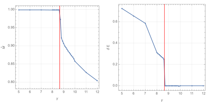
Figure 3: $\hat{M}$ and $\delta E$ are plotted as the functions of $\gamma$. The red line corresponds to the critical value $\gamma_{\rm c}\simeq 8.65$.

We can see from the right panel of Fig. 3 that our numerical solutions are reliable for $\gamma>\gamma_{\rm c}$ where the Derrick’s condition is fairly satisfied $\delta E\sim 0$, and we find from the right panel of Fig. 3 that $\hat{M}<1$ in that region, implying that the dynamical gauge field makes the mass of $k=1$ gauged anti-lump smaller than that of a BPS lump. On the other hand, for $\gamma<\gamma_{\rm c}$, the numerical solution is point-like, where $\delta E$ significantly differs from zero and thus we cannot trust our numerical solutions. Nevertheless, the behavior of the raw data of $\hat{M}$ is quite suggestive; it converges to $\hat{M}=1$, namely the point-like solutions have finite energy that coincides with the BPS lump mass. This suggests that gauged anti-lumps flow to the BPS lumps in the parameter region $\gamma<\gamma_{\rm c}$, which will be justified in the next subsection.

We show in Fig. 4 the regions where the gauged anti-lumps are regular solitonic solutions, and where they are point-like configurations (small lumps). The left panel shows the relation between the elliptic modulus $\kappa$ and $b/\alpha$ given in Eq. (4.47). The phase boundary corresponds to $\gamma=\gamma_{\rm c}=8.56$, and we have used $m_{\pi}=140$ MeV and $f_{\pi}=93$ MeV for concreteness. The right panel shows the region of regular lumps in the $\mu_{\rm B}$-$eB^{z}$ plane for various $\alpha$.

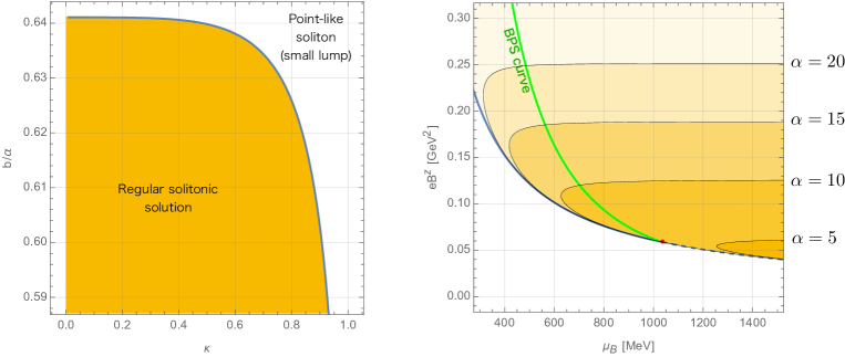
Figure 4: The phases for the regular gauged anti-lumps and point-like small anti-lumps. The left panel shows the phases in the $\kappa$-$b/\alpha$ plane. The right one shows the phases with different $\alpha$ in the $\mu_{\rm B}$-$eB^{z}$ plane. The blue solid curve at the bottom in the right panel corresponds to the CSL critical curve in Eq. (2.27), the green one corresponds to the DWSk critical curve (4.16) obtained in the BPS approximation, and the painted regions correspond to those that the anti-lump is a regular soliton. We show only relatively large $\alpha$ in $5\leq\alpha\leq 20$ because the painted region quickly move down to the far right. For example, the left tip of the painted region for $\alpha=1$ is about $\mu_{\rm B}=6.3$ GeV and 860 GeV for $\alpha=1/137$. We have used $m_{\pi}=140$ MeV and $f_{\pi}=93$ MeV for concreteness.

4.3 Small lumps and the phase diagram

Now, we are ready to reevaluate the phase boundary between the DWSk and CSL phase, which is the main result of this paper.

In the previous subsection, we have numerically investigated Eqs. (4.45) and (4.46) for the $k=1$ gauged anti-lump with the dynamical gauge field, and have found that the phase boundary between a regular soliton and a point-like soliton (small lump). Especially, we are interested in whether the anti-lump is point-like or small lump in the realistic region of $\mu_{\rm B}\sim 1$ GeV. As shown in the right panel of Fig. 4 (see also the caption), the gauged anti-lump is indeed a point-like solution for $\mu_{\rm B}\simeq 1$ GeV for the realistic value of the $U(1)_{\rm EM}$ gauge coupling: $\alpha=1/137$. However, as we mentioned above, since our numerical computations for the point-like solution are not so reliable, we analytically justify them here.

Our numerical solutions for the point-like configurations suggest that the dynamical gauge field is everywhere $a(r)=0$. Thus, we will fix $a(r)=0$, namely we will assume the dynamical gauge field is dynamically suppressed. In order to verify that the anti-lump becomes a point-like object, let us adapt the BPS anti-lump solution (Eq. (4.11) for $k=1$) with the size moduli $d_{0}$ as a variational ansatz. With respect to the $\vec{n}$ field, it is expressed as

$$n_{1}=\frac{2rd_{0}}{r^{2}+d_{0}^{2}}\cos\theta\,,\quad n_{2}=\frac{2rd_{0}}{r^{2}+d_{0}^{2}}\sin\theta\,,\quad n_{3}=\frac{r^{2}-d_{0}^{2}}{r^{2}+d_{0}^{2}}\,.$$ (4.59)

Then the kinetic energy density of $\vec{n}$ reads

$${\cal E}_{\vec{n}}=\frac{{\cal C}}{4}D_{a}\vec{n}\cdot D_{a}\vec{n}=\frac{{\cal C}}{4}\left\{\frac{8d_{0}^{2}}{\left(r^{2}+d_{0}^{2}\right)^{2}}+\frac{eB^{z}d_{0}^{2}r^{2}\left(4+eB^{z}r^{2}\right)}{\left(r^{2}+d_{0}^{2}\right)^{2}}\right\}\,.$$ (4.60)

Then, the kinetic energy can be written as

$$E_{\vec{n}}=F(\infty)-F(0)\,,$$ (4.61)

with

$$F(\rho) = \frac{\pi{\cal C}}{4}\frac{\tilde{d}_{0}^{2}}{\rho^{2}+\tilde{d}_{0}^{2}}\left\{\rho^{2}\left(\rho^{2}+2\tilde{d}_{0}^{2}\right)+2\left(\rho^{2}+\tilde{d}_{0}^{2}\right)\left(2-\tilde{d}_{0}^{2}\right)\log\frac{\rho^{2}+\tilde{d}_{0}^{2}}{eB^{z}}+4\tilde{d}_{0}^{2}\right\}$$ (4.62)

$$- \frac{\pi{\cal C}}{4}\frac{8\tilde{d}_{0}^{2}}{\rho^{2}+\tilde{d}_{0}^{2}}\,.$$

Here we have used $\tilde{d}_{0}=\sqrt{eB^{z}}\,d_{0}$. Introducing an IR cutoff $R$ ($\gg d_{0}$), we have

$$E_{\vec{n}}=2\pi{\cal C}+\frac{\pi{\cal C}eB^{z}d_{0}^{2}}{4}\left\{eB^{z}R^{2}-4\log d_{0}^{2}-2\left(2-eB^{z}d_{0}^{2}\log d_{0}^{2}\right)\right\}\,.$$ (4.63)

In the presence of the uniform magnetic field background $B^{z}>0$, this diverges in the limit $R\to\infty$ unless $d_{0}=0$. Therefore, the size of anti-lump must be 0 for $B^{z}>0$. Nevertheless, the energy remains finite even if $d_{0}=0$, and it is exactly the same as the BPS lump mass:

$$E_{\vec{n}}\big{|}_{d_{0}=0}=2\pi{\cal C}=M_{\pi}^{\rm(BPS)}\,.$$ (4.64)

This implies that the anti-lump remains as a point-like object whose energy density is

$${\cal E}_{\vec{n}}\big{|}_{d_{0}=0}=2\pi{\cal C}\delta^{(2)}(x)\,.$$ (4.65)

Including the WZW term, the total energy of the $k=1$ anti-lump is given by

$$E_{k=1}=2\pi{\cal C}-2\mu_{\rm B}\,.$$ (4.66)

Hence, the phase boundary between CSL with/without baryons coincides with that we found in the BPS approximation

$$\mu_{\rm B}\geq\frac{16\pi f_{\pi}^{2}}{3m_{\pi}}\beta(\kappa)\,,\qquad\text{for}\quad\alpha=\frac{1}{137}\,.$$ (4.67)

The phase boundary is given by the condition that the lower bound is saturated. The value of magnetic field can be determined from Eq. (2.25). We thus find the phase boundary parameterized by $\kappa$ as

$$(\mu_{\rm B},eB^{z})=\left(\frac{16\pi f_{\pi}^{2}}{3m_{\pi}}\beta(\kappa),3m_{\pi}^{2}\frac{E(\kappa)}{\kappa\beta(\kappa)}\right)\,.$$ (4.68)

We show the phase diagram in Fig. 1.

Let us make comments on comparisons with the previous studies. One should not think that this is just a repetition of the previous work Eto:2023lyo which we have reviewed in Sec. 4.2, though the final conclusion is unchanged. In the previous work Eto:2023lyo and Sec. 4.2, we have entirely ignored both the background and dynamical gauge fields for constructing the lump solutions. Then we made use of the BPS approximation and reached at the conclusion that the anti-lump is a point-like solution due to the WZW term as explained in Eq. (4.14). Especially, that result was independent of $e$ and $B^{z}$ separately but dependent of $eB^{z}$, because they only appear in the pair of $eB^{z}$ when we omit the kinetic term of the gauge field $(F_{\mu\nu})^{2}/4$ in the Lagrangian. In contrast, in this work we have refined the previous studies in Ref. Eto:2023lyo by including the dynamical gauge field $a$. We confirmed that the anti-lump is a point-like object but it is not due to the WZW term but the dynamics of the $\vec{n}$ and the gauge field. Particularly, this conclusion depends on $\alpha$ in contrast to the previous analysis. If we take a large value for $\alpha$ than $1/137$, the anti-lump could be a solitonic solution with a finite size as we will briefly discuss in the next subsection.

4.4 Properties of regular gauged anti-lump solutions

4.4.1 Baryon number and energy densities

We investigate the regular lump solutions in this subsection. For that purpose, we take $\gamma$ larger than $\gamma_{\rm c}$. We choose $\gamma=10$ as a reference value. The corresponding profiles of the numerical solution are given in Fig. 5.

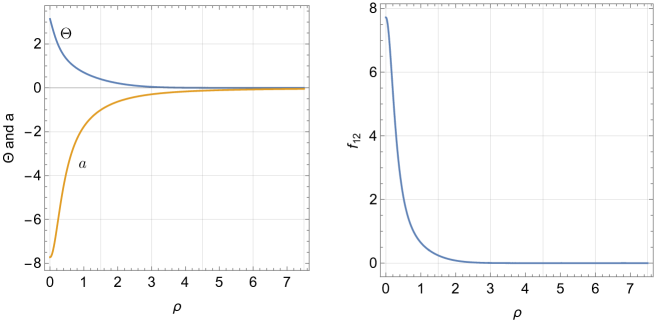
Figure 5: The profiles of the numerical solution of $k=1$ anti-lump for $\gamma=10$.

Let us also show 3 dimensional visualization of the domain-wall Skyrmions. To this end, let us first define the energy density of the CSL by substituting the CSL solution to Eq. (2.11), which can be decomposed into contributions from the chiral Lagrangian and the WZW term:

$${\cal M}_{\rm CSL}={\cal M}_{\rm CSL}^{(\Sigma)}+{\cal M}_{\rm CSL}^{\rm(WZW)}\,.$$ (4.69)

Here, the first term is a contribution from the chiral Lagrangian

$$\frac{{\cal M}^{(\Sigma)}_{\rm CSL}}{f_{\pi}^{2}m_{\pi}^{2}}=\frac{1}{2}\left(\frac{d\chi_{3}(\tilde{z})}{d\tilde{z}}\right)^{2}-\left(\cos\chi_{3}(\tilde{z})-1\right)\,,$$ (4.70)

where we have introduced $\tilde{z}=m_{\pi}z$ and $\chi_{3}(\tilde{z})=2\,{\rm am}\left(\frac{\tilde{z}}{\kappa},\kappa\right)+\pi$. The second term is a contribution from the WZW term:

$${\cal M}_{\rm CSL}^{\rm(WZW)}=\mu_{\rm B}j_{{\rm B;CSL}}^{0}$$ (4.71)

where $j_{{\rm B;CSL}}^{0}$ is the baryon charge density in Eq. (3.20), evaluated in the CSL background as

$$j_{{\rm B;CSL}}^{0}=-{\cal B}_{\rm CSL}+\tilde{\cal B}_{\rm CSL}=-\frac{eB^{z}m_{\pi}}{4\pi^{2}}\frac{d\chi_{3}(\tilde{z})}{d\tilde{z}}\,$$ (4.72)

with ${\cal B}_{\rm CSL}=0$. Then, we have

$$\frac{{\cal M}_{\rm CSL}^{\rm(WZW)}}{f_{\pi}^{2}m_{\pi}^{2}}=-\frac{4E(\kappa)}{\pi\kappa}\frac{d\chi_{3}(\tilde{z})}{d\tilde{z}}\,.$$ (4.73)

Note ${\cal M}_{\rm CSL}$ is dependent of $\tilde{z}$ only.

The total energy density ${\cal M}_{\rm DWSk}$ for the domain-wall Skyrmion can be decomposed into a contribution from the CSL background ${\cal M}_{\rm CSL}$ and one from the Skyrmion ${\cal M}_{\rm Sk}$:

$${\cal M}_{\rm DWSk}={\cal M}_{\rm CSL}+{\cal M}_{\rm Sk}\,,$$ (4.74)

which actually defines ${\cal M}_{\rm Sk}$. Then, the Skyrmion energy can be further decomposed into contributions from the chiral Lagrangian and WZW term:

$${\cal M}_{\rm Sk}={\cal M}_{\rm Sk}^{(\Sigma)}+{\cal M}_{\rm Sk}^{\rm(WZW)}\,.\quad$$ (4.75)

Here the first term is a contribution from the chiral Lagrangian

$$\frac{{\cal M}^{(\Sigma)}_{\rm Sk}}{f_{\pi}^{2}m_{\pi}^{2}} = \frac{(eB^{z})^{2}}{8\pi\alpha f_{\pi}^{2}m_{\pi}^{2}}\left[\frac{1}{4}\left\{\left(2+2a(\rho)+\rho\frac{da(\rho)}{d\rho}\right)^{2}-4\right\}\right.$$ (4.76)

$$+ \left.\frac{3\gamma}{8}\frac{\kappa K(\kappa)}{\beta(\kappa)}\left\{\left(\frac{d\Theta(\rho)}{d\rho}\right)^{2}+\frac{\left(2+\rho^{2}(1+a(\rho)\right)^{2}\sin^{2}\Theta(\rho)}{4\rho^{2}}\right\}\sin^{2}\chi_{3}(\tilde{z})\right]\,,$$

where we have used $\frac{f_{\pi}^{2}e}{B^{z}}=\frac{3\gamma}{8}\frac{\kappa K(\kappa)}{\beta(\kappa)}$. The second term is a contribution from the WZW term

$${\cal M}_{\rm Sk}^{\rm(WZW)}=\mu_{\rm B}j_{{\rm B;Sk}}^{0}\,,$$ (4.77)

where $j_{{\rm B;Sk}}^{0}$ is the baryon charge density, which can be decomposed as

$$j_{{\rm B;Sk}}^{0}=-{\cal B}_{\rm Sk}+\tilde{\cal B}_{\rm Sk}\,,$$ (4.78)

with

$${\cal B}_{\rm Sk} = -\frac{eB^{z}m_{\pi}}{4\pi^{2}}\frac{2}{\rho}\frac{d\Theta(\rho)}{d\rho}\sin\Theta(\rho)\frac{d\chi_{3}(\tilde{z})}{d\tilde{z}}\sin^{2}\chi_{3}(\tilde{z})\,,$$ (4.79)

$$\tilde{\cal B}_{\rm Sk} = \frac{eB^{z}m_{\pi}}{4\pi^{2}}\frac{1}{2}\frac{d\chi_{3}(\tilde{z})}{d\tilde{z}}\bigg{[}2\rho(1+a(\rho))\frac{d\Theta(\rho)}{d\rho}\sin\Theta(\rho)\sin^{2}\chi_{3}(\tilde{z})$$ (4.80)

$$-\left(2+2a(\rho)+\rho\frac{da(\rho)}{d\rho}\right)\cos\Theta(\rho)+2\bigg{]}\,.$$

Then we have

$$\frac{{\cal M}_{\rm Sk}^{\rm(WZW)}}{f_{\pi}^{2}m_{\pi}^{2}} = \frac{4E(\kappa)}{\pi\kappa}\left[\frac{2}{\rho}\frac{d\Theta(\rho)}{d\rho}\sin\Theta(\rho)\frac{d\chi_{3}(\tilde{z})}{d\tilde{z}}\sin^{2}\chi_{3}(\tilde{z})\right.$$ (4.81)

$$+ \frac{1}{2}\frac{d\chi_{3}(\tilde{z})}{d\tilde{z}}\bigg{\{}2\rho(1+a(\rho))\frac{d\Theta(\rho)}{d\rho}\sin\Theta(\rho)\sin^{2}\chi_{3}(\tilde{z})$$

$$\left.-\left(2+2a(\rho)+\rho\frac{da(\rho)}{d\rho}\right)\cos\Theta(\rho)+2\bigg{\}}\right].$$

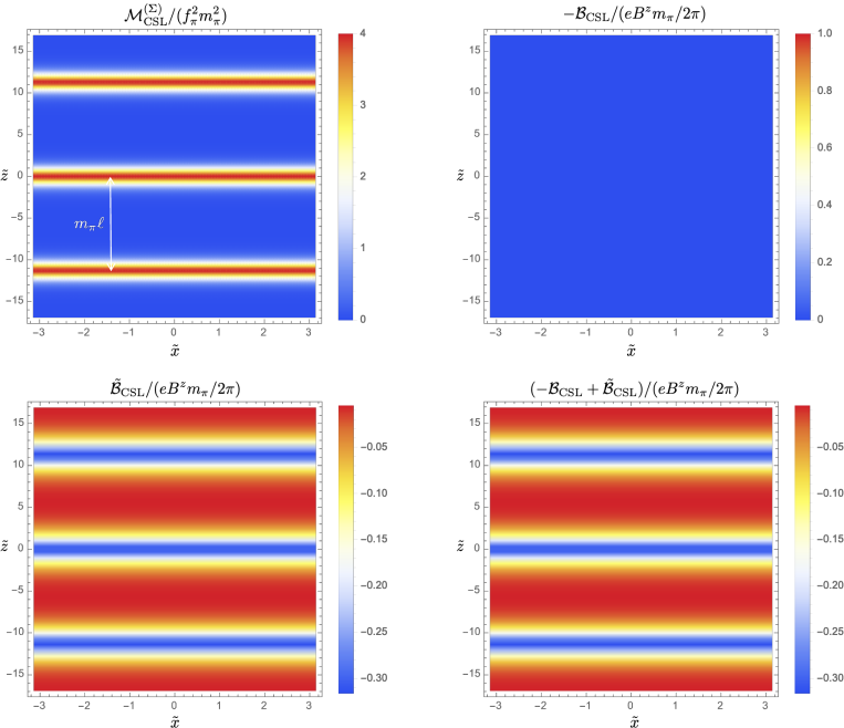
Figure 6: The cross sections at $y=0$ of dimensionless energy densities of the CSL background with $\kappa=0.9999$ ($m_{\pi}\ell=11.2892$). The kinetic energy ${\cal M}^{(\Sigma)}_{\rm CSL}$ positively contribute to the total energy density whereas the contribution of the baryon charge density $j_{\rm B;CSL}^{0}=-{\cal B}_{\rm CSL}+\tilde{\cal B}_{\rm CSL}$ from the WZW term is negative. The dimensionless coordinates are defined by $\tilde{x}=\sqrt{eB^{z}}x$ and $\tilde{z}=m_{\pi}z$.

Now we are ready to show configurations of a domain-wall Skyrmion for $\gamma=10$. We first plot in Fig. 6 a cross section at $y=0$ of contributions of the CSL to the kinetic energy ${\cal M}^{(\Sigma)}_{\rm CSL}$ and the baryon number densities $-{\cal B}_{\rm CSL}(=0)$, $\tilde{\cal B}_{\rm CSL}$ and the total baryon number density $j_{\rm B;CSL}^{0}=-{\cal B}_{\rm CSL}+\tilde{\cal B}_{\rm CSL}$. One can observe that ${\cal M}^{(\Sigma)}_{\rm CSL}$ positively contributes to the total energy density whereas the contribution of the baryon charge density $j_{\rm B;CSL}^{0}=-{\cal B}_{\rm CSL}+\tilde{\cal B}_{\rm CSL}$ from the WZW term to the total energy is negative.

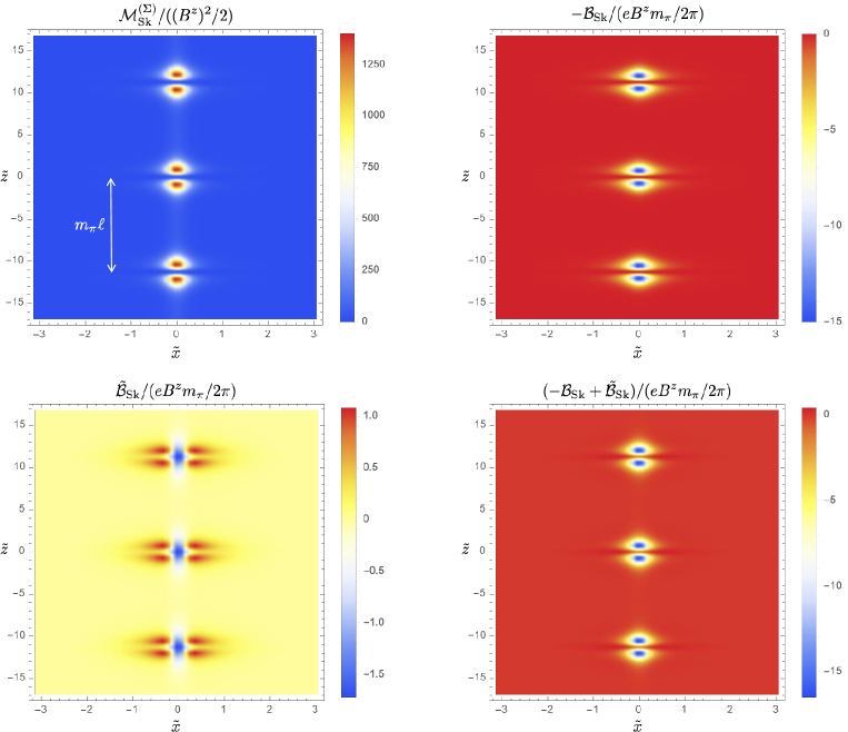
Figure 7: The cross sections at $y=0$ of dimensionless energy densities of $k=1$ anti-lump for $\gamma=10$. We take $\kappa=0.9999$ ($m_{\pi}\ell=11.2892$). The kinetic energy ${\cal M}^{(\Sigma)}$ positively contributes to the total energy density whereas the contribution of the baryon charge density $j_{\rm B}^{0}=-{\cal B}_{1}+\tilde{\cal B}_{1}$ from the WZW term is negative (The contribution of $\tilde{B}_{1}$ vanishes because of $\int d^{2}x\,\tilde{B}_{1}=0$. The dimensionless coordinates are defined by $\tilde{x}=\sqrt{eB^{z}}x$ and $\tilde{z}=m_{\pi}z$.

Next we plot in Fig. 7 contributions of a Skyrmion to the kinetic energy ${\cal M}_{\rm Sk}^{(\Sigma)}$, the baryon number densities $-{\cal B}_{\rm Sk}$, $\tilde{\cal B}_{\rm Sk}$ and the total baryon number density $j_{\rm B;Sky}^{0}=-{\cal B}_{\rm Sk}+\tilde{\cal B}_{\rm Sk}$. One can observe that ${\cal M}^{(\Sigma)}_{\rm Sk}$ positively contributes to the total energy density whereas the baryon number density $j_{\rm B;CSL}^{0}=-{\cal B}_{\rm Sk}+\tilde{\cal B}_{\rm Sk}$ from the WZW term contribute negatively to the total energy.

The superposition of the contributions from the CSL and Skyrmion gives the total baryon number and energy densities. Here, instead of do that in the 2D cross section, we show 3D plots in Fig. 8.

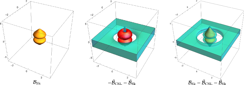
Figure 8: Isosurfaces of the baryon densities of the solitonic domain-wall Skyrmion for $\gamma=10$ and $\kappa=0.9999$. The left panel shows ${\cal B}_{\rm Sk}/(eB^{z}m_{\pi}/2\pi)=0.5$. The green and red surfaces in the middle panel correspond to $-(\tilde{\cal B}_{\rm lump}+\tilde{\cal B}_{\rm Sk})/(eB^{z}m_{\pi}/2\pi)=0.2$ and $-0.1$, respectively. The right panel shows the sum $({\cal B}_{\rm Sk}-\tilde{\cal B}_{\rm lump}-\tilde{\cal B}_{\rm Sk})/(eB^{z}m_{\pi}/2\pi)=0.5$ (inner object) and 0.25 (green outer surface). The horizontal axes are $\tilde{x}$ and $\tilde{y}$ whereas the vertical one is $\tilde{z}$.

4.4.2 Phase diagram for $\alpha=10$

Let us show the phase diagram for $\alpha=10$ in Fig. 9, though $\alpha=10$ is not realistic value.

Figure 9: The phase diagram for $\alpha=10$. The black solid curve denotes the boundary between regular (solitonic) and point-like (small) gauged anti-lumps. The region of the solitonic DWSks is further divided into those negative energy (denoted by the orange dots) and those with positive energy (denoted by the blue dots). Thus, the DWSk phase is expanded from the BPS curve (the gree solid curve) by the region with the orange dots, and the phase boundary between the DWSk and CSL phases is the red curve. The parameters are $\alpha=10$, $m_{\pi}=140$ MeV, $f_{\pi}=93$ MeV

The phase boundary beween the DWSk and CSL for $\alpha=10$ is now denoted by the red curve, where one can observe that the DWSk phase is expanded from the BPS curve (denoted by the green solid curve). The black solid curve separates the boundary regular (solitonic) and point-like (small) gauged anti-lumps. The region of the solitonic domain-wall Skyrmions is further divided into those with negative energy (denoted by the orange dots) and those with positive energy (denoted by the blue dots). In the former, gauge field dynamics lower the energy of gauged anti-lumps than the BPS lump mass. Therefore, the DWSk phase is expanded from the BPS curve.

From this case of the strong gauge coupling, one can think it to be nontrivial that the phase diagram for the realistic gauge coupling $\alpha=1/137$ is unchanged from the BPS approximation.

4.5 Gauged lumps (anti-baryons) as excited states

Let us next investigate $k=1$ lump with $N_{\rm lump}=1$ which corresponds to $N_{\rm B}^{\rm Sk}=-2$ anti-baryons. Similarly to the BPS lump discussed in Sec. 4.1.1, it is always an excited state because contribution of the WZW term to the energy density in Eq. (4.18) is positive. The Ansatz for $\Theta$ is given by

$$n_{1}=\frac{x}{r}\sin\Theta(r)\,,\quad n_{2}=-\frac{y}{r}\sin\Theta(r)\,,\quad n_{3}=\cos\Theta(r)\,.$$ (4.82)

The boundary condition for the lump in the $n_{3}=1$ vacuum is given by

$$\Theta(0)=\pi\,,\quad\Theta(\infty)=0\,,\quad\left[n_{3}(0)=-1\,,\quad n_{3}(\infty)=+1\right]\,.$$ (4.83)

The Ansatz for the dynamical gauge field $a$ is the same as Eq. (4.31). The topological charge density is given by

$$q=-\frac{\Theta^{\prime}\sin\Theta}{4\pi r}\,,$$ (4.84)

and the lump charge indeed reads

$$N_{\rm lump}=\int q\,d^{2}x=\frac{\cos\Theta(\infty)-\cos\Theta(0)}{2}=1\,.$$ (4.85)

Note that the Ansatz in Eq. (4.82) for the lump can be obtained from the Ansatz in Eq. (4.26) for the anti-lump by $n_{1}+in_{2}\to n_{1}-in_{2}$, and this is nothing but the charge conjugation $e\to-e$. Therefore, the effective Lagrangian with the lump Ansatz reads

$${\cal L}_{\rm eff}=-\frac{\ell(B^{z})^{2}}{2}\left(1+a+\frac{ra^{\prime}}{2}\right)^{2}-\frac{{\cal C}}{4}\left[\Theta^{\prime}{}^{2}+\frac{\left(2-eB^{z}r^{2}(1+a)\right)^{2}}{4r^{2}}\sin^{2}\Theta\right]\,.$$ (4.86)

Here we retain only the terms which contribute to the EOMs whereas the constant and surface terms are ignored as before. The corresponding EOMs with respect to the dimensionless variables are given by

$$\Theta^{\prime\prime}+\frac{\Theta^{\prime}}{\rho}-\frac{\left(2-\rho^{2}(1+a)\right)^{2}}{4\rho^{2}}\sin\Theta\cos\Theta=0\,,$$ (4.87)

$$a^{\prime\prime}+\frac{3a^{\prime}}{\rho}+\gamma\frac{\left(2-\rho^{2}(1+a)\right)}{2\rho^{2}}\sin^{2}\Theta=0\,.$$ (4.88)

As the anti-lump case, these include the unique parameter $\gamma$. We numerically solve the EOMs for varying $\gamma$. In contrast to the anti-lump solution, we find a regular solitonic lump for any $\gamma$. Fig. 10 shows a typical lump solution with $\gamma=5$. The magnetic flux confined at the center of the lump is negative, which is opposite to that of the anti-lump.

Figure 10: The profiles of the numerical solution of $k=1$ lump for $\gamma=5$.

The energy of the lump is a sum of $\tilde{M}_{\gamma}$ given in Eq. (4.49) and $\tilde{M}_{\pi}$ given by

$$\tilde{M}_{\pi}=\frac{4\alpha}{m_{\pi}\ell b}\frac{M_{\pi}}{m_{\pi}}=\frac{\gamma}{2}\int_{0}^{\infty}d\rho\,\rho\left[\Theta^{\prime}{}^{2}+\frac{\left(2-\rho^{2}(1+a)\right)^{2}}{4\rho^{2}}\sin^{2}\Theta\right]\,.$$ (4.89)

This is slightly different from Eq. (4.50). Furthermore, $\tilde{E}^{(4)}$ and $\tilde{E}^{(0)}$ in the Derrick’s condition are same as those given in Eqs. (4.53) and (4.55) whereas $\tilde{E}^{(1)}$ differs from Eq. (4.54) and it is given by

$$\tilde{E}^{(1)}=\frac{4\alpha}{m_{\pi}\ell b}E^{(1)}=\frac{\gamma}{2}\int d\rho\,\rho\left(-1+\frac{a\rho^{2}}{2}\right)\sin^{2}\Theta\,.$$ (4.90)

Figure 11: $\hat{M}$ and $\delta E$ are plotted as the functions of $\gamma$ for a lump (anti-baryon in the bulk).

We show $\hat{M}$ and $\delta E$ given in Eq. (4.58) for the gauged lump in Fig. 11. One can see from the left panel that the lump energy is less than the BPS lump energy for any $\gamma$, and can check from the right panel that the Derrick’s theorem is well satisfied in the whole region of $\gamma$. This is in contrast to the case of the gauged anti-lumps (baryons) in Fig. 3 in which the Derrick’s theorem is satisfied only above the critical value $\gamma$.

5 Summary and Discussion

We have studied the phase diagram of QCD at finite baryon density with strong magnetic fields. We have found that the phase boundary between the CSL and DWSk phases previously obtained in the BPS approximation is unchanged beyond the BPS approximation taking into account the dynamics of the gauge field. We also have found that the domain-wall Skyrmions are electrically charged with the charge one as a result of the chiral anomaly. For realistic value of the gauge coupling the anti-lumps in the domain-wall effective theory (baryons in the bulk) becomes small lumps of zero size but are still physical with finite energy, implying that the phase boundary is unchanged from the BPS curve. On the other hand, at strong gauge coupling their solutions become regular and their energy is smaller than BPS lump mass, implying that the phase boundary changes from the BPS curve as the DWSk phase expands as in Fig. 9. While gauged anti-lumps can have negative energy due to the WZW term in the DWSk phase, gauged lumps (anti-baryons in the bulk) are regular and have positive energy in any parameter regions.

Let us make comments on future directions. In this paper, we mainly concentrated on single gauged (anti-)lumps for the purpose of determining the phase boundary between the DWSk and CSL phases. In order to see a structure of DWSk phase, one has to discuss multiple gauged anti-lumps and investigate interaction among them. When there are more than one anti-lumps, the limit of zero size modulus allows finite size anti-lumps. In order to have a Skyrmion crystal, anti-lumps must feel repulsion. From our previous work Amari:2024adu on gauged lumps in the background magnetic field, (anti-)lumps seem to feel attraction (when the WZW term is neglected). However, as shown in this paper, anti-lumps are electrically charged due to the WZW term. Thus, we can expect a Skyrmion crystal on the soliton.

In this paper, we have used the moduli approximation, that does not include a back reaction from the Skyrmions to the solitons. It is an important future problem to construct full three dimensional solutions of domain-wall Skyrmions, including a Skyrmion lattice structure mentioned above.

When the isospin chemical potential is introduced, the charged pions are condensed in the ground state. In such a case, there appears a vortex-Skyrmion phase Qiu:2024zpg , where a vortex-Skyrmion is a Skyrmion hosted by a vortex rather than a domain wall Gudnason:2014hsa ; Gudnason:2014jga ; Gudnason:2016yix . It is an open question how the vortex-Skyrmion phase and domain-wall Skyrmion phase are connected in a phase diagram spaned by the isospin chemical potential.

One of future directions is a generalization to $N_{\rm F}$ flavors. In such a case, the effective theory on the soliton is the ${\mathbb{C}}P^{N_{\rm F}-1}$ model. Skyrmions in the ${\mathbb{C}}P^{2}$ model ($N_{\rm F}=3$) with Dzyaloshinskii-Moriya interaction were studied recently Akagi:2021dpk ; Amari:2022boe .