Pathfinder for Low-altitude Aircraft with Binary Neural Network

Abstract

A prior global topological map (e.g., the OpenStreetMap, OSM) can boost the performance of autonomous mapping by a ground mobile robot. However, the prior map is usually incomplete due to lacking labeling in partial paths. To solve this problem, this paper proposes an OSM maker using airborne sensors carried by low-altitude aircraft, where the core of the OSM maker is a novel efficient pathfinder approach based on LiDAR and camera data, i.e., a binary dual-stream road segmentation model. Specifically, a multi-scale feature extraction based on the UNet architecture is implemented for images and point clouds. To reduce the effect caused by the sparsity of point cloud, an attention-guided gated block is designed to integrate image and point-cloud features. For enhancing the efficiency of the model, we propose a binarization streamline to each model component, including a variant of vision transformer (ViT) architecture as the encoder of the image branch, and new focal and perception losses to optimize the model training. The experimental results on two datasets demonstrate that our pathfinder method achieves SOTA accuracy with high efficiency in finding paths from the low-level airborne sensors, and we can create complete OSM prior maps based on the segmented road skeletons. Code and data are available at: https://github.com/IMRL/Pathfinder.

I INTRODUCTION

In recent years, autonomous mapping based on ground robots has become a popular research area [1, 2]. Existing methods can generally work well in small areas with simple topology but usually fail in large scenes [3, 4, 5, 6]. To solve this problem, some mapping methods guided by prior global maps have been proposed, such as based on the GPS coordinates of Open Street Maps (OSM)  [1, 7, 8]. With prior global information, robots can plan an optimal path to follow and complete the mapping on a large scale. However, prior maps are usually incomplete due to the loss of GPS signals or the lack of labelling in OSM (as shown in Fig.1). Thus, robots cannot scout every corner of the scene even if they follow the planned path according to the prior map.

This work addresses this issue by proposing an OSM maker using airborne sensors (LiDAR and camera). The OSM maker can generate an entire topology of traversable road networks and provide the complete prior OSM map required to guide ground robots in autonomous mapping, acting as a mapping assistant for ground robots in a cooperative mapping framework [9, 10, 11]. Like any real-time mapping and robotic exploration algorithms, the OSM maker should be as efficient as possible given the low-cost and power-efficiency requirements. Thus, we propose a novel efficient binary dual-stream road segmentation model, where weights and activations are represented with only 1 bit. For 1-bit weights and activations, Xnor and PopCount operations [12] can replace floating-point multiplication and addition (MAC) operations, significantly reducing memory requirements and computational costs. To our best knowledge, it is the first binary dual-stream model that effectively fuses RGB images and LiDAR point-cloud data for road segmentation tasks, not limited to applications to low-altitude aircraft. The contributions of this work are summarized as follows:

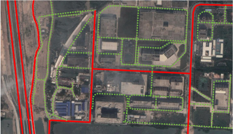
Figure 1: OpenStreetMap Road Network on Satellite Imagery. The red lines represent the OSM roads. The areas where roads are absent from the OSM (GPS coordinates) data are marked with green dashed lines.

• We propose an OSM maker to automatically generate a complete OSM prior map for collaborative (ground-robot and low-altitude drone) robot mapping at a large scale.

• We propose a novel binary dual-stream framework, Binarized Pathfinder, of accurate and efficient road segmentation for OSM generation.

• To optimize the model training process, we design a new variant of focal loss to mitigate the adverse effects of class imbalance on road segmentation tasks.

II RELATED WORK

II-A Road segmentation

Road segmentation from aerial-view images can be categorized into traditional-based and deep learning-based. The early methods are based on manually designed features  [13, 14, 15]. Generally, these methods are not robust to variations in lighting and contrast [16]. In contrast, deep-learning methods have performed better due to their powerful representation ability. RoadNet [17] was proposed to extract road surfaces, but its speed and accuracy were not optimal. To overcome this issue, FCN replaced fully connected layers with deconvolution to achieve per-pixel classification, resulting in improved performance in road segmentation tasks [18]. To effectively utilize multi-scale information, UNet was applied in road segmentation [19]. Most recently, the method based on the Deeplab network [20] adopted dilated convolutions and pyramid pooling layers to capture long-range information and preserve spatial structures, respectively.

Additionally, effective LiDAR-based point cloud segmentation methods have also been proposed, which can be divided into direct methods [21] and projection-based methods [22]. In direct methods, such as RandLA-Net [21], which processes the point cloud directly without any data format conversion and applies clustering to improve the segmentation efficiency. In contrast, projection methods convert 3D point clouds into 2D images (such as bird’s-eye views) to leverage efficient 2D convolutional networks for enhancing real-time processing capabilities [22].

Image-based approaches may experience performance degradation in adverse conditions, while point clouds obtained by Lidar suffer from sparsity issues. Combining the advantages of different types of sensors has made fusion methods more promising [23, 24]. IKD-Net [23] mined imbalance information across modalities to extract features from heterogeneous multimodal data comprising aerial images and LiDAR.

Due to operational efficiency and power consumption limitations, it should be noted that current methods are essentially unsuitable for edge devices such as drones. Therefore, more efficient methods such as Binary Neural Network (BNN) based methods are necessary.

II-B Binary Neural Network

Network binarization [12, 25, 26] is the most extreme form of network quantization [27, 28], in which weights and activations are quantized to 1 bit [12]. Compared to full-precision networks, binarized models suffer from reduced accuracy due to the limited representational capacity of features and the non-differentiability of binary functions. To address this problem, various methods have been proposed to mitigate the negative impact of network binarization and improve performance without significantly increasing computational complexity. BNN [12] is the first method that fully binarizes CNN weight and activations and applies Xnor and PopCount operations to simplify full precision matrix multiplication. Xnor-Net [29] adds scaling factors to the weights and activations to enhance the performance of BNN on large datasets. By adding learnable thresholds before the sign function and incorporating RPReLU activation functions after each residual connection, ReActNet [26] further improves the performance of BNN in large datasets with the reshaped output distribution. In the ViT domain, BHViT [25] demonstrates the incompatibility between the ViT structure and binarization techniques and proposes the first binarized hybrid ViT model. BiViT [30] proposes a mixed-precision ViT approach, where the activations in the MLP are full-precision, but the weights of all the attention and MLP modules are binary. Binary-DAD-Net [31] fully binarizes the DeeplabV3 network of full precision, marking the first BNN tailored for image-based road segmentation tasks.

III METHOD

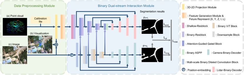
Figure 2: The general Structure of proposed network

The general structure of our proposed network is depicted in Fig.2. Binarized Pathfinder is a typical dual-stream architecture, including an image branch and a point-cloud one. Each branch is a UNet composed of the encoder and decoder based on a pyramid structure (four stages with different feature resolutions). For each stage of the decoder, the feature from the corresponding stage of the encoder is passed through a residual link and added together. To solve the problem caused by the sparsity of the point cloud, at each stage of the encoder, we fuse image features with point cloud features using a fusion module. Additionally, we propose a new road detection dataset, the Lidar-visual-fusion dataset for road segmentation (RS-LVF), based on the MARS-LVIG dataset [32] for the road segmentation task. To accomplish feature alignment and the data fusion of the point cloud and image, we use the BEV projection [22] to map sparse 3D point clouds in the 2D camera coordinate system.

III-A Binary Convolution Unit

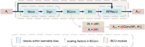
Figure 3: The figure of the convolution process of Binary Convolution Unit (BCU)

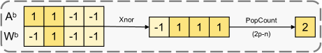
Figure 4: The Xnor and PopCount operations. PopCount counts the number of ”1”s (the sum of 1) in the result vector of the Xnor operation (consisting of -1 and 1). $p$ and $u$ mean the number of 1 and -1, respectively. And the vector length $n=p+u$. we can replace the dot product result from $p-u$ to $p-(n-p)=2p-n$.

The Binary Convolution Unit (BCU) [26] (shown in Fig. 3) with the binary convolution layer could be represented as:

$$A_{i+1}=bcov\left(\alpha W_{i}^{b},\beta A_{i}^{b}\right)\approx\alpha\beta\cdot\varphi\left(W_{i}^{b},A_{i}^{b}\right),$$ (1)

where $W_{i}^{b}=\mathrm{sign}\left(W_{i}\right)$ with $W_{i}$ being the full-precision weight. $A_{i}^{b}=\mathrm{sign}\left(A_{i}\right)$ and $A_{i}$ is the full-precision activation. The $\mathrm{sign}$ is a thresholding operation. $\varphi$ is the Xnor-PopCount operation, shown in Fig.4, which can theoretically result in a 64 $\times$ reduction of the required inference time [29] compared to matrix multiplication with full precision. $\alpha$ and $\beta$ are scale factors for weight and activation, respectively. The scale factor enables the estimated binary weights and activations to approximate the full-precision weights and activations, as indicated by $W_{i}\approx\alpha W_{i}^{b}$ and $A_{i}\approx\beta A_{i}^{b}$.

To address the non-differentiability of the sign function, we apply the sub-gradient method [33], straight-through estimator (STE), as below

$$\frac{\partial}{\partial x}\text{sign}\left(x\right)\approx\left\{\begin{array}[]{l}1\ \ \ \ |x|<1\\ 0\ \ \ \ \text{otherwise}\\ \end{array}\right..$$ (2)

To improve the performance of binary networks, following ReaAct-Net [26], we apply the residual connection to improve the activation information. Meanwhile, we apply learnable biases in sign and activation to mitigate gradient mismatch by adjusting the activation distribution [26].

III-B Binary Encoder for Feature Extraction

Attention-guided Gating Block (AGB): The sparsity of the point cloud makes the corresponding feature maps exhibit numerous voids, represented by dark hues in column 5 of Fig. 9. To mitigate these voids, we propose an attention-guided gating module to generate the weight to fuse image features with point cloud features, as shown in Fig. 5. Let the image features be $Q_{i}\in\mathbb{R}^{C_{i}~{}\times H_{i}~{}\times W_{i}}$, where $i~{}\in[1,2,3,4]$ is the index of the encoder stage. Similarly, let $P_{i}^{2d}~{}\in~{}\mathbb{R}^{C_{i}~{}\times~{}H_{i}~{}\times~{}W_{i}}$ represent the features of the projected point cloud. The AGB module comprises fusion and attention map modules with the operational formula as follows

$$F_{i}^{fu} =f_{i}^{bcu}\left(\varUpsilon\left(P_{i}^{2d},Q_{i}\right)+P_{i}^{2d}+Q_{i}\right),$$ (3)

$$F_{i}^{out} =P_{i}^{2d}+\sigma\left(F_{i}^{fu}+\eta\left(f_{i}^{bcu}\left(F_{i}^{fu}\right)\right)\right)\odot F_{i}^{fu},$$

where $F_{i}^{fu}$ is the output of fusion module. $f_{i}^{bcu}$ is the binary convolution unit mentioned in Section III-A. $\varUpsilon$ indicates the operation that concatenates the image and lidar features along the channel dimension. $F_{i}^{out}$ means the output of the AGB block. $\sigma$ means a sigmoid function and $\eta$ represents the batch-norm layer.

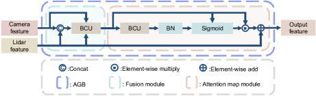
Figure 5: Depiction of the Attention-Guided Gated Block (AGB): The AGB integrates features from both the camera and LIDAR, effectively augmenting the deficient areas in the original LIDAR feature representation. $BN$ is the batch normalization layer. $Concat$ is the operation that concatenates two feature maps along the channel dimension.

LiDAR Encoder: The LIDAR stream encoder comprises Binary-ResBlocks, as shown in Fig. 6, with four different resolutions of the feature map. The architecture of a Binary-ResBlock consists of three BCUs. The shortcut added layer by layer mitigates the gradient mismatch [26] issue. The outcomes of the three BCUs are aggregated and averaged to produce output1 for residual connections to the decoder. Subsequently, an average pooling layer is applied to reduce the resolution of output1 by half as output2 for further processing. To balance performance and efficiency, we apply the shallow-ResBlock with full precision, containing only one 1x1 convolution and two convolution units, for the initial feature extraction stage of the point cloud.

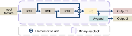
Figure 6: Description of feature Process in a Binary-resblock

Binary Atrous Spatial Pyramid Pooling block (Binary-ASPP): The block consists of four binary dilated convolution units with different dilation rates ($d=\{1,6,12,18\}$). These units each output feature maps of the same size. For processing these feature maps in a binarization-friendly way, different from the architecture of the original ASPP module, we replace the 1$\times$1 convolution layer with add and average operation to produce the final output. We add the bottleneck module Binary-ASPP within the LiDAR stream, which can adjust the feature map with lowest spatial resolution obtained from the encoder to enhance feature representation.

Camera Encoder: The camera encoder is a multi-scale binarized CNN-ViT hybrid model. We apply a shallow feature extraction network using convolutional modules to minimize computational complexity, while a deeper network utilizing ViT block focuses on capturing comprehensive features. Meanwhile, this approach addresses the problem of significant information loss associated with binarizing multiscale feature extraction frameworks. The image encoder operates through multiple downsampling modules that halve the size of the feature map at each layer, which helps to preserve critical details and reduces the loss of essential features. The CNN module applies a variant of ASPP named Multi-scale Binary dilated convolution Block (MBB, Fig.7) for the shallow network component. Meanwhile, this module retains substantial global and local information without increasing computational complexity, thereby enhancing overall performance.

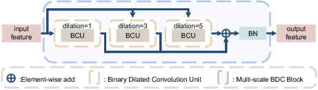
Figure 7: The Multi-scale Binary Dilated Convolution Block(MBB)

III-C Binary Decoder for Segmentation

The LiDAR stream decoder utilizes the same binary ResBlock as the corresponding encoder. To avoid introducing additional computation, we applied pixel shuffle to perform upsampling, which only rearranges features without additional operations. Compared with bilinear upsampling, pixel shuffle is particularly suitable for BNN. For the camera stream decoder, we adopt a pyramid structure based on four binary ResNet blocks, with the resolution increasing by two times at each layer.

III-D Loss Function

We employ four types of losses, including focal loss [34], variant focal loss, Lovász loss [35], and pixel-level interaction loss, denoted by $L_{foc}$, $L_{vf}$, $L_{lo}$ and $L_{pi}$, respectively. In particular, the $L_{vf}$ is a new loss designed based on the focal loss (Eq. 4), through which we aim to gradually reduce the contribution of easy samples to the overall loss in a simulated annealing style. Basically, in the later training stages, the optimization focuses mainly on hard samples.

$$L_{vf} =\frac{1}{C\!\!\times\!\!H\!\!\times\!\!W}\underset{c=1}{\overset{C}{\sum{}}}\underset{i=1}{\overset{H\times W}{\sum{}}}f^{mask}\!\cdot\!\hat{a}^{c}\!\!\cdot\!\left(-\left(1-p^{c}_{i}\right)^{\hat{\delta}}\log\left(p^{c}_{i}\right)\right),$$ (4)

where $C$ is the number of classes, and $H$ and $W$ represent the height and width of the feature map, respectively. $f^{mask}$ is the void mask with 0 values corresponding to the void areas of the point cloud. The $\hat{a}^{c}$ and $\hat{\delta}$ are defined as

$$\hat{a}^{c} =\left\{\begin{array}[]{l}a_{0}^{c}\ \ \ ep\leq\frac{ep_{t}}{10},\\ a_{0}^{c}-\frac{\left(a_{0}^{c}-1\right)\left(10\cdot ep-ep_{t}\right)}{ep_{t}\cdot\left(\lambda-1\right)+\varepsilon}\ \ \ \frac{ep_{t}}{10}<ep\leq ep_{t}\cdot\frac{\lambda}{10}\\ 1\ \ \ \ \ \text{otherwise}\\ \end{array}\right.,$$ (5)

$$\hat{\delta} =\left\{\begin{array}[]{l}2\ \ \ \ ep\leq\frac{ep_{t}}{10}\\ 0\ \ \ \ \text{otherwise}\\ \end{array}\right.,$$

where $\lambda$ is a hyperparameter, set 2 in the experiment. $\varepsilon$ is a small nonzero number. $ep$ is the current epoch index and $ep_{t}$ is the number of total epochs. $a_{0}^{c}=\frac{N_{total}}{N_{c}}$, with $N_{total}$ and $N_{c}$ being the number of total samples and the number of samples of class $c$, respectively.

Meanwhile, we introduce $L_{pi}$ (Eq. 6), a pixel-level interaction loss inspired by knowledge distillation techniques, which involves calculating the Kullback-Leibler divergence of the prediction results. Specifically, we utilize the overlapping predicted results of the image feature maps and the void area of point-cloud feature maps as soft labels, which can guide the corresponding areas in the point-cloud feature maps to enhance the overall performance.

$$L_{pi}=\frac{1}{H\times W}\,\,\underset{i=1}{\overset{H\times W}{\sum{}}}\left(f^{mask}\right)^{-1}KL\left(F_{i}^{pcd}||F_{i}^{img}\right),$$ (6)

where $KL(\cdot||\cdot)$ is the Kullback-Leibler divergence. $F_{i}^{pcd}$ and $F_{i}^{img}$ represent the confidence map of the LiDAR stream and camera stream, respectively. Above all, the total loss is $L_{total}=L_{pi}+L_{foc}+L_{lo}^{pcd}+L_{vf}+L_{lo}^{img}$, where $L_{lo}^{pcd}$ and $L_{lo}^{img}$ are the Lovász loss applied to the LiDAR stream and camera stream, respectively.

III-E The post-processing of OSM maker

In this subsection, we briefly introduce the post-processing of the OSM maker, shown in Fig.8. The homogeneity matrix between successive frames is estimated for image stitching. Each road segmentation map is warped according to the corresponding homography matrix to concatenate with the previous one. Then, a skeleton extraction algorithm [36] is applied to extract the topological structure. In practical applications, the stitched map is aligned automatically with the existing OSM road skeleton based on a registration algorithm. Then, with interpolation of GPS coordinates, we can obtain a complete OSM map.

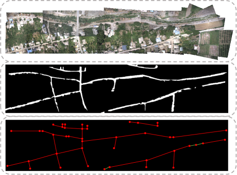
Figure 8: The OSM maker. From top to bottom, image matching, road segmentation, and topology extraction, respectively. The green line in third row is the result of road breakpoint completion.

IV EXPERIMENTS AND RESULTS

IV-A Benchmark Datasets

RS-LVF Dataset:

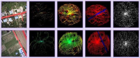
Figure 9: The pictures from left to right are aerial images(with red labels), point clouds in a single frame, Point clouds accumulated over multi-frames(one second), point cloud labels, and point cloud projected onto image plane showing the void, respectively. The black regions in the fifth column of the figure denote the area without point data, reflecting the typical characteristics of non-re-scanning solid-state LiDAR data. Compared with the second column, the accumulated point cloud data shown in the third column is denser.

Despite numerous UAV aerial image datasets, outdoor scene datasets with multi-modal data and a downward-looking perspective are still lacking for our task. One suitable existing dataset that satisfies our requirement is the AMtown part of MARS-LVIG dataset [32], whose point cloud data are collected by a non-rescanning solid-state LIDAR data with a limited FOV (e.g., the DJI-mid360 [37]). However, this dataset lacks semantic annotation, and each frame of the point cloud is too sparse. Thus, we create a dataset, Lidar-visual-fusion dataset for road segmentation(RS-LVF), from the AMtown part of MARS-LVIG dataset to fulfil our road segmentation task. Totally, our dataset includes 960 pairs of LIDAR point clouds, RGB images, LiDAR-camera calibration files, and semantic annotations. Fig.9 shows two samples. To solve the problem that the point cloud of the MARS-LVIG dataset is too sparse, we obtain frames of relatively dense point clouds by accumulating multiple sparse point cloud frames within one-second intervals based on the odometry estimated by FastLIO2 [38].

SensatUrban Dataset: Generated by drone photogrammetry, SensatUrban [39] is a color-labeled point cloud dataset on the city scale. The dataset contains three billion points with rich semantic labels (categorized into 13 classes). To ensure fairness in comparisons, we follow the official partitioning strategy to train our method.

IV-B Training Procedure and Performance Metrics

Training Procedure: For data augmentation, we apply the random color jitter to the image data. To train our model, we use the SGD optimizer with cosine annealing learning-rate decay, an initial learning rate of 0.001 and a batch size of 2 for the camera stream. Meanwhile, we utilize the AdamW optimizer with an initial learning rate set of 0.0005 for the LIDAR stream. We train our model with 100 epochs in the RS-LVF dataset. For the SensatUrban dataset, we train our model with 300 epochs.

Performance Metrics: We use the Mean Intersection over Union (mIOU) metric to evaluate segmentation performance, measuring the overlap area of each class between the predicted segmentation and the ground truth: $mIoU=\frac{1}{n}\underset{c=1}{\overset{n}{\sum{}}}\frac{TP_{c}}{TP_{c}+FP_{c}+FN_{c}}$, where $TP_{c}$ means true positives for class $c$, $FP_{c}$ and $FN_{c}$ mean the false positives and false negatives, respectively.

IV-C Results

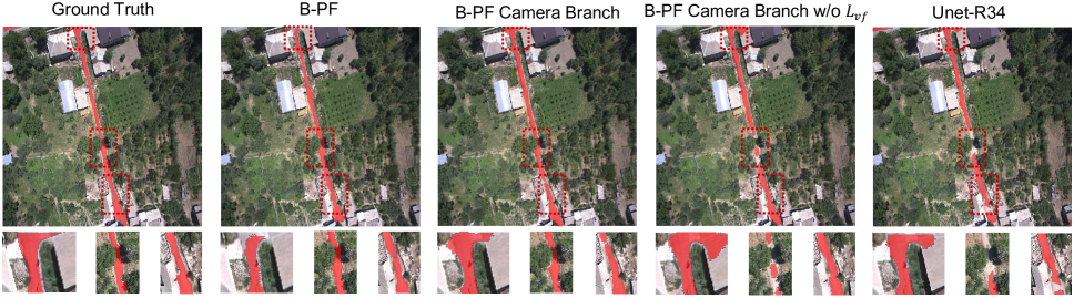
Figure 10: Quantitative results on different scenarios in RS-LVF dataset. B-PF is an abbreviation for Binarized Pathfinder.

TABLE I: Comparison results of road segmentation in RS-LVF dataset. ’I’ is image and ’P’ refers point cloud.

Method	Input	Pre-trained	Point Cloud				Image
			mAcc	mIou	Road Acc	Road Iou	mAcc	mIou	Road Acc	Road Iou
SalsaNext [40]	P	✕	78.73	67.18	60.49	39.51	$-$	$-$	$-$	$-$
UNet R34 [22]	I	$\checkmark$	$-$	$-$	$-$	$-$	85.36	77.76	72.06	58.41
PMF [24]	I & P	$\checkmark$	95.12	90.47	91.28	82.19	81.36	76.54	63.62	56.54
Ours(FP)	I & P	$\checkmark$	95.55	91.23	91.72	83.60	93.36	86.57	87.62	74.67
Ours(binary)	I & P	✕	94.61	90.19	89.87	81.69	92.23	85.13	85.43	71.98

Results on RS-LVF: As shown in Tab. I, our proposed method achieves SOTA performance among various methods trained on the RS-LVF dataset. Without fine-tuning, the proposed full-precision method achieves 91.23$\%$ point cloud mIOU and 86.57$\%$ image mIOU on the RS-LVF dataset. Compared with the corresponding full-precision network, the precision of the binary method decreases by 0.77$\%$ point cloud mIOU and 1.44$\%$ image mIOU, respectively. As shown in Fig. 10, some qualitative results illustrate that integrated point cloud features have a better discriminative ability for roads with shadows or roofs with textures similar to roads.

Results on SensatUrban: To comprehensively evaluate the proposed algorithm, we utilize a multi-class segmentation dataset, the SensatUrban dataset, to compare the binarized pathfinder model with other SOTA methods. As shown in Table II, the full-precision pathfinder achieves the best performance compared to the other method. Compared to the corresponding full-precision network, the accuracy of our binarized pathfinder model decreased by 2.6$\%$.

TABLE II: Comparison results of Semantic Segmentation in SensatUrban dataset.Highlight the highest value using bold font, and the second highest using underline.

Method	mIOU	Ground	Veg.	Build.	Wall	Bri.	Park.	Rail	Traffic	Street	Car	Foot	Water
									road	road
RandLA-Net [21]	52.69	80.11	98.07	91.58	48.88	40.75	51.62	0.00	56.67	33.23	80.14	32.63	71.31
KPConv [41]	57.58	87.10	98.91	95.33	74.40	28.69	41.38	0.00	55.99	54.43	85.67	40.39	86.30
UNet-R34 [22]	59.90	78.45	95.39	97.89	60.72	59.80	40.45	40.35	67.32	51.42	82.11	41.94	62.87
MVP-Net [42]	59.40	85.10	98.50	95.90	66.00	57.50	52.70	0.00	61.90	49.70	81.80	43.90	78.20
LACV-Net [43]	61.30	85.50	98.40	95.60	61.90	58.60	64.00	28.50	62.80	45.40	81.90	42.40	67.70
NLA-GCL-Net [44]	56.40	$-$	$-$	$-$	$-$	$-$	$-$	$-$	$-$	$-$	$-$	$-$	$-$
Ours(FP)	62.65	82.77	97.70	96.15	74.71	42.96	40.99	58.22	65.50	54.84	85.71	37.43	77.57
Ours(binary)	60.03	82.78	97.31	95.34	77.44	11.53	45.65	62.82	62.32	55.33	87.18	35.33	67.32

IV-D Ablation Study

Effect of Network Components: Sufficient ablation experiments are conducted to assess the effectiveness of each proposed module. We individually remove each module from the proposed binarized pathfinder model to observe performance variations on the RS-LVF dataset. The results are presented in Tab. III, demonstrating that each proposed module has effectively improved the network performance. The baseline represents our proposed algorithm stripped of the mentioned modules. $mIOU^{*}$ is the average mIOU of the point cloud and the image. Specifically, the difference of $mIOU^{*}$ between the fifth row and the last row of Tab. III illustrates the effectiveness of the proposed loss $L_{vf}$. The quantitative result (shown in Fig. 10) demonstrates that the proposed loss can recognize hard samples.

TABLE III: Performance metrics for different models and classes. ”Bi-ASPP” refers to utilizing the optimized version of ASPP to instead the original binary ASPP.

Baseline	AGB	Bi-ASPP	$L_{Pi}$	$L_{vf}$	$mIOU$
					LiDAR	Img	All
$\checkmark$					62.65	83.81	73.2
$\checkmark$	$\checkmark$				87.83	84.98	86.4
$\checkmark$		$\checkmark$			63.31	83.77	73.6
$\checkmark$	$\checkmark$		$\checkmark$		88.79	85.04	86.9
$\checkmark$	$\checkmark$	$\checkmark$	$\checkmark$		89.46	84.84	87.2
$\checkmark$	$\checkmark$	$\checkmark$		$\checkmark$	89.18	85.10	87.1
$\checkmark$	$\checkmark$	$\checkmark$	$\checkmark$	$\checkmark$	90.19	85.13	87.8

TABLE IV: Computational complexity for different models. G is $10^{9}$ and the image size is 512 $\times$ 512

Network	Flops (G)	Bops (G)	Ops (G)	Para.(MB)
PMF-Net (FP)	237.71	0	237.71	138.90
Ours (FP)	202.28	0	202.28	153.69
Ours (binary)	13.46	188.82	16.41	15.24

Effect of binarization: Following ReAct-Net [26], we utilize the OPs ($OPs=BOPs/64+FLOPs$) to evaluate the complexity of binary neural networks. BOPs and FLOPs represent binary operations and floating-point operations, respectively. As shown in the Tab. IV, the binarization process decreases the OPs of Pathfinder from 202.28 G to 16.41 G. The memory requirement is also decreased from 153.69 MB to 15.24 MB.

V CONCLUSIONS

In this paper, we propose an OSM maker to tackle the problem, labelling lacking in partial paths, within the current OSM method. A key component of our approach is an efficient binary dual-stream road segmentation model built on the Unet architecture. To boost the performance of our model, we employ improved loss functions and specially designed modules for method optimization. Experimental results demonstrate that our approach attains state-of-the-art accuracy (mIOU) while maintaining low memory usage and computational complexity in finding path, which ensures the capability of OSM maker to complete or maintain high-precision OSM prior maps efficiently.

References

- [1] W. Gao, Z. Sun, M. Zhao, C.-Z. Xu, and H. Kong, “Active loop closure for osm-guided robotic mapping in large-scale urban environments,” 2024.
- [2] H. Qin, Z. Meng, W. Meng, X. Chen, H. Sun, F. Lin, and M. H. Ang, “Autonomous exploration and mapping system using heterogeneous uavs and ugvs in gps-denied environments,” IEEE Transactions on Vehicular Technology, vol. 68, no. 2, pp. 1339–1350, 2019.
- [3] Z. Sun, B. Wu, C. Xu, and H. Kong, “Concave-hull induced graph-gain for fast and robust robotic exploration,” IEEE Robotics and Automation Letters, 2023.
- [4] A. Das, M. Diu, N. Mathew, C. Scharfenberger, J. Servos, A. Wong, J. S. Zelek, D. A. Clausi, and S. L. Waslander, “Mapping, planning, and sample detection strategies for autonomous exploration,” Journal of Field Robotics, vol. 31, no. 1, pp. 75–106, 2014.
- [5] B. P. L. Lau, B. J. Y. Ong, L. K. Y. Loh, R. Liu, C. Yuen, G. S. Soh, and U.-X. Tan, “Multi-agv’s temporal memory-based rrt exploration in unknown environment,” IEEE Robotics and Automation Letters, vol. 7, no. 4, pp. 9256–9263, 2022.
- [6] A. Patel, S. Karlsson, B. Lindqvist, C. Kanellakis, A.-A. Agha-Mohammadi, and G. Nikolakopoulos, “Towards energy efficient autonomous exploration of mars lava tube with a martian coaxial quadrotor,” Advances in Space Research, vol. 71, no. 9, pp. 3837–3854, 2023.
- [7] M. Hentschel and B. Wagner, “Autonomous robot navigation based on openstreetmap geodata,” International IEEE Conference on Intelligent Transportation Systems, pp. 1645–1650, 2010.
- [8] M. Á. Muñoz-Bañón, E. Velasco-Sanchez, F. A. Candelas, and F. Torres, “Openstreetmap-based autonomous navigation with lidar naive-valley-path obstacle avoidance,” IEEE Transactions on Intelligent Transportation Systems, vol. 23, no. 12, pp. 24 428–24 438, 2022.
- [9] I. D. Miller, F. Cladera, T. Smith, C. J. Taylor, and V. Kumar, “Stronger together: Air-ground robotic collaboration using semantics,” IEEE Robotics and Automation Letters, vol. 7, no. 4, pp. 9643–9650, 2022.
- [10] ——, “Air-ground collaboration with spomp: Semantic panoramic online mapping and planning,” IEEE Transactions on Field Robotics, pp. 1–1, 2024.
- [11] Y. Yue, C. Zhao, Z. Wu, C. Yang, Y. Wang, and D. Wang, “Collaborative semantic understanding and mapping framework for autonomous systems,” IEEE/ASME Transactions on Mechatronics, vol. 26, no. 2, pp. 978–989, 2021.
- [12] I. Hubara, M. Courbariaux, D. Soudry, R. El-Yaniv, and Y. Bengio, “Binarized neural networks,” in Advances in Neural Information Processing Systems, D. Lee, M. Sugiyama, U. Luxburg, I. Guyon, and R. Garnett, Eds., vol. 29, 2016.
- [13] S. Valero, J. Chanussot, J. A. Benediktsson, H. Talbot, and B. Waske, “Advanced directional mathematical morphology for the detection of the road network in very high resolution remote sensing images,” Pattern Recognition Letters, vol. 31, no. 10, pp. 1120–1127, 2010.
- [14] J. Yuan and A. M. Cheriyadat, “Road segmentation in aerial images by exploiting road vector data,” Fourth International Conference on Computing for Geospatial Research and Application, pp. 16–23, 2013.
- [15] Y. Shao, B. Guo, X. Hu, and L. Di, “Application of a fast linear feature detector to road extraction from remotely sensed imagery,” IEEE Journal of Selected Topics in Applied Earth Observations and Remote Sensing, vol. 4, no. 3, pp. 626–631, 2010.
- [16] I. Kahraman, I. Karas, and A. E. Akay, “Road extraction techniques from remote sensing images: A review,” The International Archives of the Photogrammetry, Remote Sensing and Spatial Information Sciences, vol. 42, pp. 339–342, 2018.
- [17] Y. Liu, J. Yao, X. Lu, M. Xia, X. Wang, and Y. Liu, “Roadnet: Learning to comprehensively analyze road networks in complex urban scenes from high-resolution remotely sensed images,” IEEE Transactions on Geoscience and Remote Sensing, vol. 57, no. 4, pp. 2043–2056, 2018.
- [18] R. Kestur, S. Farooq, R. Abdal, E. Mehraj, O. Narasipura, and M. Mudigere, “Ufcn: A fully convolutional neural network for road extraction in rgb imagery acquired by remote sensing from an unmanned aerial vehicle,” Journal of Applied Remote Sensing, vol. 12, no. 1, pp. 016 020–016 020, 2018.
- [19] X. Yang, X. Li, Y. Ye, R. Y. K. Lau, X. Zhang, and X. Huang, “Road detection and centerline extraction via deep recurrent convolutional neural network u-net,” IEEE Transactions on Geoscience and Remote Sensing, vol. 57, pp. 7209–7220, 2019.
- [20] L.-C. Chen, Y. Zhu, G. Papandreou, F. Schroff, and H. Adam, “Encoder-decoder with atrous separable convolution for semantic image segmentation,” in European Conference on Computer Vision (ECCV), 2018, pp. 801–818.
- [21] Q. Hu, B. Yang, L. Xie, S. Rosa, Y. Guo, Z. Wang, N. Trigoni, and A. Markham, “Randla-net: Efficient semantic segmentation of large-scale point clouds,” in IEEE/CVF Conference on Computer Vision and Pattern Recognition (CVPR), 2020, pp. 11 105–11 114.
- [22] Z. Zou and Y. Li, “Efficient urban-scale point clouds segmentation with bev projection,” 2021.
- [23] Y. Wang, Y. Wan, Y. Zhang, B. Zhang, and Z. Gao, “Imbalance knowledge-driven multi-modal network for land-cover semantic segmentation using aerial images and lidar point clouds,” ISPRS Journal of Photogrammetry and Remote Sensing, vol. 202, pp. 385–404, 2023.
- [24] Z. Zhuang, R. Li, K. Jia, Q. Wang, Y. Li, and M. Tan, “Perception-aware multi-sensor fusion for 3d lidar semantic segmentation,” in IEEE/CVF International Conference on Computer Vision (ICCV), 2021, pp. 16 260–16 270.
- [25] T. Gao, C.-Z. Xu, and H. Kong, “Bhvit: Binarized hybrid vision transformer based on multi-scale feature fusion,” 2024.
- [26] Z. Liu, Z. Shen, M. Savvides, and K.-T. Cheng, “Reactnet: Towards precise binary neural network with generalized activation functions,” in European Conference on Computer Vision (ECCV), A. Vedaldi, H. Bischof, T. Brox, and J.-M. Frahm, Eds., 2020, pp. 143–159.
- [27] S. Han, H. Mao, and W. J. Dally, “Deep compression: Compressing deep neural network with pruning, trained quantization and huffman coding,” arXiv: Computer Vision and Pattern Recognition, 2015.
- [28] H. Qin, R. Gong, X. Liu, X. Bai, J. Song, and N. Sebe, “Binary neural networks: A survey,” Pattern Recognition, vol. 105, p. 107281, 2020.
- [29] M. Rastegari, V. Ordonez, J. Redmon, and A. Farhadi, “Xnor-net: Imagenet classification using binary convolutional neural networks,” in ECCV, B. Leibe, J. Matas, N. Sebe, and M. Welling, Eds., 2016, pp. 525–542.
- [30] Y. He, Z. Lou, L. Zhang, J. Liu, W. Wu, H. Zhou, and B. Zhuang, “Bivit: Extremely compressed binary vision transformers,” in IEEE/CVF International Conference on Computer Vision, 2023, pp. 5651–5663.
- [31] A. Frickenstein, M.-R. Vemparala, J. Mayr, N.-S. Nagaraja, C. Unger, F. Tombari, and W. Stechele, “Binary dad-net: Binarized driveable area detection network for autonomous driving,” in IEEE International Conference on Robotics and Automation (ICRA), 2020, pp. 2295–2301.
- [32] H. Li, Y. Zou, N. Chen, J. Lin, X. Liu, W. Xu, C. Zheng, R. Li, D. He, F. Kong et al., “Mars-lvig dataset: A multi-sensor aerial robots slam dataset for lidar-visual-inertial-gnss fusion,” The International Journal of Robotics Research, p. 02783649241227968, 2024.
- [33] S. Boyd, L. Xiao, and A. Mutapcic, “Subgradient methods,” lecture notes of EE392o, Stanford University, Autumn Quarter, vol. 2004, no. 01, 2003.
- [34] T.-Y. Lin, P. Goyal, R. Girshick, K. He, and P. Dollár, “Focal loss for dense object detection,” in IEEE International Conference on Computer Vision, 2017, pp. 2980–2988.
- [35] M. Berman, A. R. Triki, and M. B. Blaschko, “The lovász-softmax loss: A tractable surrogate for the optimization of the intersection-over-union measure in neural networks,” in IEEE conference on computer vision and pattern recognition, 2018, pp. 4413–4421.
- [36] D. Bulatov, S. Wenzel, G. Häufel, and J. Meidow, “Chain-wise generalization of road networks using model selection,” ISPRS Annals of the Photogrammetry, Remote Sensing and Spatial Information Sciences, vol. 4, pp. 59–66, 2017.
- [37] “Livox mid-360 user manual.” [Online]. Available: https://www.livoxtech.com/mid-360/downloads
- [38] W. Xu, Y. Cai, D. He, J. Lin, and F. Zhang, “Fast-lio2: Fast direct lidar-inertial odometry,” IEEE Transactions on Robotics, vol. 38, no. 4, pp. 2053–2073, 2022.
- [39] Q. Hu, B. Yang, S. Khalid, W. Xiao, N. Trigoni, and A. Markham, “Sensaturban: Learning semantics from urban-scale photogrammetric point clouds,” International Journal of Computer Vision, vol. 130, no. 2, pp. 316–343, 2022.
- [40] T. Cortinhal, G. Tzelepis, and E. Erdal Aksoy, “Salsanext: Fast, uncertainty-aware semantic segmentation of lidar point clouds,” in Advances in Visual Computing: 15th International Symposium, 2020, pp. 207–222.
- [41] H. Thomas, C. Qi, J.-E. Deschaud, B. Marcotegui, F. Goulette, and L. J. Guibas, “Kpconv: Flexible and deformable convolution for point clouds,” IEEE/CVF International Conference on Computer Vision (ICCV), pp. 6410–6419, 2019.
- [42] H. Li, H. Guan, L. Ma, X. Lei, Y. Yu, H. Wang, M. R. Delavar, and J. Li, “Mvpnet: A multi-scale voxel-point adaptive fusion network for point cloud semantic segmentation in urban scenes,” International Journal of Applied Earth Observation and Geoinformation, vol. 122, p. 103391, 2023.
- [43] Z. Zeng, Y. Xu, Z. Xie, W. Tang, J. Wan, and W. Wu, “Lacv-net: Semantic segmentation of large-scale point cloud scene via local adaptive and comprehensive vlad,” ArXiv, vol. abs/2210.05870, 2022.
- [44] J. Wang, W. Fan, X. Song, G. Yao, M. Bo, and Z. Liu, “Nla-gcl-net: semantic segmentation of large-scale surveying point clouds based on neighborhood label aggregation (nla) and global context learning (gcl),” International Journal of Geographical Information Science, 2024.