Finite Sample Analysis of Distribution-Free Confidence Ellipsoids for Linear Regression

Abstract

The least squares (LS) estimate is the archetypical solution of linear regression problems. The asymptotic Gaussianity of the scaled LS error is often used to construct approximate confidence ellipsoids around the LS estimate, however, for finite samples these ellipsoids do not come with strict guarantees, unless some strong assumptions are made on the noise distributions. The paper studies the distribution-free Sign-Perturbed Sums (SPS) ellipsoidal outer approximation (EOA) algorithm which can construct non-asymptotically guaranteed confidence ellipsoids under mild assumptions, such as independent and symmetric noise terms. These ellipsoids have the same center and orientation as the classical asymptotic ellipsoids, only their radii are different, which radii can be computed by convex optimization. Here, we establish high probability non-asymptotic upper bounds for the sizes of SPS outer ellipsoids for linear regression problems and show that the volumes of these ellipsoids decrease at the optimal rate. Finally, the difference between our theoretical bounds and the empirical sizes of the regions are investigated experimentally.

I Introduction

Building mathematical models of unknown systems based on noisy empirical data is a fundamental problem in system identification, signal processing and machine learning. There are several standard methods that provide point estimates with uncertainty quantification based on limiting distributions. Typical examples include prediction error methods [1] with asymptotic confidence regions derived from the central limit theorem. A considerable disadvantage of these confidence sets is that they are only approximately correct for finite samples. Consequently, their application could be problematic in domains with strong stability or safety requirements.

In order to overcome this issue, a substantial amount of the recent research in system identification focus on approaches with non-asymptotic guarantees [2]. One of the most common techniques to derive probability approximately correct (PAC) bounds for an estimate, such as LS, is based on the theory of concentration inequalities, which induces confidence regions.

Several works analyzed (closed-loop) dynamical systems, where the sample complexity of transition matrix estimations were studied for fully observable [3] and also non-observable state space settings [4]. A signal processing focused approach was investigated in [5], where a low-rank and structured sparse high-dimensional vector autoregressive (VAR) system was analyzed, and a new estimation technique was proposed with non-asymptotic probabilistic upper bounds on the estimation error. In the aforementioned works, there are strong assumptions on the noises, namely that they follow some specific distribution, in most cases they are Gaussian. Another limitation is that the confidence regions heavily rely on specific constants (hyper-parameters), which are coming from the assumptions on the system setting and the distributions of the inputs and the outputs. In practice, these hyper-parameters are usually unknown and only estimates can be used or bounds based on domain specific knowledge of experts. For finite impulse response (FIR) systems, PAC bounds for the LS estimate were given in [6], under a centered subgaussian noise assumption. Despite the relaxed noise assumption compared to the Gaussian case, building confidence regions using this results would still rely on the variance proxy of the subgaussian distribution.

It is also possible to work with alternative loss functions, such as the Chebyshev loss (i.e., the $\ell_{\infty}$ case). Assuming uniformly distributed (therefore bounded) noises, PAC bounds can be derived for the Chebyshev estimate, as well [7].

Set membership identification is another class of methods that can provide quality tags for point estimates in the form of bounding ellipsoids [8]. These approaches usually also consider (closed-loop) dynamical systems, however, some of their variants address FIR models assuming that only quantized [9] of even binary [10] measurements are available. In most cases of set membership identification, bounded noises are assumed, where the bound is typically assumed to be known a priori, though some recent works estimate it from the data [11].

As both set membership identification and statistical learning theory [12] based confidence region constructions require strong assumptions and a priori knowledge about the noises affecting the systems, algorithms that can build confidence regions in a distribution-free and data-driven (hyper-parameter-free) way for any finite sample size are highly desirable.

Two identification algorithms that satisfy these properties (i.e., non-asymptotic, distribution-free and data-driven) are the LSCR: Leave-out Sign-dominant Correlation Regions [13] and the SPS: Sign-Perturbed Sums [14] methods. They also have several distributed signal processing applications, including source localization in wireless sensor networks [15], and distributed evaluation of confidence sets [16]. In [15] LSCR confidence regions were built to characterize the search space of the source parameters, while [16] proposed an SPS-based diffusion algorithm to avoid flooding the network.

In this paper, we further study the SPS method, which can construct exact, non-asymptotic confidence regions for the true system parameters under the assumption that the noises are independent and symmetric about zero. SPS was originally introduced for general linear systems [17], but apart from its exact coverage probability, many of its theoretical guarantees are for linear regression models with independent regressors [14]. By using instrumental variables, several properties of SPS can be generalized to closed-loop state space models [18].

Theoretical guarantees besides exact coverage were rigorously proven for SPS, such as uniform strong consistency[19], which means that the SPS regions almost surely shrink around the true parameters, as the sample size increases. This result however is asymptotic, and the finite sample performance of SPS remained an open question until recently. In our previous work [20], we have investigated the sample complexity of SPS for linear regression problems, i.e., we have derived non-asymptotic PAC bounds for the volumes of SPS regions. We have also shown that the sizes of SPS regions decrease at an optimal rate $\mathcal{O}(1/\sqrt{n})$, where $n$ is the sample size.

All of the theoretical results mentioned above considers the fundamental construction of SPS: the indicator function. The standard SPS, given by its indicator function, is a hypothesis test that checks whether a given parameter is included in the confidence region. Using the indicator function to determine all the points of the confidence set would be computationally demanding, therefore in [14] an ellipsoidal outer approximation (EOA) algorithm was proposed, which gives a compact representation of the SPS region. An important feature of the constructed ellipsoid is that its center and shape matrix coincide with that of the confidence ellipsoid constructed using the classical asymptotic theory, only its radius is different. This radius, which ensures finite sample guarantees, can be computed in polynomial time, by solving semidefinite optimization problems. The EOA construction of SPS was later generalized to ARX [21] and closed-loop state space models [18], as well.

In this we work provide a finite sample analysis of the EOA of SPS for general linear regression problems with exogenous regressors, e.g., for FIR systems. We prove high probability upper bounds on the sizes of the resulting confidence ellipsoids. Our analysis builds on some results from the sample complexity analysis of standard SPS regions [20], however, we analyse the finite sample properties of a convex semidefinite program, which requires a significantly different approach than deriving concentration inequalities for the indicator function. We also show that the obtained bounds are “close” to the bounds of the original SPS region and that they decrease at the optimal rate, that is, $\mathcal{O}(1/\sqrt{n})$. Simulation experiments that demonstrate the difference between our theoretical bounds and the empirical sizes of the regions are also presented. We emphasize that although our analysis use distribution and regressor dependent parameters, the SPS EOA does not require these parameters, and it can be applied under very general assumptions, unlike standard non-asymptotic solutions, for example, based on PAC bounds or set membership ellipsoids.

II Problem setting

This section introduces the addressed linear regression problem and presents our main assumptions. Note that the same assumptions are used as for the sample complexity analysis of the SPS-Indicator function (Algorithm 2) [20].

II-A Data Generation

Consider the following linear regression problem

$$Y_{t}\,\doteq\,\varphi_{t}^{\mathrm{T}}\theta^{*}+W_{t},$$ (1)

for $t\in[n]\doteq\{1,\dots,n\}$, where $Y_{t}$ is the scalar output, $\varphi_{t}$ is a $d$-dimensional deterministic regressor, $\theta^{*}$ is the $d$-dimensional (constant) true parameter and $W_{t}$ is the (random) scalar noise. We are given a sample of size $n$ which consists of $\varphi_{1},\dots,\varphi_{n}$ (input vectors) and $Y_{1},\dots,Y_{n}$ (noisy, scalar outputs).

The following notation will be used throughout the paper:

$$\Phi_{n}\doteq\begin{bmatrix}\varphi_{1}^{\mathrm{T}}\\ \varphi_{2}^{\mathrm{T}}\\ \vdots\\ \varphi_{n}^{\mathrm{T}}\end{bmatrix},\qquad w_{n}\doteq\begin{bmatrix}W_{1}\\ W_{2}\\ \vdots\\ W_{n}\end{bmatrix},\qquad y_{n}\doteq\begin{bmatrix}Y_{1}\\ Y_{2}\\ \vdots\\ Y_{n}\end{bmatrix},$$ (2)

$$R_{n}\doteq\sum_{t=1}^{n}\varphi_{t}\varphi_{t}^{\mathrm{T}}=\Phi_{n}^{\mathrm{T}}\Phi_{n},\quad\bar{R}_{n}\doteq\frac{1}{n}R_{n}.$$ (3)

In our analysis we focus on deterministic regressor sequences $\{\varphi_{t}\}$, however, our results can be straightforwardly generalized to random exogenous regressors, i.e., regressors that are independent of the noise sequence $\{W_{t}\}$. In order to do that the assumptions on the regressors A2-A4 must be satisfied almost surely and the derivations can be traced back to the presented one by fixing a realization of the regressors.

II-B Assumptions

Our core assumptions are the following:

A1.

The noise sequence $\{W_{t}\}$ is independent and contains nonatomic, $\sigma$-subgaussian random variables whose probability distributions are symmetric about zero.

An (integrable) random variable $W$ is $\sigma$-subgaussian[22, Definition 2.2], if for all $\lambda\in\mathbb{R},$ there is a $\sigma>0$, such that

$$\mathbb{E}\big{[}\exp(\lambda(W\!-\mathbb{E}[W]))\big{]}\,\leq\,\exp\!{\left(\frac{\lambda^{2}\sigma^{2}}{2}\right)}.$$ (4)

Note that the quantity $\sigma^{2}$ is often referred to as the variance proxy. Naturally, any Gaussian random variable with variance $\sigma^{2}$ is $\sigma$-subgaussian. Furthermore, any distribution with a bounded support on $[a,b]$ is subgaussian with $\sigma=(b-a)/2$ [22, Example 2.4]. Standard examples of such distributions include the uniform, the triangular and the beta distributions.

Recall that random variable $W$ is called symmetric about zero if  $W$ has the same probability distribution as $-W$. Finally, a random variable $W$ is called nonatomic, if for all constant $w\in\mathbb{R}$, it holds that $\mathbb{P}(W=w)=0.$ Notice that every continuous probability distribution is nonatomic.

Our assumptions on the noises are rather mild, since the subgaussian assumption covers a wide range of possible distributions, furthermore, the noise sequence can even be nonstationary, i.e., their distributions can change over time. The nonatomicity of the distributions is only assumed to simplify the analysis, by using proper random tie-breaking in the SPS Outer Approximation algorithm (Algorithm 3), such as step 3 of Algorithm 2, the assumption could be relaxed.

A2.

The regressor vectors are “completely exciting” in the sense that any $d$ regressors span the whole space, $\mathbb{R}^{d}$.

This means that for any subset  $T$ of the index set $[n]$ with $|\hskip 1.13809ptT\hskip 0.56905pt|=d$, hence, having cardinality $d$, we have that

$$\det\!\left(\frac{1}{d}\sum_{t\in T}\varphi_{t}\varphi_{t}^{\mathrm{T}}\right)\,\neq\,0.$$ (5)

A2 ensures under suitable assumptions on the perturbations (step 3 of Algorithm 1), that the SPS confidence regions, including the outer approximation regions, are bounded.

A3.

The excitations are nonvanishing in the sense that there exists a constant  $\lambda_{0}>0$, such that for all  $n\geq d:$

$$\lambda_{\text{min}}(\bar{R}_{n})\,\geq\,\lambda_{0}\,>\,0,$$ (6)

where  $\lambda_{\text{min}}$ denotes the smallest eigenvalue.

Assumption A3 guarantees that the averaged “magnitude” of the excitation does not get too small, hence it provides a lower bound on the signal-to-noise ratio.

A4.

Let  $\Phi_{n}=\Phi_{{\scriptscriptstyle Q},n}\Phi_{{\scriptscriptstyle R},n}$ be the thin QR-decomposition of  $\Phi_{n}$. There are constants $\kappa>0$ and  $0<\rho\leq 1$, such that the following upper bound holds for all  $n\geq d,$ we have

$$\mu(\Phi_{n})\,\doteq\,\frac{n}{d}\max_{1\leq i\leq n}\left\lVert\Phi_{{\scriptscriptstyle Q},n}^{\mathrm{T}}e_{i}\right\rVert^{2}\leq\,\kappa\,n^{1-\rho},$$ (7)

where $\mu(\Phi_{n})$ is called the coherence of  $\Phi_{n}$.

A4 applies the definition of coherence from [23, Definition 1.2] along with the facts that $\text{range}(\Phi_{n})=\text{range}(\Phi_{{\scriptscriptstyle Q},n})$ and $\Phi_{{\scriptscriptstyle Q},n}\Phi_{{\scriptscriptstyle Q},n}^{\mathrm{T}}$ is an orthogonal projection onto $\text{range}(\Phi_{n})$. A consequence of this is that $1\leq\mu(\Phi_{n})\leq n/d$ [23]. This assumption provides an upper bound on how much of the excitation can be “concentrated” to a single time step, i.e., onto a particular regressor $\varphi_{t}$. In the presented theorems A4 will be assumed alongside with A2, hence, the thin QR-decomposition of $\Phi_{n}=\Phi_{{\scriptscriptstyle Q},n}\Phi_{{\scriptscriptstyle R},n}$ is unique, since matrix $\Phi_{{\scriptscriptstyle R},n}$ is full rank.

If the regressors are realizations of i.i.d. continuous random vectors with a positive definite covariance matrix, then it can be shown that the aforementioned assumptions are almost surely satisfied. More rigorously, if the distribution is continuous, then it does not concentrate to any proper affine subspace, hence A2 is satisfied, furthermore, since the regressors are i.i.d., the excitations (a.s.) do not vanish (A3) and (a.s.) satisfy the coherence assumption (A4) with some $\rho$ and $\kappa$, as well.

Realizations of i.i.d. continuous variables as input or as regressors are very common in signal processing practice. Typical examples are the continuous white noise or filtered white noise, with a $d$-ranked matrix FIR or IIR filter.

The SPS EOA algorithm, presented as Algorithm 3, requires much milder assumptions on the noises and regressors. The introduced stronger assumptions are needed to analyse the size of the constructed confidence ellipsoids for any finite sample size and almost all realizations of the regressor vectors.

III The Sign-Perturbed Sums method

This section overviews the original SPS algorithm and its ellipsoidal outer approximation. The intuitive idea behind SPS, detailed descriptions of the algorithms and the proofs of the presented theorems can be found in [14] and [20].

III-A The SPS-Indicator algorithm

The SPS method consists of two parts. The first part is the initialization, where given the desired confidence probability $p$, the algorithm computes the global variables and generates the required random objects, including the random signs. The SPS-Initialization is given in Algorithm 1. The second part is the indicator function, which decides whether the input parameter $\theta$ is included in the confidence region. The SPS-Indicator is presented in Algorithm 2. Using this construction, the $p$-level SPS confidence region can be defined as

$$\mathcal{C}_{p,n}\,\doteq\,\{\,\theta\in\mathbb{R}^{d}\text{ : SPS-Indicator}(\theta)=1\,\}.$$ (8)

Algorithm 1 Pseudocode: SPS-Initialization ($p$)

1:  Given the (rational) confidence probability $p\in(0,1)$, set integers $m>q>0$ such that $p=1-q/m$.

2:  Calculate the outer product $\bar{R}_{n}$ and find the principle square root $\bar{R}_{n}^{1/2}$, such that

$$\bar{R}_{n}^{1/2}\bar{R}_{n}^{{1/2}}=\bar{R}_{n}.$$

3:  Generate $n\cdot(m-1)$ i.i.d. random signs $\{\alpha_{i,t}\}$ for $i\in[\hskip 0.85358ptm-1\hskip 0.56905pt]$ and $t\in[\hskip 0.85358ptn\hskip 0.56905pt]$, with:

$$\mathbb{P}(\alpha_{i,t}=1)\,=\,\mathbb{P}(\alpha_{i,t}=-1)\,=\,1/2.$$

4:  Generate (uniformly) a random permutation $\pi$ of the set $\{0,\dots,m-1\}$, where each of the $m!$ possible permutations has probability $1/(m!)$ to be selected.

Algorithm 2 Pseudocode: SPS-Indicator $(\theta)$

1:  Compute the prediction errors for $\theta:$ for $t\in[\hskip 0.85358ptn\hskip 0.56905pt]$ let

$$\varepsilon_{t}(\theta)\,\doteq\,Y_{t}-\varphi_{t}^{\mathrm{T}}\theta.$$

2:  Evaluate for $i\in[\hskip 0.85358ptm-1\hskip 0.56905pt]$ the following functions:

$$S_{0}(\theta)\,\doteq\,\bar{R}_{n}^{-\frac{1}{2}}\frac{1}{n}\sum_{t=1}^{n}\varphi_{t}\varepsilon_{t}(\theta),$$

$$S_{i}(\theta)\,\doteq\,\bar{R}_{n}^{-\frac{1}{2}}\frac{1}{n}\sum_{t=1}^{n}\alpha_{i,t}\varphi_{t}\varepsilon_{t}(\theta).$$

3:  Compute the rank of $\left\lVert S_{0}(\theta)\right\rVert^{2}$ among $\{\left\lVert S_{i}(\theta)\right\rVert^{2}\}:$

$$\mathcal{R}(\theta)\,\doteq\,\left[\,1+\sum_{i=1}^{m-1}\mathbb{I}\left(\left\lVert S_{0}(\theta)\right\rVert^{2}\succ_{\pi}\left\lVert S_{i}(\theta)\right\rVert^{2}\right)\,\right]\!,$$

where “$\succ_{\pi}$” is “$>$” with random tie-breaking, i.e., $\left\lVert S_{k}(\theta)\right\rVert^{2}\succ_{\pi}\left\lVert S_{j}(\theta)\right\rVert^{2}$ if and only if $(\left\lVert S_{k}(\theta)\right\rVert^{2}>\left\lVert S_{j}(\theta)\right\rVert^{2})\lor(\left\lVert S_{k}(\theta)\right\rVert^{2}=\left\lVert S_{j}(\theta)\right\rVert^{2}\,\land\,\pi(k)>\pi(j))$.

4:  Return 1 if  $\mathcal{R}(\theta)\leq m-q$, otherwise return 0.

It is proved in [14] that the confidence region $\mathcal{C}_{p,n}$ covers the true parameter $\theta^{*}$ with exact probability $p$, under general assumptions on the noise and regressor sequences, which are much milder than A1-A4, hence the following theorem holds.

Theorem 1.

Assuming the noise sequence $\{W_{t}\}$ contains independent random variables that are symmetric about zero and matrix $\bar{R}_{n}$ is nonsingular, the coverage probability of the constructed confidence region is exactly $p$, that is,

$$\mathbb{P}(\theta^{*}\in\mathcal{C}_{p,n})=1-\frac{q}{m}=p.\vspace{1mm}$$ (9)

It has been also rigorously proven that these confidence regions are strongly consistent [19], which requires some further assumptions on the regressor sequence. The sample complexity of the SPS-Indicator algorithm was studied in [20]. The following theorem provides high probability upper bounds for the diameters of the confidence regions generated by the SPS-Indicator algorithm for finite sample sizes $n$.

Theorem 2.

Assume A1, A2, A3 and A4. Then, the following concentration inequality holds for the diameters of SPS sets. For all $\delta\in(0,1)$ and  $n\geq\lceil g^{1/\rho}(\frac{\delta}{m-q})\rceil,$ we have

$$\!\!\!\sup_{\theta_{1},\theta_{2}\in\mathcal{C}_{p,n}}\!\!\!\!\|\,\theta_{1}-\theta_{2}\,\|\,\leq\,\dfrac{4\,f\!\left(\frac{\delta}{m-q}\right)}{\left(n^{1-\rho}\lambda_{0}\!\left(n^{\rho}-g\!\left(\frac{\delta}{m-q}\right)\right)\right)^{\frac{1}{2}}},\vspace{1mm}$$ (10)

with probability at least  $1-\delta,$ where

$$f(\delta)\,\doteq\,\begin{cases}\sigma\hskip 0.85358pt(\hskip 0.85358pt8\hskip 1.42262ptd\ln^{\frac{1}{2}}(\tfrac{4}{\delta})+d)^{\frac{1}{2}}&4e^{-(nd\lambda_{0})^{2}}\leq\delta\leq 2,\\[2.84526pt] \sigma\left(8\ln(\tfrac{4}{\delta})+d\right)^{\frac{1}{2}}&0<\delta<4e^{-(nd\lambda_{0})^{2}},\\ \end{cases}$$

$$g(\delta)\,\doteq\,\ln\left(\tfrac{4d}{\delta}\right)2\hskip 0.85358pt\kappa\hskip 0.85358ptd^{2}.$$ (11)

III-B The SPS ellipsoidal outer approximation

Observe that the SPS-Indicator algorithm detailed in Section III-A only checks whether a given parameter $\theta$ is included in the confidence region. Building a confidence region using this indicator function requires to evaluate every point on a grid, which is computationally demanding. To give a compact representation of the confidence region around the least squares estimate (LSE) that can be efficiently computed, an ellipsoidal outer approximation (EOA) method was developed, see [14]. The confidence region given by this outer approximation is

$$\mathcal{C}_{p,n}\,\subseteq\,\mathcal{O}_{p,n}\,\doteq\bigl{\{}\hskip 0.85358pt\theta\in\mathbb{R}^{d}:(\theta-\hat{\theta}_{n})^{\mathrm{T}}{\bar{R}_{n}}(\theta-\hat{\theta}_{n})\leq r\hskip 0.85358pt\bigl{\}},\vspace{1mm}$$ (12)

where $\hat{\theta}_{n}\doteq R_{n}^{-1}\Phi_{n}^{\mathrm{T}}y_{n}$ is the LSE and $r$ can be computed from the solutions of the following optimization problems:

$$\max_{\theta} \left\lVert S_{0}(\theta)\right\rVert^{2}$$ (13)

s.t. $$\left\lVert S_{0}(\theta)\right\rVert^{2}-\left\lVert S_{i}(\theta)\right\rVert^{2}\leq 0,$$

$i\in[\hskip 0.85358ptm-1\hskip 0.56905pt]$. The precise computation of $r$ and the SPS outer approximation are detailed in Algorithm 3. The optimization problems (13) are not convex in general, however they can be reformulated to convex semidefinite programs (SDP), which can be solved in polynomial time [14]. A detailed description of the these SDP reformulations are given in Section IV. As $\mathcal{O}_{p,n}$ is the sought outer approximation, it satisfies that

$$\mathbb{P}(\theta^{*}\in\mathcal{O}_{p,n})\geq 1-\frac{q}{m}=p.$$ (14)

Algorithm 3 Pseudocode: SPS Outer Approximation

1:  Compute the least-squares estimate,

$$\hat{\theta}_{n}=R_{n}^{-1}\Phi_{n}^{\mathrm{T}}y_{n}.$$

2:  For $i\in[\hskip 0.85358ptm-1\hskip 0.56905pt]$, solve the optimization problem (13), and let $\gamma_{i}^{*}$ be the optimal value.

3:  Let $r$ be the $q$th largest $\gamma_{i}^{*}$ value.

4:  The outer approximation of the SPS confidence region is given by the ellipsoid

$$\mathcal{O}_{p,n}\,\doteq\bigl{\{}\hskip 0.85358pt\theta\in\mathbb{R}^{d}:(\theta-\hat{\theta}_{n})^{\mathrm{T}}{\bar{R}_{n}}(\theta-\hat{\theta}_{n})\leq r\hskip 0.85358pt\bigl{\}}.$$

IV Sample complexity of the
SPS Ellipsoidal Outer Approximation

The SPS ellipsoid gives a compact representation of the confidence region, and compared to applying the SPS-Indicator, it can be much more easily used in various applications, from robust optimization to risk management. It is also significantly less demanding from a computational point of view, as it can be computed in polynomial time. The following theorem formalizes the sample complexity of these ellipsoids, i.e., it shows how their radii shrink as the sample size increases.

Theorem 3.

Assuming A1, A2, A3 and A4, the following concentration inequality holds for the sizes of SPS ellipsoidal outer approximation confidence regions. For all  $\delta\in(0,1)$ and  $n\geq\lceil g^{1/\rho}(\frac{\delta}{m-q})\rceil$ with probability at least  $1-\delta,$ we have

$$\sup_{\theta\in\mathcal{O}_{p,n}}\|\theta-\hat{\theta}_{n}\|\leq\dfrac{2f(\frac{\delta}{m-q})(n^{\frac{\rho}{2}}+g^{\frac{1}{2}}(\frac{\delta}{m-q}))^{\frac{1}{2}}}{\left(n\lambda_{0}(n^{\frac{\rho}{2}}-g^{\frac{1}{2}}(\frac{\delta}{m-q}))\right)^{\frac{1}{2}}}.$$ (15)

Notice that unlike in Theorem 2, the size of the region is expressed as the distance between any point in the region and the LSE, which is the center of the outer ellipsoid, see (12). The functions $f(\delta)$ and $g(\delta)$ are defined in (2), and, as in Theorem 2, they are independent of the sample size, $n$.

Comparing the sample complexities of the SPS-Indicator and SPS EOA, it can be observed from Theorems 2 and 3 that the SPS EOA is more conservative, however, the difference is not significant. This behavior is a consequence of the construction, it is expected that an outer approximation has a slightly worse sample complexity. Despite this, as shown in the following corollary, the shrinkage rates of both algorithms are the same, which makes the SPS EOA optimal, since apart from constant factors, this rate cannot be improved.

Corollary 1.

Under the assumptions of Theorem 3, the sizes of the confidence regions generated by the SPS ellipsoidal outer approximation algorithm shrink at a rate $\mathcal{O}(1/\sqrt{n})$.

Proof.

From the sample size $(n)$ dependent terms in the upper bound of Theorem 3, it can be seen that the decrease rate is $\mathcal{O}(n^{\frac{\rho}{4}}/(n^{\frac{1}{2}}\cdot n^{\frac{\rho}{4}}))=\mathcal{O}(1/\sqrt{n})$. ∎

Remark 1.

In our previous work [24], we have investigated the sample complexity of the SPS EOA for the special case of scalar linear regression. That result concluded geometric decrease rate for the sizes of the SPS EOA intervals, however Corollary 1 is not only more general, but also improves upon that rate. The reason behind this is that in [24] the derivation of the EOA concentration bounds used the same techniques as the proof of high probability upper bounds on the distance between the confidence interval and the true parameter $\theta^{*}$. Note that in Theorems 2 and 3 the size of the confidence set is not expressed as a distance from the true parameter, but as a distance between any two points in the region.

Proof of Theorem 3.

In the first step of the proof, we assume that $m=2$ and $q=1$, then we reformulate the optimization problem (13) into a convex semidefinite program, unless the region is unbounded which case is treated separately. We then show that the SDP has an optimal value, and also give an upper bound for this optimal value. In the final step, we derive a concentration inequality for this upper bound (and for the size of the confidence region), and generalize this result to arbitrary $m$ and $q$ choices.

Step i) In order to obtain an outer approximation of the confidence region for two sums ($m=2$), the following optimization problem should be solved (13)

$$\max_{\theta} \left\lVert S_{0}(\theta)\right\rVert^{2}$$ (16)

s.t. $$\left\lVert S_{0}(\theta)\right\rVert^{2}-\left\lVert S_{1}(\theta)\right\rVert^{2}\leq 0.$$

To reformulate the above optimization problem as a convex problem, a result from [14] can be used. Let

$$\psi_{n}\doteq\Phi_{n}^{\mathrm{T}}D_{\alpha,n}y_{n}.$$ (17)

By expanding $\left\lVert S_{0}(\theta)\right\rVert^{2}$ as in [14, Section VI.], we get that

$$\left\lVert S_{0}(\theta)\right\rVert^{2}=(\theta-\hat{\theta}_{n})^{\mathrm{T}}\bar{R}_{n}(\theta-\hat{\theta}_{n}).$$ (18)

Them, by introducing $z\doteq\bar{R}_{n}^{\frac{1}{2}}(\theta-\hat{\theta}_{n})$, the optimization problem (16) can be reformulated as [14, Section VI.]

$$\max \left\lVert z\right\rVert^{2}$$ (19)

s.t. $$z^{\mathrm{T}}A_{0}z+2z^{\mathrm{T}}b_{0}+c_{0}\leq 0,$$

where

$$A_{0} \doteq I-R_{n}^{-\frac{1}{2}}Q_{n}R_{n}^{-1}Q_{n}R_{n}^{-\frac{1}{2}}=R_{n}^{-\frac{1}{2}}AR_{n}^{-\frac{1}{2}},$$ (20)

$$b_{0} \doteq \frac{1}{\sqrt{n}}R_{n}^{-\frac{1}{2}}Q_{n}R_{n}^{-1}\left(\psi_{n}-Q_{n}\hat{\theta}_{n}\right)$$

$$= \frac{1}{\sqrt{n}}R_{n}^{-\frac{1}{2}}Q_{n}R_{n}^{-1}(\Phi_{n}^{\mathrm{T}}D_{\alpha,n}-Q_{n}R_{n}^{-1}\Phi_{n}^{\mathrm{T}})y_{n}$$

$$= \frac{1}{\sqrt{n}}R_{n}^{-\frac{1}{2}}Q_{n}R_{n}^{-1}BD_{\alpha,n}y_{n},$$ (21)

$$c_{0} \doteq \frac{1}{n}\left(-\psi_{n}^{\mathrm{T}}R_{n}^{-1}\psi_{n}+2\hat{\theta}_{n}^{\mathrm{T}}Q_{n}R_{n}^{-1}\psi_{n}-\hat{\theta}_{n}^{\mathrm{T}}Q_{n}R_{n}^{-1}Q_{n}\hat{\theta}_{n}\right)$$

$$= -\frac{1}{n}\left(y_{n}^{\mathrm{T}}\left[D_{\alpha,n}\Phi_{n}R_{n}^{-1}\Phi_{n}^{\mathrm{T}}D_{\alpha,n}\right.\right.$$

$$\left.\left.-\Phi_{n}R_{n}^{-1}Q_{n}R_{n}^{-1}\Phi_{n}^{\mathrm{T}}D_{\alpha,n}-D_{\alpha,n}\Phi_{n}R_{n}^{-1}Q_{n}R_{n}^{-1}\Phi_{n}^{\mathrm{T}}\right.\right.$$

$$\left.\left.+\Phi_{n}R_{n}^{-1}Q_{n}R_{n}^{-1}QR_{n}^{-1}\Phi_{n}^{\mathrm{T}}\right]y_{n}\right)$$

$$= -\frac{1}{n}(y_{n}^{\mathrm{T}}(D_{\alpha,n}\Phi_{n}-\Phi_{n}R_{n}^{-1}Q_{n})R_{n}^{-1}(\Phi_{n}^{\mathrm{T}}D_{\alpha,n}-$$

$$Q_{n}R_{n}^{-1}\Phi_{n}^{\mathrm{T}})y_{n})$$

$$= -\frac{1}{n}(y_{n}^{\mathrm{T}}D_{\alpha,n}B^{\mathrm{T}}R_{n}^{-1}BD_{\alpha,n}y_{n}),$$ (22)

and $D_{\alpha,n}$, $Q_{n}$, $A$ and $B$ are defined as

$$D_{\alpha,n}\doteq\begin{bmatrix}\alpha_{1}&&\\ &\ddots&\\ &&\alpha_{n}\end{bmatrix},$$ (23)

$$Q_{n}\doteq\sum_{t=1}^{n}\alpha_{t}\varphi_{t}\varphi_{t}^{\mathrm{T}}=\Phi_{n}^{\mathrm{T}}D_{\alpha,n}\Phi_{n},$$ (24)

$$A\doteq R_{n}-Q_{n}R_{n}^{-1}Q_{n},$$ (25)

$$B\doteq\Phi_{n}^{\mathrm{T}}-Q_{n}R_{n}^{-1}\Phi_{n}^{\mathrm{T}}D_{\alpha,n}.$$ (26)

Note that in [25, Theorem 1] it has been shown that the SPS confidence regions are bounded, if both the perturbed and the unperturbed regressors span the whole space. This means that assuming A2 and $m=2$, the SPS region is bounded if $A$ is positive definite, which is independent of $\{W_{t}\}$.

In case of a bounded SPS confidence region, the ellipsoid $\mathcal{E}_{1}=\{\theta:\|S_{0}(\theta)\|^{2}-\|S_{1}(\theta)\|^{2}\leq 0\}$ is compact and non-empty, since it is a closure of the bounded SPS-Indicator set $\{\theta:\|S_{0}(\theta)\|^{2}\prec_{\pi}\|S_{1}(\theta)\|^{2}\}$, and by construction of the SPS region $\|S_{0}(\hat{\theta}_{n})\|^{2}=0$, therefore the LSE is always included in $\mathcal{E}_{1}$. In Lemma 4 we show that if the SPS region is bounded, given $\{\varphi_{t}\}$ and $\{\alpha_{1,t}\}$, it almost surely holds that $\|S_{1}(\hat{\theta}_{n})\|^{2}\neq 0$. From the previous two properties, it follows that the optimization problem (16) is strictly feasible, i.e., Slater’s condition hold, if we work with bounded SPS confidence regions. Consequently, strong duality holds [26, Appendix B], therefore the value of the above optimization program (19) is equal to the value of its dual which can be formulated by using the Schur complement, as follows:

$$\min \gamma_{0}$$ (27)

s.t. $$\xi\geq 0$$

$$\begin{bmatrix}-I+\xi A_{0}&\xi b_{0}\\ \xi b_{0}^{\mathrm{T}}&\xi c_{0}+\gamma_{0}\end{bmatrix}\succeq 0.$$

The semidefinite optimization problem (27) is convex and it can be solved using standard convex optimization tools.

Step ii) As a next step, we argue that there exists an optimal value $\gamma_{0}^{*}$ for the semidefinite program (27), and also derive a formula for the solution of (16), denoted by $\gamma^{*}$, which is even valid for unbounded regions. Note that when we investigate the properties of $\gamma_{0}^{*}$ or that of problem (27), we always assume that the confidence region is bounded, see (28).

In case of unbounded SPS regions, the solution of program (16) is always $\infty$. To construct a well-defined solution $\gamma^{*}$ for the optimization problem (16), we introduce the cases

$$\gamma^{*}\doteq\begin{cases}\gamma_{0}^{*}&\text{if the SPS region is bounded}\\ \infty&\text{if the SPS region is unbounded}\\ \end{cases}$$ (28)

Since $\left\lVert S_{0}(\theta)\right\rVert^{2}$ is a continuous function and in (16) the constraint set is compact in the case of bounded SPS regions, it follows that (16) has a solution. As we mentioned, in the reformulation from (16) to (27) strong duality holds, hence the convex optimization problem (27) has an optimal value $\gamma_{0}^{*}$.

Throughout the proof we will use the following notation

$$A^{\prime}_{0}(\xi)\doteq-\tfrac{1}{\xi}I+A_{0}=-\tfrac{1}{\xi}I+R_{n}^{-\frac{1}{2}}AR_{n}^{-\frac{1}{2}},$$ (29)

$$Z\doteq\begin{bmatrix}\xi A^{\prime}_{0}(\xi)&\xi b_{0}\\ \xi b_{0}^{\mathrm{T}}&\xi c_{0}+\gamma_{0}\end{bmatrix}.$$ (30)

Lower bounds on variables $\gamma_{0}$ and $\xi$ (27) can be determined by the conditions for positive semidefiniteness of (generalized) Schur complements [26, Appendix A.5.5], that is

$$Z\succeq 0\Leftrightarrow \xi A^{\prime}_{0}(\xi)\succeq 0,$$ (31)

$$Z\succeq 0\Leftrightarrow$$

$$Z\succeq 0\Leftrightarrow \left(I-\left(\xi A^{\prime}_{0}(\xi)\right)\left(\xi A^{\prime}_{0}(\xi)\right)^{\dagger}\right)\xi b_{0}=$$

$$Z\succeq 0\Leftrightarrow \left(I-A^{\prime}_{0}(\xi)\left(A^{\prime}_{0}(\xi)\right)^{\dagger}\right)\xi b_{0}=0,$$ (32)

$$Z\succeq 0\Leftrightarrow$$

$$Z\succeq 0\Leftrightarrow \xi c_{0}+\gamma_{0}-\xi b_{0}^{\mathrm{T}}\left(\xi A^{\prime}_{0}(\xi)\right)^{\dagger}\xi b_{0}=$$

$$Z\succeq 0\Leftrightarrow \xi c_{0}+\gamma_{0}-\xi b_{0}^{\mathrm{T}}\left(A^{\prime}_{0}(\xi)\right)^{\dagger}b_{0}\succeq 0,$$ (33)

where we used the notation “$(\cdot)^{\dagger}$” for the pseudoinverse.

To give a lower bound on $\xi$, we will reformulate the condition $\xi A^{\prime}_{0}(\xi)\succeq 0$. First, we rewrite $A$ the following way

$$A= \;R_{n}-Q_{n}R_{n}^{-1}Q_{n}=\Phi_{R,n}^{\mathrm{T}}\Phi_{R,n}-$$

$$\Phi_{R,n}^{\mathrm{T}}(\Phi_{Q,n}^{\mathrm{T}}D_{\alpha,n}\Phi_{Q,n}\Phi_{Q,n}^{\mathrm{T}}D_{\alpha,n}\Phi_{Q,n})\Phi_{R,n},$$ (34)

where $\Phi_{n}=\Phi_{Q,n}\Phi_{R,n}$ is the thin QR-decomposition of $\Phi_{n}$, and $\Phi_{R,n}$ is nonsingular ensured by A2. By introducing

$$K\doteq\Phi_{Q,n}^{\mathrm{T}}D_{\alpha,n}\Phi_{Q,n},$$ (35)

matrix $A$ can be further reformulated as

$$\Phi_{R,n}^{\mathrm{T}}(I-\Phi_{Q,n}^{\mathrm{T}}D_{\alpha,n}\Phi_{Q,n}\Phi_{Q,n}^{\mathrm{T}}D_{\alpha,n}\Phi_{Q,n})\Phi_{R,n}=$$

$$\Phi_{R,n}^{\mathrm{T}}(I-K^{2})\Phi_{R,n}.$$ (36)

Note that matrix $A$ is positive semidefinite and $\Phi_{R,n}$ is full rank (A2), therefore $I-K^{2}$ is also positive semidefinite. Thus, it holds for the eigenvalues of $K$ that $\forall\,i:\left\lvert\lambda_{i}(K)\right\rvert\leq 1$.

Recall that the SPS set is unbounded if and only if $A$ has zero eigenvalue [25]. It follows that $K^{2}$ has an eigenvalue $1$, if and only if the region is unbounded. From A2 it follows that $K$ is nonsingular, therefore $\forall\,i:0<\left\lvert\lambda_{i}(K)\right\rvert$. Substituting formula (IV) for $A$ back to the first condition (31), we get

$$-I+\xi(R_{n}^{-\frac{1}{2}}\Phi_{R,n}^{\mathrm{T}}(I-K^{2})\Phi_{R,n}R_{n}^{-\frac{1}{2}})=$$

$$-I+\xi(I-R_{n}^{-\frac{1}{2}}\Phi_{R,n}^{\mathrm{T}}K^{2}\Phi_{R,n}R_{n}^{-\frac{1}{2}})\succeq 0.$$ (37)

The principal square root matrix $R_{n}^{-1/2}$ can be reformulated as $V_{\Phi_{R}}\Sigma_{\Phi_{R}}^{-1}V_{\Phi_{R}}^{\mathrm{T}}$ using the SVD decomposition of $\Phi_{R,n}=U_{\Phi_{R}}\Sigma_{\Phi_{R}}V_{\Phi_{R}}^{\mathrm{T}}$, since $R_{n}=\Phi_{R,n}^{\mathrm{T}}\Phi_{R,n}=V_{\Phi_{R}}\Sigma_{\Phi_{R}}^{2}V_{\Phi_{R}}^{\mathrm{T}}$. Then, the first condition (31) can be written as

$$-I+\xi(I-V_{\Phi_{R}}U_{\Phi_{R}}^{\mathrm{T}}K^{2}U_{\Phi_{R}}V_{\Phi_{R}}^{\mathrm{T}})\succeq 0.$$ (38)

Using that $V_{\Phi_{R}}$ and $U_{\Phi_{R}}$ are orthogonal matrices, we have $V_{\Phi_{R}}U_{\Phi_{R}}^{\mathrm{T}}U_{\Phi_{R}}V_{\Phi_{R}}^{\mathrm{T}}=I$, the condition can be rewritten as

$$V_{\Phi_{R}}U_{\Phi_{R}}^{\mathrm{T}}(-I+\xi(I-K^{2}))U_{\Phi_{R}}V_{\Phi_{R}}^{\mathrm{T}}\succeq 0,$$ (39)

from which it follows that

$$\xi(I-K^{2})-I\succeq 0,$$

$$\xi\geq\frac{1}{\lambda_{\text{min}}(I-K^{2})}.$$ (40)

Since we know that $\forall\,i:0<\left\lvert\lambda_{i}(K)\right\rvert<1$ (cf. bounded SPS region), it follows that $1/\lambda_{\text{min}}(I-K^{2})=1/(1-\lambda_{\text{max}}(K^{2}))$.

We conclude from the first condition (31) that the minimum value that $\xi$ can attain is $1/(1-\lambda_{\text{max}}(K^{2}))$. Lemma 5 shows that if $\xi=1/(1-\lambda_{\text{max}}(K^{2}))$, then the second condition (32) is violated, i.e., $\big{(}I-\left(A^{\prime}_{0}(\xi)\right)\left(A^{\prime}_{0}(\xi)\right)^{\dagger}\big{)}\xi b_{0}\neq 0$ almost surely. Hence, it must hold that $\xi>1/(1-\lambda_{\text{max}}(K^{2}))$ to satisfy the first and second conditions simultaneously. Therefore, $\xi^{*}$ takes the form $\xi^{*}=1/(1-\lambda_{\text{max}}(K^{2}))+\delta_{\xi}$, for some $\delta_{\xi}>0$.

Next, from the third condition (33), we can deduce a lower bound on $\gamma_{0}$ as follows

$$\xi c_{0}+\gamma_{0}-\xi b_{0}^{\mathrm{T}}\left(A^{\prime}_{0}(\xi)\right)^{\dagger}b_{0}\succeq 0$$

$$\gamma_{0}\geq\xi\left(b_{0}^{\mathrm{T}}\left(A^{\prime}_{0}(\xi)\right)^{\dagger}b_{0}-c_{0}\right).$$ (41)

So far we have reformulated the constraints of the optimization problem (27), $\xi\geq 0$ and $Z\succeq 0$, to $\xi>1/(1-\lambda_{\text{max}}(K^{2}))$ and $\gamma_{0}\geq\xi\left(b_{0}^{\mathrm{T}}\left(A^{\prime}_{0}(\xi)\right)^{\dagger}b_{0}-c_{0}\right)$. The value of $\gamma_{0}$ only depends on one constraint, therefore it is straightforward to see that

$$\gamma_{0}^{*}=\xi^{*}\left(b_{0}^{\mathrm{T}}\left(A^{\prime}_{0}(\xi^{*})\right)^{\dagger}b_{0}-c_{0}\right),$$ (42)

since if for some $\xi^{*}>1/(1-\lambda_{\text{max}}(K^{2}))$, there were a $\gamma_{0}^{*}\neq\xi^{*}\left(b_{0}^{\mathrm{T}}\big{(}A^{\prime}_{0}(\xi^{*})\right)^{\dagger}b_{0}-c_{0}\big{)}$, then there would be a $(\gamma_{0}^{*})^{\prime}$ that satisfies the constraints of the problem and $(\gamma_{0}^{*})^{\prime}<\gamma_{0}^{*}$.

The formula for $\gamma_{0}^{*}$ can be extended to $\gamma^{*}$, since as we mentioned before, if the SPS region is unbounded, then $\lambda_{\text{max}}(K)=1$ and we can consider $\xi^{*}=$“$1/0$”$+\delta_{\xi}=\infty$, therefore $\gamma^{*}=\infty$ as in (28).

Step iii) Now that we have a formula for $\gamma^{*}$ we rewrite and give an upper bound for it that does not depend on $\xi^{*}$. As in the previous step, we first reformulate $\gamma_{0}^{*}$ in the case of bounded SPS regions and then extend it to unbounded regions.

Our secondary objective is to bring this upper bound into a form such that the following two lemmas could be applied, which were originally stated and proved in [20].

Lemma 1.

Assuming A1 and A2, the following concentration inequality holds for $X=w_{n}^{\mathrm{T}}Mw_{n}$, where $M$ is a symmetric projection matrix with rank($M$) $\leq d$: for every $\varepsilon\geq 0$,

$$\mathbb{P}\left(\frac{|X-\mathbb{E}X|}{n\lambda_{0}}\geq\varepsilon\right)\leq\begin{cases}2\exp(-\frac{\varepsilon^{2}n^{2}\lambda_{0}^{2}}{64d^{2}\sigma^{4}})&0\leq\varepsilon\leq 8\sigma^{2}d^{2}\\[2.84526pt] 2\exp(-\frac{\varepsilon n\lambda_{0}}{8\sigma^{2}})&\varepsilon>8\sigma^{2}{d^{2}}.\end{cases}$$ (43)

Lemma 2.

Assuming A2 and A4 the following concentration inequality holds for every $0<\varepsilon_{0}\leq 1$,

$$\mathbb{P}\left(\max_{i}\left\lvert\lambda_{i}(K)\right\rvert\geq\varepsilon_{0}\right)\leq 2d\exp\left(-\frac{n^{\rho}\varepsilon_{0}^{2}}{2\kappa d^{2}}\right).\vspace{1mm}$$ (44)

First, by (21), the optimal value, $\gamma_{0}^{*}$, can be reformulated as

$$\gamma_{0}^{*} =\xi^{*}\left(b_{0}^{\mathrm{T}}\left(A^{\prime}_{0}(\xi^{*})\right)^{\dagger}b_{0}-c_{0}\right)$$

$$=\dfrac{\xi^{*}}{n}\left(y_{n}^{\mathrm{T}}\left[D_{\alpha,n}B^{\mathrm{T}}R_{n}^{-1}Q_{n}R_{n}^{-\frac{1}{2}}\left(A^{\prime}_{0}(\xi^{*})\right)^{\dagger}\right.\right.$$ (45)

$$\quad\left.\left.\cdot R_{n}^{-\frac{1}{2}}Q_{n}R_{n}^{-1}BD_{\alpha,n}+D_{\alpha,n}B^{\mathrm{T}}R_{n}^{-1}BD_{\alpha,n}\right]y_{n}\right).$$

Since, by the definition of $B$, i.e. (26), we have

$$BD_{\alpha,n}y_{n}=(\Phi_{n}^{\mathrm{T}}D_{\alpha,n}-Q_{n}R_{n}^{-1}\Phi_{n}^{\mathrm{T}})y_{n}=$$

$$(\Phi_{n}^{\mathrm{T}}D_{\alpha,n}-Q_{n}R_{n}^{-1}\Phi_{n}^{\mathrm{T}})(\Phi_{n}\theta^{*}+w_{n})=$$

$$(Q_{n}-Q_{n}R_{n}^{-1}R_{n})\theta^{*}+(\Phi_{n}^{\mathrm{T}}D_{\alpha,n}-Q_{n}R_{n}^{-1}\Phi_{n}^{\mathrm{T}})w_{n}=$$

$$(\Phi_{n}^{\mathrm{T}}D_{\alpha,n}-Q_{n}R_{n}^{-1}\Phi_{n}^{\mathrm{T}})w_{n}=BD_{\alpha,n}w_{n},$$ (46)

the optimal value of problem (27) can be written as

$$\gamma_{0}^{*}=\dfrac{w_{n}^{\mathrm{T}}\xi^{*}P(\xi^{*})w_{n}}{n},$$ (47)

where symmetric matrix $P(\xi^{*})$ is defined as

$$P(\xi^{*})\doteq\, D_{\alpha,n}B^{\mathrm{T}}\Big{[}R_{n}^{-1}Q_{n}R_{n}^{-\frac{1}{2}}\left(A^{\prime}_{0}(\xi^{*})\right)^{\dagger}R_{n}^{-\frac{1}{2}}Q_{n}R_{n}^{-1}$$

$$+R_{n}^{-1}\Big{]}BD_{\alpha,n}.$$ (48)

As we mentioned earlier, we aim at giving an upper bound for $\gamma_{0}^{*}$ for which we could use the results of Lemma 1 and Lemma 2, therefore in the following we express the eigenvalues of $\xi^{*}P(\xi^{*})$ with the eigenvalues of $K$. From Lemma 7 it follows that in case $\forall\,i:0<\left\lvert\lambda_{i}(K)\right\rvert<1$ and $\xi^{*}>1/(1-\lambda_{\text{max}}(K^{2}))$, $\text{rank}(\xi^{*}P(\xi^{*}))=d$ and the nonzero eigenvalues of $\xi^{*}P(\xi^{*})$ can be written as

$$\lambda_{i}(\xi^{*}P(\xi^{*}))=\frac{\xi^{*}(\xi^{*}\lambda_{i}^{2}(K)-\xi^{*}-\lambda_{i}^{2}(K)+1)}{\xi^{*}\lambda_{i}^{2}(K)-\xi^{*}+1}.$$ (49)

An upper bound on the optimal value $\gamma_{0}^{*}$ can be given by using the eigendecomposition of $\xi^{*}P(\xi^{*})=\xi^{*}V_{\scriptscriptstyle P(\xi^{*})}\Lambda_{P(\xi^{*})}V_{\scriptscriptstyle P(\xi^{*})}^{\mathrm{T}}$, the fact that rank$\left(\xi^{*}P(\xi^{*})\right)=d$ and introducing $X_{\scriptscriptstyle P}\doteq w_{n}^{\mathrm{T}}V_{\scriptscriptstyle P(\xi^{*})}D_{d}V_{\scriptscriptstyle P(\xi^{*})}^{\mathrm{T}}w_{n}$ as

$$\gamma_{0}^{*} =\dfrac{w_{n}^{\mathrm{T}}\xi^{*}P(\xi^{*})w_{n}}{n}$$

$$\leq\dfrac{\xi^{*}\lambda_{\text{max}}(P(\xi^{*}))}{n}\left(w_{n}^{\mathrm{T}}V_{\scriptscriptstyle P(\xi^{*})}D_{d}V_{\scriptscriptstyle P(\xi^{*})}^{\mathrm{T}}w_{n}\right)$$

$$\leq\dfrac{\xi^{\prime}\lambda_{\text{max}}(P(\xi^{\prime}))X_{\scriptscriptstyle P}}{n},$$ (50)

where $D_{d}\doteq\text{diag}(0,\dots,0,1,\dots,1)$ with exactly $d$ ones, and $\xi^{\prime}$ minimizes $\xi\lambda_{\text{max}}(P(\xi))$ in the form $\xi=1/(1-\lambda_{\text{max}}(K^{2}))+\delta_{\xi}$, $\delta_{\xi}>0$, such that the upper bound would be the infimum of all possible bounds that satisfies the constraint on $\xi$.

With this construction of $\xi^{\prime}$ an upper bound for $\gamma_{0}^{*}$ can be derived that only depends on $\lambda_{\text{max}}(K^{2})$ and not on $\xi^{\prime}$ the following way. By using Lemma 7 and substituting $\xi^{\prime}=1/(1-\lambda_{\text{max}}(K^{2}))+\delta^{\prime}_{\xi}$ to $\xi\lambda_{\text{max}}(P(\xi))$ we get

$$\xi^{\prime}\lambda_{\text{max}}(P(\xi^{\prime})) =\big{[}(\delta^{\prime}_{\xi})^{2}(\lambda^{2}_{\text{max}}(K^{2})-2\lambda_{\text{max}}(K^{2})+1)$$

$$\quad-\delta^{\prime}_{\xi}(\lambda^{2}_{\text{max}}(K^{2})+1)+\lambda_{\text{max}}(K^{2})\big{]}$$

$$\quad/(\delta^{\prime}_{\xi}(\lambda^{2}_{\text{max}}(K^{2})-2\lambda_{\text{max}}(K^{2})+1)).$$ (51)

Consider $\xi^{\prime}\lambda_{\text{max}}(P(\xi^{\prime}))$ as a function of $\delta^{\prime}_{\xi}$ denoted by $f_{P}(\delta^{\prime}_{\xi})$. It holds for the second derivative of the function $f_{P}(\delta^{\prime}_{\xi})$ that

$$f^{(2)}_{P}(\delta^{\prime}_{\xi})=\frac{\partial^{2}f_{P}(\delta^{\prime}_{\xi})}{\partial(\delta^{\prime}_{\xi})^{2}}=\frac{2\lambda_{\text{max}}(K^{2})}{(\delta^{\prime}_{\xi})^{3}(\lambda_{\text{max}}(K^{2})-1)^{2}}>0,$$ (52)

since $\delta^{\prime}_{\xi}>0$ and $0<\left\lvert\lambda_{i}(K)\right\rvert<1$, therefore the function is strictly convex. By solving the equation

$$\frac{\partial f_{P}(\delta^{\prime}_{\xi})}{\partial\delta^{\prime}_{\xi}}=0,$$ (53)

it can be obtained that $\xi^{\prime}\lambda_{\text{max}}(P(\xi^{\prime}))$ takes its minimum at $\delta^{\prime}_{\xi}=\lambda^{1/2}_{\text{max}}(K^{2})/(1-\lambda_{\text{max}}(K^{2}))$, therefore $\xi^{\prime}=(1+\lambda^{1/2}_{\text{max}}(K^{2}))/(1-\lambda_{\text{max}}(K^{2}))$. Then, the optimal value of the program can be upper bounded by substituting the determined $\xi^{\prime}$ to $\xi\lambda_{\text{max}}(P(\xi))$ using Lemma 7 as

$$\gamma_{0}^{*} =\dfrac{\xi^{*}}{n}\left(w_{n}^{\mathrm{T}}P(\xi^{*})w_{n}\right)\leq\dfrac{\xi^{\prime}\lambda_{\text{max}}(P(\xi^{\prime}))X_{\scriptscriptstyle P}}{n}$$

$$\leq\frac{X_{\scriptscriptstyle P}(1+\lambda^{1/2}_{\text{max}}(K^{2}))}{n(1-\lambda^{1/2}_{\text{max}}(K^{2}))}.$$ (54)

The upper bound for $\gamma_{0}^{*}$ (bounded case) can be extended to $\gamma$ (unbounded case) by considering that $\lambda_{\text{max}}(K)=1$ and $\gamma_{0}^{*}=$“$1/0$”$=\infty$, therefore $\gamma^{*}=\infty$ as in (28).

Step iv) In the last step, we use the upper bound on $\gamma^{*}$ to derive an upper bound for the size of the confidence region. We then apply the results of Lemmas 1 and 2 to give a concentration inequality for the size of the region and generalize the high probability bound for arbitrary $m$ and $q$.

In the case of $m=2$, $q=1$ the confidence region generated by the SPS EOA can be rewritten as

$$(\theta-\hat{\theta}_{n})^{\mathrm{T}}\bar{R}_{n}(\theta-\hat{\theta}_{n})\leq\gamma^{*},$$ (55)

which follows from Algorithm 3, since $r=\gamma^{*}$ for one perturbed sum. Using our upper bound on $\gamma^{*}$ it holds that

$$\frac{X_{\scriptscriptstyle P}(1+\lambda^{1/2}_{\text{max}}(K^{2}))}{n(1-\lambda^{1/2}_{\text{max}}(K^{2}))}\geq(\theta-\hat{\theta}_{n})^{\mathrm{T}}\bar{R}_{n}(\theta-\hat{\theta}_{n})=$$

$$\frac{1}{n}(\theta-\hat{\theta}_{n})^{\mathrm{T}}R_{n}(\theta-\hat{\theta}_{n})=\frac{1}{n}\left\lVert(\theta-\hat{\theta}_{n})^{\mathrm{T}}R_{n}^{1/2}\right\rVert^{2}\geq$$

$$\frac{1}{n}\lambda_{\text{min}}(R_{n})\|\theta-\hat{\theta}_{n}\|^{2},$$ (56)

therefore

$$\|\theta-\hat{\theta}_{n}\|^{2} \leq\frac{X_{\scriptscriptstyle P}(1+\lambda^{1/2}_{\text{max}}(K^{2}))}{\lambda_{\text{min}}(R_{n})(1-\lambda^{1/2}_{\text{max}}(K^{2}))}$$

$$=\frac{\tfrac{1}{n}X_{\scriptscriptstyle P}(1+\lambda^{1/2}_{\text{max}}(K^{2}))}{\tfrac{1}{n}\lambda_{\text{min}}(R_{n})(1-\lambda^{1/2}_{\text{max}}(K^{2}))}.$$ (57)

Using assumption A3 it can be written that

$$\|\theta-\hat{\theta}_{n}\|^{2}\leq\frac{\tfrac{1}{n}X_{\scriptscriptstyle P}(1+\lambda^{1/2}_{\text{max}}(K^{2}))}{\lambda_{0}(1-\lambda^{1/2}_{\text{max}}(K^{2}))}.$$ (58)

In the following analysis we investigate the two terms $X_{\scriptscriptstyle P}/(n\lambda_{0})$ and $(1+\lambda^{1/2}_{\text{max}}(K^{2}))/(1-\lambda^{1/2}_{\text{max}}(K^{2}))$ separately. Notice that in $X_{\scriptscriptstyle P}=w_{n}^{\mathrm{T}}V_{\scriptscriptstyle P(\xi^{*})}D_{d}V_{\scriptscriptstyle P(\xi^{*})}^{\mathrm{T}}w_{n}$, the matrix $V_{\scriptscriptstyle P(\xi^{*})}D_{d}V_{\scriptscriptstyle P(\xi^{*})}^{\mathrm{T}}$ is a projection matrix with rank $d$, since $V_{\scriptscriptstyle P(\xi^{*})}$ is an orthonormal (eigenvector) matrix and $D_{d}$ is a diagonal with $d$ values of 1 and $n-d$ values of 0 in its diagonal. As a consequence the result of Lemma 1 can be applied to $X_{\scriptscriptstyle P}$

$$\mathbb{P}\left(\frac{|X_{\scriptscriptstyle P}-\mathbb{E}X_{\scriptscriptstyle P}|}{n\lambda_{0}}\geq\varepsilon\right)\leq\begin{cases}2\exp(\frac{-\varepsilon^{2}n^{2}\lambda_{0}^{2}}{64d^{2}\sigma^{4}})&0\leq\varepsilon\leq 8\sigma^{2}d^{2}\\[2.84526pt] 2\exp(\frac{-\varepsilon n\lambda_{0}}{8\sigma^{2}})&\varepsilon>8\sigma^{2}{d^{2}}.\end{cases}$$ (59)

In order to give a concentration inequality for the second term, we investigate the probability for every $\varepsilon>1$,

$$\mathbb{P}\left(\frac{1+\lambda^{1/2}_{\text{max}}(K^{2})}{1-\lambda^{1/2}_{\text{max}}(K^{2})}\geq\varepsilon\right)=\mathbb{P}\left(\max\left\lvert\lambda_{i}(K)\right\rvert\geq\frac{\varepsilon-1}{\varepsilon+1}\right)\!.$$ (60)

An upper bound for (60) can be given by using Lemma 2 as

$$\mathbb{P}\left(\frac{1+\lambda^{1/2}_{\text{max}}(K^{2})}{1-\lambda^{1/2}_{\text{max}}(K^{2})}\geq\varepsilon\right)\leq 2d\exp\left(-\frac{n^{\rho}\left(\frac{\varepsilon-1}{\varepsilon+1}\right)^{2}}{2\kappa d^{2}}\right)\!.\vspace{-2mm}$$ (61)

The following lemma gives a concentration inequality for the size of the confidence region generated by the SPS outer approximation algorithm for $m=2$ and $q=1$, by combining the results of (59) and (61).

Lemma 3.

Assuming A1-A4, the following concentration inequality holds for the sizes of the confidence regions generated by the SPS Outer Approximation algorithm (Algorithm 3) for $m=2$ and $q=1$, with probability at least $1-\delta:$

$$\sup_{\theta\in\mathcal{O}_{0.5,n}}\|\theta-\hat{\theta}_{n}\|\leq\dfrac{f(\delta)(n^{\frac{\rho}{2}}+g^{\frac{1}{2}}(\delta))^{\frac{1}{2}}}{\left(n\lambda_{0}(n^{\frac{\rho}{2}}-g^{\frac{1}{2}}(\delta))\right)^{\frac{1}{2}}}.$$ (62)

The proof of Lemma 3 is built upon the same ideas as the proof of [20, Lemma 4], but since our second term is different, we present it in Appendix A, for the sake of completeness.

To complete the proof, we consider the general case, i.e., we allow arbitrary $m>q>0$ (integer) choices. From the construction, see Algorithm 3, it is clear that we would like to bound the probability of the “bad” event $\mathcal{B}$ that for at least $m-q$ ellipsoids from $\{\mathcal{O}_{0.5,n}^{i}\}_{i=1}^{m-1}$ the bound does not hold, where $\mathcal{O}_{0.5,n}^{i}\,\doteq\bigl{\{}\hskip 0.85358pt\theta\in\mathbb{R}^{d}:(\theta-\hat{\theta}_{n})^{\mathrm{T}}{\bar{R}_{n}}(\theta-\hat{\theta}_{n})\leq\gamma_{i}^{*}\hskip 0.85358pt\bigl{\}}$.

Let us fix an index $i\in[m-1],$ and introduce the “bad” event $\mathcal{B}_{i}$ that the $i$th ellipsoid is larger than our bound, i.e.,

$$\mathcal{B}_{i}\doteq\left\{\sup_{\theta_{i}\in\mathcal{O}_{0.5,n}^{i}}\|\theta_{i}-\hat{\theta}_{n}\|>\!\dfrac{f(\delta)(n^{\frac{\rho}{2}}+g^{\frac{1}{2}}(\delta))^{\frac{1}{2}}}{\left(n\lambda_{0}(n^{\frac{\rho}{2}}-g^{\frac{1}{2}}(\delta))\right)^{\frac{1}{2}}}\right\}.$$ (63)

From Lemma 3, we know that $\mathbb{P}(\mathcal{B}_{i})\leq\delta$, for all $i$. Then, by using a similar argument as in the proof of [24, Theorem 3], we can write the overall bad event, i.e., that there are at least $m-q$ ellipsoids for which our bound does not hold, as

$$\mathcal{B}\,=\bigcap_{\begin{subarray}{c}I\subseteq[m-1],\\ |I|\geq m-q\end{subarray}}\hskip 2.84526pt\bigcup_{i\in I}\;\mathcal{B}_{i}\,=\bigcap_{\begin{subarray}{c}I\subseteq[m-1],\\ |I|=m-q\end{subarray}}\hskip 2.84526pt\bigcup_{i\in I}\;\mathcal{B}_{i}.$$ (64)

By using that $\mathbb{P}(A\cap B)\leq\min\{\mathbb{P}(A),\,\mathbb{P}(B)\}$ and $\mathbb{P}(A\cup B)\leq\mathbb{P}(A)+\mathbb{P}(B)$, the probability of $\mathcal{B}$ can be bounded by

$$\mathbb{P}(\mathcal{B})\,\leq\min_{\begin{subarray}{c}I\subseteq[m-1],\\ |I|=m-q\end{subarray}}\mathbb{P}\!\left(\,\bigcup_{i\in I}\,\mathcal{B}_{i}\right)\,\leq\,(m-q)\cdot\mathbb{P}(\mathcal{B}_{1}).$$ (65)

Finally, by introducing $\delta^{\prime}=(m-q)\delta$, we get

$$\sup_{\theta\in\mathcal{O}_{p,n}}\|\theta-\hat{\theta}_{n}\| \leq\dfrac{f(\delta)(n^{\frac{\rho}{2}}+g^{\frac{1}{2}}(\delta))^{\frac{1}{2}}}{\left(n\lambda_{0}(n^{\frac{\rho}{2}}-g^{\frac{1}{2}}(\delta))\right)^{\frac{1}{2}}}$$

$$=\dfrac{f(\frac{\delta^{\prime}}{m-q})(n^{\frac{\rho}{2}}+g^{\frac{1}{2}}(\frac{\delta^{\prime}}{m-q}))^{\frac{1}{2}}}{\left(n\lambda_{0}(n^{\frac{\rho}{2}}-g^{\frac{1}{2}}(\frac{\delta^{\prime}}{m-q}))\right)^{\frac{1}{2}}},$$ (66)

with probability at least $1-\delta^{\prime},$ which completes the proof. ∎

V Simulation Experiments

In this section we illustrate the sizes of the SPS-Indicator and SPS ellipsoidal outer approximation (EOA) confidence regions with simulation experiments, furthermore, we compare them with our theoretical bounds. Throughout the experiments, we considered a $2$-dimensional linear regression problem, cf. (1), with $\varphi_{t,i}\sim\text{Unif}(1,2)$ and $W_{t}\sim\text{Unif}(-3,3)$. Hence, the noises were symmetric, nonatomic and $\sigma$-subgaussian with $\sigma=3$. The confidence regions were generated with hyper-parameters $m=100$ and $q=50$, i.e., their significance level was $0.5$. We set the sample size to $n=2000$ and repeated the confidence region constructions for $s=100$ independently simulated trajectories. The parameters that are needed for the given theoretical bounds were computed as follows: $\kappa$ was the largest empirical value of $\frac{t}{d}\max_{1\leq i\leq t}\left\lVert\Phi_{Q,t}^{\mathrm{T}}e_{i}\right\rVert^{2}$, while $\lambda_{0}$ was the smallest empirical eigenvalue of $\bar{R}_{t}$ over all $t_{0}\leq t\leq n$ and all simulated trajectories. Notice that a consequence of setting the value of $\kappa$ this way is that $\rho=1$.

The empirical size of the SPS EOA region was computed as $2\sqrt{\gamma_{t}^{*}/\lambda_{\text{min}}(\bar{R}_{t})}$ for every $t_{0}\leq t\leq n$, since it corresponds to the longest axis of the ellipsoid $\sup_{\theta\in\mathcal{O}_{p,n}}2\hskip 0.85358pt\|\theta-\hat{\theta}_{n}\|$, see (12). In case of the SPS-Indicator regions, an extreme value of the region $\theta_{e}$ was obtained by doing a logarithmic search on the longest axis of the bounding ellipsoid, and then we used $2\hskip 0.85358pt\|\theta_{e}-\hat{\theta}_{n}\|$ as a numerical approximation of the diameter.

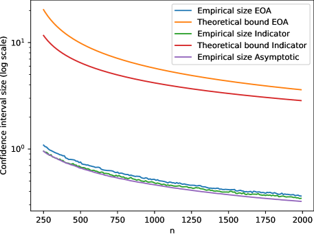
Figure 1: Comparison of the empirical sizes and the theoretical upper bounds on the sizes of the SPS-Indicator and SPS ellipsoidal outer approximation regions for $m=100$, $q=50$, $\delta=0.1$, $t_{0}=250$, $n=2000$ and $s=100$.

The difference between the empirical sizes of SPS-Indicator, SPS EOA and asymptotic confidence regions, furthermore, the theoretical bounds with confidence level $0.9$ ($\delta=0.1$) are shown in Fig. 1. We used quantiles for the empirical sizes in each iteration, i.e., the smallest number for which at least the specified portion $(s\cdot(1-\delta))$ of simulation realizations were below that number (from $s=100$ trials). The theoretical bounds were computed according to Theorems 2 and 3.

The results of this numerical experiment illustrate that our theoretical bounds capture well the empirical decrease rates of the confidence regions as well as the difference between these rates on the sizes of SPS-Indicator and SPS EOA confidence regions. The results also indicate that our theoretical bounds are a bit conservative. This, however, is an expected phenomenon, since these empirical regions are built (a posteriori) with data-driven algorithms, while the theoretical bounds are calculated (a priori) from concentration inequalities.

VI Conclusion

In this paper we have analyzed the sample complexity of data-driven confidence ellipsoids for linear regression problems which are constructed as outer approximations of the Sign-Perturbed Sums (SPS) confidence regions. These confidence ellipsoids share their centers (i.e., the least-squares estimate) and shape matrices (i.e., the empirical covariance of the regressors) with the classical asymptotic ellipsoids, only their radii are different. These radii can be calculated by convex programming methods resulting in distribution-free confidence ellipsoids with finite sample coverage guarantees.

Our results build upon the theory of concentration inequalities and give high probability upper bounds on the sizes of these confidence ellipsoids under the assumptions that the observation noises are independent, symmetric, nonatomic and subgaussian, as well as that the regressors are suitably exciting. We have also showed that the sizes shrink at the optimal rate.

Future research directions include extending our results to dynamical systems, e.g., to ARX and state-space models.

Appendix A Proof of Lemma 3

Proof.

The results of (59) and (61) will be combined to provide the claimed stochastic lower bound.

From (59), if $0\leq\varepsilon\leq 8\sigma^{2}d^{2}$, we have

$$\mathbb{P}\left(\frac{|X_{\scriptscriptstyle P}-\mathbb{E}X_{\scriptscriptstyle P}|}{n\lambda_{0}}\geq\varepsilon\right)\leq 2\exp\left(-\frac{\varepsilon^{2}n^{2}\lambda_{0}^{2}}{64d^{2}\sigma^{4}}\right),$$ (67)

which can be reformulated by introducing $\delta\doteq 4\exp(-\varepsilon^{2}n^{2}\lambda_{0}^{2}/(64d^{2}\sigma^{4}))$ as, for all $\delta:4\exp(-(nd\lambda_{0})^{2})\leq\delta\leq 2$, with probability (w.p.) at least $1-\delta/2$, it holds that

$$\frac{|X_{\scriptscriptstyle P}-\mathbb{E}X_{\scriptscriptstyle P}|}{n\lambda_{0}}\leq\frac{8d\sigma^{2}\ln^{\frac{1}{2}}(\tfrac{4}{\delta})}{n\lambda_{0}}.$$ (68)

Likewise, if $\varepsilon>8\sigma^{2}{d^{2}}$, for all $\delta$, such that $0\leq\delta<4\exp(-(nd\lambda_{0})^{2})$ we have, w.p. at least $1-\delta/2$, that

$$\frac{|X_{\scriptscriptstyle P}-\mathbb{E}X_{\scriptscriptstyle P}|}{n\lambda_{0}}\leq\frac{8\sigma^{2}\ln(\tfrac{4}{\delta})}{n\lambda_{0}}.$$ (69)

Combining these together we get, w.p. at least $1-\delta/2$, that

$$\frac{|X_{\scriptscriptstyle P}-\mathbb{E}X_{\scriptscriptstyle P}|}{n\lambda_{0}}\leq$$

$$\begin{cases}\dfrac{8d\sigma^{2}\ln^{\frac{1}{2}}(\tfrac{4}{\delta})}{n\lambda_{0}}\vspace{1mm}&4e^{-(nd\lambda_{0})^{2}}\leq\delta\leq 1,\\ \dfrac{8\sigma^{2}\ln(\tfrac{4}{\delta})}{n\lambda_{0}}&\delta<4e^{-(nd\lambda_{0})^{2}}.\end{cases}$$ (70)

In the proof of Lemma 1 [20, Appendix B] it is shown that a random variable in the form of $X=w_{n}^{\mathrm{T}}Mw_{n}$, where $M$ is a projection matrix with rank($M$)$=d$, can be upper bounded as $X\leq\sum_{i=1}^{d}\tilde{w}_{d,i}^{2}$, where $\{\tilde{w}_{d,i}\}$ are (zero mean) $\sigma$-subgaussians. Since $X_{\scriptscriptstyle P}$ is in this form, we have that

$$\mathbb{E}\big{[}X_{\scriptscriptstyle P}\big{]} \leq\mathbb{E}\left[\sum_{t=1}^{d}\tilde{w}_{d,i}^{2}\right]=\sum_{t=1}^{d}\mathbb{E}\left[\tilde{w}_{d,i}^{2}\right]=\sum_{t=1}^{d}\text{Var}\left[\tilde{w}_{d,i}\right]$$

$$\leq\sum_{t=1}^{d}\sigma^{2}=d\,\sigma^{2}.$$ (71)

Applying the reverse triangle inequality and that $\mathbb{E}X_{\scriptscriptstyle P}\leq d\sigma^{2}$:

$$\frac{|X_{\scriptscriptstyle P}-\mathbb{E}X_{\scriptscriptstyle P}|}{n\lambda_{0}}\geq\frac{|X_{\scriptscriptstyle P}|-|\mathbb{E}X_{\scriptscriptstyle P}|}{n\lambda_{0}}\geq\frac{|X_{\scriptscriptstyle P}|}{n\lambda_{0}}-\frac{d\sigma^{2}}{n\lambda_{0}},$$ (72)

and we have w.p. at least $1-\delta/2$ that

$$\frac{|X_{\scriptscriptstyle P}|}{n\lambda_{0}}\leq$$

$$\begin{cases}\dfrac{d\sigma^{2}\left(8\ln^{\frac{1}{2}}(\tfrac{4}{\delta})+1\right)}{n\lambda_{0}}\vspace{1mm}&4e^{-(nd\lambda_{0})^{2}}\leq\delta\leq 1,\\ \dfrac{\sigma^{2}\left(8\ln(\tfrac{4}{\delta})+d\right)}{n\lambda_{0}}&\delta<4e^{-(nd\lambda_{0})^{2}}.\end{cases}$$ (73)

Next, the concentration inequality result of (61) is reformulated as, w.p. at least $1-\delta/2$, we have

$$\frac{1+\lambda^{1/2}_{\text{max}}(K^{2})}{1-\lambda^{1/2}_{\text{max}}(K^{2})}\leq\frac{1+\left(\frac{2\kappa d^{2}\ln\left(\frac{4d}{\delta}\right)}{n^{\rho}}\right)^{\frac{1}{2}}}{1-\left(\frac{2\kappa d^{2}\ln\left(\frac{4d}{\delta}\right)}{n^{\rho}}\right)^{\frac{1}{2}}}$$

$$=\frac{n^{\frac{\rho}{2}}+\left(2\kappa d^{2}\ln\left(\frac{4d}{\delta}\right)\right)^{\frac{1}{2}}}{n^{\frac{\rho}{2}}-\left(2\kappa d^{2}\ln\left(\frac{4d}{\delta}\right)\right)^{\frac{1}{2}}}=\frac{n^{\frac{\rho}{2}}+g^{\frac{1}{2}}(\delta)}{n^{\frac{\rho}{2}}-g^{\frac{1}{2}}(\delta)},$$ (74)

where we used the definition of $g(\delta)$ (2). Using the union bound it can be shown that if

$$\mathbb{P}(Y_{1}\leq y_{1})\geq 1-p_{1}, \mathbb{P}(Y_{2}\leq y_{2})\geq 1-p_{2},$$ (75)

then

$$\mathbb{P}(Y_{1}Y_{2}\leq y_{1}y_{2})\geq 1-(p_{1}+p_{2}).$$ (76)

Combining the result of (75)-(76) with the stochastic lower bounds of (A) and (A) we conclude that w.p. at least $1-\delta$

$$\frac{|X_{\scriptscriptstyle P}|\left(1+\lambda^{1/2}_{\text{max}}(K^{2})\right)}{n\lambda_{0}\left(1-\lambda^{1/2}_{\text{max}}(K^{2})\right)}\leq$$

$$\begin{cases}\dfrac{d\sigma^{2}\left(8\ln^{\frac{1}{2}}(\tfrac{4}{\delta})+1\right)\left(n^{\frac{\rho}{2}}+g^{\frac{1}{2}}(\delta)\right)}{n\lambda_{0}\left(n^{\frac{\rho}{2}}-g^{\frac{1}{2}}(\delta)\right)}\vspace{1mm}&4e^{-(nd\lambda_{0})^{2}}\leq\delta\leq 1,\\ \dfrac{\sigma^{2}\left(8\ln(\tfrac{4}{\delta})+d\right)\left(n^{\frac{\rho}{2}}+g^{\frac{1}{2}}(\delta)\right)}{n\lambda_{0}\left(n^{\frac{\rho}{2}}-g^{\frac{1}{2}}(\delta)\right)}&\delta<4e^{-(nd\lambda_{0})^{2}}.\\ \end{cases}$$

The above stochastic lower bound can be applied to obtain a high probability upper bound for the size of the 0.5-level SPS EOA region. It is shown in (58), that for every $\theta\in\mathcal{O}_{0.5,n}$:

$$\|\theta-\hat{\theta}_{n}\|^{2}\leq\frac{\tfrac{1}{n}X_{\scriptscriptstyle P}(1+\lambda^{1/2}_{\text{max}}(K^{2}))}{\lambda_{0}(1-\lambda^{1/2}_{\text{max}}(K^{2}))},$$ (78)

consequently, it holds w.p. at least $1-\delta$ that

$$\sup_{\theta\in\mathcal{O}_{0.5,n}}\|\theta-\hat{\theta}_{n}\|\leq\dfrac{f(\delta)(n^{\frac{\rho}{2}}+g^{\frac{1}{2}}(\delta))^{\frac{1}{2}}}{\left(n\lambda_{0}(n^{\frac{\rho}{2}}-g^{\frac{1}{2}}(\delta))\right)^{\frac{1}{2}}},$$ (79)

where we used the definition of $f(\delta)$ from (2). ∎

Appendix B Technical Lemmas

Lemma 4.

Assuming A1 and that the SPS confidence region is bounded, it holds almost surely that

$$\|S_{1}(\hat{\theta}_{n})\|^{2}\neq 0.$$ (80)

Proof.

Using our notation (23)-(24) $S_{1}(\theta)$ can be written as

$$S_{1}(\theta)=\bar{R}_{n}^{-\frac{1}{2}}\frac{1}{n}\left(Q_{n}(\theta^{*}-\theta)+\Phi_{n}^{\mathrm{T}}D_{\alpha,n}w_{n}\right),$$ (81)

therefore

$$S_{1}(\hat{\theta}_{n}) =\frac{1}{n}\bar{R}_{n}^{-\frac{1}{2}}\left(Q_{n}(\theta^{*}-R_{n}^{-1}\Phi_{n}^{\mathrm{T}}y_{n})+\Phi_{n}^{\mathrm{T}}D_{\alpha,n}w_{n}\right)$$

$$=\frac{1}{n}\bar{R}_{n}^{-\frac{1}{2}}\left(Q_{n}(-R_{n}^{-1}\Phi_{n}^{\mathrm{T}}w_{n})+\Phi_{n}^{\mathrm{T}}D_{\alpha,n}w_{n}\right)$$

$$=\frac{1}{n}\bar{R}_{n}^{-\frac{1}{2}}\Phi_{n}^{\mathrm{T}}D_{\alpha,n}\left(I-\Phi_{n}R_{n}^{-1}\Phi_{n}^{\mathrm{T}}\right)w_{n}.$$ (82)

In [25] it is showed that if the confidence region is bounded, then $A$ is positive definite, consequently $\bar{R}_{n}^{-\frac{1}{2}}A\bar{R}_{n}^{-\frac{1}{2}}$ is also positive definite (A2), therefore it is full rank. Using our definition of $A$ (25), it can be written that $\bar{R}_{n}^{-\frac{1}{2}}A\bar{R}_{n}^{-\frac{1}{2}}=\bar{R}_{n}^{-\frac{1}{2}}\Phi^{\mathrm{T}}D_{\alpha,n}(I-\Phi_{n}R_{n}^{-1}\Phi_{n}^{\mathrm{T}})D_{\alpha,n}\Phi\bar{R}_{n}^{-\frac{1}{2}}$. Lets denote $L\doteq\bar{R}_{n}^{-\frac{1}{2}}\Phi^{\mathrm{T}}D_{\alpha,n}(I-\Phi_{n}R_{n}^{-1}\Phi_{n}^{\mathrm{T}})$. Since $L$ is a part of the product of the $d$-ranked matrix $\bar{R}_{n}^{-\frac{1}{2}}A\bar{R}_{n}^{-\frac{1}{2}}$, it follows that rank$(L)=d$. Notice that $S_{1}(\hat{\theta}_{n})=1/n\cdot Lw_{n}$, therefore by applying Lemma 6 we conclude that $S_{1}(\hat{\theta}_{n})\neq 0$ almost surely, hence $\|S_{1}(\hat{\theta}_{n})\|^{2}\neq 0$ almost surely. ∎

Lemma 5.

Assuming A1, A2 and $\lambda_{\text{max}}(K^{2})<1$, the following holds almost surely for $\xi=1/(1-\lambda_{\text{max}}(K^{2}))$,

$$\left(I-A^{\prime}_{0}(\xi)\left(A^{\prime}_{0}(\xi)\right)^{\dagger}\right)\xi b_{0}\neq 0,$$ (83)

where $A^{\prime}_{0}(\xi)$ and $b_{0}$ are defined in (29) and (21), respectively.

Proof.

Using the reformulation of $\xi A^{\prime}_{0}(\xi)$ from (39), we have

$$A^{\prime}_{0}(\xi) =V_{\Phi_{R}}U_{\Phi_{R}}^{\mathrm{T}}(-\tfrac{1}{\xi}I+I-K^{2})U_{\Phi_{R}}V_{\Phi_{R}}^{\mathrm{T}}$$

$$=V_{\Phi_{R}}U_{\Phi_{R}}^{\mathrm{T}}V_{K}(-\tfrac{1}{\xi}I+I-\Lambda_{K}^{2})V_{K}^{\mathrm{T}}U_{\Phi_{R}}V_{\Phi_{R}}^{\mathrm{T}},$$ (84)

where $K=V_{K}\Lambda_{K}V_{K}^{\mathrm{T}}$ is the eigendecomposition of $K$. Substituting $\xi=1/(1-\lambda_{\text{max}}(K^{2}))$ to the first part of (83) and using the decomposition above, we get

$$\left(I-A^{\prime}_{0}\left(\tfrac{1}{1-\lambda_{\text{max}}(K^{2})}\right)\left(A^{\prime}_{0}\left(\tfrac{1}{1-\lambda_{\text{max}}(K^{2})}\right)\right)^{\dagger}\right)=$$

$$V_{\Phi_{R}}U_{\Phi_{R}}^{\mathrm{T}}V_{K}D_{\text{max}}V_{K}^{\mathrm{T}}U_{\Phi_{R}}V_{\Phi_{R}}^{\mathrm{T}},$$ (85)

with $D_{\text{max}}\doteq\text{diag}(0,\dots,0,1,\dots,1)\in\mathbb{R}^{d\times d}$, where the number of ones equals to the multiplicity of $\lambda_{\text{max}}(K^{2})$ in $\Lambda_{K}^{2}$.

The vector $b_{0}$ defined in (21) can be rewritten by using the reformulation from (IV) as

$$b_{0} =\frac{1}{n^{\frac{1}{2}}}R_{n}^{-\frac{1}{2}}Q_{n}R_{n}^{-1}BD_{\alpha,n}y_{n}$$

$$=\frac{1}{n^{\frac{1}{2}}}R_{n}^{-\frac{1}{2}}Q_{n}R_{n}^{-1}BD_{\alpha,n}w_{n}.$$ (86)

Let

$$B_{0}\doteq R_{n}^{-\frac{1}{2}}Q_{n}R_{n}^{-1}BD_{\alpha,n}.$$ (87)

Notice that $BB^{\mathrm{T}}=A$, since

$$BB^{\mathrm{T}}=\left(\Phi_{n}^{\mathrm{T}}-Q_{n}R_{n}^{-1}\Phi_{n}^{\mathrm{T}}D_{\alpha,n}\right)\left(\Phi_{n}-D_{\alpha,n}\Phi_{n}R_{n}^{-1}Q_{n}\right)=$$

$$\left(R_{n}-Q_{n}R_{n}^{-1}Q_{n}-Q_{n}R_{n}^{-1}Q_{n}+Q_{n}R_{n}^{-1}Q_{n}\right)=A.$$ (88)

Then, it holds that

$$B_{0}B_{0}^{\mathrm{T}} =R_{n}^{-\frac{1}{2}}Q_{n}R_{n}^{-1}BD_{\alpha,n}D_{\alpha,n}B^{\mathrm{T}}R_{n}^{-1}Q_{n}R_{n}^{-\frac{1}{2}}$$

$$=R_{n}^{-\frac{1}{2}}Q_{n}R_{n}^{-1}AR_{n}^{-1}Q_{n}R_{n}^{-\frac{1}{2}}.$$ (89)

Using the same reformulations as in (IV)-(IV), specifically $A=\Phi_{R,n}^{\mathrm{T}}(I-K^{2})\Phi_{R,n}$, $R^{-1}=\Phi_{R,n}^{-1}\Phi_{R,n}^{-\mathrm{T}}$ and $Q_{n}=\Phi_{R,n}^{\mathrm{T}}K\Phi_{R,n}$ it can be written that

$$Q_{n}R_{n}^{-1}AR_{n}^{-1}Q_{n}=\Phi_{R,n}^{\mathrm{T}}K(I-K^{2})K\Phi_{R,n}.$$ (90)

Writing back (90) to (B) and applying $R_{n}^{-1/2}=V_{\Phi_{R}}\Sigma_{\Phi_{R}}^{-1}V_{\Phi_{R}}^{\mathrm{T}}$ and $\Phi_{R,n}=U_{\Phi_{R}}\Sigma_{\Phi_{R}}V_{\Phi_{R}}^{\mathrm{T}}$ from (38), we get

$$B_{0}B_{0}^{\mathrm{T}}=V_{\Phi_{R}}U_{\Phi_{R}}^{\mathrm{T}}K(I-K^{2})KU_{\Phi_{R}}V_{\Phi_{R}}^{\mathrm{T}}.$$ (91)

Finally, using again the eigendecomposition of $K$

$$B_{0}B_{0}^{\mathrm{T}}=V_{\Phi_{R}}U_{\Phi_{R}}^{\mathrm{T}}V_{K}\Lambda_{K}(I-\Lambda_{K}^{2})\Lambda_{K}V_{K}^{\mathrm{T}}U_{\Phi_{R}}V_{\Phi_{R}}^{\mathrm{T}}.$$ (92)

Notice the similarity between (B) and (92). In these formulas $-\tfrac{1}{\xi}I+I-\Lambda_{K}^{2}$ and $\Lambda_{K}(I-\Lambda_{K}^{2})\Lambda_{K}$ are diagonal and $V_{\Phi_{R}}U_{\Phi_{R}}^{\mathrm{T}}V_{K}$ is orthonormal, since $V_{K}^{\mathrm{T}}U_{\Phi_{R}}V_{\Phi_{R}}^{\mathrm{T}}V_{\Phi_{R}}U_{\Phi_{R}}^{\mathrm{T}}V_{K}=I$. It follows that (B) and (92) are eigendecompositions of $A^{\prime}_{0}(\xi)$ and $B_{0}B_{0}^{\mathrm{T}}$, therefore they can be written as $A^{\prime}_{0}(\xi)=V_{A_{0}}(-\tfrac{1}{\xi}I+I-\Lambda_{K}^{2})V_{A_{0}}^{\mathrm{T}}$ and $B_{0}B_{0}^{\mathrm{T}}=V_{A_{0}}\Lambda_{K}(I-\Lambda_{K}^{2})\Lambda_{K}V_{A_{0}}^{\mathrm{T}}$, where we used the same arrangements of eigenvalues and eigenvectors. Using the SVD decomposition of $B_{0}=U_{B_{0}}\Sigma_{B_{0}}V_{B_{0}}^{\mathrm{T}}$ and the above eigendecomposition $B_{0}B_{0}^{\mathrm{T}}=V_{A_{0}}\Lambda_{K}(I-\Lambda_{K}^{2})\Lambda_{K}V_{A_{0}}^{\mathrm{T}}$ it holds that

$$U_{B_{0}}\Sigma_{B_{0}}^{2}U_{B_{0}}^{\mathrm{T}}=V_{A_{0}}\Lambda_{K}(I-\Lambda_{K}^{2})\Lambda_{K}V_{A_{0}}^{\mathrm{T}}.$$ (93)

From equation (93), it follows that there is an arrangement of eigenvalues in $\Sigma_{B_{0}}^{2}$ and $\Lambda_{K}(I-\Lambda_{K}^{2})\Lambda_{K}$ that for their corresponding eigenvectors $U_{B_{0}}=V_{A_{0}}$. Using this arrangement of eigenvectors and eigenvalues, i.e., $U_{B_{0}}=V_{A_{0}}$ and $\Sigma_{B_{0}}=((I-\Lambda_{K}^{2})\Lambda_{K}^{2})^{1/2}$, furthermore our result from (B), we conclude that in case $\xi=1/(1-\lambda_{\text{max}}(K^{2}))$, we have

$$\left(I-A^{\prime}_{0}(\xi)\left(A^{\prime}_{0}(\xi)\right)^{\dagger}\right)\xi b_{0}=$$

$$\frac{1}{1-\lambda_{\text{max}}(K^{2})}V_{A_{0}}D_{\text{max}}V_{A_{0}}^{\mathrm{T}}B_{0}w_{n}=$$

$$\frac{1}{n^{\frac{1}{2}}(1-\lambda_{\text{max}}(K^{2}))}V_{A_{0}}D_{\text{max}}V_{A_{0}}^{\mathrm{T}}U_{B_{0}}\Sigma_{B_{0}}V_{B_{0}}^{\mathrm{T}}w_{n}=$$

$$\frac{1}{n^{\frac{1}{2}}(1-\lambda_{\text{max}}(K^{2}))}U_{B_{0}}D_{\text{max}}((I-\Lambda_{K}^{2})\Lambda_{K}^{2})^{\frac{1}{2}}V_{B_{0}}^{\mathrm{T}}w_{n}=$$

$$\frac{\max_{i}\left\lvert\lambda_{i}(K)\right\rvert}{(n(1-\lambda_{\text{max}}(K^{2})))^{\frac{1}{2}}}U_{B_{0}}D_{\text{max}}V_{B_{0}}^{\mathrm{T}}w_{n},$$ (94)

where in the last step we used that $D_{\text{max}}$ “selects” the largest eigenvalues in the ordering, as in (B), which equals $\max_{i}\left\lvert\lambda_{i}(K)\right\rvert\cdot(1-\lambda_{\text{max}}(K^{2}))^{1/2}$. It was shown in the proof of Theorem 3 that the eigenvalues of matrix $K$ satisfy $\forall i:0<\left\lvert\lambda_{i}(K)\right\rvert\leq 1$ and we assume that $\lambda_{\text{max}}(K^{2})<1$, therefore $(\max\left\lvert\lambda_{i}(K)\right\rvert)/((n(1-\lambda_{\text{max}}(K^{2})))^{1/2})\neq 0$. It holds that $1\leq\text{rank}(U_{B_{0}}D_{\text{max}}V_{B_{0}}^{\mathrm{T}})\leq d$, which follows from the fact that the number of ones in $D_{\text{max}}$ equals to the multiplicity of $\lambda_{\text{max}}(K^{2})$ in $\Lambda_{K}^{2}$. Then, $U_{B_{0}}D_{\text{max}}V_{B_{0}}^{\mathrm{T}}w_{n}$ is almost surely nonzero, as $w_{n}$ consist of independent, nonatomic random variables (A1), therefore Lemma 6 can be applied. ∎

Lemma 6.

Let $M\in\mathbb{R}^{k\times n}$ with $\text{rank}(M)>0$ and $w_{0}\in\mathbb{R}^{n}$ a vector of independent nonatomic random variables. Then,

$$\mathbb{P}(Mw_{0}\neq 0)=1.$$ (95)

Proof.

Since $\text{rank}(M)>0$, there is at least one row of $M$ which is nonzero. Let $\vec{m}$ denote any of these row vectors. Observe that if it enough to prove that $\vec{m}w_{0}\neq 0$ almost surely. There exists an index $i$ with $\vec{m}_{i}\neq 0$. Then, we have

$$\vec{m}w_{0} =\sum_{t=1}^{n}\vec{m}_{t}W_{0,t}=\vec{m}_{i}\left(W_{0,i}+\sum_{\begin{subarray}{c}t=1,t\neq i\end{subarray}}^{n}\frac{\vec{m}_{t}}{\vec{m}_{i}}W_{0,t}\right)$$

$$=\vec{m}_{i}\left(W_{0,i}+\sum_{\begin{subarray}{c}t=1,t\neq i\end{subarray}}^{n}\vec{m}^{\prime}_{t}W_{0,t}\right),$$ (96)

where $w_{0}=[W_{0,1},W_{0,2},\dots,W_{0,n}]^{\mathrm{T}}$. $Mw_{0}=0$, if $W_{0,i}+\sum_{\begin{subarray}{c}t=1,t\neq i\end{subarray}}^{n}\vec{m}^{\prime}_{t}W_{0,t}=0$, hence we investigate the probability $\mathbb{P}\left(W_{0,i}+\sum_{\begin{subarray}{c}t=1,t\neq i\end{subarray}}^{n}\vec{m}^{\prime}_{t}W_{0,t}=0\right)$. Using the law of total expectation it can be derived that

$$\mathbb{P}\left(W_{0,i}+\sum_{\begin{subarray}{c}t=1,t\neq i\end{subarray}}^{n}\vec{m}^{\prime}_{t}W_{0,t}=0\right)=$$ (97)

$$\mathbb{E}\left[\mathbb{P}\left(W_{0,i}+\sum_{\begin{subarray}{c}t=1,t\neq i\end{subarray}}^{n}\vec{m}^{\prime}_{t}W_{0,t}=0\Bigg{|}\{W_{0,t}\}_{\begin{subarray}{c}t=1,t\neq i\end{subarray}}^{n}\right)\right]=0,$$

since $W_{0,i}$ is nonatomic for every $i$. ∎

Lemma 7.

Let $P(\xi)$ be defined as in (IV), that is

$$P(\xi)\,=\; D_{\alpha,n}B^{\mathrm{T}}\Big{[}R_{n}^{-1}Q_{n}R_{n}^{-\frac{1}{2}}\left(A^{\prime}_{0}(\xi)\right)^{\dagger}R_{n}^{-\frac{1}{2}}Q_{n}R_{n}^{-1}$$

$$+R_{n}^{-1}\Big{]}BD_{\alpha,n}.$$ (98)

Assume A2, $\forall\,i:0<\left\lvert\lambda_{i}(K)\right\rvert<1$ and $\xi>1/(1-\lambda_{\text{max}}(K^{2}))$. Then, $P(\xi)$ is positive semidefinite and $\text{rank}(P(\xi))=d$, furthermore for every nonzero eigenvalue of $P(\xi)$,

$$\lambda_{i}(P(\xi))=\frac{\xi\lambda_{i}^{2}(K)-\xi-\lambda_{i}^{2}(K)+1}{\xi\lambda_{i}^{2}(K)-\xi+1},$$ (99)

where $K$ is defined in (35). Note that $\lambda_{i}(\cdot)$ are ordered, that is $\lambda_{1}(\cdot)\geq\lambda_{2}(\cdot)\geq\cdots\geq\lambda_{d}(\cdot)$.

Proof.

Lets denote the middle part of the product given in the definition of $P(\xi)$ (7) as

$$P_{1}(\xi)\doteq R_{n}^{-1}Q_{n}R_{n}^{-\frac{1}{2}}\left(A^{\prime}_{0}(\xi)\right)^{\dagger}R_{n}^{-\frac{1}{2}}Q_{n}R_{n}^{-1}+R_{n}^{-1}.$$ (100)

Using the same reformulations as in (IV)-(IV), namely $R^{-1}=\Phi_{R,n}^{-1}\Phi_{R,n}^{-\mathrm{T}}$, $Q_{n}=\Phi_{R,n}^{\mathrm{T}}K\Phi_{R,n}$, $R_{n}^{-1/2}=V_{\Phi_{R}}\Sigma_{\Phi_{R}}^{-1}V_{\Phi_{R}}^{\mathrm{T}}$ and $\Phi_{R,n}=U_{\Phi_{R}}\Sigma_{\Phi_{R}}V_{\Phi_{R}}^{\mathrm{T}}$, we have

$$P_{1}(\xi) =\Phi_{R,n}^{-1}\Big{(}K\Phi_{R,n}R_{n}^{-\frac{1}{2}}\left(A^{\prime}_{0}(\xi)\right)^{\dagger}R_{n}^{-\frac{1}{2}}\Phi_{R,n}K+I\Big{)}\Phi_{R,n}^{\mathrm{-T}}$$

$$=\Phi_{R,n}^{-1}\Big{(}KU_{\Phi_{R}}V_{\Phi_{R}}^{\mathrm{T}}\left(A^{\prime}_{0}(\xi)\right)^{\dagger}V_{\Phi_{R}}U_{\Phi_{R}}^{\mathrm{T}}K+I\Big{)}\Phi_{R,n}^{\mathrm{-T}}.$$ (101)

The matrix $A^{\prime}_{0}(\xi)$ can be written as in (39)

$$A^{\prime}_{0}(\xi)=V_{\Phi_{R}}U_{\Phi_{R}}^{\mathrm{T}}(-\tfrac{1}{\xi}I+I-K^{2})U_{\Phi_{R}}V_{\Phi_{R}}^{\mathrm{T}},$$ (102)

therefore,

$$P_{1}(\xi)=\Phi_{R,n}^{-1}\left(K\left(-\tfrac{1}{\xi}I+I-K^{2}\right)^{\dagger}K+I\right)\Phi_{R,n}^{\mathrm{-T}}.$$ (103)

Using the eigendecomposition of $K=V_{K}\Lambda_{K}V_{K}^{\mathrm{T}}$ it holds that

$$P_{1}(\xi) =\Phi_{R,n}^{-1}V_{K}\left(\Lambda_{K}\left(I-\Lambda_{K}^{2}-\tfrac{1}{\xi}I\right)^{\dagger}\Lambda_{K}+I\right)V_{K}^{\mathrm{T}}\Phi_{R,n}^{\mathrm{-T}}$$

$$=\Phi_{R,n}^{-1}V_{K}\Lambda^{\prime}_{K}(\xi)V_{K}^{\mathrm{T}}\Phi_{R,n}^{\mathrm{-T}},$$ (104)

where

$$\Lambda^{\prime}_{K}(\xi)\doteq\Lambda_{K}\left(I-\Lambda_{K}^{2}-\tfrac{1}{\xi}I\right)^{\dagger}\Lambda_{K}+I.$$ (105)

Notice that as we assume $\xi>1/(1-\lambda_{\text{max}}(K^{2}))$, it holds for every diagonal element (eigenvalue) of $(I-\Lambda_{K}^{2}-{I}/{\xi})$ that

$$1-\lambda_{i}(K^{2})-\frac{1}{\xi} >1-\lambda_{i}(K^{2})-(1-\lambda_{\text{max}}(K^{2}))$$

$$=\lambda_{\text{max}}(K^{2})-\lambda_{i}(K^{2})\geq 0,$$ (106)

therefore $(I-\Lambda_{K}^{2}-{I}/{\xi})$ is positive definite. Since we assume that $\forall\,i:0<\left\lvert\lambda_{i}(K)\right\rvert<1$, it follows that $\Lambda^{\prime}_{K}(\xi)$ is also positive definite. Substituting our reformulation of $P_{1}(\xi)$ from (B) back to $P(\xi)$ (7), we get

$$P(\xi)=D_{\alpha,n}B^{\mathrm{T}}\Phi_{R,n}^{-1}V_{K}\Lambda^{\prime}_{K}(\xi)V_{K}^{\mathrm{T}}\Phi_{R,n}^{\mathrm{-T}}BD_{\alpha,n}.$$ (107)

By introducing $E\doteq\Phi_{R,n}^{\mathrm{-T}}BD_{\alpha,n}$, recalling that $BB^{\mathrm{T}}=A$ (B) and using the reformulation of $A$ from (IV)-(IV) with the eigendecomposition of $K$, it can be derived that

$$EE^{\mathrm{T}} =\Phi_{R,n}^{\mathrm{-T}}BD_{\alpha,n}D_{\alpha,n}B^{\mathrm{T}}\Phi_{R,n}^{-1}=\Phi_{R,n}^{\mathrm{-T}}A\Phi_{R,n}^{-1}$$

$$=I-K^{2}=V_{K}(I-\Lambda_{K}^{2})V_{K}^{\mathrm{T}}.$$ (108)

It follows that the full SVD decomposition of $E$ is

$$E=\Phi_{R,n}^{\mathrm{-T}}BD_{\alpha,n}=V_{K}\big{[}(I-\Lambda_{K}^{2})^{1/2}\quad 0\big{]}V_{E}^{\mathrm{T}},$$ (109)

where in (B) and (109) we used the same arrangement of singular and eigenvalues. Substituting (109) back to (107) we get the eigendecomposition of $P(\xi)$ as

$$P(\xi)= V_{E}\big{[}(I-\Lambda_{K}^{2})^{1/2}\quad 0\big{]}^{\mathrm{T}}\Lambda^{\prime}_{K}(\xi)$$

$$\cdot\big{[}(I-\Lambda_{K}^{2})^{1/2}\quad 0\big{]}V_{E}^{\mathrm{T}},$$ (110)

since $V_{E}$ is orthonormal and $[(I-\Lambda_{K}^{2})^{1/2}\quad 0\big{]}^{\mathrm{T}}\Lambda^{\prime}_{K}(\xi)[(I-\Lambda_{K}^{2})^{1/2}\quad 0\big{]}$ is diagonal. Recall that $\Lambda^{\prime}_{K}(\xi)$ is positive definite and that we assume $\forall\,i:0<\left\lvert\lambda_{i}(K)\right\rvert<1$, therefore $P(\xi)$ has exactly $d$ positive eigenvalues, hence $\text{rank}(P(\xi))=d$. Then, the nonzero eigenvalues of $P(\xi)$ are given as

$$\lambda_{i}(P(\xi)) =\left(\tfrac{\lambda_{i}^{2}(K)}{1-\lambda_{i}^{2}(K)-\tfrac{1}{\xi}}+1\right)(1-\lambda_{i}^{2}(K))$$

$$=\frac{\xi\lambda_{i}^{2}(K)-\xi-\lambda_{i}^{2}(K)+1}{\xi\lambda_{i}^{2}(K)-\xi+1},$$ (111)

where we used (105) and that $\Lambda^{\prime}_{K}(\xi)$ is invertible. ∎

References

- [1] L. Ljung, System Identification: Theory for the User, 2nd ed. Prentice Hall, Upper Saddle River, 1999.
- [2] A. Carè, B. Cs. Csáji, M. Campi, and E. Weyer, “Finite-sample system identification: An overview and a new correlation method,” IEEE Control Systems Letters, vol. 2, no. 1, pp. 61 – 66, 2018.
- [3] M. Simchowitz, H. Mania, S. Tu, M. I. Jordan, and B. Recht, “Learning without mixing: Towards a sharp analysis of linear system identification,” in 31st Conference On Learning Theory (COLT), Stockholm, Sweden, 2018, pp. 439–473.
- [4] S. Oymak and N. Ozay, “Revisiting Ho–Kalman-based system identification: Robustness and finite-sample analysis,” IEEE Transactions on Automatic Control, vol. 67, no. 4, pp. 1914–1928, 2021.
- [5] S. Basu, X. Li, and G. Michailidis, “Low rank and structured modeling of high-dimensional vector autoregressions,” IEEE Transactions on Signal Processing, vol. 67, no. 5, pp. 1207–1222, 2019.
- [6] B. Djehiche, O. Mazhar, and C. R. Rojas, “Finite impulse response models: A non-asymptotic analysis of the least squares estimator,” Bernoulli, vol. 27, no. 2, pp. 976 – 1000, 2021.
- [7] Y. Yi and M. Neykov, “Non-asymptotic bounds for the estimator in linear regression with uniform noise,” Bernoulli, vol. 30, no. 1, pp. 534 – 553, 2024.
- [8] M. Milanese, J. Norton, H. Piet-Lahanier, and É. Walter, Bounding Approaches to System Identification. Springer, 2013.
- [9] M. Casini, A. Garulli, and A. Vicino, “Input design in worst-case system identification with quantized measurements,” Automatica, vol. 48, no. 12, pp. 2997–3007, 2012.
- [10] ——, “Input design in worst-case system identification using binary sensors,” IEEE Transactions on Automatic Control, vol. 56, pp. 1186–1991, 2011.
- [11] M. Lauricella and L. Fagiano, “Set membership identification of linear systems with guaranteed simulation accuracy,” IEEE Transactions on Automatic Control, vol. 65, no. 12, pp. 5189–5204, 2020.
- [12] A. Tsiamis, I. Ziemann, N. Matni, and G. J. Pappas, “Statistical learning theory for control: A finite-sample perspective,” IEEE Control Systems Magazine, vol. 43, no. 6, pp. 67–97, 2023.
- [13] M. C. Campi and E. Weyer, “Guaranteed non-asymptotic confidence regions in system identification,” Automatica, pp. 1751–1764, 2005.
- [14] B. Cs. Csáji, M. C. Campi, and E. Weyer, “Sign-Perturbed Sums: A new system identification approach for constructing exact non-asymptotic confidence regions in linear regression models,” IEEE Transactions on Signal Processing, vol. 63, no. 1, pp. 169–181, 2015.
- [15] C.-Y. Han, M. Kieffer, and A. Lambert, “Guaranteed confidence region characterization for source localization using rss measurements,” Signal Processing, vol. 152, pp. 104–117, 2018.
- [16] V. Zambianchi, F. Bassi, A. Calisti, D. Dardari, M. Kieffer, and G. Pasolini, “Distributed nonasymptotic confidence region computation over sensor networks,” IEEE Transactions on Signal and Information Processing over Networks, vol. 4, no. 2, pp. 308–324, 2018.
- [17] B. Cs. Csáji, M. C. Campi, and E. Weyer, “Sign-Perturbed Sums (SPS): A method for constructing exact finite-sample confidence regions for general linear systems,” in 51st IEEE Conference on Decision and Control, Maui, Hawaii, 2012, pp. 7321–7326.
- [18] Sz. Szentpéteri and B. Cs. Csáji, “Non-asymptotic state-space identification of closed-loop stochastic linear systems using instrumental variables,” Systems and Control Letters, vol. 178, p. 105565, 2023.
- [19] E. Weyer, M. C. Campi, and B. Cs. Csáji, “Asymptotic properties of SPS confidence regions,” Automatica, vol. 81, pp. 287–294, 2017.
- [20] Sz. Szentpéteri and B. Cs. Csáji, “Sample complexity of the Sign-Perturbed Sums method,” Automatica, 2024 (accepted, to be published). [Online]. Available: https://arxiv.org/pdf/2409.01243
- [21] V. Volpe, B. Cs. Csáji, A. Carè, E. Weyer, and M. C. Campi, “Sign-Perturbed Sums (SPS) with instrumental variables for the identification of ARX systems,” in 54th IEEE Conference on Decision and Control (CDC), Osaka, Japan, 2015, pp. 2115–2120.
- [22] M. J. Wainwright, High-Dimensional Statistics: A Non-Asymptotic Viewpoint. Cambridge University Press, 2019.
- [23] E. J. Candès and B. Recht, “Exact matrix completion via convex optimization,” Foundations of Computational Mathematics, vol. 9, pp. 717–772, 2008.
- [24] Sz. Szentpéteri and B. Cs. Csáji, “Sample complexity of the Sign-Perturbed Sums identification method: Scalar case,” in 22nd IFAC (International Federation of Automatic Control) World Congress, Yokohama, Japan, 2023, pp. 11 123–11 130.
- [25] A. Carè, “A simple condition for the boundedness of Sign-Perturbed-Sums (SPS) confidence regions,” Automatica, vol. 139, p. 110150, 2022.
- [26] S. Boyd and L. Vandenberghe, Convex Optimization. Cambridge University Press, 2009.