Double Index Calculus Algorithm: Faster Solving Discrete Logarithm Problem in Finite Prime Field
Abstract
Solving the discrete logarithm problem in a finite prime field is an extremely important computing problem in modern cryptography. The hardness of solving the discrete logarithm problem in a finite prime field is the security foundation of numerous cryptography schemes. In this paper, we propose the double index calculus algorithm to solve the discrete logarithm problem in a finite prime field. Our algorithm is faster than the index calculus algorithm, which is the state-of-the-art algorithm for solving the discrete logarithm problem in a finite prime field. Empirical experiment results indicate that our algorithm could be more than a 30-fold increase in computing speed than the index calculus algorithm when the bit length of the order of prime field is 70 bits. In addition, our algorithm is more general than the index calculus algorithm. Specifically, when the base of the target discrete logarithm problem is not the multiplication generator, the index calculus algorithm may fail to solve the discrete logarithm problem while our algorithm still can work.
Index Terms:
Discrete logarithm problem, Index calculus algorithm, Finite prime field.I Introduction
The discrete logarithm problem in a finite prime field is an important computing problem in modern cryptography. In 1976, Diffie and Hellman built the first key exchange protocol on the discrete logarithm problem [1]. After that, massive cryptography schemes based their security on the hardness of solving the discrete logarithm problem in a finite prime field such as public-key encryption schemes [2, 3], digital signature schemes [4], deniable authenticated encryption schemes [5], and so on.
Several algorithms have been proposed to solve the discrete logarithm problem, including the baby-step giant-step algorithm [6], the PohligHellman algorithm [7], the rho together with kangaroo algorithm [8], and index calculus algorithm (which first appeared in [9, 10, 11], and which was rediscovered and analyzed by [12, 13, 8]). The index calculus algorithm is the state-of-the-art algorithm to solve the discrete logarithm problem in the finite prime field [14, 15].
The index calculus algorithm comprises two phases. In the first phase, discrete logarithms of all primes in factor base (which consists of all primes smaller than a bound named smoothness bound) are calculated. Specifically, assume that the target discrete logarithm problem is to find such that , where is a large prime (the order of finite prime field) and is the multiplication generator of field. Discrete logarithms of all primes in factor base are calculated by the equations system (2). To construct the equations system (2), massive integers are randomly generated to find integers such that
| (1) |
where are all primes in factor base and also are all primes smaller than smoothness bound. The integer satisfying the equation (1) is named smooth integer. For example, is -smooth.
| (2) |
Here, represents the discrete logarithm of prime base modulo . In the second phase, the discrete logarithm of the given integer is calculated by finding another random integer such that . Specifically, the target discrete logarithm is calculated by the following equation (3), namely
| (3) | |||||
Continuous efforts are dedicated to improving the index calculus algorithm and many variants of index calculus algorithm are proposed. The number field sieve [16] and the function field sieve [17] are famous variants of the index calculus algorithm and they are both sub-exponential time algorithms for solving the discrete logarithm problem in a finite prime field. Sieve methods improve the index calculus algorithm a lot because sieve methods can find random integers , , , , mentioned above much faster. In brief, the all famous successful variants of index calculus algorithm achieve faster solving discrete logarithm problem by constructing methods to find , , , , mentioned above faster.
In this paper, we speed up solving the discrete logarithm problem in a different and challenging way: reduce the number of discrete logarithms which must be obtained before the target discrete logarithm problem could be solved. In particular, to solve the target discrete logarithm problem, index calculus algorithm together with its all famous successful variants has to calculated discrete logarithms (namely, , , , , ), where is the number of primes in factor base. We construct an algorithm which can solve the target discrete logarithm problem, and the number of discrete logarithms our algorithm needs to obtain before solving the target discrete logarithm problem could be less than . Due to the decrease in the number of discrete logarithms that need to be obtained before solving the target discrete logarithm, our algorithm can solve the discrete logarithm problem much faster.
I-A Our Contribution
We make a theoretical breakthrough. Specifically, in the index calculus algorithm as well as its all variants, the target discrete logarithm problem can be successfully solved under the condition that at least discrete logarithms have to be found together. Here, is the number of primes in factor base. However, the double index calculus algorithm proposed in this paper could solve the target discrete logarithm problem when the number of discrete logarithms obtained is less than . Due to the decrease in the number of discrete logarithms that have to be obtained, calculation speed of our algorithm increase a lot.
I-B Advantages of Our Algorithm
Our algorithm has three advantages, namely fast calculation speed, high generality, and compatibility with tricks which other variants of index calculus algorithm utilize to speed up finding smooth integers (namely, integers satisfying equation (1)).
First, our algorithm outperforms the state-of-the-art index calculus algorithm significantly in computing speed when solving the discrete logarithm problem in a finite prime field. We compare our algorithm with the index calculus algorithm theoretically in TABLE II and prove that our algorithm is faster. Through empirical experiments, we observe that our algorithm achieves a speed advantage exceeding 30 times (75426/221134, these data are referenced in TABLE IV ) in some cases over the fastest index calculus algorithm when the bit length of the order of prime field is relatively large 70 bits. Empirical experiment results also imply that our algorithm may be faster than the fastest index calculus algorithm more than 30 times as the bit length continues to increase from 70 bits.
Our algorithm is more general than the index calculus algorithm. Specifically, when the base of the discrete logarithm problem is not the multiplication generator of the finite prime field, the discrete logarithms of some primes in factor base may not exist, which may cause the index calculus algorithm to fail. However, our algorithm still can work even if the discrete logarithms of some primes do not exist. Thus, our algorithm is more general in terms of whether or not the base of the discrete logarithm problem needs to be a multiplication generator.
Our algorithm also can utilize tricks of speeding up finding smooth integers to speed up solving the discrete logarithm problem further. In particular, our algorithm can utilize all tricks (which speed up solving the discrete logarithm problem by speeding up finding smooth integer first) of other variants of index calculus algorithm to find smooth integers first. And then, the tricks constructed in this paper can be utilized to reduce the number of needed smooth integers further. This advantage makes our algorithm faster than the index calculus algorithm together with its all famous variants.
I-C Technical Overview
New way solving discrete logarithm problem. Each different algorithm to solve the discrete logarithm problem builds its own unique equation related to the target discrete logarithm problem and the target discrete logarithm is obtained by the build equation. For example, the index calculus algorithm utilizes the equation (4), namely
| (4) | |||||
to calculate the target discrete logarithm after the discrete logarithms of all primes in factor base are obtained. In the baby step giant step algorithm, the target discrete logarithm is obtained by fining , , and such that
| (5) |
when the target discrete logarithm problem is to find such that . In this paper, we utilize a new equations system to calculate the target discrete logarithm. Specifically, find , , and such that
| (6) |
The target discrete logarithm is calculated by the equation (7)
| (7) |
The way finding needed integers. The key to success of our algorithm is to find , , and in the equations system (6). Instead of fixing first, we build two equations systems to calculate discrete logarithms base and , respectively. And then, identify the integer whose discrete logarithms base and base are both obtained. In particular, a series of random integers is generated to find such that , where , , , are primes in factor base. By solving equations system
| (8) |
discrete logarithms of some primes could be obtained although not discrete logarithms of all primes in factor base are obtained when is less than the number of primes in factor base. Similarly, by building the equations system
| (9) |
discrete logarithms of some primes base could be obtained although not discrete logarithms of all primes in factor base are obtained. By comparing solutions of two equations systems, the prime whose discrete logarithms base and are both obtained can be identified.
Decrease the number of discrete logarithms needed. The key to speed up solving the target discrete logarithm problem is to reduce the total number of needed discrete logarithms to solve the target discrete logarithm. To solve the target discrete logarithm problem, the index calculus algorithm has to obtain discrete logarithms of primes in factor base. Our algorithm can solve the target discrete logarithm problem through less than discrete logarithms of primes in factor base.
In particular, the index calculus algorithm has to obtain discrete logarithms of all primes in factor base before it solves the target discrete logarithm problem. Thus, index calculus algorithm must calculate discrete logarithms in total. Our algorithm can solve the target discrete logarithm problem when discrete logarithms of some primes not all primes in factor base are obtained. For example, as long as and are both obtained the target discrete logarithm problem can be solved. In this extremely nice case, only two discrete logarithms are needed to solve the target discrete logarithm problem through our algorithm.
In our algorithm, one nice case happens with an extremely small probability but the number of nice cases is extremely massive, resulting in that the total probability that nice cases happen is large. Here, the nice case is the case where the target discrete logarithm can be obtained through less than discrete logarithms of primes in factor base. is the number of primes in factor base. Specifically, when only one prime’s two discrete logarithms are calculated through the equations systems (8) and (9) respectively, the number of nice cases is . These cases are . When two primes’ discrete logarithms are calculated through the equations systems (8) and (9) respectively, the number of nice cases is . These cases are , , , . Roughly speaking, the number of nice cases are
| (10) |
where is the number of primes in factor base. The number represented by formula (10) is an extremely massive number, resulting in that nice cases happen with a large probability in total although each nice case happens with a small probability. In other words, our algorithm can solve the target discrete logarithm problem with a big probability through calculating less than discrete logarithms of primes in factor. That is, our algorithm can solve the discrete logarithm problem faster than index calculus algorithm which is the fastest algorithm to solve the discrete logarithm problem.
II Preliminaries
In this section, preliminaries are introduced, including the definition of discrete logarithm problem and the concept of smooth integer. At the last, the notations used in this paper are summarized in a table.
II-A Discrete Logarithm Problem
The discrete logarithm problem in the finite prime field holds significant importance in modern cryptography. Numerous cryptographic schemes rely on the assumption that solving the discrete logarithm problem in the finite prime field is computationally difficult. The definition of the discrete logarithm problem is as follows:
Discrete logarithm problem: In a finite prime field with elements, for given integers and , find the smallest non-negative integer such that , where usually is a large prime integer.
II-B smooth Integer
The smooth integer is an important concept in cryptography and it relies on factorization of integers. The definition of smooth integer is as follows:
B-smooth integer: An integer is -smooth if its all prime factors are less than or equal to .
For example, 77=7*11 is an 11-smooth integer. Main notations used in this paper are summarized in TABLE I.
| notations | description |
| multiplication generator of filed | |
| target discrete logarithm | |
| large prime integer | |
| discrete logarithm of base modulo a large prime integer | |
| smoothness bound | |
| -smooth | an integer is -smooth if its all prime factors are smaller than or equal to |
| factor base | |
| k | the number of primes in factor base |
| intersection of and | |
| the number of elements in a list or a set | |
| probability |
III Double Index Calculus Algorithm
In this section, we begin by elaborating on our idea, followed by a formal presentation of our algorithm. At last, we verify the correctness of our algorithm and compare our algorithm with the state-of-the-art index calculus algorithm in terms of time complexity.
III-A Idea
Assume that the target is to find the discrete logarithm such that , where is a large prime integer. We find that the target discrete logarithm can be obtained if we find three integers , , such that the next two equations (11) and (12) hold, namely
| (11) |
and
| (12) |
For , we have
so we know
Therefore, we have
Here, , , and could be any integers in the above equations. How to find three integers satisfying equations (11) and (12) ? Inspired by the index calculus algorithm, we find that , , and can be found by constructing equations systems through smooth integers if is restricted to be the prime only.
In the index calculus algorithm, discrete logarithms of all primes in factor base are calculated first. The factor base consists of all primes smaller than a parameter named smoothness bound. Let be the factor base. Calculating discrete logarithms of is as follows:
-
•
Choose a random integer .
-
•
Factorize into the form of .
-
•
When can not be factorized into the form of , then choose another integer as the value of and factorize until a suitable value of is found.
An equations system is established after the set , , , is found, namely
| (13) |
can be calculated by solving the equation system (13). Assume that
Then, we have
To find such that , we could replace with and then perform the above calculation process once again to calculate the discrete logarithm of base .
Notably, although our algorithm and the index calculus algorithm both establish an equations system through smooth integers, there is a significant difference between our algorithm and the index calculus algorithm. Specifically, our algorithm only requires discrete logarithms of some primes in factor base while the index calculus algorithm requires discrete logarithms of all primes in factor base.
For example, given base , module , smoothness bound , and an integer , find such that . Let factor base be
For the index calculus algorithm, six 15-smooth integers are needed to compute discrete logarithms of all primes in factor base . Assume that found smooth integers are , , , , , and . Then established equations system is
| (14) | ||||
| (15) | ||||
| (16) | ||||
| (17) | ||||
| (18) | ||||
| (19) |
Discrete logarithms of all primes in factor base are all obtained by solving the above equations system after six 15-smooth integers are found.
However, and can be calculated without the equations , , , ). Thus, obtaining the equation (11) our algorithm desires only needs two 15-smooth integers, not six 15-smooth integers. If the next random integer is 4, we have
Then, we have . In total, our algorithm solves the target discrete logarithm problem by calculating 3 discrete logarithms. The significant difference between our algorithm and index calculus algorithm is that: to solve the target discrete logarithm problem, our algorithm needs to calculate less discrete logarithms than the index calculus algorithm.
Although the above example is intentionally created, we will prove that the number of calculating discrete logarithms required by our algorithm is less than the number of calculating discrete logarithms required by the index calculus algorithm later.
In a word, our idea can be summarized as follows: to solve the target discrete logarithm problem, some discrete logarithms base are calculated, which are denoted by , , , . Meanwhile, some discrete logarithms base are also calculated, which are denoted by , , , . The target discrete logarithm problem can be solved as long as . Without loss of generality, assume such that and . Then, the target discrete logarithm is .
III-B Our Algorithm
Based on the above idea, we propose the double index calculus algorithm. The schematic diagram of our algorithm is in Figure 1. In brief, massive random integers are generated to construct two equations systems first, and then discrete logarithms of some primes in factor base are obtained through solving the two equations systems. At last, the target discrete logarithm is obtained when one prime’s discrete logarithms base and base are both obtained. Our algorithm is formally presented in Algorithm 1.

III-C Correctness
In this subsection, we prove that our algorithm can output the target discrete logarithm first. And then, in the next subsection we compare our algorithm with the index calculus algorithm in terms of time complexity.
Theorem 1: For the finite prime field formed by modulo a large prime with multiplication generator and any given number , the double index calculus algorithm can find such that .
proof: Steps from 6 to 14 in the double index calculus algorithm obtain the vector and matrix . Assume that there are components in vector and rows in matrix . We add subscripts to distinguish different components in and superscripts to distinguish different rows in . Then, we have
We know that the equation holds. Therefore, we have the following equations system
| (25) |
When the rank of is smaller than , discrete logarithms of some primes in factor base may be obtained while discrete logarithms of the rest primes in factor base may not be obtained through equations system (25). As increases, the rank of becomes larger and will exceed . Discrete logarithms of all primes in factor base can be calculated through the equations system (25) when the rank of becomes . Thus, we can get
Notably, when computing , it is likely to encounter non-invertible elements. For example, 2 is never invertible because is even. Whenever this happens we can use a greatest common divisor algorithm to obtain a non-trivial factorization with and relatively prime. Then, we process to work in , and use Chinese Remainder Theorem to get the target value [18].
Similarly, we get through steps from 15 to 23.
Let and such that . Let such that . Then, we have
Therefore,
Thus, the target discrete logarithm is
III-D Time Complexity
Above, the correctness of the proposed double index calculus algorithm is proved. Next, the proposed algorithm is compared with the state-of-the-art index calculus algorithm in terms of time complexity.
In both index calculus algorithm and double index calculus algorithm, equations systems are constructed to compute discrete logarithms of primes in factor base, and then computing the target discrete logarithm is achieved through the obtained discrete logarithms. Assume that the time complexity of calculating discrete logarithm of one prime is the same in both algorithms, and the time complexity of the two algorithms can be compared with each other.

Theorem 2: The time complexity of double index calculus algorithm is lower than index calculus algorithm if calculating discrete logarithm of one prime is assumed to be the same.
Proof: Let be the time complexity of calculating discrete logarithm of one prime. Assume that there are primes in factor base, and the target discrete logarithm problem is to find such that , where is a large prime (the order of finite prime field) and is a multiplication generator of field.
In the index calculus algorithm, discrete logarithms of primes are calculated by constructing equations system in the first phase and the target discrete logarithm is calculated by constructing an equation in the second phase. Therefore, the time complexity of index calculus algorithm is in total.
In the double index calculus algorithm, discrete logarithms base and base are calculated by constructing two equations systems, and the target discrete logarithm problem is solved under the condition that discrete logarithms of one prime base and base are both obtained. Assume that discrete logarithms base are obtained and discrete logarithms base are obtained. Because there are different primes in factor base, according to pigeon-hole principle, the discrete logarithms base and base of at least one prime are obtained when . Therefore, the time complexity of double index calculus algorithm is smaller than . In other words, the time complexity of double index calculus algorithm is lower than that of index calculus algorithm.
| algorithms | the first phase | the second phase | sum |
| index calculus algorithm | (base g) | ||
| our algorithm | (base g) | 0 | |
| (base b) |
-
1
is the number of primes in the factor base , , , .
-
2
is the time of obtaining discrete logarithm of one prime.
In brief, the double index calculus algorithm reduces its time complexity by only computing discrete logarithms of some primes in the factor base instead of discrete logarithms of all primes in the factor base.
The index calculus algorithm needs to find discrete logarithms of all primes in the factor base in the first phase so that the target discrete logarithm can be obtained in the second phase. To that end, index calculus algorithm needs to calculate discrete logarithms of all primes in factor base. In addition, the second phase needs to calculate the target discrete logarithms. Thus, the index calculus algorithm needs discrete logarithms in total.
Our algorithm only needs to calculate discrete logarithms of some primes in the factor base. Assume that our algorithm calculates primes’ discrete logarithms base and these primes are denoted by . Our algorithm also calculates primes’ discrete logarithms base and these primes are denoted by . According to Algorithm 1, the target discrete logarithm can be calculated if . For example, our algorithm can obtain the target discrete logarithm if and . How many discrete logarithms of prime in factor base are needed to guarantee that our algorithm can obtain the target discrete logarithm in the worst case? We know , , and . Thus, as long as . That is, our algorithm at most needs to calculate discrete logarithms of primes in factor base to obtain the target discrete logarithm. In other cases, the number of needed discrete logarithms of primes in factor base is less than .
To further reduce the running time of our algorithm, we introduce another trick: parallel computing. Specifically, computing discrete logarithms of primes base and computing discrete logarithms of primes base are independent of each other. Thus, these two computing processes can be performed simultaneously. The running time of our algorithm is the greater running time between the running time of computing discrete logarithms base and the running time of computing discrete logarithms base , instead of the sum running time of them. The comparison of the index calculus algorithm and the double index calculus algorithm is demonstrated in Figure 2 and the time complexity comparison is summarized in TABLE II.
Notably, the time complexity of solving equations systems in step 13 and step 22 in our algorithm is polynomial. When the bit length of the order of finite prime field is large, the running time of solving equations systems is negligible so we do not take it into consideration in TABLE II. Similarly, we do not take time of solving equations systems into consideration when analyzing time complexity of the index calculus algorithm in TABLE II.
Notably, the target discrete logarithm can be obtained in our algorithm under the condition that both discrete logarithms base and base of one prime are obtained. The condition is satisfied with a high probability and we will prove this claim in the next Theorem 4.
Theorem 3: If primes’ discrete logarithms base and primes’ discrete logarithms base are obtained in the first phase, the double index calculus algorithm obtains the target discrete logarithm with the probability
Proof: Assume that primes whose discrete logarithms base are obtained form the set , and primes whose discrete logarithms base are obtained form set . As long as , the double index calculus algorithm can obtain the target discrete logarithm. We have
The “other cases” refers to the cases where while , for example , , and so on. Whether 2 belongs to is independent of whether it belongs to . Therefore, we have
To compute prime integers’ discrete logarithms, at least smooth integers are needed. Each found smooth integer is odd with probability . That is, each found smooth integer does not have factor 2 with probability . Thus, all found smooth integers do not have factor 2 with probability . Thus,
Similarly, we have
Therefore,
Thus, we have
The probability bound we obtain in Theorem 3 is large. For example, if , then the probability is .
IV Discussion
In this section, we compare our algorithm with the index calculus algorithm in terms of generality. Then, we discuss the differences together with connections between our algorithm and the variants of index calculus algorithm.
IV-A Generality Comparison
The index calculus algorithm has a minor limitation when it is directly used to solve the discrete logarithm problem in the case where the base of the discrete logarithm is not the multiplication generator. Specifically, the index calculus algorithm chooses a set of primes as its factor base and computes discrete logarithms of all chosen primes first. But, the discrete logarithms of some primes may not exist when the base of discrete logarithm is not the multiplication generator of the target finite prime field. For example, find such that by the index calculus algorithm, when , , . If prime 2 is in the chosen factor base, then the index calculus algorithm can not work because the does not exist in the given setting.
The key point is: the given is not a multiplication generator in the given finite prime field so some primes’ discrete logarithms do not exist. In addition, there is no fast way to determine whether the discrete logarithm of a given prime exists or not. Thus, only choosing the prime with discrete logarithm into the factor base is difficult to achieve. In a word, if the given base is not a multiplication generator of the given finite prime field, directly computing discrete logarithms of some integers by the index calculus algorithm may fail.
Our algorithm can work even if the given base is not a multiplication generator of the given finite prime field. Our algorithm also chooses a set of primes as its factor base and computes discrete logarithms of chosen primes first. However, our algorithm does not require that discrete logarithms of all primes in the factor base exist. In the above example, the equation together with hold. Thus, our algorithm can find out even if prime 2 is in the factor base as long as prime 3 is also in the factor base. The key point is: our algorithm only uses the discrete logarithms of one same prime. In a word, our algorithm only requires the existence of some primes’ discrete logarithms instead of the existence of all primes’ discrete logarithms.
In brief, in the case where discrete logarithms of some primes in the factor base do not exist, the index calculus algorithm may fail while our algorithm still can work. From the perspective of whether the base needs to be a multiplication generator of the target field, our algorithm is more general.
IV-B Differences
There are many variants of the index calculus algorithm. In this subsection, we discuss the key differences between our algorithm and these variant algorithms.
To make the exposition easier, we introduce a notation. Let and with and denote the sub-exponential expression
There are several cases for computing the discrete logarithm: is called the large characteristic case, is called the boundary case, is called the medium prime case while is called the small characteristic case.
The number field sieve [16] and the function field sieve [17] are two important variants of the index calculus algorithm and they are both sub-exponential time algorithms for solving the discrete logarithm problem in a finite prime field. Sieve methods improve the computing speed of index calculus algorithm a lot. Coppersmith [19] gave an estimation of time complexity of a sieve method when (here is a prime integer) as follows
| (28) |
Where, the C varied slightly, depending on the distance from to the nearest power of , and in the limit as it oscillated between two bounds [20]. To our best knowledge, the number field sieve is used for large characteristic cases while the function field sieve is used for the rest cases.
| algorithm | bits length | smoothness bound | ||||
| 0.1 | 0.5 | 1 | 1.5 | 2 | ||
| our algorithm without parallel computing | 30 | 0.6685 | 0.0804 | 0.0827 | 0.1142 | 0.1876 |
| 32 | 1.4673 | 0.1645 | 0.2075 | 0.2764 | 0.3852 | |
| 34 | 3.0609 | 0.2941 | 0.3938 | 0.5891 | 0.8830 | |
| 36 | 5.0913 | 0.5235 | 0.5683 | 0.8687 | 1.3199 | |
| 38 | 6.6655 | 0.7710 | 0.9492 | 1.5410 | 2.3070 | |
| 40 | 7.4673 | 1.1530 | 1.7536 | 2.9762 | 5.3836 | |
| 42 | 12.502 | 1.8460 | 2.5472 | 4.5172 | 7.1241 | |
| 44 | 30.7033 | 3.1435 | 3.4331 | 5.2732 | 8.0890 | |
| 46 | 29.5119 | 4.5722 | 6.9879 | 11.2039 | 18.2622 | |
| 48 | 51.8807 | 7.1056 | 10.2251 | 19.3218 | 30.4451 | |
| 50 | 91.4070 | 10.8502 | 15.1886 | 27.2733 | 45.2063 | |
| our algorithm with parallel computing | 30 | 0.6209 | 0.07550 | 0.0769 | 0.1062 | 0.1761 |
| 32 | 1.3776 | 0.1490 | 0.1966 | 0.2616 | 0.3627 | |
| 34 | 2.8231 | 0.2728 | 0.3615 | 0.5413 | 0.7976 | |
| 36 | 4.8291 | 0.4792 | 0.5299 | 0.7948 | 1.2254 | |
| 38 | 6.1544 | 0.7058 | 0.8767 | 1.4008 | 2.1106 | |
| 40 | 7.0422 | 1.0670 | 1.5832 | 2.6564 | 5.0253 | |
| 42 | 11.6374 | 1.7200 | 2.3258 | 4.1113 | 6.5554 | |
| 44 | 28.2680 | 2.8736 | 3.1386 | 4.8236 | 7.3766 | |
| 46 | 26.0413 | 4.2089 | 6.3659 | 10.0876 | 17.0906 | |
| 48 | 48.0008 | 6.5485 | 9.4619 | 17.9092 | 26.9280 | |
| 50 | 84.5821 | 9.9497 | 13.8064 | 24.8906 | 41.3088 | |
| index calculus algorithm | 30 | 0.8652 | 0.1629 | 0.2191 | 0.5196 | 1.3816 |
| 32 | 2.2006 | 0.2402 | 0.6195 | 1.2624 | 1.7879 | |
| 34 | 4.1451 | 0.5948 | 1.1921 | 2.4129 | 7.6854 | |
| 36 | 6.2692 | 0.8399 | 1.6728 | 3.4955 | 9.2502 | |
| 38 | 9.8872 | 1.6534 | 3.2706 | 8.1427 | 22.283 | |
| 40 | 10.3586 | 2.9079 | 6.8667 | 22.2025 | 55.2937 | |
| 42 | 14.9970 | 4.1054 | 9.73536 | 31.9470 | 71.5066 | |
| 44 | 36.1605 | 7.5236 | 12.4692 | 25.9807 | 59.9352 | |
| 46 | 34.3977 | 10.9506 | 43.1994 | 85.4433 | 189.0815 | |
| 48 | 86.2192 | 18.7684 | 46.0647 | 229.7381 | 326.9244 | |
| 50 | 109.1994 | 29.6083 | 76.0745 | 236.3914 | 495.8964 | |
There is a lot of progress in the number field sieve method and the function field sieve method such as [21, 22, 23, 24, 25]. The reason why sieve methods can speed up solving the discrete logarithm problem is that they can obtain smooth integers faster. In particular, obtaining enough smooth integers to compute discrete logarithms of all primes in factor base is the most time-consuming part of the index calculus algorithm. Roughly speaking, the “enough” means the number of smooth integers needs to be more than the number of primes in the factor base. The sieve methods can reduce the time of obtaining one smooth integer so the whole time complexity of index calculus algorithm is reduced.
What sets our algorithm apart from the sieve methods is that: our algorithm reduces the whole time complexity of solving the discrete logarithm problem by reducing the number of discrete logarithms needed, which can be seen from TABLE II. In particular, the number of needed discrete logarithms could be less than the number of primes in the factor base in our algorithm.
Another key difference between our algorithm and the sieve methods is that: the sieve methods work for special cases while our algorithm can work on all cases. Specifically, as mentioned before, the number field sieve is used for the large characteristic case while the function field sieve is used for the rest cases.
IV-C Connections
The connection between our algorithm and the sieve methods is that: our method can be combined with the sieve methods to improve the computing speed further. In particular, step 6 and step 16 in our algorithm is to find smooth integers. The sieve methods can replace these two steps so that the time complexity of our algorithm can be reduced further through finding smooth integers fast.
V Experiments
To demonstrate the efficiency of our algorithm, we comprehensively compare our algorithm with the state-of-the-art and classical algorithms through extensive experiments.
The first experiment focuses on the influences of smoothness bound on the time complexity of our algorithm and the index calculus algorithm. In the index calculus algorithm, smoothness bound significantly influences its computing speed because the smoothness bound determines the size of factor base. As smoothness bound increases, the factor base becomes larger, and the computation speed of index calculus algorithm increases first and then decreases. In previous work of Andrew [18], it is proved that the optimal value of is
| (29) |
here is the order of finite prime field. That is, the index calculus algorithm achieves its maximal computation speed when is set according to (29).
To explore the influences of smoothness bound on time complexity of algorithms, many random discrete logarithm problems are generated and then different smoothness bound is used to solve these discrete logarithm problems. In particular, the bits length of order of finite prime field is from 30 bits to 50 bits with step size 2 and the smoothness bound is set where
| (30) |
and is the order of finite prime field. The average running time of solving these discrete logarithm problems are calculated and shown in Table III.
According to the experiment results in Table III, the average running time increases as the bits length increases in both our double index calculus algorithm and the index calculus algorithm. The experiment results also indicate that the running time decreases first and then increases as the smoothness bound increases for each bits length. When the smoothness bound is
| (31) |
the average running time of all algorithms achieves the minimal value. To demonstrate the comparison among algorithms more clearly, the average running time of all algorithms with smoothness bound is shown in Figure 3.

According to the experiment results in Figure 3, our algorithm is much fast than the index calculus algorithm. In particular, our algorithm is about three times () faster than the index calculus algorithm.
In the second experiment, we compare our algorithm with other classic and state-of-the-art algorithms, including index calculus algorithm, baby step giant step algorithm, PohligHellman algorithm and Rho algorithm. The bits length of order of the finite prime field is from 30 bits to 50 bits with step size of 2. The smoothness bound is . Many random discrete logarithm problems are generated and the average running times of solving these discrete logarithm problems are shown in Figure 4.
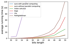
The experiment results in Figure 4 indicate that our algorithm is the most efficient algorithm to solve discrete logarithm problems. In particular, the running time of index calculus algorithm, baby step giant step algorithm, and PohligHellman algorithm are about 3 times, 7 times and 12 times that of our algorithms. The average running time of rho algorithm is far more than 20 times that of our algorithm.
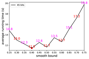
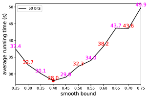
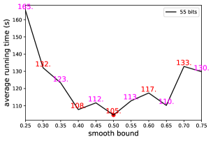
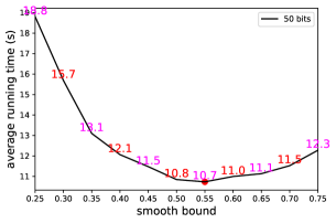
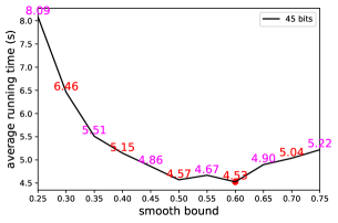
The third experiment focuses on the minimum of average running time. According to the experiment results in the first experiment, the average running time may be minimal when the smoothness bound is . To explore the minimum of the average running time, the smooth bounds are set to be , , , , , , , , , , where . The bit length is from 40 to 55 with step size 5. Many random discrete logarithm problems are generated and average running time of solving these discrete logarithm problems are shown in Fig 6.
The experiment results in Fig. 6 demonstrate obvious trends. First, the average running time decreases and then increases after a specific value as the smoothness bound increases from to , where . For example, the average running time of index calculus algorithm decreases when smoothness bound is smaller than . And then, the average running time of index calculus algorithm increases when smoothness bound is larger than . Second, our algorithm is faster than index calculus algorithm. In particular, when solving random discrete logarithm problems, the minimal average running time of index calculus algorithm is three times that of our algorithm. For example, the minimal average running time of index calculus algorithm is about 105s when the bit length is 55 bits. The minimal average running time of our algorithm is only about 1/3 (105/35.3) that of index calculus algorithm when the bit length is 55 bits. Third, the value of smoothness bound that makes the average running time minimal is become larger as the bit length increase. For example, the average running time is minimal of all algorithms when smoothness bounds is if the bit length is 40. However, the average running time is minimal of our algorithm and index calculus algorithm when smoothness bounds is and respectively if the bit length is 55.
The fourth experiment compares the average running time when the bit length is large. In particular, bit length is from 50 bits to 75 bits with step size 5. As demonstrated in the third experiment, the smoothness bound has large influence on the average running time. For the index calculus algorithm, the average running time is minimal when smoothness bound is , where . And for our algorithm, the average running time is minimal when smoothness bound is . Thus, in the fourth experiment, smoothness bounds of index calculus algorithm and our algorithm are and , respectively. Many random discrete logarithm problems are generated and the average running time of solving these problems is shown in Fig. 5.

According to the experiment results in Fig. 5, the computing speed of our algorithm is higher than that of index calculus algorithm. As the bit length becomes large, the difference on average running time becomes large too, which indicates that the performance of our algorithm becomes more better than the performance of the state-of-the-art index calculus algorithm.

(a) Index Calculus Algorithm


(b) Ours without Parallel Computing


(c) Ours with Parallel Computing
To demonstrate that our algorithm could be much faster than the state-of-the-art index calculus algorithm, we randomly set smooth bound to be
| (32) |
and
| (33) |
for index calculus algorithm and our algorithm. The comparison of average running time is shown in Table IV and the comparison indicates that our algorithm could be 30 times faster than the state-of-the-art index calculus algorithm.
| bit length | |||||
| 30 bits | 40 bits | 50 bits | 60 bits | 70 bits | |
| index calculus algorithm | 0.3s | 5.36s | 114.77s | 1707.66s | 75426.04s |
| our algorithm | 0.15s | 1.32s | 11.67s | 163.46s | 2211.92s |
| times | 2 | 4.1 | 9.8 | 10.4 | 34.1 |
In brief, our algorithm is compared with classical and state-of-the-art algorithms comprehensively, and the comparison indicates that our algorithm is better than existing algorithms.
VI Conclusion
In this paper, we propose the double index calculus algorithm to solve the discrete logarithm problem in the finite prime field. Our algorithm is faster than the fastest algorithm available. We give theoretical analyses and perform experiments to back up our claims. Empirical experiment results indicate that our algorithm could be more than 30 times faster than the fastest algorithm available when the bit length of the size of the prime field is large. Our improvement in solving the discrete logarithm problem in the finite prime field may influence how researchers choose security parameters of cryptography schemes whose security is based on the discrete logarithm problem.
References
- [1] W. Diffie and M. E. Hellman, “New directions in cryptography,” IEEE Transactions on Information Theory, vol. 22, no. 6, pp. 644–654, 1976.
- [2] R. Cramer and V. Shoup, “A practical public key cryptosystem provably secure against adaptive chosen ciphertext attack,” in Advances in Cryptology — CRYPTO ’98, H. Krawczyk, Ed. Berlin, Heidelberg: Springer Berlin Heidelberg, 1998, pp. 13–25.
- [3] T. Elgamal, “A public key cryptosystem and a signature scheme based on discrete logarithms,” IEEE Transactions on Information Theory, vol. 31, no. 4, pp. 469–472, 1985.
- [4] D. Johnson, A. Menezes, and S. Vanstone, “The elliptic curve digital signature algorithm (ecdsa),” International journal of information security, vol. 1, no. 1, pp. 36–63, 2001.
- [5] F. Li, D. Zhong, and T. Takagi, “Efficient deniably authenticated encryption and its application to e-mail,” IEEE Transactions on Information Forensics and Security, vol. 11, no. 11, pp. 2477–2486, 2016.
- [6] D. Shanks, “Class number, a theory of factorization, and genera,” in Proc. of Symp. Math. Soc., 1971, vol. 20, 1971, pp. 41–440. [Online]. Available: https://doi.org/10.1090/pspum/020/0316385
- [7] S. Pohlig and M. Hellman, “An improved algorithm for computing logarithms overgf(p)and its cryptographic significance (corresp.),” IEEE Transactions on Information Theory, vol. 24, no. 1, pp. 106–110, 1978.
- [8] J. M. Pollard, “Monte carlo methods for index computation (mod) p,” Mathematics of Computation, vol. 32, no. 143, pp. 918–924, 1978.
- [9] M. Kraitchik, Théorie des nombres. Gauthier-Villars, 1922, vol. 1.
- [10] ——, Recherches sur la théorie des nombres. Gauthier-Villars, 1924, vol. 1.
- [11] E. Western Alfred and J. Miller, “Tables of indices and primitive roots,” the Royal Society Mathematical Tables, vol. 9, 1968.
- [12] L. Adleman, “A subexponential algorithm for the discrete logarithm problem with applications to cryptography,” in 2013 IEEE 54th Annual Symposium on Foundations of Computer Science. Los Alamitos, CA, USA: IEEE Computer Society, oct 1979, pp. 55–60. [Online]. Available: https://doi.ieeecomputersociety.org/10.1109/SFCS.1979.2
- [13] R. C. Merkle, Secrecy, authentication, and public key systems. Stanford university, 1979.
- [14] L. Adleman, “A subexponential algorithm for the discrete logarithm problem with applications to cryptography,” in 2013 IEEE 54th Annual Symposium on Foundations of Computer Science. Los Alamitos, CA, USA: IEEE Computer Society, oct 1979, pp. 55–60. [Online]. Available: https://doi.ieeecomputersociety.org/10.1109/SFCS.1979.2
- [15] L. M. Adleman and J. DeMarrais, “A subexponential algorithm for discrete logarithms over all finite fields,” Mathematics of Computation, vol. 61, no. 203, pp. 1–15, 1993.
- [16] D. M. Gordon, “Discrete logarithms in $gf ( p )$ using the number field sieve,” SIAM Journal on Discrete Mathematics, vol. 6, no. 1, pp. 124–138, 1993. [Online]. Available: https://doi.org/10.1137/0406010
- [17] L. M. Adleman and M.-D. A. Huang, “Function field sieve method for discrete logarithms over finite fields,” Information and Computation, vol. 151, no. 1, pp. 5–16, 1999. [Online]. Available: https://www.sciencedirect.com/science/article/pii/S0890540198927614
- [18] A. Sutherland, “Index calculus, smooth numbers, and factoring integers,” Website, 2023, https://math.mit.edu/classes/18.783/2015/LectureNotes11.pdf.
- [19] D. Coppersmith, “Fast evaluation of logarithms in fields of characteristic two,” IEEE Transactions on Information Theory, vol. 30, no. 4, pp. 587–594, 1984.
- [20] A. Shuaibu Maianguwa, “A survey of discrete logarithm algorithms in finite fields,” vol. 5, pp. 215 – 224, 01 2019.
- [21] R. Barbulescu, P. Gaudry, A. Joux, and E. Thomé, “A heuristic quasi-polynomial algorithm for discrete logarithm in finite fields of small characteristic,” in Advances in Cryptology – EUROCRYPT 2014, P. Q. Nguyen and E. Oswald, Eds. Berlin, Heidelberg: Springer Berlin Heidelberg, 2014, pp. 1–16.
- [22] G. Adj, A. Menezes, T. Oliveira, and F. Rodríguez-Henríquez, “Weakness of and for discrete logarithm cryptography,” Finite Fields and Their Applications, vol. 32, pp. 148–170, 2015, special Issue : Second Decade of FFA. [Online]. Available: https://www.sciencedirect.com/science/article/pii/S1071579714001294
- [23] J. Detrey, P. Gaudry, and M. Videau, “Relation collection for the function field sieve,” in 2013 IEEE 21st Symposium on Computer Arithmetic, 2013, pp. 201–210.
- [24] A. Joux, “Faster index calculus for the medium prime case application to 1175-bit and 1425-bit finite fields,” in Advances in Cryptology – EUROCRYPT 2013, T. Johansson and P. Q. Nguyen, Eds. Berlin, Heidelberg: Springer Berlin Heidelberg, 2013, pp. 177–193.
- [25] M. Mukhopadhyay, P. Sarkar, S. Singh, and E. Thome, “New discrete logarithm computation for the medium prime case using the function field sieve,” Cryptology ePrint Archive, Paper 2020/113, 2020, https://eprint.iacr.org/2020/113. [Online]. Available: https://eprint.iacr.org/2020/113