Increasing Both Batch Size and Learning Rate Accelerates Stochastic Gradient Descent

Abstract

The performance of mini-batch stochastic gradient descent (SGD) strongly depends on setting the batch size and learning rate to minimize the empirical loss in training the deep neural network. In this paper, we present theoretical analyses of mini-batch SGD with four schedulers: (i) constant batch size and decaying learning rate scheduler, (ii) increasing batch size and decaying learning rate scheduler, (iii) increasing batch size and increasing learning rate scheduler, and (iv) increasing batch size and warm-up decaying learning rate scheduler. We show that mini-batch SGD using scheduler (i) does not always minimize the expectation of the full gradient norm of the empirical loss, whereas it does using any of schedulers (ii), (iii), and (iv). Furthermore, schedulers (iii) and (iv) accelerate mini-batch SGD. The paper also provides numerical results of supporting analyses showing that using scheduler (iii) or (iv) minimizes the full gradient norm of the empirical loss faster than using scheduler (i) or (ii).

1 Introduction

Mini-batch stochastic gradient descent (SGD) (Robbins & Monro, 1951; Zinkevich, 2003; Nemirovski et al., 2009; Ghadimi & Lan, 2012; 2013) is a simple and useful deep-learning optimizer for finding appropriate parameters of a deep neural network (DNN) in the sense of minimizing the empirical loss defined by the mean of nonconvex loss functions corresponding to the training set.

The performance of mini-batch SGD strongly depends on how the batch size and learning rate are set. In particular, increasing batch size (Byrd et al., 2012; Balles et al., 2016; De et al., 2017; Smith et al., 2018; Goyal et al., 2018; Shallue et al., 2019; Zhang et al., 2019) is useful for training DNNs with mini-batch SGD. In (Smith et al., 2018), it was numerically shown that using an enormous batch size leads to a reduction in the number of parameter updates.

Decaying a learning rate (Wu et al., 2014; Ioffe & Szegedy, 2015; Loshchilov & Hutter, 2017; Hundt et al., 2019) is also useful for training DNNs with mini-batch SGD. In (Chen et al., 2020), theoretical results indicated that running SGD with a diminishing learning rate $\eta_{t}=O(1/t)$ and a large batch size for sufficiently many steps leads to convergence to a stationary point. A practical example of a decaying learning rate with $\eta_{t+1}\leq\eta_{t}$ for all $t\in\mathbb{N}$ is a constant learning rate $\eta_{t}=\eta>0$ for all $t\in\mathbb{N}$. However, convergence of SGD with a constant learning rate is not guaranteed (Scaman & Malherbe, 2020). Other practical learning rates have been presented for training DNNs, including cosine annealing (Loshchilov & Hutter, 2017), cosine power annealing (Hundt et al., 2019), step decay (Lu, 2024), exponential decay (Wu et al., 2014), polynomial decay (Chen et al., 2018), and linear decay (Liu et al., 2020).

Contribution: The main contribution of the present paper is its theoretical analyses of mini-batch SGD with batch size and learning rate schedulers used in practice satisfying the following inequality:

$$\min_{t\in[0:T-1]}\mathbb{E}\left[\|\nabla f(\bm{\theta}_{t})\|\right]\leq\bigg{\{}\frac{2(f(\bm{\theta}_{0})-f^{\star})}{2-L_{n}\eta_{\max}}\underbrace{\frac{1}{\sum_{t=0}^{T-1}\eta_{t}}}_{B_{T}}+\frac{L_{n}\sigma^{2}}{2-L_{n}\eta_{\max}}\underbrace{\frac{1}{\sum_{t=0}^{T-1}\eta_{t}}\sum_{t=0}^{T-1}\frac{\eta_{t}^{2}}{b_{t}}}_{V_{T}}\bigg{\}}^{\frac{1}{2}},$$

where $f$ is the empirical loss for $n$ training samples having $L_{n}$-Lipschitz continuous gradient $\nabla f$ and lower bound $f^{\star}$, $\sigma^{2}$ is an upper bound on the variance of the mini-batch stochastic gradient, and $(\bm{\theta}_{t})_{t=0}^{T-1}$ is the sequence generated by mini-batch SGD with batch size $b_{t}$, learning rate $\eta_{t}\in[\eta_{\min},\eta_{\max}]\subset[0,\frac{2}{L_{n}})$, and total number of steps to train a DNN $T$.

Scheduler	$B_{T}$	$V_{T}$	$O(\sqrt{B_{T}+V_{T}})$
Case (i) (Theorem 3.1; Section 3.1)	$\displaystyle{\frac{H_{1}}{T}}$	$\displaystyle{\frac{H_{2}}{b}+\frac{H_{7}}{bT}}$	$\displaystyle{O\left(\sqrt{\frac{1}{T}+\frac{1}{b}}\right)}$
$b_{t}\colon$Constant; $\eta_{t}\colon$Decay
Case (ii) (Theorem 3.2; Section 3.2)	$\displaystyle{\frac{H_{3}}{T}}$	$\displaystyle{\frac{H_{4}}{b_{0}T}}$	$\displaystyle{O\left(\frac{1}{\sqrt{T}}\right),\text{ }O\left(\frac{1}{\sqrt{M}}\right)}$
$b_{t}\colon$Increase; $\eta_{t}\colon$Decay
Case (iii) (Theorem 3.3; Section 3.3)	$\displaystyle{\frac{H_{5}}{\gamma^{M}}}$	$\displaystyle{\frac{H_{6}}{b_{0}\gamma^{M}}}$	$\displaystyle{O\left(\frac{1}{\gamma^{\frac{M}{2}}}\right)}$ Remark:
$b_{t}\colon$Increase; $\eta_{t}\colon$Increase			$\frac{1}{\gamma^{\frac{M}{2}}}<\frac{1}{\sqrt{M}}$
Case (iv) (Theorem 3.4; Section 3.4)	$\displaystyle{\frac{H_{5}}{\gamma^{M}}\to\frac{H_{3}}{T}}$	$\displaystyle{\frac{H_{6}}{b_{0}\gamma^{M}}\to\frac{H_{4}}{b_{0}T}}$	$\displaystyle{O\left(\frac{1}{\gamma^{\frac{M}{2}}}\right)\to O\left(\frac{1}{\sqrt{T}}\right)}$
$b_{t}\colon$Increase; $\eta_{t}\colon$Increase $\to$ Decay

$H_{i}$ ($i\in[6]$) (resp. $H_{7}$) is a positive (resp. nonnegative) number depending on $\eta_{\min}$ and $\eta_{\max}$. $\gamma$ and $\delta$ are such that $1<\gamma^{2}<\delta$ (e.g., $\delta=2$ when batch size is doubly increasing every $E$ epochs). The total number of steps when batch size increases $M$ times is $T(M)=\sum_{m=0}^{M}\lceil\frac{n}{b_{m}}\rceil E\geq ME$.

(i) Using constant batch size $b_{t}=b$ and decaying learning rate $\eta_{t}$ (Theorem 3.1; Section 3.1): Using a constant batch size and practical decaying learning rates, such as constant, cosine-annealing, and polynomial decay learning rates, satisfies that, for a sufficiently large step $T$, the upper bound on $\min_{t\in[0:T-1]}\mathbb{E}[\|\nabla f(\bm{\theta}_{t})\|]$ becomes approximately $O(\frac{1}{\sqrt{b}})>0$, which implies that mini-batch SGD does not always converge to a stationary point of $f$. Meanwhile, the analysis indicates that using the cosine-annealing and polynomial decay learning rates decreases $\mathbb{E}[\|\nabla f(\bm{\theta}_{t})\|]$ faster than using a constant learning rate (see (7)), which is supported by the numerical results in Figure 1.

(ii) Using increasing batch size $b_{t}$ and decaying learning rate $\eta_{t}$ (Theorem 3.2; Section 3.2): Although convergence analyses of SGD were presented in (Vaswani et al., 2019; Fehrman et al., 2020; Scaman & Malherbe, 2020; Loizou et al., 2021; Wang et al., 2021; Khaled & Richtárik, 2023), providing the theoretical performance of mini-batch SGD with increasing batch sizes that have been used in practice may not be sufficient. The present paper shows that mini-batch SGD has an $O(\frac{1}{\sqrt{T}})$ rate of convergence. Increasing batch size every $E$ epochs makes the polynomial decay and linear learning rates become small at an early stage of training (Figure 2(a)). Meanwhile, the cosine-annealing and constant learning rates are robust to increasing batch sizes (Figure 2(a)). Hence, it is desirable for mini-batch SGD using increasing batch sizes to use the cosine-annealing and constant learning rates, which is supported by the numerical results in Figure 2.

(iii) Using increasing batch size $b_{t}$ and increasing learning rate $\eta_{t}$ (Theorem 3.3; Section 3.3): From Case (ii), when batch sizes increase, keeping learning rates large is useful for training DNNs. Hence, we are interested in verifying whether mini-batch SGD with both the batch sizes and learning rates increasing can train DNNs. Let us consider a scheduler doubly increasing batch size (i.e., $\delta=2$). We set $\gamma>1$ such that $\gamma<\sqrt{\delta}=\sqrt{2}$ and we set an increasing learning rate scheduler such that the learning rate is multiplied by $\gamma$ every $E$ epochs (Figure 3(a)). This paper shows that, when batch size increases $M$ times, mini-batch SGD has an $O(\gamma^{-\frac{M}{2}})$ convergence rate that is better than the $O(\frac{1}{\sqrt{M}})$ convergence rate in Case (ii). That is, increasing both batch size and learning rate accelerates mini-batch SGD. We give practical results (Figure 3(b); $\delta=2$ and Figure 5(b); $\delta=3,4$) such that Case (iii) decreases $\|\nabla f(\bm{\theta}_{t})\|$ faster than Case (ii) and tripling and quadrupling batch sizes ($\delta=3,4$) decrease $\|\nabla f(\bm{\theta}_{t})\|$ faster than doubly increasing batch sizes ($\delta=2$).

(iv) Using increasing batch size $b_{t}$ and warm-up decaying learning rate $\eta_{t}$ (Theorem 3.4; Section 3.4): One way to guarantee fast convergence of mini-batch SGD with increasing batch sizes is to increase learning rates (acceleration period; Case (iii)) during the first epochs and then decay the learning rates (convergence period; Case (ii)), that is, to use a decaying learning rate with warm-up (He et al., 2016; Vaswani et al., 2017; Goyal et al., 2018; Gotmare et al., 2019; He et al., 2019). We give numerical results (Figure 4) indicating that using mini-batch SGD with increasing batch sizes and decaying learning rates with a warm-up minimizes $\|\nabla f(\bm{\theta}_{t})\|$ faster than using a constant learning rate in Case (ii) or increasing learning rates in Case (iii).

2 Mini-batch SGD for empirical risk minimization

2.1 Empirical risk minimization

Let $\bm{\theta}\in\mathbb{R}^{d}$ be a parameter of a deep neural network; let $S=\{(\bm{x}_{1},\bm{y}_{1}),\ldots,(\bm{x}_{n},\bm{y}_{n})\}$ be the training set, where data point $\bm{x}_{i}$ is associated with label $\bm{y}_{i}$; and let $f_{i}(\cdot):=f(\cdot;(\bm{x}_{i},\bm{y}_{i}))\colon\mathbb{R}^{d}\to\mathbb{R}_{+}$ be the loss function corresponding to the $i$-th labeled training data $(\bm{x}_{i},\bm{y}_{i})$. Empirical risk minimization (ERM) minimizes the empirical loss defined for all $\bm{\theta}\in\mathbb{R}^{d}$ as $f(\bm{\theta})=\frac{1}{n}\sum_{i\in[n]}f_{i}(\bm{\theta})$. This paper considers the following stationary point problem: Find $\bm{\theta}^{\star}\in\mathbb{R}^{d}$ such that $\nabla f(\bm{\theta}^{\star})=\bm{0}$.

We assume that the loss functions $f_{i}$ ($i\in[n]$) satisfy the conditions in the following assumption (see Appendix A for definitions of functions, mappings, and notation used in this paper).

Assumption 2.1.

Let $n$ be the number of training samples and let $L_{i}>0$ ($i\in[n]$).

(A1) $f_{i}\colon\mathbb{R}^{d}\to\mathbb{R}$ ($i\in[n]$) is differentiable and $L_{i}$-smooth, and $f_{i}^{\star}:=\inf\{f_{i}(\bm{\theta})\colon\bm{\theta}\in\mathbb{R}^{d}\}\in\mathbb{R}$.

(A2) Let $\xi$ be a random variable that is independent of $\bm{\theta}\in\mathbb{R}^{d}$. $\nabla f_{\xi}\colon\mathbb{R}^{d}\to\mathbb{R}^{d}$ is the stochastic gradient of $\nabla f$ such that (i) for all $\bm{\theta}\in\mathbb{R}^{d}$, $\mathbb{E}_{\xi}[\nabla f_{\xi}(\bm{\theta})]=\nabla f(\bm{\theta})$ and (ii) there exists $\sigma\geq 0$ such that, for all $\bm{\theta}\in\mathbb{R}^{d}$, $\mathbb{V}_{\xi}[\nabla f_{\xi}(\bm{\theta})]=\mathbb{E}_{\xi}[\|\nabla f_{\xi}(\bm{\theta})-\nabla f(\bm{\theta})\|^{2}]\leq\sigma^{2}$, where $\mathbb{E}_{\xi}[\cdot]$ denotes expectation with respect to $\xi$.

(A3) Let $b\in\mathbb{N}$ such that $b\leq n$; and let $\bm{\xi}=(\xi_{1},\xi_{2},\cdots,\xi_{b})^{\top}$ comprise $b$ independent and identically distributed variables and be independent of $\bm{\theta}\in\mathbb{R}^{d}$. The full gradient $\nabla f(\bm{\theta})$ is estimated as the following mini-batch gradient at $\bm{\theta}$: $\nabla f_{B}(\bm{\theta}):=\frac{1}{b}\sum_{i=1}^{b}\nabla f_{\xi_{i}}(\bm{\theta})$.

2.2 Mini-batch SGD

Given the $t$-th approximated parameter $\bm{\theta}_{t}\in\mathbb{R}^{d}$ of the deep neural network, mini-batch SGD uses $b_{t}$ loss functions $f_{\xi_{t,1}},f_{\xi_{t,2}},\cdots,f_{\xi_{t,b_{t}}}$ randomly chosen from $\{f_{1},f_{2},\cdots,f_{n}\}$ at each step $t$, where $\bm{\xi}_{t}=(\xi_{t,1},\xi_{t,2},\cdots,\xi_{t,b_{t}})^{\top}$ is independent of $\bm{\theta}_{t}$ and $b_{t}$ is a batch size satisfying $b_{t}\leq n$. The pseudo-code of the algorithm is shown as Algorithm 1.

Algorithm 1 Mini-batch SGD algorithm

0:  $\bm{\theta}_{0}\in\mathbb{R}^{d}$ (initial point), $b_{t}>0$ (batch size), $\eta_{t}>0$ (learning rate), $T\geq 1$ (steps)

0:  $(\bm{\theta}_{t})\subset\mathbb{R}^{d}$

1:  for $t=0,1,\ldots,T-1$ do

2:      $\nabla f_{B_{t}}(\bm{\theta}_{t}):=\frac{1}{b_{t}}\sum_{i=1}^{b_{t}}\nabla f_{\xi_{t,i}}(\bm{\theta}_{t})$

3:      $\bm{\theta}_{t+1}:=\bm{\theta}_{t}-\eta_{t}\nabla f_{B_{t}}(\bm{\theta}_{t})$

4:  end for

The following lemma can be proved using Proposition A.1, Assumption 2.1, and the descent lemma (Beck, 2017, Lemma 5.7): for all $\bm{\theta}_{1},\bm{\theta}_{2}\in\mathbb{R}^{d}$, $f(\bm{\theta}_{2})\leq f(\bm{\theta}_{1})+\langle\nabla f(\bm{\theta}_{1}),\bm{\theta}_{2}-\bm{\theta}_{1}\rangle+\frac{L_{n}}{2}\|\bm{\theta}_{2}-\bm{\theta}_{1}\|^{2}$, where Assumption 2.1(A1) ensures that $f$ is $L_{n}$-smooth ($L_{n}:=\frac{1}{n}\sum_{i\in[n]}L_{i}$). The proof itself is given in Appendix A.1.

Lemma 2.1.

Suppose that Assumption 2.1 holds and consider the sequence $(\bm{\theta}_{t})$ generated by Algorithm 1 with $\eta_{t}\in[\eta_{\min},\eta_{\max}]\subset[0,\frac{2}{L_{n}})$ satisfying $\sum_{t=0}^{T-1}\eta_{t}\neq 0$, where $L_{n}:=\frac{1}{n}\sum_{i\in[n]}L_{i}$ and $f^{\star}:=\frac{1}{n}\sum_{i\in[n]}f_{i}^{\star}$. Then, for all $T\in\mathbb{N}$,

$$\min_{t\in[0:T-1]}\mathbb{E}\left[\|\nabla f(\bm{\theta}_{t})\|^{2}\right]\leq\frac{2(f(\bm{\theta}_{0})-f^{\star})}{2-L_{n}\eta_{\max}}\frac{1}{\sum_{t=0}^{T-1}\eta_{t}}+\frac{L_{n}\sigma^{2}}{2-L_{n}\eta_{\max}}\frac{\sum_{t=0}^{T-1}\eta_{t}^{2}b_{t}^{-1}}{\sum_{t=0}^{T-1}\eta_{t}},$$

where $\mathbb{E}$ denotes the total expectation, defined by $\mathbb{E}:=\mathbb{E}_{\bm{\xi}_{0}}\mathbb{E}_{\bm{\xi}_{1}}\cdots\mathbb{E}_{\bm{\xi}_{t}}$.

3 Convergence Analysis of Mini-batch SGD

3.1 Constant batch size and decaying learning rate scheduler

This section considers a constant batch size and a decaying learning rate:

$$b_{t}=b\text{ }(t\in\mathbb{N})\quad\text{and}\quad\eta_{t+1}\leq\eta_{t}\text{ }(t\in\mathbb{N}).$$ (1)

Let $p>0$ and $T,E\in\mathbb{N}$; and let $\eta_{\min}$ and $\eta_{\max}$ satisfy $0\leq\eta_{\min}\leq\eta_{\max}$. Examples of decaying learning rates are as follows: for all $t\in[0:T]$,

$$\text{[Constant LR] }\eta_{t}=\eta_{\max},$$ (2)

$$\text{[Diminishing LR] }\eta_{t}=\frac{\eta_{\max}}{\sqrt{t+1}},$$ (3)

$$\text{[Cosine-annealing LR] }\eta_{t}=\eta_{\min}+\frac{\eta_{\max}-\eta_{\min}}{2}\left(1+\cos\left\lfloor\frac{t}{K}\right\rfloor\frac{\pi}{E}\right),$$ (4)

$$\text{[Polynomial Decay LR] }\eta_{t}=(\eta_{\max}-\eta_{\min})\left(1-\frac{t}{T}\right)^{p}+\eta_{\min},$$ (5)

where $K=\lceil\frac{n}{b}\rceil$ is the number of steps per epoch, $E$ is the total number of epochs, and the number of steps $T$ in (4) is given by $T=KE$. A simple, practical decaying learning rate is the constant learning rate defined by (2). A decaying learning rate used in theoretical analyses of deep-learning optimizers is the diminishing learning rate defined by (3). The cosine-annealing learning rate defined by (4) and the linear learning rate defined by (5) with $p=1$ (i.e., an example of a polynomial decay learning rate) are used in practice. Note that the cosine-annealing learning rate is updated each epoch, whereas the polynomial decay learning rate is updated each step.

Lemma 2.1 leads to the following (the proof of the theorem is given in Appendix A.2).

Theorem 3.1 (Upper bound on $\min_{t}\mathbb{E}\|\nabla f(\bm{\theta}_{t})\|^{2}$ for SGD using (1)).

Under the assumptions in Lemma 2.1, Algorithm 1 using (1) satisfies that, for all $T\in\mathbb{N}$,

$$\min_{t\in[0:T-1]}\mathbb{E}\left[\|\nabla f(\bm{\theta}_{t})\|^{2}\right]\leq\frac{2(f(\bm{\theta}_{0})-f^{\star})}{2-L_{n}\eta_{\max}}\underbrace{\frac{1}{\sum_{t=0}^{T-1}\eta_{t}}}_{B_{T}}+\frac{L_{n}\sigma^{2}}{2-L_{n}\eta_{\max}}\underbrace{\frac{\sum_{t=0}^{T-1}\eta_{t}^{2}}{b\sum_{t=0}^{T-1}\eta_{t}}}_{V_{T}},$$

where $\eta$, $p$, $\eta_{\min}$, $\eta_{\max}$, $K$, and $E$ are the parameters used in (2)–(5), $T=KE=\lceil\frac{n}{b}\rceil E$ for Polynomial LR (5),

$$\begin{split}B_{T}\leq\begin{cases}\displaystyle{\frac{1}{\eta_{\max}T}}&\text{ {\em[Constant LR (\ref{constant})]}}\\ \displaystyle{\frac{1}{2\eta_{\max}(\sqrt{T+1}-1)}}&\text{ {\em[Diminishing LR (\ref{diminishing})]}}\\ \displaystyle{\frac{2}{(\eta_{\min}+\eta_{\max})T}}&\text{ {\em[Cosine LR (\ref{cosine})]}}\\ \displaystyle{\frac{p+1}{(p\eta_{\min}+\eta_{\max})T}}&\text{ {\em[Polynomial LR (\ref{polynomial})]}},\end{cases}\end{split}$$ (6)

$$V_{T}\leq\begin{cases}\displaystyle{\frac{\eta_{\max}}{b}}&\text{ {\em[Constant LR (\ref{constant})]}}\\ \displaystyle{\frac{\eta_{\max}(1+\log T)}{2b(\sqrt{T+1}-1)}}&\text{ {\em[Diminishing LR (\ref{diminishing})]}}\\ \displaystyle{\frac{3\eta_{\min}^{2}+2\eta_{\min}\eta_{\max}+3\eta_{\max}^{2}}{4(\eta_{\min}+\eta_{\max})b}+\frac{\eta_{\max}-\eta_{\min}}{bT}}&\text{ {\em[Cosine LR (\ref{cosine})]}}\\ \displaystyle{\frac{2p^{2}\eta_{\min}^{2}+2p\eta_{\min}\eta_{\max}+(p+1)\eta_{\max}^{2}}{(2p+1)(p\eta_{\min}+\eta_{\max})b}+\frac{(p+1)(\eta_{\max}^{2}-\eta_{\min}^{2})}{(p\eta_{\min}+\eta_{\max})bT}}&\text{ {\em[Polynomial LR (\ref{polynomial})]}}.\end{cases}$$

Let us consider using Constant LR (2), Cosine LR (4), or Polynomial LR (5). Theorem 3.1 indicates that the bias term including $B_{T}$ converges to $0$ as $O(\frac{1}{T})$, whereas the variance term including $V_{T}$ does not always converge to $0$. Hence, the upper bound on $\min_{t\in[0:T-1]}\mathbb{E}[\|\nabla f(\bm{\theta}_{t})\|^{2}]$ does not converge to $0$. In fact, Theorem 3.1 with $\eta=\eta_{\max}$ and $\eta_{\min}=0$ implies that

$$\limsup_{T\to+\infty}\min_{t\in[0:T-1]}\mathbb{E}\left[\|\nabla f(\bm{\theta}_{t})\|^{2}\right]\leq\frac{L_{n}\sigma^{2}}{(2-L_{n}\eta)b}\times\begin{cases}\eta&\text{ [Constant LR (\ref{constant})]}\\ \displaystyle{\frac{3\eta}{4}}&\text{ [Cosine LR (\ref{cosine})]}\\ \displaystyle{\frac{(p+1)\eta}{(2p+1)}}&\text{ [Polynomial LR (\ref{polynomial})]}.\end{cases}$$ (7)

Since $\frac{3\eta}{4}<\eta$ and $\frac{(p+1)\eta}{(2p+1)}<\eta$ ($p>0$), using the cosine-annealing learning rate or the polynomial decay learning rate is better than using the constant learning rate in the sense of minimizing the upper bound on $\min_{t\in[0:T-1]}\mathbb{E}[\|\nabla f(\bm{\theta}_{t})\|^{2}]$. Theorem 3.1 also indicates that Algorithm 1 using Diminishing LR (3) converges to $0$ with the convergence rate $\min_{t\in[0:T-1]}\mathbb{E}[\|\nabla f(\bm{\theta}_{t})\|]=O(\frac{\sqrt{\log T}}{T^{\frac{1}{4}}})$. However, since Diminishing LR (3) defined by $\eta_{t}=\frac{\eta}{\sqrt{t+1}}$ decays rapidly (see Figure 1(a)), it would not be useful for training DNNs in practice.

3.2 Increasing batch size and decaying learning rate scheduler

An increasing batch size is used to train DNNs in practice (Byrd et al., 2012; Balles et al., 2016; De et al., 2017; Smith et al., 2018; Goyal et al., 2018). This section considers an increasing batch size and a decaying learning rate following one of (2)–(5):

$$b_{t}\leq b_{t+1}\text{ }(t\in\mathbb{N})\quad\text{and}\quad\eta_{t+1}\leq\eta_{t}\text{ }(t\in\mathbb{N}).$$ (8)

Examples of $b_{t}$ are, for example, for all $m\in[0:M]$ and all $t\in S_{m}=\mathbb{N}\cap[\sum_{k=0}^{m-1}K_{k}E_{k},\sum_{k=0}^{m}K_{k}E_{k})$ ($S_{0}:=\mathbb{N}\cap[0,K_{0}E_{0})$),

$$\text{[Polynomial growth BS] }b_{t}=\left(am\left\lceil\frac{t}{\sum_{k=0}^{m}K_{k}E_{k}}\right\rceil+b_{0}\right)^{c},$$ (9)

$$\text{[Exponential growth BS] }b_{t}=\gamma^{m\left\lceil\frac{t}{\sum_{k=0}^{m}K_{k}E_{k}}\right\rceil}b_{0},$$ (10)

where $a\in\mathbb{R}_{++}$, $c,\gamma>1$, and $E_{m}$ and $K_{m}$ are the numbers of, respectively, epochs and steps per epoch when the batch size is $(am+b_{0})^{c}$ or $\gamma^{m}b_{0}$. For example, the exponential growth batch size defined by (10) with $\gamma=2$ makes batch size double each $E_{m}$ epochs. We may modify the parameters $a$ and $\gamma$ to $a_{t}$ and $\gamma_{t}$ monotone increasing with $t$. The total number of steps for the batch size to increase $M$ times is $T=\sum_{m=0}^{M}K_{m}E_{m}$. An analysis of Algorithm 1 with a constant batch size $b_{t}=b$ and decaying learning rates satisfying (8) is given in Section 3.1.

Lemma 2.1 leads to the following them (the proof of the theorem and the result for Polynomial BS (9) are given in Appendix A.2).

Theorem 3.2 (Convergence rate of SGD using (8)).

Under the assumptions in Lemma 2.1, Algorithm 1 using (8) satisfies that, for all $M\in\mathbb{N}$,

$$\min_{t\in[0:T-1]}\mathbb{E}\left[\|\nabla f(\bm{\theta}_{t})\|^{2}\right]\leq\frac{2(f(\bm{\theta}_{0})-f^{\star})}{2-L_{n}\eta_{\max}}\underbrace{\frac{1}{\sum_{t=0}^{T-1}\eta_{t}}}_{B_{T}}+\frac{L_{n}\sigma^{2}}{2-L_{n}\eta_{\max}}\underbrace{\frac{1}{\sum_{t=0}^{T-1}\eta_{t}}\sum_{t=0}^{T-1}\frac{\eta_{t}^{2}}{b_{t}}}_{V_{T}},$$

where $T=\sum_{m=0}^{M}K_{m}E_{m}$, $E_{\max}=\sup_{M\in\mathbb{N}}\sup_{m\in[0:M]}E_{m}<+\infty$, $K_{\max}=\sup_{M\in\mathbb{N}}\sup_{m\in[0:M]}K_{m}<+\infty$, $B_{T}$ is defined as in (6), and $V_{T}$ is bounded as

$$V_{T}\leq\begin{cases}\displaystyle{\frac{\gamma\eta K_{\max}E_{\max}}{(\gamma-1)b_{0}T}}&\text{ {\em[Constant LR (\ref{constant})]}}\\ \displaystyle{\frac{\gamma\eta K_{\max}E_{\max}}{2(\gamma-1)b_{0}(\sqrt{T+1}-1)}}&\text{ {\em[Diminishing LR (\ref{diminishing})]}}\\ \displaystyle{\frac{2\gamma\eta_{\max}^{2}K_{\max}E_{\max}}{(\gamma-1)(\eta_{\min}+\eta_{\max})b_{0}T}}&\text{ {\em[Cosine LR (\ref{cosine})]}}\\ \displaystyle{\frac{(p+1)\gamma\eta_{\max}^{2}K_{\max}E_{\max}}{(\gamma-1)(\eta_{\max}+\eta_{\min}p)b_{0}T}}&\text{ {\em[Polynomial LR (\ref{polynomial})]}}.\end{cases}\text{ {\em([Exponential BS (\ref{exponential_bs})])}}$$

That is, Algorithm 1 using Exponential BS (10) has the convergence rate

$$\min_{t\in[0:T-1]}\mathbb{E}\left[\|\nabla f(\bm{\theta}_{t})\|\right]=\begin{cases}\displaystyle{O\left(\frac{1}{\sqrt{T}}\right)}&\text{ {\em[Constant LR (\ref{constant}), Cosine LR (\ref{cosine}), Polynomial LR (\ref{polynomial})]}}\\ \displaystyle{O\left(\frac{1}{T^{\frac{1}{4}}}\right)}&\text{ {\em[Diminishing LR (\ref{diminishing})]}}.\end{cases}$$

Theorem 3.2 (Theorem A.1) indicates that, with increasing batch sizes such as Polynomial BS (9) and Exponential BS (10), Algorithm 1 using each of Constant LR (2), Cosine LR (4), and Polynomial LR (5) has the convergence rate $O(\frac{1}{\sqrt{T}})$, in contrast to Theorem 3.1.

3.3 Increasing batch size and increasing learning rate scheduler

This section considers an increasing batch size and an increasing learning rate:

$$b_{t}\leq b_{t+1}\text{ }(t\in\mathbb{N})\quad\text{and}\quad\eta_{t}\leq\eta_{t+1}\text{ }(t\in\mathbb{N}).$$ (11)

Example of $b_{t}$ and $\eta_{t}$ satisfying (11) is as follows: for all $m\in[0,M]$ and all $t\in S_{m}=\mathbb{N}\cap[\sum_{k=0}^{m-1}K_{k}E_{k},\sum_{k=0}^{m}K_{k}E_{k})$ ($S_{0}=\mathbb{N}\cap[0,K_{0}E_{0})$),

$$\text{[Exponential growth BS and LR] }b_{t}=\delta^{m\left\lceil\frac{t}{\sum_{k=0}^{m}K_{k}E_{k}}\right\rceil}b_{0},\text{ }\eta_{t}=\gamma^{m\left\lceil\frac{t}{\sum_{k=0}^{m}K_{k}E_{k}}\right\rceil}\eta_{0},$$ (12)

where $\delta,\gamma>1$ such that $\gamma^{2}<\delta$; and $E_{m}$ and $K_{m}$ are defined as in (10). We may modify the parameters $\gamma$ and $\delta$ to be monotone increasing parameters in $t$. The total number of steps when both batch size and learning rate increase $M$ times is $T=\sum_{m=0}^{M}K_{m}E_{m}$.

Lemma 2.1 leads to the following theorem (the proof of the theorem and the result for Polynomial growth BS and LR (25) are given in Appendix A.2).

Theorem 3.3 (Convergence rate of SGD using (11)).

Under the assumptions in Lemma 2.1, Algorithm 1 using (11) satisfies that, for all $M\in\mathbb{N}$,

$$\min_{t\in[0:T-1]}\mathbb{E}\left[\|\nabla f(\bm{\theta}_{t})\|^{2}\right]\leq\frac{2(f(\bm{\theta}_{0})-f^{\star})}{2-L_{n}\eta_{\max}}\underbrace{\frac{1}{\sum_{t=0}^{T-1}\eta_{t}}}_{B_{T}}+\frac{L_{n}\sigma^{2}}{2-L_{n}\eta_{\max}}\underbrace{\frac{1}{\sum_{t=0}^{T-1}\eta_{t}}\sum_{t=0}^{T-1}\frac{\eta_{t}^{2}}{b_{t}}}_{V_{T}},$$

where $T$, $E_{\max}$, and $K_{\max}$ are defined as in Theorem 3.2, $E_{\min}=\inf_{M\in\mathbb{N}}\inf_{m\in[0:M]}E_{m}<+\infty$, $K_{\min}=\inf_{M\in\mathbb{N}}\inf_{m\in[0:M]}K_{m}<+\infty$, $\hat{\gamma}=\frac{\gamma^{2}}{\delta}<1$,

$$B_{T}\leq\frac{\delta}{\eta_{0}K_{\min}E_{\min}\gamma^{M}},\text{ }V_{T}\leq\frac{K_{\max}E_{\max}\eta_{0}\delta}{K_{\min}E_{\min}b_{0}(1-\hat{\gamma})\gamma^{M}}.$$

That is, Algorithm 1 has the convergence rate

$$\min_{t\in[0:T-1]}\mathbb{E}\left[\|\nabla f(\bm{\theta}_{t})\|\right]=\displaystyle{O\left(\frac{1}{\gamma^{\frac{M}{2}}}\right)} \text{ {\em[Exponential growth BS and LR (\ref{scheduler_5})]}}.$$

Under Exponential BS (10), using Exponential LR (12) improves the convergence rate from $O(\frac{1}{\sqrt{M}})$ with Constant LR (2), Cosine LR (4), or Polynomial LR (5) (Theorem 3.2) to $O(\sqrt{\gamma}^{-M})$ ($\gamma>1$).

3.4 Increasing batch size and warm-up decaying learning rate scheduler

This section considers an increasing batch size and a decaying learning rate with warm-up for a given $T_{w}=\sum_{m=0}^{M_{w}}K_{m}E_{m}>0$ (learning rate increases $M_{w}$ times):

$$b_{t}\leq b_{t+1}\text{ }(t\in\mathbb{N})\quad\text{and}\quad\eta_{t}\leq\eta_{t+1}\text{ }(t\in[T_{w}-1])\land\eta_{t+1}\leq\eta_{t}\text{ }(t\geq T_{w}).$$ (13)

Examples of $b_{t}$ in (13) are Exponential BS (12) and Polynomial BS (25). Examples of $\eta_{t}$ in (13) can be obtained by combining (12) with (2)–(5). For example, for all $m\in[0:M]$ and all $t\in S_{m}$,

$$\text{[Constant LR with warm-up] }\eta_{t}=\begin{cases}\displaystyle{\gamma^{m\left\lceil\frac{t}{\sum_{k=0}^{m}K_{k}E_{k}}\right\rceil}\eta_{0}}&\text{ }(m\in[M_{w}])\\ \displaystyle{\gamma^{M_{w}}\eta_{0}}&\text{ }(m\in[M_{w}:M])\end{cases}$$ (14)

and [Cosine LR with warm-up]

$$\eta_{t}=\begin{cases}\displaystyle{\gamma^{m\left\lceil\frac{t}{\sum_{k=0}^{m}K_{k}E_{k}}\right\rceil}\eta_{0}}&\text{}(m\in[M_{w}])\\ \displaystyle{\eta_{\min}+\frac{\eta_{\max}-\eta_{\min}}{2}}\\ \displaystyle{\times\left\{1+\cos\left(\sum_{k=0}^{m-1}E_{k}+\left\lfloor\frac{t-\sum_{k=0}^{m-1}K_{k}E_{k}}{K_{m}}\right\rfloor-E_{w}\right)\frac{\pi}{E_{M}-E_{w}}\right\}}&\text{}(m\in[M_{w}:M]),\end{cases}$$ (15)

where $E_{w}$ is the number of warm-up epochs, $\eta_{\min}\geq 0$, $\eta_{\max}=\gamma^{M_{w}}\eta_{0}$, and $\gamma$ is defined as in (12).

Theorems 3.2 and 3.3 lead to the following theorem.

Theorem 3.4 (Convergence rate of SGD using (13)).

Under the assumptions in Lemma 2.1, Algorithm 1 using (13) satisfies that, for all $M\in\mathbb{N}$,

$$\min_{t\in[0:T-1]}\mathbb{E}\left[\|\nabla f(\bm{\theta}_{t})\|^{2}\right]\leq\frac{2(f(\bm{\theta}_{0})-f^{\star})}{2-L_{n}\eta_{\max}}\underbrace{\frac{1}{\sum_{t=0}^{T-1}\eta_{t}}}_{B_{T}}+\frac{L_{n}\sigma^{2}}{2-L_{n}\eta_{\max}}\underbrace{\frac{1}{\sum_{t=0}^{T-1}\eta_{t}}\sum_{t=0}^{T-1}\frac{\eta_{t}^{2}}{b_{t}}}_{V_{T}},$$

where $b_{t}$ is the exponential growth batch size defined by (12) with $\delta,\gamma>1$ such that $\gamma^{2}<\delta$; $K_{\min}$, $K_{\max}$, $E_{\min}$, and $E_{\max}$ are defined as in Theorems 3.2 and 3.3;

$$B_{T}\leq\begin{cases}\displaystyle{\frac{\delta}{\eta_{0}K_{\min}E_{\min}\gamma^{M_{w}}}+\frac{1}{\eta_{\max}(T-T_{w})}}&\text{ {\em[Constant LR (\ref{constant_warm_up})]}}\\ \displaystyle{\frac{\delta}{\eta_{0}K_{\min}E_{\min}\gamma^{M_{w}}}+\frac{1}{(\eta_{\min}+\eta_{\max})(T-T_{w})}}&\text{ {\em[Cosine LR (\ref{cosine_warm_up})]}}\end{cases}$$

$$V_{T}\leq\begin{cases}\displaystyle{\frac{K_{\max}E_{\max}\eta_{0}\delta}{K_{\min}E_{\min}b_{0}(1-\hat{\gamma})\gamma^{M_{w}}}+\frac{\delta\eta_{\max}K_{\max}E_{\max}}{(\delta-1)b_{0}(T-T_{w})}}&\text{ {\em[Constant LR (\ref{constant_warm_up})]}}\\ \displaystyle{\frac{K_{\max}E_{\max}\eta_{0}\delta}{K_{\min}E_{\min}b_{0}(1-\hat{\gamma})\gamma^{M_{w}}}+\frac{2\delta\eta_{\max}^{2}K_{\max}E_{\max}}{(\delta-1)(\eta_{\min}+\eta_{\max})b_{0}(T-T_{w})}}&\text{ {\em[Cosine LR (\ref{cosine_warm_up})]}}.\end{cases}$$

That is, Algorithm 1 has the convergence rate

$$\min_{t\in[T_{w}:T-1]}\mathbb{E}\left[\|\nabla f(\bm{\theta}_{t})\|\right]=O\left(\frac{1}{\sqrt{T-T_{w}}}\right)\text{ {\em[Constant LR (\ref{constant_warm_up}), Cosine LR (\ref{cosine_warm_up})]}}.$$

Since Algorithm 1 with (14) and (15) uses increasing batch sizes and decaying learning rates for $t\geq T_{w}$, it has the same convergence rate as using (8) in Theorem 3.2. Meanwhile, since Algorithm 1 with (14) and (15) uses the warm-up learning rates for $t\in[T_{w}]$, Algorithm 1 speeds up during the warm-up period, based on Theorem 3.3. As a result, for increasing batch sizes, Algorithm 1 using decaying learning rates with warm-up minimizes $\mathbb{E}[\|\nabla f(\bm{\theta}_{t})\|]$ faster than using decaying learning rates in Theorem 3.2.

4 Numerical results

We examined training ResNet-18 on the CIFAR100 dataset ($n=50000$) by using Algorithm 1 (see Appendix A.3 and A.4 for training Wide-ResNet-28-10 on the CIFAR100 and ResNet-18 on Tiny ImageNet). The experimental environment was two NVIDIA GeForce RTX 4090 GPUs and Intel Core i9 13900KF CPU. The software environment was Python 3.10.12, PyTorch 2.1.0, and CUDA 12.2. The code is available at https://anonymous.4open.science/r/IncrBothBSLRAccelSGD_arXiv.

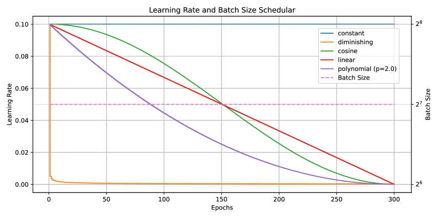
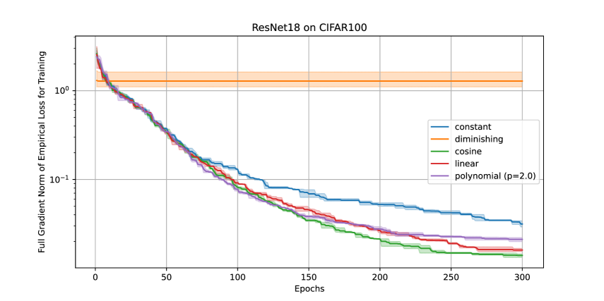
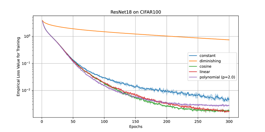
(a) Learning rate $\eta_{t}$ and batch size $b$ versus epochs	(b) Full gradient norm $\|\nabla f(\bm{\theta}_{e})\|$ versus epochs
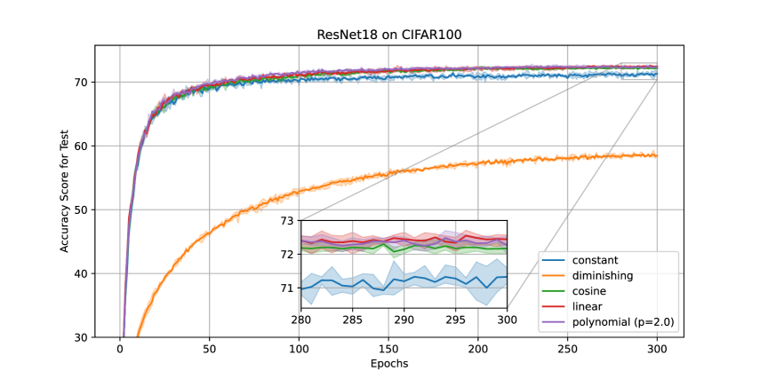
(c) Empirical loss $f(\bm{\theta}_{e})$ versus epochs	(d) Test accuracy score versus epochs

Figure 1: (a) Decaying learning rates (constant, diminishing, cosine, linear, and polynomial) and constant batch size, (b) full gradient norm of empirical loss, (c) empirical loss value, and (d) accuracy score in testing for SGD to train ResNet18 on CIFAR100 dataset.

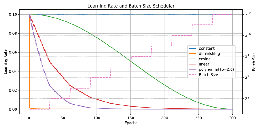
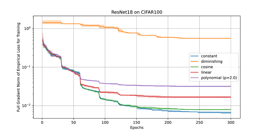
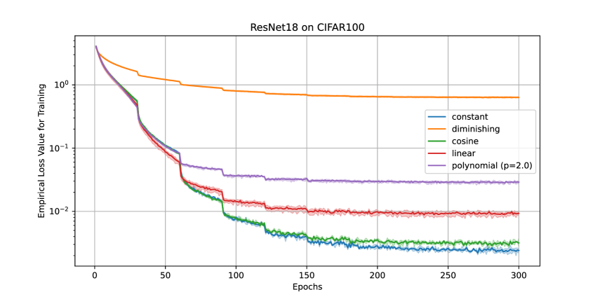
(a) Learning rate $\eta_{t}$ and batch size $b_{t}$ versus epochs	(b) Full gradient norm $\|\nabla f(\bm{\theta}_{e})\|$ versus epochs
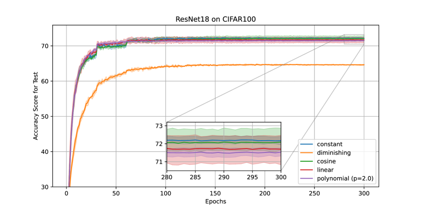
(c) Empirical loss $f(\bm{\theta}_{e})$ versus epochs	(d) Test accuracy score versus epochs

Figure 2: (a) Decaying learning rates and doubly increasing batch size every 30 epochs, (b) full gradient norm of empirical loss, (c) empirical loss value, and (d) accuracy score in testing for SGD to train ResNet18 on CIFAR100 dataset.

We set the total number of epochs $E=300$, the initial learning rate $\eta_{0}=0.1$, and the minimum learning rate $\eta_{\min}=0$ in (4) and (5). The solid line in the figure represents the mean value, and the shaded area in the figure represents the maximum and minimum over three runs.

Let us first consider the case (Figure 1(a)) of a constant batch size ($b=2^{7}$) and decaying learning rates $\eta_{t}$ defined by (2)–(5) discussed in Section 3.1, where “linear" in Figure 1 denotes Polynomial LR (5) with $p=1$. Figure 1(b)–(d) indicate that using Diminishing LR (3) did not work well, since it decayed rapidly and was very small (Figure 1(a)). Figure 1(b)–(d) also indicate that Cosine LR (4) and Polynomial LR (5) performed better than Constant LR (2), as promised in the theoretical results in Theorem 3.1 and (7).

Next, let us consider the case (Figure 2(a)) of doubly increasing batch size every $30$ epochs from an initial batch size $b_{0}=2^{3}$ and decaying learning rates $\eta_{t}$ defined by (2)–(5). Figure 2(a) indicates that the learning rate of Polynomial LR (5) updated each step (“linear" and “polynomial ($p=2.0$)") becomes small at an early stage of training. This is because the smaller the batch size $b_{t}$ is, the larger the required number of steps $K_{t}=\lceil\frac{n}{b_{t}}\rceil$ per epoch becomes and the smaller the decaying learning rate $\eta_{t}$ becomes. Hence, in practice, increasing batch size is not compatible with Polynomial LR (5) updated each step. Meanwhile, Figure 2(a) indicates Constant LR (2) (“constant") and Cosine LR (4) (“cosine") were compatible with increasing batch size, since Constant LR (2) and Cosine LR (4) updated each epoch maintain large learning rates even for small batch sizes. In particular, Figure 2(b)–(d) indicate that using Constant LR (2) performed well.

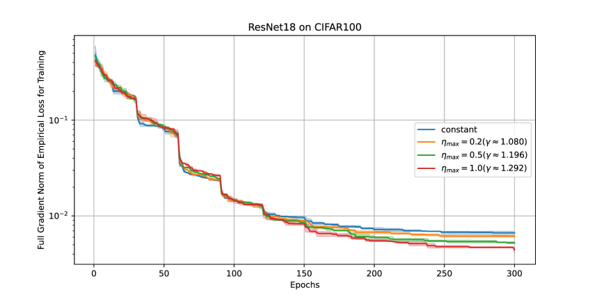
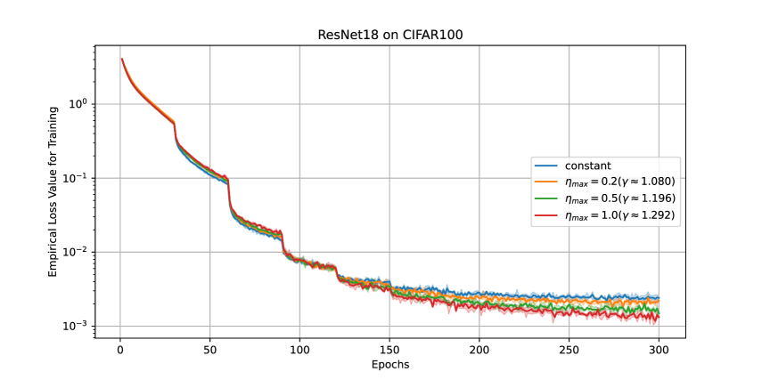
(a) Learning rate $\eta_{t}$ and batch size $b_{t}$ versus epochs	(b) Full gradient norm $\|\nabla f(\bm{\theta}_{e})\|$ versus epochs
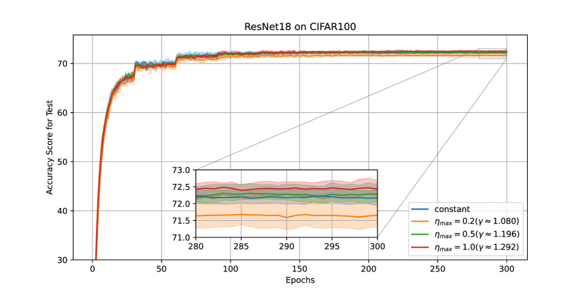
(c) Empirical loss $f(\bm{\theta}_{e})$ versus epochs	(d) Test accuracy score versus epochs

Figure 3: (a) Increasing learning rates ($\eta_{\max}=0.2,0.5,1.0$) and doubly increasing batch size every 30 epochs, (b) full gradient norm of empirical loss, (c) empirical loss value, and (d) accuracy score in testing for SGD to train ResNet18 on CIFAR100 dataset.

Let us consider the case (Figure 3(a)) of doubly increasing batch size ($\delta=2$) every $30$ epochs and increasing learning rates defined by Exponential growth LR (12) with $\eta_{0}=0.1$ . The parameters $\gamma$ in the increasing learning rates considered here were (i) $\gamma\approx 1.080$ when $\eta_{\max}=0.2$, (ii) $\gamma\approx 1.196$ when $\eta_{\max}=0.5$, and (iii) $\gamma\approx 1.292$ when $\eta_{\max}=1.0$, which satisfy the condition $\gamma^{2}<\delta$ ($=2$) to guarantee the convergence of Algorithm 1 (see Theorem 3.3). Figure 3 compares the result for “constant" in Figure 2 with the ones for the increasing learning rates (i)–(iii). Figure 3(b) indicates that the larger the learning rate $\eta_{t}$ was, the smaller the full gradient norm $\|\nabla f(\bm{\theta}_{e})\|$ became and that Algorithm 1 with increasing learning rates minimized the full gradient norm faster than Algorithm 1 with a constant learning rate (“constant" in Figures 2 and 3), as promised in Theorem 3.3.

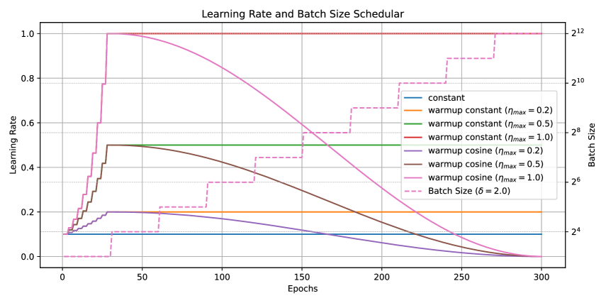
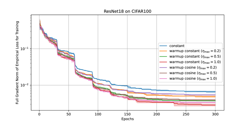
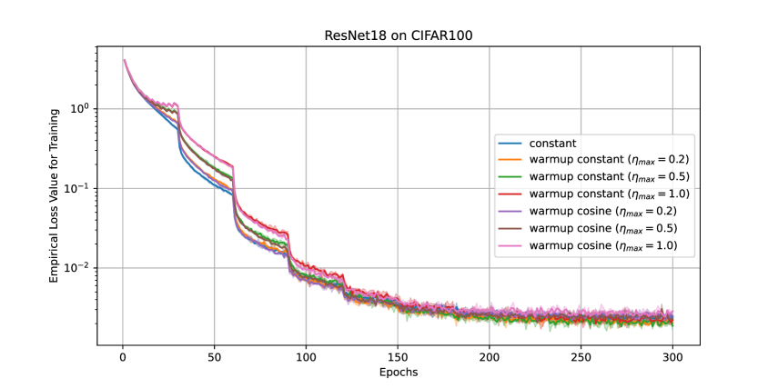
(a) Learning rate $\eta_{t}$ and batch size $b_{t}$ versus epochs	(b) Full gradient norm $\|\nabla f(\bm{\theta}_{e})\|$ versus epochs
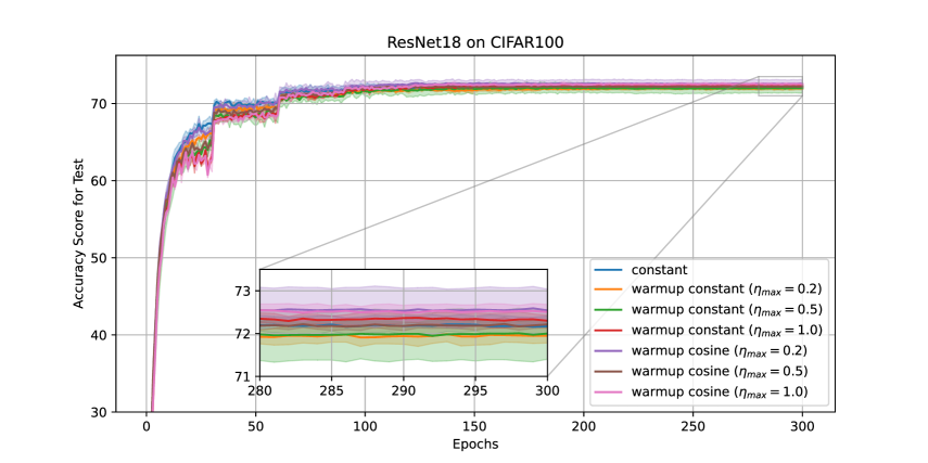
(c) Empirical loss $f(\bm{\theta}_{e})$ versus epochs	(d) Test accuracy score versus epochs

Figure 4: (a) Warm-up learning rates and doubly increasing batch size every 30 epochs, (b) full gradient norm of empirical loss, (c) empirical loss value, and (d) accuracy score in testing for SGD to train ResNet18 on CIFAR100 dataset.

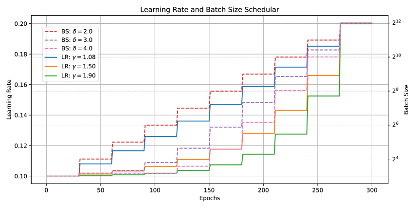
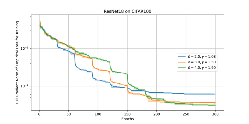
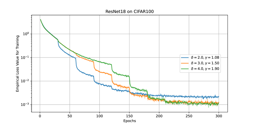
(a) Learning rate $\eta_{t}$ and batch size $b_{t}$ versus epochs	(b) Full gradient norm $\|\nabla f(\bm{\theta}_{e})\|$ versus epochs
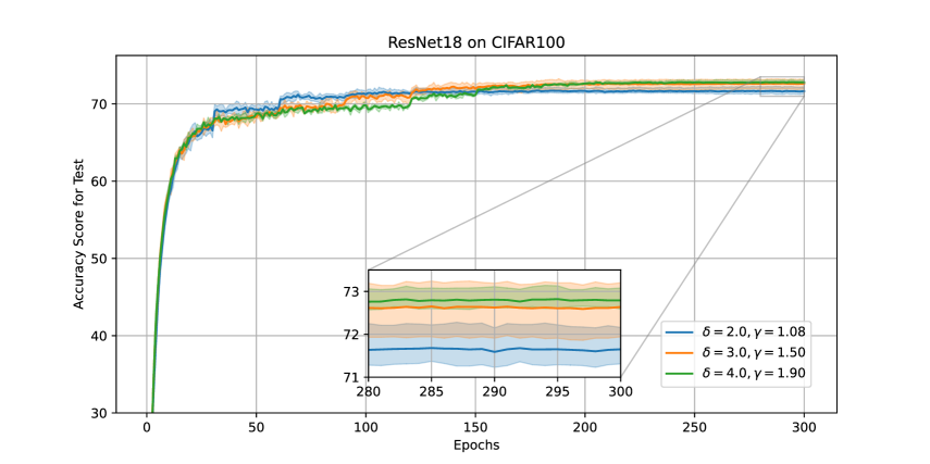
(c) Empirical loss $f(\bm{\theta}_{e})$ versus epochs	(d) Test accuracy score versus epochs

Figure 5: (a) Increasing learning rates and increasing batch sizes based on $\delta=2,3,4$, (b) full gradient norm of empirical loss, (c) empirical loss value, and (d) accuracy score in testing for SGD to train ResNet18 on CIFAR100 dataset.

Let us consider the case (Figure 4(a)) of a doubly increasing batch size and decaying learning rates (Constant LR (2) and Cosine LR (4)) with warm-up based on Figure 3(a). Figure 4(b) indicates that using decaying learning rates with warm-up accelerated Algorithm 1 more than using only increasing learning rates in Figure 3(b) and only a constant learning rate in Figure 2(b).

From the sufficient condition $\gamma^{2}<\delta$ to guarantee convergence of Algorithm 1 with both batch size and learning rate increasing (Theorem 3.3), we can set a larger $\gamma$ when $\delta$ is large. Since Algorithm 1 has an $O(\gamma^{-\frac{M}{2}})$ convergence rate (Theorem 3.3), using triply ($\gamma=1.5<\sqrt{\delta}=\sqrt{3}$) and quadruply ($\gamma=1.9<\sqrt{\delta}=\sqrt{4}$) increasing batch sizes theoretically decreases $\|\nabla f(\bm{\theta}_{e})\|$ faster than doubly increasing batch sizes ($\gamma=1.080<\sqrt{\delta}=\sqrt{2}$ when $\eta_{\max}=0.2$; Figure 3). Finally, we would like to verify whether the theoretical result holds in practice. The scheduler was as in Figure 5(a) with $\eta_{0}=0.1$ and $\eta_{\max}=0.2$, where schedulers were modified such that batch sizes belong to $[2^{3},2^{12}]$ and learning rates belong to $[0.1,0.2]$ (e.g., $b_{e}=a\delta^{\lfloor\frac{e}{30}\rfloor}+b$ and $\eta_{e}=c\gamma^{\lfloor\frac{e}{30}\rfloor}+d$, where $a\approx 0.2077$, $b\approx 7.7923$, $c\approx 0.00267$, and $d\approx 0.09733$ when $\delta=3$ and $\gamma=1.50$ and $a\approx 0.0155$, $b\approx 7.9844$, $c\approx 0.00031$, and $d\approx 0.09969$ when $\delta=4$ and $\gamma=1.90$). Figure 5(a) and (b) indicate that the larger the increasing rate of batch size was (the cases of $\delta=3,4$ after $180$ epochs), the larger the increasing rate of the learning rate became ($\gamma=1.5,1.9$ when $\delta=3,4$) and the smaller $\|\nabla f(\bm{\theta}_{e})\|$ became. That is, using increasing learning rates based on tripling and quadrupling batch sizes minimizes $\|\nabla f(\bm{\theta}_{e})\|$ faster than using increasing learning rates based on doubly increasing batch sizes. Figure 5(c) and (d) indicate that using $\delta=3,4$ was better than using $\delta=2$ in the sense of minimizing $f(\bm{\theta}_{e})$ and achieving high test accuracy.

5 Conclusion

This paper presented theoretical analyses of mini-batch SGD under batch size and learning rate schedulers used in practice. Our results indicated that using increasing batch sizes and decaying learning rates guarantees convergence of mini-batch SGD and using both batch sizes and learning rates that increase accelerates mini-batch SGD. That is, using increasing batch sizes and decaying learning rates with warm-up guarantees fast convergence of mini-batch SGD in the sense of minimizing the expectation of the full gradient norm of the empirical loss. This paper also provided numerical results to support the analysis results that increasing both batch sizes and learning rates accelerates mini-batch SGD. One limitation of this study is that the numbers of models and datasets in the experiments were limited. Hence, we should conduct similar experiments with larger numbers of models and datasets to support our theoretical results.

Appendix A Appendix

We here give the notation and state some definitions. Let $\mathbb{N}$ be the set of natural numbers. Define $[n]:=\{1,2,\cdots,n\}$ and $[0:n]:=\{0,1,\cdots,n\}$ for $n\in\mathbb{N}$. Let $\mathbb{R}^{d}$ be the $d$-dimensional Euclidean space with inner product $\langle\bm{\theta}_{1},\bm{\theta}_{2}\rangle=\bm{\theta}_{1}^{\top}\bm{\theta}_{2}$ $(\bm{\theta}_{1},\bm{\theta}_{2}\in\mathbb{R}^{d})$ and its induced norm $\|\bm{\theta}\|:=\sqrt{\langle\bm{\theta},\bm{\theta}\rangle}$ $(\bm{\theta}\in\mathbb{R}^{d})$. Let $\mathbb{R}_{+}^{d}:=\{\bm{\theta}=(\theta_{1},\theta_{2},\ldots,\theta_{d})^{\top}\in\mathbb{R}^{d}\colon\theta_{i}\geq 0\text{ }(i\in[d])\}$ and $\mathbb{R}_{++}^{d}:=\{\bm{\theta}=(\theta_{1},\theta_{2},\ldots,\theta_{d})^{\top}\in\mathbb{R}^{d}\colon\theta_{i}>0\text{ }(i\in[d])\}$. The gradient of a differentiable function $f\colon\mathbb{R}^{d}\to\mathbb{R}$ at $\bm{\theta}\in\mathbb{R}^{d}$ is denoted by $\nabla f(\bm{\theta})$. Let $L>0$. A differentiable function $f\colon\mathbb{R}^{d}\to\mathbb{R}$ is said to be $L$-smooth if the gradient $\nabla f\colon\mathbb{R}^{d}\to\mathbb{R}^{d}$ is Lipschitz continuous, i.e., for all $\bm{\theta}_{1},\bm{\theta}_{2}\in\mathbb{R}^{d}$, $\|\nabla f(\bm{\theta}_{1})-\nabla f(\bm{\theta}_{2})\|\leq L\|\bm{\theta}_{1}-\bm{\theta}_{2}\|$. Let $(x_{t}),(y_{t})\subset\mathbb{R}_{+}$ be sequences. Let $O$ be Landau’s symbol, i.e., $y_{t}=O(x_{t})$ if there exist $c\in\mathbb{R}_{+}$ and $t_{0}\in\mathbb{N}$ such that, for all $t\geq t_{0}$, $y_{t}\leq cx_{t}$.

A.1 Proofs of Proposition A.1 and Lemma 2.1

The following proposition holds for the mini-batch gradient.

Proposition A.1.

Let $t\in\mathbb{N}$ and $\bm{\xi}_{t}$ be a random variable that is independent of $\bm{\xi}_{j}$ ($j\in[0:t-1]$); let $\bm{\theta}_{t}\in\mathbb{R}^{d}$ be independent of $\bm{\xi}_{t}$; let $\nabla f_{B_{t}}(\bm{\theta}_{t})$ be the mini-batch gradient defined by Algorithm 1, where $f_{\xi_{t,i}}$ ($i\in[b]$) is the stochastic gradient (see Assumption 2.1(A2)). Then, the following hold:

$$\mathbb{E}_{\bm{\xi}_{t}}\left[\nabla f_{B_{t}}(\bm{\theta}_{t})\Big{|}\hat{\bm{\xi}}_{t-1}\right]=\nabla f(\bm{\theta}_{t})\text{ and }\mathbb{V}_{\bm{\xi}_{t}}\left[\nabla f_{B_{t}}(\bm{\theta}_{t})\Big{|}\hat{\bm{\xi}}_{t-1}\right]\leq\frac{\sigma^{2}}{b_{t}},$$

where $\mathbb{E}_{\bm{\xi}_{t}}[\cdot|\hat{\bm{\xi}}_{t-1}]$ and $\mathbb{V}_{\bm{\xi}_{t}}[\cdot|\hat{\bm{\xi}}_{t-1}]$ are respectively the expectation and variance with respect to $\bm{\xi}_{t}$ conditioned on $\bm{\xi}_{t-1}=\hat{\bm{\xi}}_{t-1}$.

The first equation in Proposition A.1 indicates that the mini-batch gradient $\nabla f_{B_{t}}(\bm{\theta}_{t})$ is an unbiased estimator of the full gradient $\nabla f(\bm{\theta}_{t})$. The second inequality in Proposition A.1 indicates that the upper bound on the variance of the mini-batch gradient $\nabla f_{B_{t}}(\bm{\theta}_{t})$ is inversely proportional to the batch size $b_{t}$.

Proof of Proposition A.1: Assumption 2.1(A3) and the independence of $b_{t}$ and $\bm{\xi}_{t}$ ensure that

$$\mathbb{E}_{\bm{\xi}_{t}}\left[\nabla f_{B_{t}}(\bm{\theta}_{t})\Big{|}\hat{\bm{\xi}}_{t-1}\right]=\mathbb{E}_{\bm{\xi}_{t}}\left[\frac{1}{b_{t}}\sum_{i=1}^{b_{t}}\nabla f_{\xi_{t,i}}(\bm{\theta}_{t})\Bigg{|}\hat{\bm{\xi}}_{t-1}\right]=\frac{1}{b_{t}}\sum_{i=1}^{b_{t}}\mathbb{E}_{\xi_{t,i}}\left[\nabla f_{\xi_{t,i}}(\bm{\theta}_{t})\Big{|}\hat{\bm{\xi}}_{t-1}\right],$$

which, together with Assumption 2.1(A2)(i) and the independence of $\bm{\xi}_{t}$ and $\bm{\xi}_{t-1}$, implies that

$$\mathbb{E}_{\bm{\xi}_{t}}\left[\nabla f_{B_{t}}(\bm{\theta}_{t})\Big{|}\hat{\bm{\xi}}_{t-1}\right]=\frac{1}{b_{t}}\sum_{i=1}^{b_{t}}\nabla f(\bm{\theta}_{t})=\nabla f(\bm{\theta}_{t}).$$ (16)

Assumption 2.1(A3), the independence of $b_{t}$ and $\bm{\xi}_{t}$, and (16) imply that

$$\mathbb{V}_{\bm{\xi}_{t}}\left[\nabla f_{B_{t}}(\bm{\theta}_{t})\Big{|}\hat{\bm{\xi}}_{t-1}\right] =\mathbb{E}_{\bm{\xi}_{t}}\left[\|\nabla f_{B_{t}}(\bm{\theta}_{t})-\nabla f(\bm{\theta}_{t})\|^{2}\Big{|}\hat{\bm{\xi}}_{t-1}\right]$$

$$=\mathbb{E}_{\bm{\xi}_{t}}\left[\left\|\frac{1}{b_{t}}\sum_{i=1}^{b_{t}}\nabla f_{\xi_{t,i}}(\bm{\theta}_{t})-\nabla f(\bm{\theta}_{t})\right\|^{2}\Bigg{|}\hat{\bm{\xi}}_{t-1}\right]$$

$$=\frac{1}{b_{t}^{2}}\mathbb{E}_{\bm{\xi}_{t}}\left[\left\|\sum_{i=1}^{b_{t}}\left(\nabla f_{\xi_{t,i}}(\bm{\theta}_{t})-\nabla f(\bm{\theta}_{t})\right)\right\|^{2}\Bigg{|}\hat{\bm{\xi}}_{t-1}\right].$$

From the independence of $\xi_{t,i}$ and $\xi_{t,j}$ ($i\neq j$) and Assumption 2.1(A2)(i), for all $i,j\in[b_{t}]$ such that $i\neq j$,

$$\mathbb{E}_{\xi_{t,i}}[\langle\nabla f_{\xi_{t,i}}(\bm{\theta}_{t})-\nabla f(\bm{\theta}_{t}),\nabla f_{\xi_{t,j}}(\bm{\theta}_{t})-\nabla f(\bm{\theta}_{t})\rangle|\hat{\bm{\xi}}_{t-1}]$$

$$=\langle\mathbb{E}_{\xi_{t,i}}[\nabla f_{\xi_{t,i}}(\bm{\theta}_{t})|\hat{\bm{\xi}}_{t-1}]-\mathbb{E}_{\xi_{t,i}}[\nabla f(\bm{\theta}_{t})|\hat{\bm{\xi}}_{t-1}],\nabla f_{\xi_{t,j}}(\bm{\theta}_{t})-\nabla f(\bm{\theta}_{t})\rangle$$

$$=0.$$

Hence, Assumption 2.1(A2)(ii) guarantees that

$$\mathbb{V}_{\bm{\xi}_{t}}\left[\nabla f_{B_{t}}(\bm{\theta})\Big{|}\hat{\bm{\xi}}_{t-1}\right]=\frac{1}{b_{t}^{2}}\sum_{i=1}^{b_{t}}\mathbb{E}_{\xi_{t,i}}\left[\left\|\nabla f_{\xi_{t,i}}(\bm{\theta}_{t})-\nabla f(\bm{\theta}_{t})\right\|^{2}\Big{|}\hat{\bm{\xi}}_{t-1}\right]\leq\frac{\sigma^{2}b_{t}}{b_{t}^{2}}=\frac{\sigma^{2}}{b_{t}},$$

which completes the proof. $\Box$

Proof of Lemma 2.1: The $L_{n}$-smoothness of $f$ implies that the descent lemma holds; i.e., for all $t\in\mathbb{N}$,

$$f(\bm{\theta}_{t+1})\leq f(\bm{\theta}_{t})+\langle\nabla f(\bm{\theta}_{t}),\bm{\theta}_{t+1}-\bm{\theta}_{t}\rangle+\frac{L_{n}}{2}\|\bm{\theta}_{t+1}-\bm{\theta}_{t}\|^{2},$$

which, together with $\bm{\theta}_{t+1}:=\bm{\theta}_{t}-\eta_{t}\nabla f_{B_{t}}(\bm{\theta}_{t})$, implies that

$$\begin{split}f(\bm{\theta}_{t+1})&\leq f(\bm{\theta}_{t})-\eta_{t}\langle\nabla f(\bm{\theta}_{t}),\nabla f_{B_{t}}(\bm{\theta}_{t})\rangle+\frac{L_{n}\eta_{t}^{2}}{2}\|\nabla f_{B_{t}}(\bm{\theta}_{t})\|^{2}.\end{split}$$ (17)

Proposition A.1 guarantees that

$$\begin{split}\mathbb{E}_{\bm{\xi}_{t}}\left[\left\|\nabla f_{B_{t}}(\bm{\theta}_{t})\right\|^{2}|\hat{\bm{\xi}}_{t-1}\right]&=\mathbb{E}_{\bm{\xi}_{t}}\left[\left\|\nabla f_{B_{t}}(\bm{\theta}_{t})-\nabla f(\bm{\theta}_{t})+\nabla f(\bm{\theta}_{t})\right\|^{2}\Big{|}\hat{\bm{\xi}}_{t-1}\right]\\ &=\mathbb{E}_{\bm{\xi}_{t}}\left[\left\|\nabla f_{B_{t}}(\bm{\theta}_{t})-\nabla f(\bm{\theta}_{t})\right\|^{2}\Big{|}\hat{\bm{\xi}}_{t-1}\right]\\ &\quad+2\mathbb{E}_{\bm{\xi}_{t}}\left[\langle\nabla f_{B_{t}}(\bm{\theta}_{t})-\nabla f(\bm{\theta}_{t}),\nabla f(\bm{\theta}_{t})\rangle\Big{|}\hat{\bm{\xi}}_{t-1}\right]\\ &\quad+\mathbb{E}_{\bm{\xi}_{t}}\left[\left\|\nabla f(\bm{\theta}_{t})\right\|^{2}\Big{|}\hat{\bm{\xi}}_{t-1}\right]\\ &\leq\frac{\sigma^{2}}{b_{t}}+\left\|\nabla f(\bm{\theta}_{t})\right\|^{2}.\end{split}$$ (18)

Taking the expectation conditioned on $\bm{\xi}_{t-1}=\hat{\bm{\xi}}_{t-1}$ on both sides of (17), together with Proposition A.1 and (18), guarantees that, for all $k\in\mathbb{N}$,

$$\mathbb{E}_{\bm{\xi}_{t}}\left[f(\bm{\theta}_{t+1})\Big{|}\hat{\bm{\xi}}_{t-1}\right] \leq f(\bm{\theta}_{t})-\eta_{t}\mathbb{E}_{\bm{\xi}_{t}}\left[\langle\nabla f(\bm{\theta}_{t}),\nabla f_{B_{t}}(\bm{\theta}_{t})\rangle\Big{|}\hat{\bm{\xi}}_{t-1}\right]$$

$$\quad+\frac{L_{n}\eta_{t}^{2}}{2}\mathbb{E}_{\bm{\xi}_{t}}\left[\left\|\nabla f_{B_{t}}(\bm{\theta}_{t})\right\|^{2}\Big{|}\hat{\bm{\xi}}_{t-1}\right]$$

$$\leq f(\bm{\theta}_{t})-\eta_{t}\left\|\nabla f(\bm{\theta}_{t})\right\|^{2}+\frac{L_{n}\eta_{t}^{2}}{2}\left(\frac{\sigma^{2}}{b_{t}}+\left\|\nabla f(\bm{\theta}_{t})\right\|^{2}\right).$$

Hence, taking the total expectation on both sides of the above inequality ensures that, for all $t\in\mathbb{N}$,

$$\eta_{k}\left(1-\frac{L_{n}\eta_{t}}{2}\right)\mathbb{E}\left[\left\|\nabla f(\bm{\theta}_{t})\right\|^{2}\right]\leq\mathbb{E}\left[f(\bm{\theta}_{t})-f(\bm{\theta}_{t+1})\right]+\frac{L_{n}\sigma^{2}\eta_{t}^{2}}{2b_{t}}.$$

Let $T\in\mathbb{N}$. Summing the above inequality from $t=0$ to $t=T-1$ ensures that

$$\sum_{t=0}^{T-1}\eta_{t}\left(1-\frac{L_{n}\eta_{t}}{2}\right)\mathbb{E}\left[\left\|\nabla f(\bm{\theta}_{t})\right\|^{2}\right]\leq\mathbb{E}\left[f(\bm{\theta}_{0})-f(\bm{\theta}_{T})\right]+\frac{L_{n}\sigma^{2}}{2}\sum_{t=0}^{T-1}\frac{\eta_{t}^{2}}{b_{t}},$$

which, together with Assumption 2.1(A1) (the lower bound $f^{\star}:=\frac{1}{n}\sum_{i\in[n]}f_{i}^{\star}$ of $f$), implies that

$$\sum_{t=0}^{T-1}\eta_{t}\left(1-\frac{L_{n}\eta_{t}}{2}\right)\mathbb{E}\left[\left\|\nabla f(\bm{\theta}_{t})\right\|^{2}\right]\leq f(\bm{\theta}_{0})-f^{\star}+\frac{L_{n}\sigma^{2}}{2}\sum_{t=0}^{T-1}\frac{\eta_{t}^{2}}{b_{t}}.$$

Since $\eta_{t}\in[\eta_{\min},\eta_{\max}]$, we have that

$$\left(1-\frac{L_{n}\eta_{\max}}{2}\right)\sum_{t=0}^{T-1}\eta_{t}\mathbb{E}\left[\left\|\nabla f(\bm{\theta}_{t})\right\|^{2}\right]\leq f(\bm{\theta}_{0})-f^{\star}+\frac{L_{n}\sigma^{2}}{2}\sum_{t=0}^{T-1}\frac{\eta_{t}^{2}}{b_{t}},$$

which, together with $\eta_{t}\in[\eta_{\min},\eta_{\max}]\subset[0,\frac{2}{L_{n}})$, implies that

$$\sum_{t=0}^{T-1}\eta_{t}\mathbb{E}\left[\left\|\nabla f(\bm{\theta}_{t})\right\|^{2}\right]\leq\frac{2(f(\bm{\theta}_{0})-f^{\star})}{2-L_{n}\eta_{\max}}+\frac{L_{n}\sigma^{2}}{2-L_{n}\eta_{\max}}\sum_{t=0}^{T-1}\frac{\eta_{t}^{2}}{b_{t}}.$$

Therefore, from $\sum_{t=0}^{T-1}\eta_{t}\neq 0$, we have

$$\min_{t\in[0:T-1]}\mathbb{E}[\|\nabla f(\bm{\theta}_{t})\|^{2}]\leq\frac{2(f(\bm{\theta}_{0})-f^{\star})}{2-L_{n}\eta_{\max}}\frac{1}{\sum_{t=0}^{T-1}\eta_{t}}+\frac{L_{n}\sigma^{2}}{2-L_{n}\eta_{\max}}\frac{\sum_{t=0}^{T-1}\eta_{t}^{2}b_{t}^{-1}}{\sum_{t=0}^{T-1}\eta_{t}},$$ (19)

which implies that the assertion in Lemma 2.1 holds. $\Box$

A.2 Proofs of Theorems

We can also consider the case where batch sizes decay. For simplicity, let us set a constant learning rate $\eta_{t}=\eta>0$ and a decaying batch size $b_{t}=\frac{1}{t+1}$. Then, we have that $V_{T}\leq\frac{\eta}{T}\sum_{t=0}^{T-1}\frac{1}{b_{t}}=\frac{\eta(T+1)}{2}\to+\infty$ ($T\to+\infty$), which implies that convergence of mini-batch SGD is not guaranteed. Accordingly, this paper focuses on the four cases in the main text.

Proof of Theorem 3.1: Let $\eta_{\max}=\eta$.

[Constant LR (2)] We have that

$$B_{T}=\frac{1}{\sum_{t=0}^{T-1}\eta}=\frac{1}{\eta T},\text{ }V_{T}=\frac{\sum_{t=0}^{T-1}\eta^{2}}{b\sum_{t=0}^{T-1}\eta}=\frac{\eta}{b}.$$

[Diminishing LR (3)] We have that

$$\sum_{t=0}^{T-1}\frac{1}{\sqrt{t+1}}\geq\int_{0}^{T}\frac{\mathrm{d}t}{\sqrt{t+1}}=2(\sqrt{T+1}-1),$$

which implies that

$$B_{T}=\frac{1}{\sum_{t=0}^{T-1}\frac{\eta}{\sqrt{t+1}}}\leq\frac{1}{2\eta(\sqrt{T+1}-1)}.$$

We also have that

$$\sum_{t=0}^{T-1}\frac{1}{t+1}\leq 1+\int_{0}^{T-1}\frac{\mathrm{d}t}{t+1}=1+\log T,$$

which implies that

$$V_{T}=\frac{\eta\sum_{t=0}^{T-1}\frac{1}{t+1}}{b\sum_{t=0}^{T-1}\frac{1}{\sqrt{t+1}}}\leq\frac{\eta(1+\log T)}{2b(\sqrt{T+1}-1)}.$$

[Cosine LR (4)] We have

$$\sum_{t=0}^{KE-1}\eta_{t} =\eta_{\min}KE+\frac{\eta_{\max}-\eta_{\min}}{2}KE+\frac{\eta_{\max}-\eta_{\min}}{2}\sum_{t=0}^{KE-1}\cos\left\lfloor\frac{t}{K}\right\rfloor\frac{\pi}{E}.$$

From $\sum_{t=0}^{KE}\cos\lfloor\frac{t}{K}\rfloor\frac{\pi}{E}=K-1$, we have

$$\sum_{t=0}^{KE-1}\cos\left\lfloor\frac{t}{K}\right\rfloor\frac{\pi}{E}=K-1-\cos\pi=K.$$ (20)

We thus have

$$\sum_{t=0}^{KE-1}\eta_{t} =\eta_{\min}KE+\frac{\eta_{\max}-\eta_{\min}}{2}KE+\frac{\eta_{\max}-\eta_{\min}}{2}K$$

$$=\frac{1}{2}\{(\eta_{\min}+\eta_{\max})KE+(\eta_{\max}-\eta_{\min})K\}$$

$$\geq\frac{(\eta_{\min}+\eta_{\max})KE}{2}.$$

Moreover, we have that

$$\sum_{t=0}^{KE-1}\eta_{t}^{2} =\eta_{\min}^{2}KE+\eta_{\min}(\eta_{\max}-\eta_{\min})\sum_{t=0}^{KE-1}\left(1+\cos\left\lfloor\frac{t}{K}\right\rfloor\frac{\pi}{E}\right)$$

$$\quad+\frac{(\eta_{\max}-\eta_{\min})^{2}}{4}\sum_{t=0}^{KE-1}\left(1+\cos\left\lfloor\frac{t}{K}\right\rfloor\frac{\pi}{E}\right)^{2},$$

which implies that

$$\sum_{t=0}^{KE-1}\eta_{t}^{2} =\eta_{\min}\eta_{\max}KE+\frac{(\eta_{\max}-\eta_{\min})^{2}}{4}KE+\eta_{\min}(\eta_{\max}-\eta_{\min})\sum_{t=0}^{KE-1}\cos\left\lfloor\frac{t}{K}\right\rfloor\frac{\pi}{E}$$

$$\quad+\frac{(\eta_{\max}-\eta_{\min})^{2}}{2}\sum_{t=0}^{KE-1}\cos\left\lfloor\frac{t}{K}\right\rfloor\frac{\pi}{E}+\frac{(\eta_{\max}-\eta_{\min})^{2}}{4}\sum_{t=0}^{KE-1}\cos^{2}\left\lfloor\frac{t}{K}\right\rfloor\frac{\pi}{E}.$$

From

$$\sum_{t=0}^{KE}\cos^{2}\left\lfloor\frac{t}{K}\right\rfloor\frac{\pi}{E} =\frac{1}{2}\sum_{t=0}^{KE}\left(1+\cos 2\left\lfloor\frac{t}{K}\right\rfloor\frac{\pi}{E}\right)$$

$$=\frac{1}{2}(KE+1)+\frac{1}{2}$$

$$=\frac{KE}{2}+1,$$

we have

$$\sum_{t=0}^{KE-1}\cos^{2}\left\lfloor\frac{t}{K}\right\rfloor\frac{\pi}{E}=\frac{KE}{2}+1-\cos^{2}\pi=\frac{KE}{2}.$$

From (20), we have

$$\sum_{t=0}^{KE-1}\eta_{t}^{2} =\frac{(\eta_{\min}+\eta_{\max})^{2}}{4}KE+\eta_{\min}(\eta_{\max}-\eta_{\min})+\frac{(\eta_{\max}-\eta_{\min})^{2}}{2}+\frac{(\eta_{\max}-\eta_{\min})^{2}}{4}\frac{KE}{2}$$

$$=\frac{3\eta_{\min}^{2}+2\eta_{\min}\eta_{\max}+3\eta_{\max}^{2}}{8}KE+\frac{(\eta_{\max}-\eta_{\min})(\eta_{\max}+\eta_{\min})}{2}.$$

Hence, we have

$$B_{T}=\frac{1}{\sum_{t=0}^{KE-1}\eta_{t}}\leq\frac{2}{(\eta_{\min}+\eta_{\max})KE}$$

and

$$V_{T}=\frac{\sum_{t=0}^{KE-1}\eta_{t}^{2}}{b\sum_{t=0}^{KE-1}\eta_{t}} \leq\frac{3\eta_{\min}^{2}+2\eta_{\min}\eta_{\max}+3\eta_{\max}^{2}}{4(\eta_{\min}+\eta_{\max})b}+\frac{\eta_{\max}-\eta_{\min}}{bKE}.$$

[Polynomial LR (5)] Since $f(x)=(1-x)^{p}$ is monotone decreasing for $x\in[0,1)$, we have that

$$\int_{0}^{1}(1-x)^{p}\mathrm{d}x<\frac{1}{T}\sum_{t=0}^{T-1}\left(1-\frac{t}{T}\right)^{p},$$

which implies that

$$T\int_{0}^{1}(1-x)^{p}dx<\sum_{t=0}^{T-1}\left(1-\frac{t}{T}\right)^{p}.$$ (21)

Since $\int_{0}^{1}(1-x)^{p}\mathrm{d}x=\frac{1}{p+1}$, (21) implies that

$$\sum_{t=0}^{T-1}\left(1-\frac{t}{T}\right)^{p}>\frac{T}{p+1}.$$

Accordingly,

$$\sum_{t=0}^{T-1}\eta_{t} =(\eta_{\max}-\eta_{\min})\sum_{t=0}^{T-1}\left(1-\frac{t}{T}\right)^{p}+\eta_{\min}T$$

$$>(\eta_{\max}-\eta_{\min})\frac{T}{p+1}+\eta_{\min}T$$

$$=\left(\frac{\eta_{\max}-\eta_{\min}}{p+1}+\eta_{\min}\right)T$$

$$=\frac{\eta_{\max}+\eta_{\min}p}{p+1}T.$$

Since $f(x)=(1-x)^{p}$ and $g(x)=(1-x)^{2p}$ are monotone decreasing for $x\in[0,1)$, we have that

$$\frac{1}{T}\sum_{t=0}^{T-1}\left(1-\frac{t}{T}\right)^{p}<\frac{1}{T}+\int_{0}^{1}(1-x)^{p}\mathrm{d}x,\text{ }\frac{1}{T}\sum_{t=0}^{T-1}\left(1-\frac{t}{T}\right)^{2p}<\frac{1}{T}+\int_{0}^{1}(1-x)^{2p}\mathrm{d}x,$$

which imply that

$$\sum_{t=0}^{T-1}\left(1-\frac{t}{T}\right)^{p}<1+T\int_{0}^{1}(1-x)^{p}\mathrm{d}x,\text{ }\sum_{t=0}^{T-1}\left(1-\frac{t}{T}\right)^{2p}<1+T\int_{0}^{1}(1-x)^{2p}\mathrm{d}x.$$ (22)

Since we have that $\int_{0}^{1}(1-x)^{p}\mathrm{d}x=\frac{1}{p+1}$ and $\int_{0}^{1}(1-x)^{2p}\mathrm{d}x=\frac{1}{2p+1}$, (22) ensures that

$$\sum_{t=0}^{T-1}\left(1-\frac{t}{T}\right)^{p}<1+\frac{T}{p+1},\text{ }\sum_{t=0}^{T-1}\left(1-\frac{t}{T}\right)^{2p}<1+\frac{T}{2p+1}.$$

Hence,

$$\sum_{t=0}^{T-1}\eta_{t}^{2} =(\eta_{\max}-\eta_{\min})^{2}\sum_{t=0}^{T-1}\left(1-\frac{t}{T}\right)^{2p}+2(\eta_{\max}-\eta_{\min})\sum_{t=0}^{T-1}\left(1-\frac{t}{T}\right)^{p}\eta_{\min}+\eta_{\min}^{2}T$$

$$<(\eta_{\max}-\eta_{\min})^{2}\left(1+\frac{T}{2p+1}\right)+2(\eta_{\max}-\eta_{\min})\left(1+\frac{T}{p+1}\right)\eta_{\min}+\eta_{\min}^{2}T$$

$$=\frac{\eta_{\max}^{2}(p+1)(2p+T+1)+2\eta_{\max}\eta_{\min}pT+\eta_{\min}^{2}(2p^{2}(T-1)-3p-1)}{(p+1)(2p+1)}.$$

Therefore,

$$B_{T}=\frac{1}{\sum_{t=0}^{T-1}\eta_{t}}\leq\frac{p+1}{(\eta_{\max}+\eta_{\min}p)T}$$

and

$$V_{T} =\frac{\sum_{t=0}^{T-1}\eta_{t}^{2}}{b\sum_{t=0}^{T-1}\eta_{t}}$$

$$=\frac{\eta_{\max}^{2}(p+1)(2p+T+1)+2\eta_{\max}\eta_{\min}pT+\eta_{\min}^{2}(2p^{2}(T-1)-3p-1)}{(2p+1)(\eta_{\max}+\eta_{\min}p)bT}$$

$$=\frac{2p^{2}\eta_{\min}^{2}+2p\eta_{\min}\eta_{\max}+(p+1)\eta_{\max}^{2}}{(2p+1)(p\eta_{\min}+\eta_{\max})b}+\frac{(p+1)(2p+1)\eta_{\max}^{2}-(p+1)(2p+1)\eta_{\min}^{2}}{(2p+1)(p\eta_{\min}+\eta_{\max})bT}$$

$$=\frac{2p^{2}\eta_{\min}^{2}+2p\eta_{\min}\eta_{\max}+(p+1)\eta_{\max}^{2}}{(2p+1)(p\eta_{\min}+\eta_{\max})b}+\frac{(p+1)(\eta_{\max}^{2}-\eta_{\min}^{2})}{(p\eta_{\min}+\eta_{\max})bT}.$$

This completes the proof. $\Box$

We will now show the following theorem, which includes Theorem 3.2.

Theorem A.1 (Convergence rate of SGD using (8)).

Under the assumptions in Lemma 2.1, Algorithm 1 using (8) satisfies that, for all $M\in\mathbb{N}$,

$$\min_{t\in[0:T-1]}\mathbb{E}\left[\|\nabla f(\bm{\theta}_{t})\|^{2}\right]\leq\frac{2(f(\bm{\theta}_{0})-f^{\star})}{2-L_{n}\eta_{\max}}\underbrace{\frac{1}{\sum_{t=0}^{T-1}\eta_{t}}}_{B_{T}}+\frac{L_{n}\sigma^{2}}{2-L_{n}\eta_{\max}}\underbrace{\frac{1}{\sum_{t=0}^{T-1}\eta_{t}}\sum_{t=0}^{T-1}\frac{\eta_{t}^{2}}{b_{t}}}_{V_{T}},$$

where $T=\sum_{m=0}^{M}K_{m}E_{m}$, $E_{\max}=\sup_{M\in\mathbb{N}}\sup_{m\in[0:M]}E_{m}<+\infty$, $K_{\max}=\sup_{M\in\mathbb{N}}\sup_{m\in[0:M]}K_{m}<+\infty$, $B_{T}$ is defined as in (6), and $V_{T}$ is given by

$$V_{T}\leq\begin{cases}\displaystyle{\frac{3\eta K_{\max}E_{\max}}{a^{c}T}}&\text{ {\em[Constant LR (\ref{constant})]}}\\ \displaystyle{\frac{3\eta K_{\max}E_{\max}}{2a^{c}(\sqrt{T+1}-1)}}&\text{ {\em[Diminishing LR (\ref{diminishing})]}}\\ \displaystyle{\frac{6\eta_{\max}^{2}K_{\max}E_{\max}}{a^{c}(\eta_{\min}+\eta_{\max})T}}&\text{ {\em[Cosine LR (\ref{cosine})]}}\\ \displaystyle{\frac{3(p+1)\eta_{\max}^{2}K_{\max}E_{\max}}{a^{c}(\eta_{\max}+\eta_{\min}p)T}}&\text{ {\em[Polynomial LR (\ref{polynomial})]}}\end{cases}\quad\text{ {\em([Polynomial BS (\ref{polynomial_bs})])}}$$

$$V_{T}\leq\begin{cases}\displaystyle{\frac{\gamma\eta K_{\max}E_{\max}}{(\gamma-1)b_{0}T}}&\text{ {\em[Constant LR (\ref{constant})]}}\\ \displaystyle{\frac{\gamma\eta K_{\max}E_{\max}}{2(\gamma-1)b_{0}(\sqrt{T+1}-1)}}&\text{ {\em[Diminishing LR (\ref{diminishing})]}}\\ \displaystyle{\frac{2\gamma\eta_{\max}^{2}K_{\max}E_{\max}}{(\gamma-1)(\eta_{\min}+\eta_{\max})b_{0}T}}&\text{ {\em[Cosine LR (\ref{cosine})]}}\\ \displaystyle{\frac{(p+1)\gamma\eta_{\max}^{2}K_{\max}E_{\max}}{(\gamma-1)(\eta_{\max}+\eta_{\min}p)b_{0}T}}&\text{ {\em[Polynomial LR (\ref{polynomial})]}}.\end{cases}\text{ {\em([Exponential BS (\ref{exponential_bs})])}}$$

That is, Algorithm 1 using each of Polynomial BS (9) and Exponential BS (10) has the convergence rate

$$\min_{t\in[0:T-1]}\mathbb{E}\left[\|\nabla f(\bm{\theta}_{t})\|\right]=\begin{cases}\displaystyle{O\left(\frac{1}{\sqrt{T}}\right)}&\text{ {\em[Constant LR (\ref{constant}), Cosine LR (\ref{cosine}), Polynomial LR (\ref{polynomial})]}}\\ \displaystyle{O\left(\frac{1}{T^{\frac{1}{4}}}\right)}&\text{ {\em[Diminishing LR (\ref{diminishing})]}}.\end{cases}$$

Proof of Theorem A.1: Let $M\in\mathbb{N}$ and $T=\sum_{m=0}^{M}K_{m}E_{m}$, where $E_{\max}=\sup_{M\in\mathbb{N}}\sup_{m\in[0:M]}E_{m}<+\infty$, $K_{\max}=\sup_{M\in\mathbb{N}}\sup_{m\in[0:M]}K_{m}<+\infty$, $S_{0}:=\mathbb{N}\cap[0,K_{0}E_{0})$, and $S_{m}=\mathbb{N}\cap[\sum_{k=0}^{m-1}K_{k}E_{k},\sum_{k=0}^{m}K_{k}E_{k})$ ($m\in[M]$). Let us consider using (9).

[Constant LR (2)] Let $m\in[M]$. We have that

$$\sum_{t\in S_{m}}\frac{1}{b_{t}} =\sum_{t\in S_{m}}\frac{1}{\left(am\left\lceil\frac{t}{\sum_{k=0}^{m}K_{k}E_{k}}\right\rceil+b_{0}\right)^{c}}\leq\sum_{t\in S_{m}}\frac{1}{a^{c}m^{c}\left\lceil\frac{t}{\sum_{k=0}^{m}K_{k}E_{k}}\right\rceil^{c}}$$

$$\leq\sum_{t\in S_{m}}\frac{1}{a^{c}m^{c}}\leq\frac{1}{a^{c}m^{c}}K_{m}E_{m}\leq\frac{K_{\max}E_{\max}}{a^{c}}\frac{1}{m^{c}}$$

and

$$\sum_{t\in S_{0}}\frac{1}{b_{t}}=\sum_{t\in S_{0}}\frac{1}{\left(a\left\lceil\frac{t}{K_{0}E_{0}}\right\rceil+b_{0}\right)^{c}}\leq\frac{K_{\max}E_{\max}}{a^{c}}.$$

Accordingly, we have that

$$\begin{split}\sum_{m=0}^{M}\sum_{t\in S_{m}}\frac{1}{b_{t}}&\leq\frac{K_{\max}E_{\max}}{a^{c}}\left(1+\sum_{m=1}^{M}\frac{1}{m^{c}}\right)\leq\frac{K_{\max}E_{\max}}{a^{c}}\left(1+\sum_{m=1}^{+\infty}\frac{1}{m^{c}}\right)\\ &\leq\frac{3K_{\max}E_{\max}}{a^{c}}.\end{split}$$ (23)

Hence, we have that

$$V_{T}=\frac{1}{\sum_{t=0}^{T-1}\eta}\sum_{t=0}^{T-1}\frac{\eta^{2}}{b_{t}}\leq\frac{3\eta K_{\max}E_{\max}}{a^{c}T}.$$

[Diminishing LR (3)] From (23), we have that

$$V_{T} =\frac{1}{\sum_{t=0}^{T-1}\frac{\eta}{\sqrt{t+1}}}\sum_{t=0}^{T-1}\frac{\eta^{2}}{(t+1)b_{t}}$$

$$\leq\frac{\eta}{2(\sqrt{T+1}-1)}\sum_{t=0}^{T-1}\frac{1}{b_{t}}\leq\frac{3\eta K_{\max}E_{\max}}{2a^{c}(\sqrt{T+1}-1)}.$$

[Cosine LR (4)] The cosine LR is defined for all $m\in[0:M]$ and all $t\in S_{m}$ by

$$\eta_{t}=\eta_{\min}+\frac{\eta_{\max}-\eta_{\min}}{2}\left\{1+\cos\left(\sum_{k=0}^{m-1}E_{k}+\left\lfloor\frac{t-\sum_{k=0}^{m-1}K_{k}E_{k}}{K_{m}}\right\rfloor\right)\frac{\pi}{E_{M}}\right\}.$$

We have that

$$\sum_{t=0}^{T-1}\frac{\eta_{t}^{2}}{b_{t}}\leq\eta_{\max}^{2}\sum_{t=0}^{T-1}\frac{1}{b_{t}},$$

which, together with (23), implies that

$$\sum_{t=0}^{T-1}\frac{\eta_{t}^{2}}{b_{t}}\leq\frac{3\eta_{\max}^{2}K_{\max}E_{\max}}{a^{c}}.$$

Hence, we have that

$$V_{T}=\frac{1}{\sum_{t=0}^{T-1}\eta_{t}}\sum_{t=0}^{T-1}\frac{\eta_{t}^{2}}{b_{t}}\leq\frac{6\eta_{\max}^{2}K_{\max}E_{\max}}{a^{c}(\eta_{\min}+\eta_{\max})T}.$$

[Polynomial LR (5)] We have that

$$\sum_{t=0}^{T-1}\frac{\eta_{t}^{2}}{b_{t}}=\sum_{t=0}^{T-1}\frac{1}{b_{t}}\left\{(\eta_{\max}-\eta_{\min})\left(1-\frac{t}{T}\right)^{p}+\eta_{\min}\right\}^{2}\leq\eta_{\max}^{2}\sum_{t=0}^{T-1}\frac{1}{b_{t}},$$

which, together with (23), implies that

$$\sum_{t=0}^{T-1}\frac{\eta_{t}^{2}}{b_{t}}\leq\frac{3\eta_{\max}^{2}K_{\max}E_{\max}}{a^{c}}.$$

Hence, we have that

$$V_{T}=\frac{1}{\sum_{t=0}^{T-1}\eta_{t}}\sum_{t=0}^{T-1}\frac{\eta_{t}^{2}}{b_{t}}\leq\frac{3(p+1)\eta_{\max}^{2}K_{\max}E_{\max}}{a^{c}(\eta_{\max}+\eta_{\min}p)T}.$$

Let us consider using (10).

[Constant LR (2)] We have that

$$\sum_{t\in S_{m}}\frac{1}{b_{t}} =\sum_{t\in S_{m}}\frac{1}{\gamma^{m\left\lceil\frac{t}{\sum_{k=0}^{m}K_{k}E_{k}}\right\rceil}b_{0}}\leq\sum_{t\in S_{m}}\frac{1}{\gamma^{m}b_{0}}\leq\frac{K_{\max}E_{\max}}{\gamma^{m}b_{0}},$$

which implies that

$$\sum_{m=0}^{M}\sum_{t\in S_{m}}\frac{1}{b_{t}}\leq\frac{K_{\max}E_{\max}}{b_{0}}\sum_{m=0}^{M}\frac{1}{\gamma^{m}}\leq\frac{K_{\max}E_{\max}\gamma}{b_{0}(\gamma-1)}.$$ (24)

Hence, we have that

$$V_{T}=\frac{1}{\sum_{t=0}^{T-1}\eta}\sum_{t=0}^{T-1}\frac{\eta^{2}}{b_{t}}\leq\frac{\eta K_{\max}E_{\max}\gamma}{b_{0}(\gamma-1)T}.$$

[Diminishing LR (3)] From (24), we have that

$$V_{T} =\frac{1}{\sum_{t=0}^{T-1}\frac{\eta}{\sqrt{t+1}}}\sum_{t=0}^{T-1}\frac{\eta^{2}}{(t+1)b_{t}}$$

$$\leq\frac{\eta}{2(\sqrt{T+1}-1)}\sum_{t=0}^{T-1}\frac{1}{b_{t}}\leq\frac{\eta K_{\max}E_{\max}\gamma}{2(\sqrt{T+1}-1)b_{0}(\gamma-1)}.$$

[Cosine LR (4)] We have that

$$\sum_{t=0}^{T-1}\frac{\eta_{t}^{2}}{b_{t}}\leq\eta_{\max}^{2}\sum_{t=0}^{T-1}\frac{1}{b_{t}},$$

which, together with (24), implies that

$$\sum_{t=0}^{T-1}\frac{\eta_{t}^{2}}{b_{t}}\leq\frac{\eta_{\max}^{2}K_{\max}E_{\max}\gamma}{b_{0}(\gamma-1)}.$$

Hence, we have that

$$V_{T}=\frac{1}{\sum_{t=0}^{T-1}\eta_{t}}\sum_{t=0}^{T-1}\frac{\eta_{t}^{2}}{b_{t}}\leq\frac{2\eta_{\max}^{2}K_{\max}E_{\max}\gamma}{(\gamma-1)(\eta_{\min}+\eta_{\max})b_{0}T}.$$

[Polynomial LR (5)] We have that

$$\sum_{t=0}^{T-1}\frac{\eta_{t}^{2}}{b_{t}}=\sum_{t=0}^{T-1}\frac{1}{b_{t}}\left\{(\eta_{\max}-\eta_{\min})\left(1-\frac{t}{T}\right)^{p}+\eta_{\min}\right\}^{2}\leq\eta_{\max}^{2}\sum_{t=0}^{T-1}\frac{1}{b_{t}},$$

which, together with (24), implies that

$$\sum_{t=0}^{T-1}\frac{\eta_{t}^{2}}{b_{t}}\leq\frac{\eta_{\max}^{2}K_{\max}E_{\max}\gamma}{b_{0}(\gamma-1)}.$$

Hence, we have that

$$V_{T}=\frac{1}{\sum_{t=0}^{T-1}\eta_{t}}\sum_{t=0}^{T-1}\frac{\eta_{t}^{2}}{b_{t}}\leq\frac{(p+1)\eta_{\max}^{2}K_{\max}E_{\max}\gamma}{(\gamma-1)(\eta_{\max}+\eta_{\min}p)b_{0}T}.$$

$\Box$

Example of $b_{t}$ and $\eta_{t}$ satisfying (11) is as follows:

$$\begin{split}&\text{[Polynomial growth BS and LR]}\\ &b_{t}=\left(a_{1}m\left\lceil\frac{t}{\sum_{k=0}^{m}K_{k}E_{k}}\right\rceil+b_{0}\right)^{c_{1}},\text{ }\eta_{t}=\left(a_{2}m\left\lceil\frac{t}{\sum_{k=0}^{m}K_{k}E_{k}}\right\rceil+\eta_{0}\right)^{c_{2}},\end{split}$$ (25)

where $a_{1},a_{2}>0$; $c_{1}>1$, $c_{2}>0$ such that $c_{1}-2c_{2}>1$.

We next show the following theorem, which includes Theorem 3.3.

Theorem A.2 (Convergence rate of SGD using (11)).

Under the assumptions in Lemma 2.1, Algorithm 1 using (11) satisfies that, for all $M\in\mathbb{N}$,

$$\min_{t\in[0:T-1]}\mathbb{E}\left[\|\nabla f(\bm{\theta}_{t})\|^{2}\right]\leq\frac{2(f(\bm{\theta}_{0})-f^{\star})}{2-L_{n}\eta_{\max}}\underbrace{\frac{1}{\sum_{t=0}^{T-1}\eta_{t}}}_{B_{T}}+\frac{L_{n}\sigma^{2}}{2-L_{n}\eta_{\max}}\underbrace{\frac{1}{\sum_{t=0}^{T-1}\eta_{t}}\sum_{t=0}^{T-1}\frac{\eta_{t}^{2}}{b_{t}}}_{V_{T}},$$

where $T=\sum_{m=0}^{M}K_{m}E_{m}$, $E_{\max}=\sup_{M\in\mathbb{N}}\sup_{m\in[0:M]}E_{m}<+\infty$, $E_{\min}=\inf_{M\in\mathbb{N}}\inf_{m\in[0:M]}E_{m}<+\infty$, $K_{\max}=\sup_{M\in\mathbb{N}}\sup_{m\in[0:M]}K_{m}<+\infty$, $K_{\min}=\inf_{M\in\mathbb{N}}\inf_{m\in[0:M]}K_{m}<+\infty$, $\underline{\eta}=\min\{a_{2},\eta_{0}\}$, $\overline{\eta}=\max\{a_{2},\eta_{0}\}$, $\underline{b}=\min\{a_{1},b_{0}\}$, $\hat{\gamma}=\frac{\gamma^{2}}{\delta}<1$,

$$B_{T}\leq\begin{cases}\displaystyle{\frac{1+c_{2}}{\underline{\eta}^{c_{2}}K_{\min}E_{\min}M^{1+c_{2}}}}&\text{ {\em[Polynomial growth BS and LR (\ref{scheduler_4})]}}\\ \displaystyle{\frac{\delta}{\eta_{0}K_{\min}E_{\min}\gamma^{M}}}&\text{ {\em[Exponential growth BS and LR (\ref{scheduler_5})]}}\end{cases}$$

$$V_{T}\leq\begin{cases}\displaystyle{\frac{2K_{\max}E_{\max}(1+c_{2})\overline{\eta}^{2c_{2}}}{K_{\min}E_{\min}\underline{\eta}^{c_{2}}\underline{b}^{c_{1}}M^{1+c_{2}}}}&\text{ {\em[Polynomial growth BS and LR (\ref{scheduler_4})]}}\\ \displaystyle{\frac{K_{\max}E_{\max}\eta_{0}\delta}{K_{\min}E_{\min}b_{0}(1-\hat{\gamma})\gamma^{M}}}&\text{ {\em[Exponential growth BS and LR (\ref{scheduler_5})]}}.\end{cases}$$

That is, Algorithm 1 has the convergence rate

$$\min_{t\in[0:T-1]}\mathbb{E}\left[\|\nabla f(\bm{\theta}_{t})\|\right]=\begin{cases}\displaystyle{O\left(\frac{1}{M^{\frac{1+c_{2}}{2}}}\right)}&\text{ {\em[Polynomial growth BS and LR (\ref{scheduler_4})]}}\\ \displaystyle{O\left(\frac{1}{\gamma^{\frac{M}{2}}}\right)}&\text{ {\em[Exponential growth BS and LR (\ref{scheduler_5})]}}.\end{cases}$$

Proof of Theorem A.2: Let $M\in\mathbb{N}$ and $T=\sum_{m=0}^{M}K_{m}E_{m}$, where $E_{\max}=\sup_{M\in\mathbb{N}}\sup_{m\in[0:M]}E_{m}<+\infty$, $K_{\max}=\sup_{M\in\mathbb{N}}\sup_{m\in[0:M]}K_{m}<+\infty$, $S_{0}:=\mathbb{N}\cap[0,K_{0}E_{0})$, and $S_{m}=\mathbb{N}\cap[\sum_{k=0}^{m-1}K_{k}E_{k},\sum_{k=0}^{m}K_{k}E_{k})$ ($m\in[M]$).

[Polynomial growth BS and LR (25)] We have that

$$\sum_{t\in S_{m}}\eta_{t}=\sum_{t\in S_{m}}\left(a_{2}m\left\lceil\frac{t}{\sum_{k=0}^{m}K_{k}E_{k}}\right\rceil+\eta_{0}\right)^{c_{2}}\geq\sum_{t\in S_{m}}\left(a_{2}m+\eta_{0}\right)^{c_{2}},$$

which, together with $\underline{\eta}=\min\{a_{2},\eta_{0}\}$, implies that

$$\sum_{t\in S_{m}}\eta_{t}\geq\underline{\eta}^{c_{2}}\sum_{t\in S_{m}}(m+1)^{c_{2}}\geq\underline{\eta}^{c_{2}}K_{\min}E_{\min}(m+1)^{c_{2}}.$$

Hence,

$$\sum_{m=0}^{M}\sum_{t\in S_{m}}\eta_{t}\geq\underline{\eta}^{c_{2}}K_{\min}E_{\min}\sum_{m=1}^{M+1}m^{c_{2}}\geq\frac{\underline{\eta}^{c_{2}}K_{\min}E_{\min}}{1+c_{2}}M^{1+c_{2}}.$$

We also have that

$$\sum_{t\in S_{m}}\frac{\eta_{t}^{2}}{b_{t}}=\sum_{t\in S_{m}}\frac{\left(a_{2}m\left\lceil\frac{t}{\sum_{k=0}^{m}K_{k}E_{k}}\right\rceil+\eta_{0}\right)^{2c_{2}}}{\left(a_{1}m\left\lceil\frac{t}{\sum_{k=0}^{m}K_{k}E_{k}}\right\rceil+b_{0}\right)^{c_{1}}}\leq\sum_{t\in S_{m}}\frac{\left(a_{2}m+\eta_{0}\right)^{2c_{2}}}{\left(a_{1}m+b_{0}\right)^{c_{1}}}.$$

Let $\overline{\eta}=\max\{a_{2},\eta_{0}\}$ and $\underline{b}=\min\{a_{1},b_{0}\}$. Then,

$$\sum_{m=0}^{M}\sum_{t\in S_{m}}\frac{\eta_{t}^{2}}{b_{t}} \leq K_{\max}E_{\max}\frac{\overline{\eta}^{2c_{2}}}{\underline{b}^{c_{1}}}\sum_{m=0}^{M}\frac{(m+1)^{2c_{2}}}{(m+1)^{c_{1}}}\leq K_{\max}E_{\max}\frac{\overline{\eta}^{2c_{2}}}{\underline{b}^{c_{1}}}\sum_{m=1}^{M+1}\frac{1}{m^{c_{1}-2c_{2}}}$$

$$\leq\frac{2K_{\max}E_{\max}\overline{\eta}^{2c_{2}}}{\underline{b}^{c_{1}}}.$$

Hence,

$$B_{T}=\frac{1}{\sum_{t=0}^{T-1}\eta_{t}}\leq\frac{1+c_{2}}{\underline{\eta}^{c_{2}}K_{\min}E_{\min}M^{1+c_{2}}}$$

and

$$V_{T}=\frac{1}{\sum_{t=0}^{T-1}\eta_{t}}\sum_{t=0}^{T-1}\frac{\eta_{t}^{2}}{b_{t}}\leq\frac{2K_{\max}E_{\max}(1+c_{2})\overline{\eta}^{2c_{2}}}{K_{\min}E_{\min}\underline{\eta}^{c_{2}}\underline{b}^{c_{1}}M^{1+c_{2}}}.$$

[Exponential growth BS and LR (12)] We have that

$$\sum_{m=0}^{M}\sum_{t\in S_{m}}\eta_{t} =\sum_{m=0}^{M}\sum_{t\in S_{m}}\gamma^{m\left\lceil\frac{t}{\sum_{k=0}^{m}K_{k}E_{k}}\right\rceil}\eta_{0}\geq\eta_{0}K_{\min}E_{\min}\sum_{m=0}^{M}\gamma^{m}$$

$$=\eta_{0}K_{\min}E_{\min}\frac{\gamma^{M}-1}{\gamma-1}>\frac{\eta_{0}K_{\min}E_{\min}\gamma^{M}}{\gamma^{2}}>\frac{\eta_{0}K_{\min}E_{\min}\gamma^{M}}{\delta}$$

and

$$\sum_{m=0}^{M}\sum_{t\in S_{m}}\frac{\eta_{t}^{2}}{b_{t}} =\sum_{m=0}^{M}\sum_{t\in S_{m}}\frac{\gamma^{2m\left\lceil\frac{t}{\sum_{k=0}^{m}K_{k}E_{k}}\right\rceil}\eta_{0}^{2}}{\delta^{m\left\lceil\frac{t}{\sum_{k=0}^{m}K_{k}E_{k}}\right\rceil}b_{0}}\leq K_{\max}E_{\max}\frac{\eta_{0}^{2}}{b_{0}}\sum_{m=0}^{M}\frac{\gamma^{2m}}{\delta^{m}}$$

$$\leq K_{\max}E_{\max}\frac{\eta_{0}^{2}}{b_{0}}\sum_{m=0}^{M}\left(\frac{\gamma^{2}}{\delta}\right)^{m}\leq K_{\max}E_{\max}\frac{\eta_{0}^{2}}{b_{0}}\frac{1}{1-\hat{\gamma}},$$

where $\hat{\gamma}=\frac{\gamma^{2}}{\delta}<1$. Hence,

$$B_{T}=\frac{1}{\sum_{t=0}^{T-1}\eta_{t}}\leq\frac{\delta}{\eta_{0}K_{\min}E_{\min}\gamma^{M}}$$

and

$$V_{T}=\frac{1}{\sum_{t=0}^{T-1}\eta_{t}}\sum_{t=0}^{T-1}\frac{\eta_{t}^{2}}{b_{t}}\leq\frac{K_{\max}E_{\max}\eta_{0}\delta}{K_{\min}E_{\min}b_{0}(1-\hat{\gamma})\gamma^{M}}.$$

$\Box$

Proof of Theorem 3.4: Theorem 3.4 follows immediately from Theorems 3.2 and 3.3. $\Box$

A.3 Training Wide-ResNet-28-10 on CIFAR100

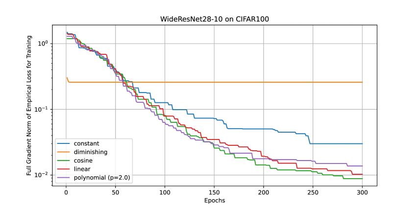
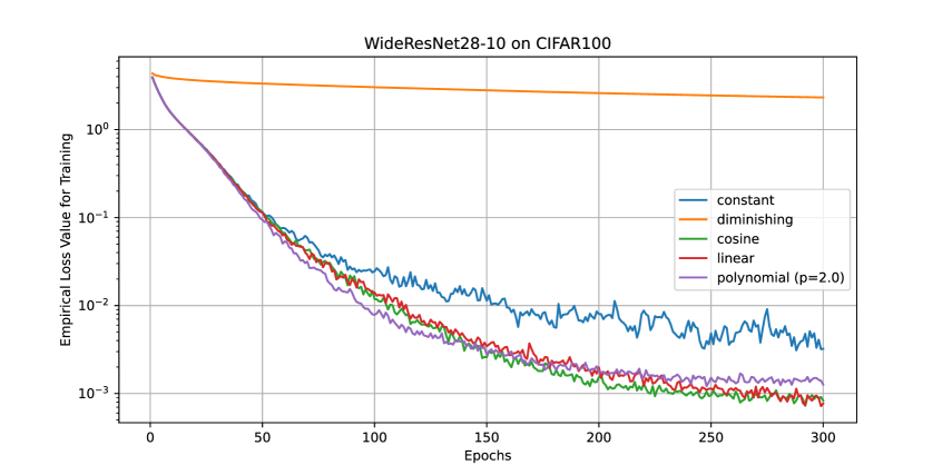
(a) Learning rate $\eta_{t}$ and batch size $b$ versus epochs	(b) Full gradient norm $\|\nabla f(\bm{\theta}_{e})\|$ versus epochs
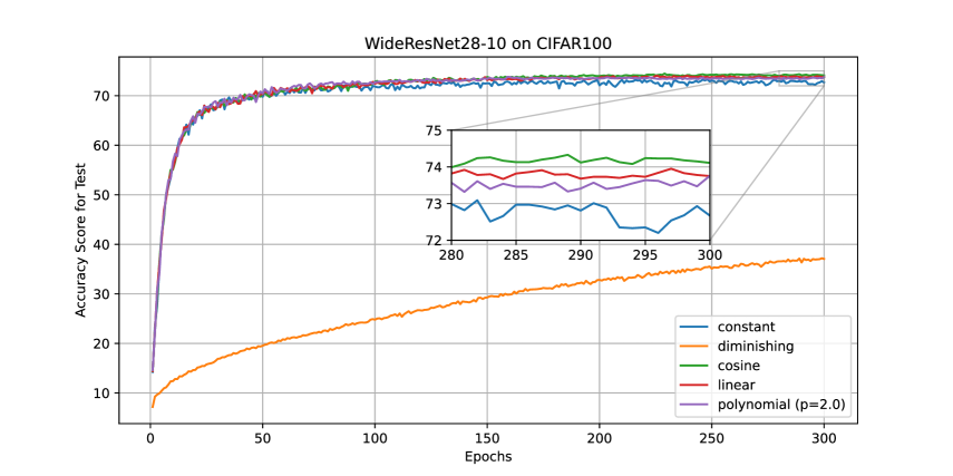
(c) Empirical loss $f(\bm{\theta}_{e})$ versus epochs	(d) Test accuracy score versus epochs

Figure 6: (a) Decaying learning rates (constant, diminishing, cosine, linear, and polynomial) and constant batch size, (b) full gradient norm of empirical loss, (c) empirical loss value, and (d) accuracy score in testing for SGD to train Wide-ResNet-28-10 on CIFAR100 dataset.

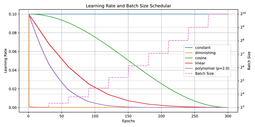
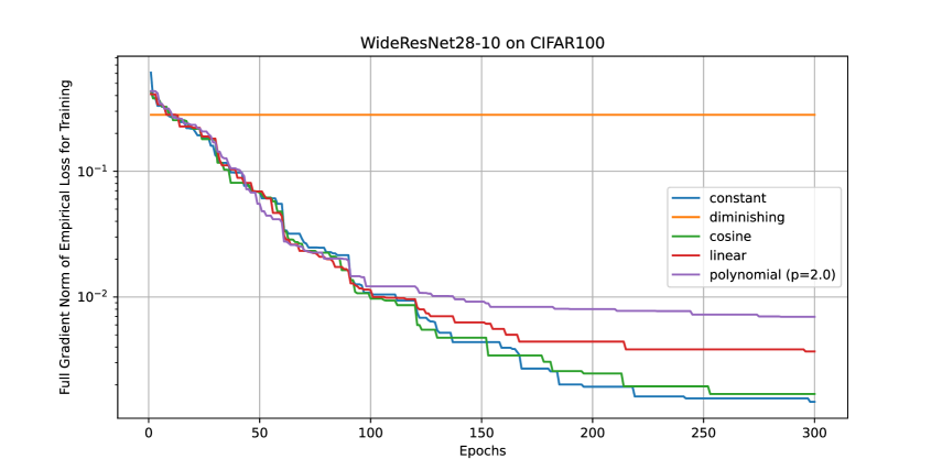
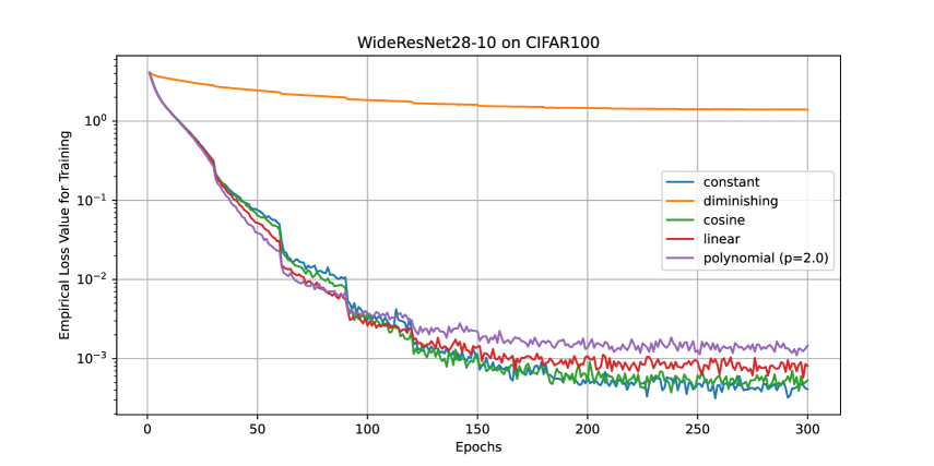
(a) Learning rate $\eta_{t}$ and batch size $b_{t}$ versus epochs	(b) Full gradient norm $\|\nabla f(\bm{\theta}_{e})\|$ versus epochs
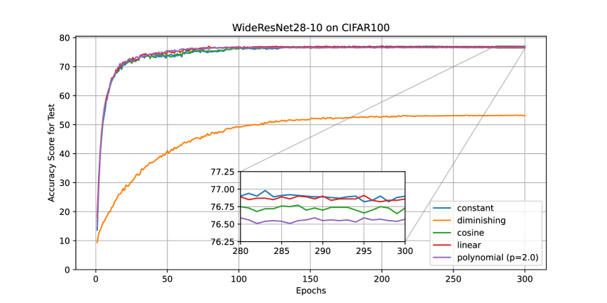
(c) Empirical loss $f(\bm{\theta}_{e})$ versus epochs	(d) Test accuracy score versus epochs

Figure 7: (a) Decaying learning rates and increasing batch size every 30 epochs, (b) full gradient norm of empirical loss, (c) empirical loss value, and (d) accuracy score in testing for SGD to train Wide-ResNet-28-10 on CIFAR100 dataset.

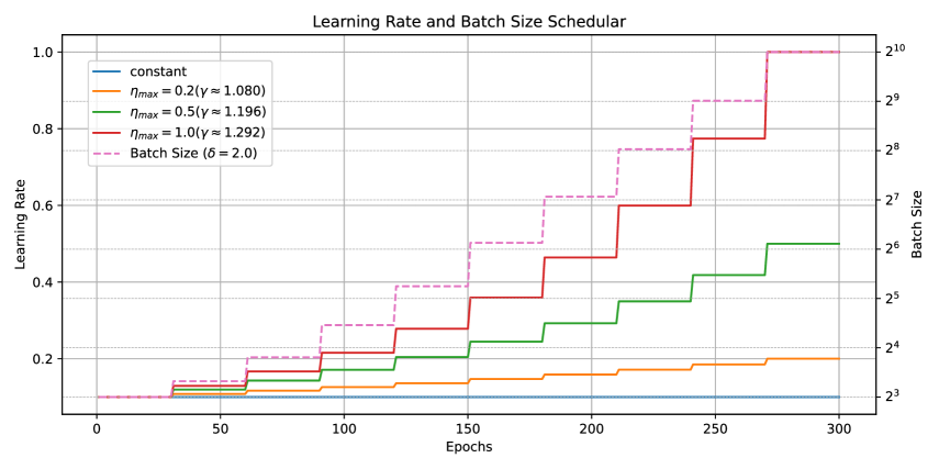
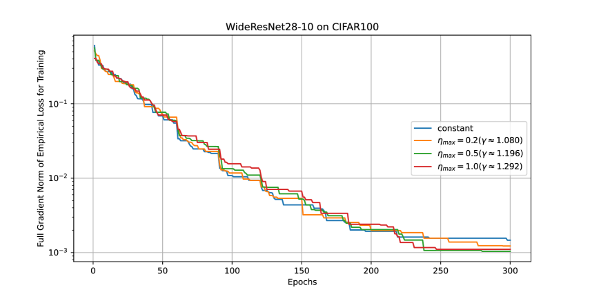
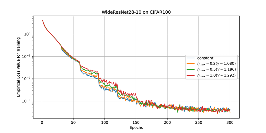
(a) Learning rate $\eta_{t}$ and batch size $b_{t}$ versus epochs	(b) Full gradient norm $\|\nabla f(\bm{\theta}_{e})\|$ versus epochs
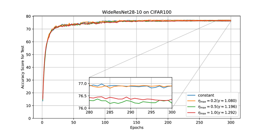
(c) Empirical loss $f(\bm{\theta}_{e})$ versus epochs	(d) Test accuracy score versus epochs

Figure 8: (a) Increasing learning rates ($\eta_{\max}=0.2,0.5,1.0$) and increasing batch size every 30 epochs, (b) full gradient norm of empirical loss, (c) empirical loss value, and (d) accuracy score in testing for SGD to train Wide-ResNet-28-10 on CIFAR100 dataset.

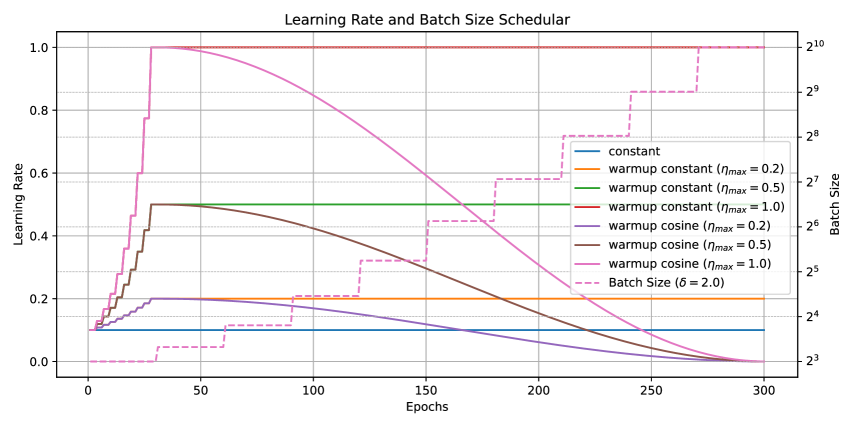
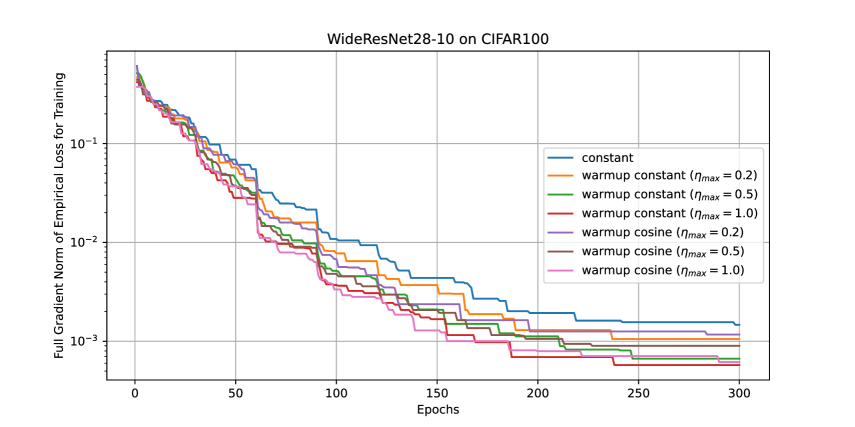
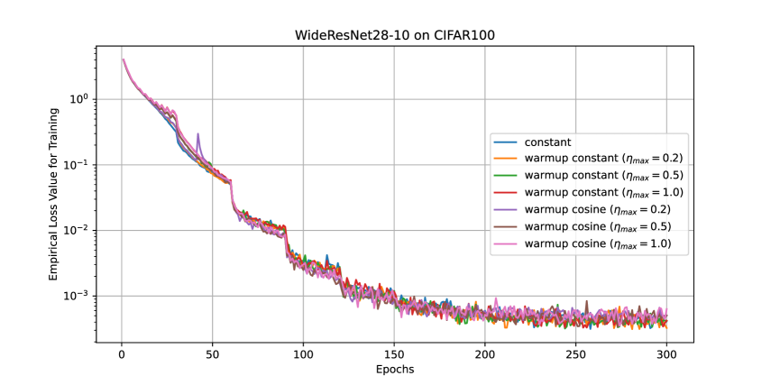
(a) Learning rate $\eta_{t}$ and batch size $b_{t}$ versus epochs	(b) Full gradient norm $\|\nabla f(\bm{\theta}_{e})\|$ versus epochs
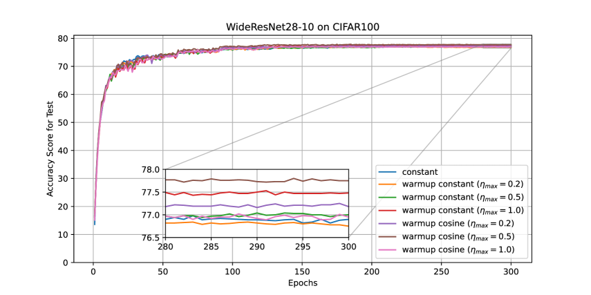
(c) Empirical loss $f(\bm{\theta}_{e})$ versus epochs	(d) Test accuracy score versus epochs

Figure 9: (a) Warm-up learning rates and increasing batch size every 30 epochs, (b) full gradient norm of empirical loss, (c) empirical loss value, and (d) accuracy score in testing for SGD to train Wide-ResNet-28-10 on CIFAR100 dataset.

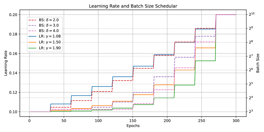
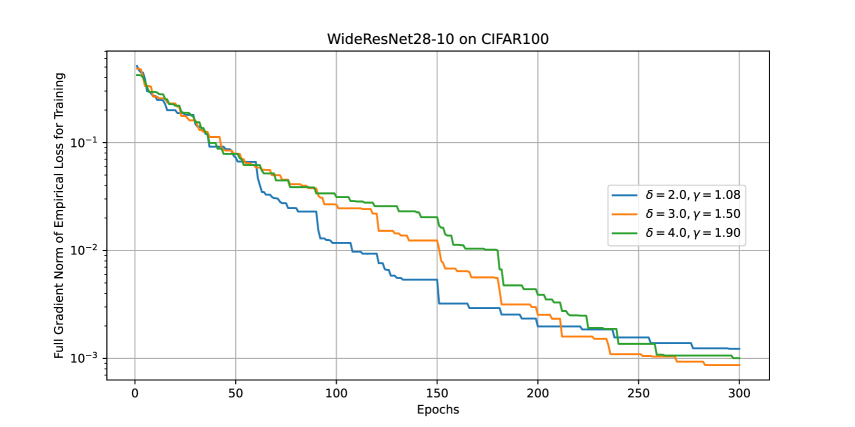
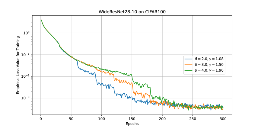
(a) Learning rate $\eta_{t}$ and batch size $b_{t}$ versus epochs	(b) Full gradient norm $\|\nabla f(\bm{\theta}_{e})\|$ versus epochs
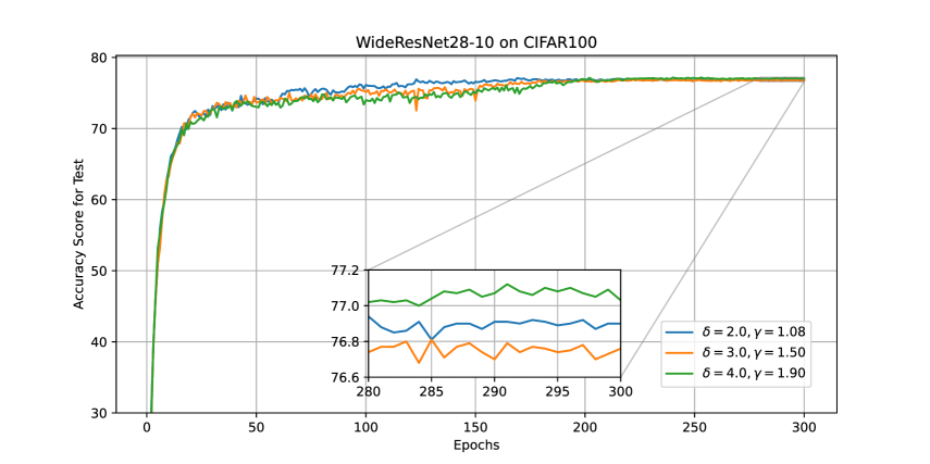
(c) Empirical loss $f(\bm{\theta}_{e})$ versus epochs	(d) Test accuracy score versus epochs

Figure 10: (a) Increasing learning rates and increasing batch sizes based on $\delta=2,3,4$, (b) full gradient norm of empirical loss, (c) empirical loss value, and (d) accuracy score in testing for SGD to train Wide-ResNet-28-10 on CIFAR100 dataset.

A.4 Training ResNet18 on Tiny ImageNet

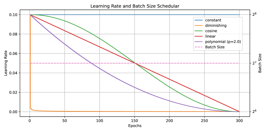
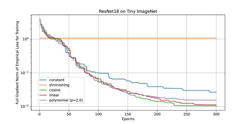
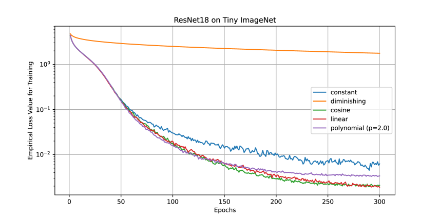
(a) Learning rate $\eta_{t}$ and batch size $b$ versus epochs	(b) Full gradient norm $\|\nabla f(\bm{\theta}_{e})\|$ versus epochs
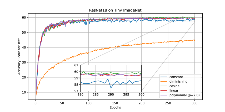
(c) Empirical loss $f(\bm{\theta}_{e})$ versus epochs	(d) Test accuracy score versus epochs

Figure 11: (a) Decaying learning rates (constant, diminishing, cosine, linear, and polynomial) and constant batch size, (b) full gradient norm of empirical loss, (c) empirical loss value, and (d) accuracy score in testing for SGD to train ResNet18 on Tiny ImageNet dataset.

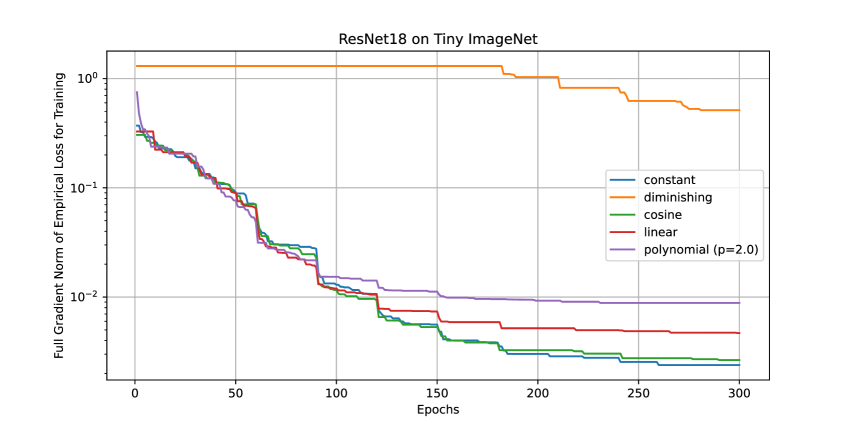
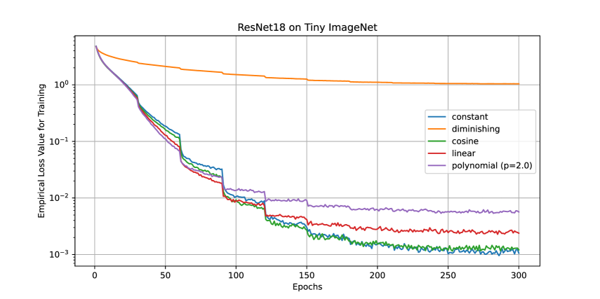
(a) Learning rate $\eta_{t}$ and batch size $b_{t}$ versus epochs	(b) Full gradient norm $\|\nabla f(\bm{\theta}_{e})\|$ versus epochs
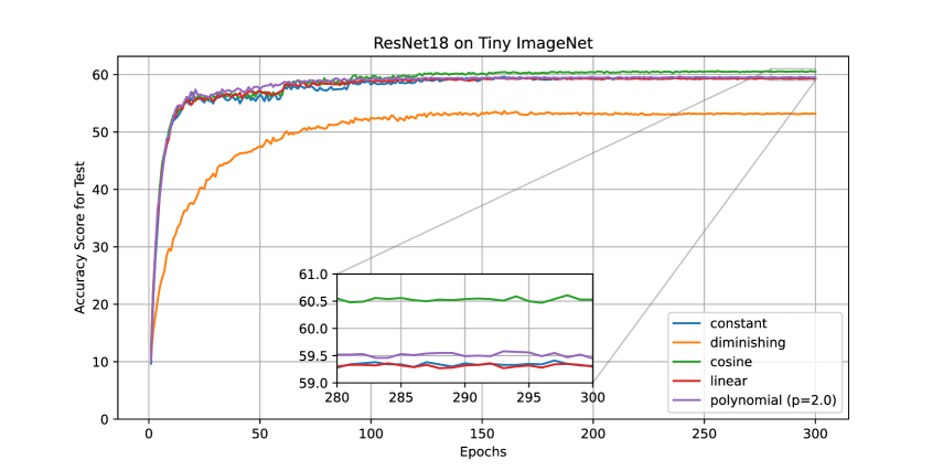
(c) Empirical loss $f(\bm{\theta}_{e})$ versus epochs	(d) Test accuracy score versus epochs

Figure 12: (a) Decaying learning rates and increasing batch size every 30 epochs, (b) full gradient norm of empirical loss, (c) empirical loss value, and (d) accuracy score in testing for SGD to train ResNet18 on Tiny ImageNet dataset.

(a) Learning rate $\eta_{t}$ and batch size $b_{t}$ versus epochs

(b) Full gradient norm $\|\nabla f(\bm{\theta}_{e})\|$ versus epochs

References

- Balles et al. (2016) Lukas Balles, Javier Romero, and Philipp Hennig. Coupling adaptive batch sizes with learning rates, 2016. Thirty-Third Conference on Uncertainty in Artificial Intelligence, 2017.
- Beck (2017) Amir Beck. First-Order Methods in Optimization. Society for Industrial and Applied Mathematics, Philadelphia, PA, 2017.
- Byrd et al. (2012) Richard H. Byrd, Gillian M. Chin, Jorge Nocedal, and Yuchen Wu. Sample size selection in optimization methods for machine learning. Mathematical Programming, 134(1):127–155, 2012.
- Chen et al. (2020) Hao Chen, Lili Zheng, Raed AL Kontar, and Garvesh Raskutti. Stochastic gradient descent in correlated settings: A study on Gaussian processes. In Advances in Neural Information Processing Systems, volume 33, 2020.
- Chen et al. (2018) Liang-Chieh Chen, George Papandreou, Iasonas Kokkinos, Kevin Murphy, and Alan L. Yuille. Deeplab: Semantic image segmentation with deep convolutional nets, atrous convolution, and fully connected crfs. IEEE Transactions on Pattern Analysis and Machine Intelligence, 40(4):834–848, 2018.
- De et al. (2017) Soham De, Abhay Yadav, David Jacobs, and Tom Goldstein. Automated Inference with Adaptive Batches. In Aarti Singh and Jerry Zhu (eds.), Proceedings of the 20th International Conference on Artificial Intelligence and Statistics, volume 54 of Proceedings of Machine Learning Research, pp. 1504–1513. PMLR, 2017.
- Fehrman et al. (2020) Benjamin Fehrman, Benjamin Gess, and Arnulf Jentzen. Convergence rates for the stochastic gradient descent method for non-convex objective functions. Journal of Machine Learning Research, 21:1–48, 2020.
- Ghadimi & Lan (2012) Saeed Ghadimi and Guanghui Lan. Optimal stochastic approximation algorithms for strongly convex stochastic composite optimization I: A generic algorithmic framework. SIAM Journal on Optimization, 22:1469–1492, 2012.
- Ghadimi & Lan (2013) Saeed Ghadimi and Guanghui Lan. Optimal stochastic approximation algorithms for strongly convex stochastic composite optimization II: Shrinking procedures and optimal algorithms. SIAM Journal on Optimization, 23:2061–2089, 2013.
- Gotmare et al. (2019) Akhilesh Gotmare, Nitish Shirish Keskar, Caiming Xiong, and Richard Socher. A closer look at deep learning heuristics: Learning rate restarts, warmup and distillation. In International Conference on Learning Representations, 2019.
- Goyal et al. (2018) Priya Goyal, Piotr Dollár, Ross Girshick, Pieter Noordhuis, Lukasz Wesolowski, Aapo Kyrola, Andrew Tulloch, Yangqing Jia, and Kaiming He. Accurate, large minibatch SGD: Training imagenet in 1 hour, 2018.
- He et al. (2016) Kaiming He, Xiangyu Zhang, Shaoqing Ren, and Jian Sun. Deep residual learning for image recognition. In Computer Vision and Pattern Recognition, pp. 770–778, 2016.
- He et al. (2019) T. He, Z. Zhang, H. Zhang, Z. Zhang, J. Xie, and M. Li. Bag of tricks for image classification with convolutional neural networks. In 2019 IEEE/CVF Conference on Computer Vision and Pattern Recognition, pp. 558–567, 2019.
- Hundt et al. (2019) Andrew Hundt, Varun Jain, and Gregory D. Hager. sharpDARTS: Faster and more accurate differentiable architecture search, 2019.
- Ioffe & Szegedy (2015) Sergey Ioffe and Christian Szegedy. Batch normalization: Accelerating deep network training by reducing internal covariate shift. In Francis Bach and David Blei (eds.), Proceedings of the 32nd International Conference on Machine Learning, volume 37 of Proceedings of Machine Learning Research, pp. 448–456, 2015.
- Khaled & Richtárik (2023) Ahmed Khaled and Peter Richtárik. Better theory for SGD in the nonconvex world. Transactions on Machine Learning Research, 2023.
- Liu et al. (2020) Liyuan Liu, Haoming Jiang, Pengcheng He, Weizhu Chen, Xiaodong Liu, Jianfeng Gao, and Jiawei Han. On the variance of the adaptive learning rate and beyond. In International Conference on Learning Representations, 2020.
- Loizou et al. (2021) Nicolas Loizou, Sharan Vaswani, Issam Laradji, and Simon Lacoste-Julien. Stochastic polyak step-size for SGD: An adaptive learning rate for fast convergence. In Proceedings of the 24th International Conference on Artificial Intelligence and Statistics, volume 130, 2021.
- Loshchilov & Hutter (2017) Ilya Loshchilov and Frank Hutter. SGDR: Stochastic gradient descent with warm restarts. In International Conference on Learning Representations, 2017.
- Lu (2024) Jun Lu. Gradient descent, stochastic optimization, and other tales, 2024.
- Nemirovski et al. (2009) Arkadi Nemirovski, Anatoli Juditsky, Guanghui Lan, and Alexander Shapiro. Robust stochastic approximation approach to stochastic programming. SIAM Journal on Optimization, 19:1574–1609, 2009.
- Robbins & Monro (1951) Herbert Robbins and Herbert Monro. A stochastic approximation method. The Annals of Mathematical Statistics, 22:400–407, 1951.
- Scaman & Malherbe (2020) Kevin Scaman and Cédric Malherbe. Robustness analysis of non-convex stochastic gradient descent using biased expectations. In Advances in Neural Information Processing Systems, volume 33, 2020.
- Shallue et al. (2019) Christopher J. Shallue, Jaehoon Lee, Joseph Antognini, Jascha Sohl-Dickstein, Roy Frostig, and George E. Dahl. Measuring the effects of data parallelism on neural network training. Journal of Machine Learning Research, 20:1–49, 2019.
- Smith et al. (2018) Samuel L. Smith, Pieter-Jan Kindermans, and Quoc V. Le. Don’t decay the learning rate, increase the batch size. In International Conference on Learning Representations, 2018.
- Vaswani et al. (2017) Ashish Vaswani, Noam Shazeer, Niki Parmar, Jakob Uszkoreit, Llion Jones, Aidan N. Gomez, Lukasz Kaiser, and Illia Polosukhin. Attention is All you Need. In Advances in Neural Information Processing Systems, volume 30, 2017.
- Vaswani et al. (2019) Sharan Vaswani, Aaron Mishkin, Issam Laradji, Mark Schmidt, Gauthier Gidel, and Simon Lacoste-Julien. Painless stochastic gradient: Interpolation, line-search, and convergence rates. In Advances in Neural Information Processing Systems, volume 32, 2019.
- Wang et al. (2021) Xiaoyu Wang, Sindri Magnússon, and Mikael Johansson. On the convergence of step decay step-size for stochastic optimization. In Advances in Neural Information Processing Systems, 2021.
- Wu et al. (2014) Yuting Wu, Daniel J. Holland, Mick D. Mantle, Andrew G. Wilson, Sebastian Nowozin, Andrew Blake, and Lynn F. Gladden. A Bayesian method to quantifying chemical composition using NMR: Application to porous media systems. In 2014 22nd European Signal Processing Conference, pp. 2515–2519, 2014.
- Zhang et al. (2019) Guodong Zhang, Lala Li, Zachary Nado, James Martens, Sushant Sachdeva, George E. Dahl, Christopher J. Shallue, and Roger Grosse. Which algorithmic choices matter at which batch sizes? Insights from a noisy quadratic model. In Advances in Neural Information Processing Systems, volume 32, 2019.
- Zinkevich (2003) Martin Zinkevich. Online convex programming and generalized infinitesimal gradient ascent. In Proceedings of the 20th International Conference on Machine Learning, pp. 928–936, 2003.