Measure-Theoretic Time-Delay Embedding

Abstract

The celebrated Takens’ embedding theorem provides a theoretical foundation for reconstructing the full state of a dynamical system from partial observations. However, the classical theorem assumes that the underlying system is deterministic and that observations are noise-free, limiting its applicability in real-world scenarios. Motivated by these limitations, we rigorously establish a measure-theoretic generalization that adopts an Eulerian description of the dynamics and recasts the embedding as a pushforward map between probability spaces. Our mathematical results leverage recent advances in optimal transportation theory. Building on our novel measure-theoretic time-delay embedding theory, we have developed a new computational framework that forecasts the full state of a dynamical system from time-lagged partial observations, engineered with better robustness to handle sparse and noisy data. We showcase the efficacy and versatility of our approach through several numerical examples, ranging from the classic Lorenz-63 system to large-scale, real-world applications such as NOAA sea surface temperature forecasting and ERA5 wind field reconstruction.

1 Introduction

Dynamical systems provide a universal language for modeling the temporal evolution of complex systems, appearing across a diverse range of scientific disciplines, including physics, biology, chemistry, ecology, and social sciences. A dynamical system comprises of a space (denoted by $M$) defining the possible states ($x$) of the system and a rule describing the evolution of these states over time ($t$). Understanding the behavior of complex dynamics allows for accurate predictions of future states based on historical data, which is crucial in fields such as weather prediction, financial market analysis, and epidemiology [45, 21, 33, 57, 8, 2, 26].

In practice, the exact equations governing a system’s behavior are often unknown, and one may have to study the system’s evolution through empirically collected time series data. This indirect interaction with the system’s full dynamics is frequently complicated by experimental limitations preventing complete measurement of the full state. For instance, only the first coordinate of a $d$-dimensional state $x$ may be observed. Such partial and potentially limited observational data makes it challenging to accurately model the system’s dynamics.

In situations where the full state is not directly observable, time-delay embedding has become a fundamental technique in the analysis of dynamical systems. This method involves concatenating time-lagged versions of a scalar time-dependent observation into a high-dimensional state vector, resulting in a system that is topologically equivalent to the full, unobserved dynamics. The celebrated Takens’ embedding theorem supplies the theoretical foundation for time-delay embedding and has inspired a myriad of works over the last four decades that perform data-driven analysis on partially observed nonlinear systems [50, 27]. Notable applications of time-delay embedding include forecasting [4, 58], noise reduction [22, 29], control [37], as well as various biological studies [57, 40, 46].

However, Takens’ embedding theorem assumes that the underlying system follows precise, predictable rules without random perturbations and that observables are measured perfectly without errors. In practical scenarios, both the underlying system and the observables are subject to intrinsic and extrinsic noise. Intrinsic noise refers to the inherent unpredictability within the system, such as thermal fluctuations or quantum effects, while extrinsic noise includes measurement errors, environmental disturbances, and observational limitations–external factors that can affect the data. These sources of randomness challenge the idealized assumptions of Takens’ theorem when modeling partially observed dynamical systems.

Given these practical challenges, it is necessary to consider variants of time-delay embedding that incorporate assumptions of randomness. Notably, it was shown in [44] that the time-delay map is an embedding almost surely in the space of observation functions, and in [5] that the delay map formed by a polynomially perturbed observation function is an embedding at almost all points. However, these works do not address intrinsic or extrinsic noise in the state itself. On the other hand, [14] leverages statistical techniques to quantify the effect of i.i.d. extrinsic noise on state reconstruction and time-series prediction. Approaches incorporating stochasticity often face the curse of dimensionality. For example, [47, 48] showed that Takens’ theorem holds for stochastically forced systems whose vector fields lie in finite discrete probability spaces. Nevertheless, the embedding dimension increases with the dimension of the probability space, and for general stochastic systems with an infinite-dimensional sample space, such variants of time-delay embedding no longer hold.

In this work, we take a different approach by lifting both the domain ($M$) and the co-domain ($N$) of an embedding map $\Phi:M\to N$ to the space of probability measures over $M$ and $N$, respectively, denoted by $\mathcal{P}(M)$ and $\mathcal{P}(N)$. These two infinite-dimensional probability spaces are connected by pushforward maps acting on probability measures (see Fig. 1). One main contribution of our work is to rigorously study the embedding property between $\mathcal{P}(M)$ and $\mathcal{P}(N)$ under an Eulerian description of the dynamics. We establish the existence of a smooth, one-to-one, and structure-preserving map that translates fluid/gas flows represented as probability distributions over the state coordinates into their counterparts characterized in the time-delay coordinates. Moreover, this probabilistic embedding map is precisely the pushforward action of the original Lagrangian embedding map $\Phi$. The theory of optimal transport [54] plays a critical role in the analysis, supplying essential mathematical tools such as the differentiability of maps between probability spaces and tangent space structures.

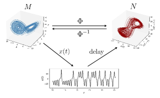
(a)

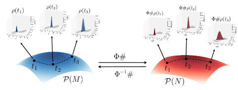
(b)

Figure 1: Illustration of the differences between the classical pointwise time-delay embedding (a) and the proposed measure-theoretic time-delay embedding (b).

Our second main contribution is leveraging the measure-theoretic time-delay embedding theory to establish a robust computational framework for learning the inverse embedding function ($\Phi^{-1}$) from data. This function, known as the full-state reconstruction map, typically has no analytical form but is crucial for forecasting the complete state of a nonlinear system from partially observed data. To learn the reconstruction map, we first extract empirical measures in both the full-state space ($M$) and the delay space ($N$) based on a single time trajectory. We then select a suitable metric over the probability space as the objective function and enforce that the pushforwards of the empirical measures in the delay space match the corresponding measures in the full-state space. In contrast with our approach, existing methods commonly learn the reconstruction map using the pointwise mean-squared error loss [4, 40, 58]. When the observed data is sparse and noisy, the accuracy of such pointwise methods can be compromised, while our measure-theoretic approach demonstrates clear robustness. In Section 4, we showcase the effectiveness of our proposed approach through various numerical tests on classic synthetic examples, such as the Lorenz-63 and Lotka–Volterra systems, as well as large-scale real-world applications, including the reconstruction of NOAA Sea Surface Temperature [41] and ERA5 wind speed datasets from partial observations [24].

The rest of the paper is organized as follows. Section 2 reviews the essential background on Takens’ theorem and optimal transport. In Section 3, we present our main theoretical result, which generalizes Takens’ theorem to the space of probability distributions. In Section 4, we introduce our computational framework for learning the inverse embedding map from data and demonstrate its robustness across several synthetic and real data examples. Conclusions follow in Section 5.

2 Background and Overview

Essential mathematical notations are summarized in Table 1.

2.1 Takens’ Embedding Theorem

Many physical processes can be modeled by systems of ordinary differential equations (ODEs), which can be represented in the form $\dot{x}=v(x)$, where $x\in M$ is the state, $M$ is a smooth compact $d$-dimensional manifold and $v$ is a $\mathcal{C}^{2}$ vector field on $M$. Given an initial condition $x\in M$, we denote the solution to the ODE by $\{\phi_{t}(x)\}_{t\geq 0}$, which is often referred to as the trajectory. Moreover, $\phi_{t}:M\to M$ is known as the time-$t$ flow map. The trajectory provides critical information about the underlying dynamical system and is useful in various engineering and data science applications, such as parameter identification and model reduction [7, 11]. However, when the state dimension $d$ is large, it is often the case that experimentalists are unable to directly access the trajectory $\{\phi_{t}(x)\}_{t\geq 0}$, but instead have access to time-series projections of the form $\{h(\phi_{t}(x))\}_{t\geq 0},$ where $h\in\mathcal{C}^{2}(M,\mathbb{R})$ is an observation function. Thus, it is essential to understand to what extent the time series $\{h(\phi_{t}(x))\}_{t\geq 0}$ can provide information on the full trajectory $\{\phi_{t}(x)\}_{t\geq 0}$.

Takens’ embedding theorem (1981) establishes criteria under which the partial observations of a dynamical system can be used to reconstruct the full state. This reconstruction is possible because the original trajectory $\{\phi_{t}(x)\}_{t\geq 0}$ and the time-lags of the partially observed trajectory $\{h(\phi_{t}(x))\}_{t\geq 0}$ are related through a structure-preserving diffeomorphism, known as an embedding. A precise definition is given in Definition 1 below.

Definition 1 (Embedding).

Let $M,N$ be two differentiable manifolds. Then a function $f:M\to N$ is an embedding if $f$ is a diffeomorphism such that the derivative operator $Df_{x}:T_{x}M\to T_{f(x)}N$ is injective $\forall x\in M$.

The statement of Takens’ theorem is given in Theorem 1.

Theorem 1 (Takens’ Embedding Theorem).

Let $\tau>0$, choose $m\geq 2d+1$, and suppose that $v$ satisfies the following:

1. If $v(x)=0$, then the eigenvalues of $(d\phi_{\tau})_{x}:T_{x}M\rightarrow T_{\phi_{\tau}(x)}M$ are all different, and none of them equals $1$.

2. No periodic integral curve of $v$ has period equal to $k\tau$ for $k\in\{1,\dots,m\}$.

Then, it is a generic property that the delay coordinate map given by

$$\Phi_{h,\phi_{\tau}}(x):=\left(h(x),h(\phi_{\tau}(x)),\dots,h\left(\phi_{(m-1)\tau}(x)\right)\right)\in\mathbb{R}^{m}\,,$$ (1)

is an embedding.

Notation	Meaning
$M$	Compact $d$ dimensional manifold
$\phi_{t}$	The flow map of a dynamical system on $M$
$h$	The observation function $h:M\rightarrow\mathbb{R}$
$\tau$	The delay parameter belonging to $\mathbb{R}_{>0}$
$m$	Dimension of the delay embedding space
$\rho$, $\rho_{0}$	Measures on $M$
$\Phi_{h,\phi_{\tau}}$	Takens’ delay embedding map
$\Psi_{h,\phi_{\tau}}$	The delay embedding map for distributions
$\rho_{t}$	Curve of measures starting at $\rho_{0}=\rho$
$|\rho_{t}^{\prime}|$	Metric derivative of $\rho_{t}$ according to Definition 4
$\frac{d}{dt}\rho_{t}=v_{t}$	Tangent vector field along the curve $\rho_{t}$ as in Definition 6
$\mathcal{F}(X,Y)$	The space of measurable functions from $X$ taking values in $Y$

Table 1: A list of mathematical notations in Section 2 and Section 3.

In (1), $m\in\mathbb{N}$ is known as the embedding dimension, and $\tau>0$ is the so-called time-delay. By “generic” we mean that the collection of observation functions $h\in C^{2}(M,\mathbb{R})$ for which (1) defines an embedding is open and dense in the $C^{2}$ topology. In particular, when (1) is an embedding, the delayed trajectory $\{\Phi_{h,\phi_{\tau}}(\phi_{t}(x))\}_{t\geq 0}$ is topologically equivalent to the original orbit $\{\phi_{t}(x)\}_{t\geq 0}\subseteq M$. This perspective has motivated the use of delay coordinates in various applications, such as time-series prediction [17], attractor reconstruction [38], causality detection [49], and noise reduction [22, 29].

Often, dynamical systems asymptotically approach a compact attractor $A$ with fractal dimension $d_{A}\ll d$. Ideally, the embedding dimension should depend on $d_{A}$ rather than $d$, in order to ensure that the attractor $A$ is embedded using the delay map. In [44], Takens’ theorem is generalized along these lines when the flow map $\phi_{t}$ is defined on an open subset $U$ of Euclidean space.

In a practical setting, only the time-series projection $\{h(\phi_{t}(x))\}_{t\geq 0}$ is available, and neither $d$ nor $d_{A}$ is known a priori. Additionally, the time series may be corrupted by noise. Therefore, optimally selecting the embedding dimension $m\in\mathbb{N}$ and the time delay $\tau>0$ from this limited information is crucial for ensuring the usefulness of the delay map in applications. Various data-driven techniques have been explored to determine these parameters numerically from the time series $\{h(\phi_{t}(x))\}_{t\geq 0}$, including False Nearest Neighbors [42], Cao’s method [13], mutual information [20, 34], and approaches based on persistent homology [51]. In this work, we will assume that the time delay $\tau$ and the embedding dimension $m$ have already been chosen using these techniques.

2.2 Optimal Transport and the Wasserstein Geometry

A central goal of this work is to lift the statement of Takens’ embedding theorem (Theorem 1) to the space of probability measures over the underlying manifold $M$. Using tools from optimal transport theory, we will rigorously define the equivalent notions, in a measure-theoretic setting, to those presented in Theorem 1.

The space of probability measures on $M$ is given by $\mathcal{P}(M)=\{\mu\in\mathcal{B}(M):\mu(M)=1\}$, where by $\mathcal{B}(M)$ we denote the space of all Borel measures over $M$. Any map $h:M\rightarrow N$ can be lifted to a map from $\mathcal{P}(M)$ to $\mathcal{P}(N)$ by the pushforward operator defined below.

Definition 2 (The pushforward operator [1]).

The pushforward operator lifts maps from $M$ to $N$ to maps between the equivalent spaces of probability measures and is defined by

$$h\#\mu(B)=\mu(h^{-1}(B)),\ \forall h\in\mathcal{F}(M,N),\,\,\forall B\in\mathcal{B}(N)\,.$$ (2)

Equivalently, $\int_{M}r(h(x))\,{\mathrm{d}}\mu(x)=\int_{N}r(x)\,{\mathrm{d}}(h\#\mu)(x)$, for every bounded, Borel measurable function $r:N\rightarrow\mathbb{R}$.

2.2.1 The continuity equation

For the rest of this paper, we will restrict our study to the space of probability measures that have finite second-order moments, $\mathcal{P}_{2}(M)=\{\mu\in\mathcal{P}(M)\ :\ \int|x|^{2}\,{\mathrm{d}}\mu<\infty\}$. In this space, we can use the differential structure of the quadratic Wasserstein metric. Let us consider a curve through $\mathcal{P}_{2}(M)$, which will be the Eulerian equivalent to the Lagrangian flow $\phi_{t}$ on $M$ in Theorem 1.

A first requirement for $\phi_{t}$ to be a flow is continuity. In the context of flows on $\mathcal{P}_{2}(M)$, the equivalent notion is absolute continuity. To achieve this, we require $M$ to be a metric space and assume $\mathfrak{D}:\mathcal{P}_{2}(M)\times\mathcal{P}_{2}(M)\rightarrow\mathbb{R}_{\geq 0}$ is a distance between probability measures. In particular, if $M$ is a smooth compact manifold, there always exists a metric for $M$ and we can view $M$ as a metric space.

Definition 3 (Absolute continuity of curves and maps [1]).

1. We say a curve $\rho_{t}:[0,1]\rightarrow\mathcal{P}_{2}(M)$ is absolutely continuous if $\mathfrak{D}(\rho_{t},\rho_{s})\leq\int_{t}^{s}f(x)\,{\mathrm{d}}x$, where $f$ is an $L^{1}$ function from $[0,1]$ to $\mathbb{R}$.

2. A map $F:\mathcal{P}_{2}(M)\rightarrow\mathcal{P}_{2}(N)$ is absolutely continuous if for every absolutely continuous curve $\rho_{t}\in\mathcal{P}_{2}(M)$, $F(\rho_{t})$ is absolutely continuous in $\mathcal{P}_{2}(N)$, up to redefining $t\mapsto\rho_{t}$ on a set of zero Lebesgue measure on $[0,1]$.

We will use the shorthand notation “AC” for “absolute continuous” hereafter. A useful property of AC curves is that they are metric differentiable. Later, we will employ the metric derivative to bound the norm of tangent vectors (see Proposition 3).

Definition 4 (Metric derivative [1]).

For any AC curve $\rho_{t}\in\mathcal{P}_{2}(M)$, the limit

$$|\rho_{t}^{\prime}|=\lim_{s\to t}\frac{\mathfrak{D}(\rho_{t},\rho_{s})}{|t-s|}$$ (3)

exists $L^{1}$ a.e. in $t$, and is called the metric derivative of $\rho_{t}$.

In Theorem 1, the flow $\phi_{t}$ is generated by a smooth vector field $v:M\rightarrow TM$, such that at every point $\frac{d}{dt}\phi_{t}(x)=v(x)$. In contrast, in the Wasserstein space, the curve $\rho_{t}$ is generated by a square-integrable vector field

$$v_{t} \in L^{2}(TM,\rho_{t})=\Big{\{}v:[0,T]\times M\rightarrow TM,\,$$

$$\|v_{t}\|_{L^{2}(\rho_{t})}:=\sqrt{\int_{M}g_{x}(v_{t}(x),v_{t}(x)){\mathrm{d}}\rho_{t}(x)}<\infty\Big{\}},$$

where $g_{x}$ is the Riemannian metric on $M$. Note that $v_{t}(x)\in T_{x}M$ and $g_{x}:T_{x}M\times T_{x}M\rightarrow\mathbb{R}$. This vector field $v_{t}$ has to additionally satisfy the continuity equation ((4)) in the distributional sense (see (5)):

$$\frac{\partial\rho_{t}}{\partial t}+\nabla\cdot(v_{t}\rho_{t})=0\,.$$ (4)

To be more precise,

$$\int_{0}^{T}\int_{M}\left(\frac{\partial\varphi(x,t)}{\partial t}+v_{t}(x)\cdot\nabla\varphi(x,t)\right){\mathrm{d}}\rho_{t}(x){\mathrm{d}}t=0,$$ (5)

for all $\varphi\in\mathcal{D}(M\times[0,T])\,$ where $\mathcal{D}(M\times[0,T])$ denotes the space of test functions on $M\times[0,T]$ (see Remark 2). This continuity equation comes from the conservation of mass. In the rest of the paper, when we say that the continuity equation is satisfied, we mean (5) holds. Theorem 2 below shows that any AC curve is a solution to (5) for an appropriate choice of $v_{t}$ [1, Chapter 8].

Theorem 2.

Let $v_{t}$ be a Borel vector field such that:

1. $\int_{0}^{T}\int_{M}|v_{t}(x)|d\mu_{t}(x)\,{\mathrm{d}}t<\infty$ ,

2. $\int_{0}^{T}\sup\limits_{B}\left(|v_{t}|+\text{Lip}(v_{t},B)\right)\,{\mathrm{d}}t<\infty$ ,

where $\text{Lip}(v_{t},B)$ denotes the Lipscitz constant of $v_{t}$ on the set $B\in M$. Let $\phi_{t}:M\times[0,T]\rightarrow M$ be the solution to the ODE

$$\phi_{t}(x,s)=x,\qquad\frac{d}{dt}\phi_{t}(x,s)=v_{t}(\phi_{t}(x,s)).$$ (6)

Suppose that for $\rho_{0}$-a.e. $x\in M$, $t<\sup(I(x,0))$ for $t\in[0,T]$, where $I(x,0)$ denotes the interval on which solutions to (6) at $s=0$ and position $x$ exist. Then,

$$\rho_{t}=\phi_{t}\#\rho_{0}$$

solves the continuity equation. Conversely, let $v_{t}$ be a Borel vector field satisfying conditions (i) and (ii). Let $\rho\in\mathcal{P}_{2}(M)$ and define $\rho_{t}=\phi_{t}\#\rho$, where $\phi_{t}$ is the flow of the system $\dot{x}=v_{t}(x)$. Then $\rho_{t}$ is the unique solution to the continuity equation with initial condition $\rho$.

Remark 1.

This theorem establishes the connection between the deterministic dynamical system on $M$ and its lifted version on $\mathcal{P}_{2}(M)$. Thus, it enables us to lift the differential structure to $\mathcal{P}_{2}(M)$ and show that tangent vectors indeed exist. For more details see Section 2.2.2.

Remark 2.

Without loss of generality, we will work with test functions that are compactly supported and continuously differentiable on $M\times[0,T]$, i.e., $\mathcal{D}(M\times[0,T])=\mathcal{C}^{1}_{c}(M\times[0,T])$. This gives us sufficient regularity to define all the distributional derivatives of $\rho$ and $v_{t}$. Moreover, it can be shown (see [1, Remark 8.1.1]) that if (5) holds for any $\varphi\in\mathcal{D}(M\times[0,T])$, it also holds for $\varphi\in\mathcal{C}^{\infty}_{c}(M\times[0,T])$. Similarly, for time-independent test functions, we can choose $\mathcal{D}(M)=\mathcal{C}^{1}_{c}(M)$. The same extends to test functions for $N$ and $N\times[0,T]$.

2.2.2 The tangent space of $\mathcal{P}_{2}(M)$

Hereafter, we assume $(M,g)$ is a Riemannian manifold and $g$ is the Riemannian metric. The tangent space to a manifold at a specific point is comprised of all possible infinitesimal directions of motion starting from that point. The continuity equation ((4)) tells us how a measure evolves in time along the direction specified by a vector field $v_{t}$, and Theorem 2 verifies the existence of such directions. Hence, intuitively, we may define $T_{\rho}\mathcal{P}_{2}(M)=L^{2}(TM,\rho)$ as the tangent space to $\mathcal{P}_{2}(M)$ at $\rho$. However, not every element in $L^{2}(TM,\mu)$ generates a different flow in $\mathcal{P}_{2}(M)$.

Remark 3 (Non-uniqueness).

Fix an AC curve $\rho_{t}$ and consider $v_{t},w_{t}\in L^{2}(TM,\rho_{t})$ where $\nabla\cdot(w_{t}\rho_{t})=0$ and $v_{t}$ satisfies $\partial_{t}\rho_{t}+\nabla\cdot(v_{t}\rho_{t})=0$ (the existence of $v_{t}$ is guaranteed by Theorem 2). Then one can check that $\rho_{t}$ also satisfies $\partial_{t}\rho_{t}+\nabla\cdot((v_{t}+w_{t})\rho_{t})=0$. Hence, any two vector fields that differ by a $\rho_{t}$-weighted divergence-free component produce the same solution to the continuity equation. We say a vector field $v$ is $\rho$-weighted divergence-free if $\nabla\cdot(v\rho)=0$ holds in the distributional sense, i.e., $\forall\varphi\in\mathcal{D}(M):\int_{M}g_{x}\left(\nabla\varphi(x),v(x)\right)\,{\mathrm{d}}\rho(x)=0$. A time-dependent vector field $v_{t}$ is divergence free if the above holds for $L^{1}$-a.e. $t$.

To choose a unique element that specifies the infinitesimal direction in $\mathcal{P}_{2}(M)$, we need to project out the $\rho$-weighted divergence-free component. This leads to the following definition of the Wasserstein tangent space.

Definition 5 (Wasserstein tangent space).

The three definitions below are equivalent [55].

1. The tangent space $T_{\rho}\mathcal{P}_{2}(M)=L^{2}(TM,\rho)/\sim$, where $v\sim w\iff\forall\varphi\in\mathcal{D}(M)$,

   $$\int_{M}g_{x}\left(\nabla\varphi(x),v(x)-w(x)\right)\,{\mathrm{d}}\rho(x)=0.$$ (7)

2. $T_{\rho}\mathcal{P}_{2}(M)=\{v\in L^{2}(TM,\rho):\|v+w\|_{L^{2}(\rho)}\geq\|v\|_{L^{2}(\rho)}$, $\forall w\in L^{2}(TM,\rho)\text{ such that }\nabla\cdot(w\rho)=0\}$.

3. $T_{\rho}\mathcal{P}_{2}(M)$ is the closure of the space of all gradients of test functions on $M$ in $L^{2}_{\rho}$, i.e.,

   $$T_{\rho}\mathcal{P}_{2}(M)=\overline{\{\nabla\varphi,\ \varphi\in C_{c}^{\infty}(M)\}}^{L^{2}_{\rho}}.$$

Remark 4 (Equality in $T_{\rho}\mathcal{P}_{2}(M)$).

Based on Definition 5, $v,w\in T_{\rho}\mathcal{P}_{2}(M)$ are equal if (7) holds. Equivalently, $v\neq w$ in $T_{\rho}\mathcal{P}_{2}(M)$ if $\exists\varphi\in\mathcal{D}(M)$ such that

$$\int_{M}g_{x}(\nabla\varphi(x),v(x)-w(x)){\mathrm{d}}\rho(x)\neq 0\,.$$

2.2.3 The projection operator

For any $w\in L^{2}(TM,\rho)$, one can obtain an element of $T_{\rho}\mathcal{P}_{2}(M)$ by projection:

$$w=v+v^{\perp},\,\,\,P^{\rho}(w):=v\in T_{\rho}\mathcal{P}_{2}(M),\,\,\,v^{\perp}\in T^{\perp}_{\rho}\mathcal{P}_{2}(M),\,$$ (8)

where $T_{\rho}^{\perp}\mathcal{P}_{2}(M)$ is the orthogonal complement of $T_{\rho}\mathcal{P}_{2}(M)$ with respect to the $\rho$-weighted $L^{2}$ inner product, and $P^{\rho}:L^{2}(TM,\rho)\rightarrow T_{\rho}\mathcal{P}_{2}(M)$ is the projection operator. We will use this projection operator to obtain the unique vector field defining the derivative of a map between probability spaces. The kernel of $P^{\rho}$ comprises all $\rho$-weighted divergence-free vector fields $w$ such that $\nabla\cdot(\rho w)=0$ in the distributional sense. One important property of $P^{\rho}$ is given in Proposition 1, whose complete proof is in the supplementary materials.

Proposition 1.

Let $(M,g)$ be a Riemannian manifold. Then for all $v\in L^{2}(TM,\rho)$ and any $\varphi\in\mathcal{D}(M)$,

$$\int_{M}g_{x}(\nabla\varphi(x),P^{\rho}v(x)){\mathrm{d}}\rho(x)=\int_{M}g_{x}(\nabla\varphi(x),v){\mathrm{d}}\rho(x).$$

2.2.4 Metric change of variables formula

We review the following result from Riemannian geometry, which will be used to show the injectivity of the metric derivative operator (see the proof of Theorem 4). A complete proof appears in the supplementary materials.

Proposition 2.

Let $(M,g)$ and $(N,q)$ be Riemannian manifolds, $f:M\rightarrow N$ be a differentiable map and $\varphi\in\mathcal{D}(N)$. Then for all $X\in TM$,

$$g_{x}(\nabla(\varphi\circ f)(x),X(x))=q_{f(x)}\Big{(}(\nabla\varphi)(f(x)),df_{x}X(x)\Big{)}.$$ (9)

3 Measure-Theoretic Time-Delay Embedding

In this section, we establish our main theoretical result on the measure-theoretic time-delay embedding. In the classic Takens’ embedding (Theorem 1), there are three key components: (1) the flow $\phi_{t}$ generated by the vector field $v$, (2) the observable $h$, and (3) the notion of an embedding. To extend Takens’ embedding to probability measures, we will find the equivalent objects to each of these three components in the space of probability distributions.

3.1 Differentiable curves in $\mathcal{P}_{2}(M)$

On the Lagrangian level, given an initial condition $x_{0}$, the flow $\phi_{t}(x_{0})$ generates a differentiable curve $x(t)=\phi_{t}(x_{0})$ in $M$. Similarly, on the Eulerian level, we want to have a differentiable curve $\rho_{t}$ and a vector field $v_{t}\in T_{\rho_{t}}\mathcal{P}_{2}(M)$ such that they satisfy the continuity equation ((4)). To begin with, we define the notion of a vector field along a curve in $\mathcal{P}_{2}(M)$.

Definition 6 (Vector fields along the curves).

Consider a curve $\rho_{t}\in\mathcal{P}_{2}(M)$. We say that $v_{t}:[0,1]\rightarrow T_{\rho_{t}}\mathcal{P}_{2}(M)$ is a vector field along the curve $\rho_{t}$ if the tuple $(\rho_{t},v_{t})$ satisfies the continuity equation ((4)). If such a vector field exists, we denote it by $v_{t}:=\frac{d}{dt}\rho_{t}$.

This allows us to define differentiable curves in $\mathcal{P}_{2}(M)$.

Definition 7 (Differentiable curve).

A curve $\rho_{t}$ in $\mathcal{P}_{2}(M)$ is differentiable if there exists a vector field $v_{t}\in T_{\rho_{t}}\mathcal{P}_{2}(M)$ along $\rho_{t}$ such that $\int_{0}^{1}\|v_{t}\|_{L^{2}(\rho_{t})}{\mathrm{d}}t<\infty$.

Under this definition, the differentiable curve $\rho_{t}$ and the vector field $v_{t}$ become the analogous notions to the flow $\phi_{t}$ and vector field $v$ from the classical setting. We conclude this subsection by establishing its connection to AC curves.

Lemma 1.

Any AC curve in $\mathcal{P}_{2}(M)$ is differentiable.

The proof appears in the supplemental materials and relies on the following Proposition:

Proposition 3 (Existence of vectors along AC curves [32]).

If the curve $\rho_{t}$ is AC, then there exists Borel vector field $v_{t}$ with $\|v_{t}\|_{L^{2}(\rho_{t})}\leq|\rho_{t}^{\prime}|<\infty$ a.e. in $t$ such that (4) holds.

3.2 Differentiable maps on $\mathcal{P}_{2}(M)$

The next step is to define differentiability for a map $F:\mathcal{P}_{2}(M)\rightarrow\mathcal{P}_{2}(M)$, a necessary property for $F$ to be an embedding (see Definition 1). In the classical sense, a map $f$ between two vector spaces is differentiable if there exists a linear operator $Df$ such that

$$\lim_{h\to 0}\frac{|f(u+h)-f(u)-Df(u)|}{|h|}=0,\ \forall u\in M\,.$$

Moreover, a map between two manifolds is differentiable if it is locally differentiable in any chart. This definition cannot be directly translated to $\mathcal{P}_{2}(M)$ since it involves a pointwise evaluation of the differential map in any given chart, whereas the tangent vectors in $\mathcal{P}_{2}(M)$ are only defined almost everywhere. Therefore, we use an equivalent definition of differentiability [30].

Definition 8 (Differentiable maps).

An absolutely continuous map $F:\mathcal{P}_{2}(M)\rightarrow\mathcal{P}_{2}(N)$ is differentiable if for any $\rho\in\mathcal{P}_{2}(M)$ there exists a bounded linear map $dF_{\rho}:T_{\rho}\mathcal{P}_{2}(M)\rightarrow T_{F(\rho)}\mathcal{P}_{2}(N)$ such that for any differentiable curve $\rho_{t}$ through $\rho$, with $\frac{d}{dt}\rho_{t}=v_{t}$, the curve $F(\rho_{t})$ is differentiable. Moreover, the derivative operator of $F$ is $dF_{\rho_{t}}:T_{\rho_{t}}\mathcal{P}_{2}(M)\to T_{F(\rho_{t})}\mathcal{P}_{2}(N)$, $dF_{\rho_{t}}(v_{t}):=\frac{d}{dt}F(\rho_{t})$.

In other words, Definition 8 requires that the map $F$ takes differentiable curves to differentiable curves, and tangent vectors to the corresponding tangent vectors.

Next, we consider the particular situation where the map $F:\mathcal{P}_{2}(M)\rightarrow\mathcal{P}_{2}(N)$ is the pushforward of some $f:M\rightarrow N$. This is exactly the case for the measure-theoretic delay-embedding map $\Psi_{h,\phi_{\tau}}:=\Phi_{h,\phi_{\tau}}\#$. Since the classic delay-embedding map $\Phi_{h,\phi_{\tau}}$ is invertible, we will specifically analyze invertible $f$. A generalization of Theorem 3 below can be found in [31]. For completeness, we provide a full proof of Theorem 3 in the supplementary materials.

Theorem 3 (The pushforward map is differentiable).

Let $F=f\#$ as described above and assume $f:(M,g)\rightarrow(N,q)$ is continuously differentiable, invertible and proper such that $\sup_{x\in M}\|df_{x}\|<\infty$ where $q_{y}$ is the Riemannian metric on $N$. Then $F$ is differentiable (in the sense of Definition 8) and $dF_{\rho}=P^{F(\rho)}\widetilde{dF}_{\rho}$, where

$$\widetilde{dF}_{\rho}(v)(y):=df_{f^{-1}(y)}(v(f^{-1}(y))),\ \forall y\in N,\ \forall v\in T_{\rho}\mathcal{P}_{2}(M)\,.$$ (10)

3.3 The Embedding in $\mathcal{P}_{2}(M)$

Building on top of Definition 8, we turn to the notion of an embedding in the space of probability distributions. Intuitively, an embedding is a diffeomorphism which preserves the differential structure (see Definition 1). In our situation, this structure is given by the geometry of $T\mathcal{P}_{2}(M)$ described in Section 2.2.2.

Definition 9 (Embedding in the probability space).

A map $F:\mathcal{P}_{2}(M)\rightarrow\mathcal{P}_{2}(N)$ is an embedding if the following conditions are satisfied:

1. $F$ is a bijection onto its image, i.e., $\forall\rho,\eta\in\mathcal{P}_{2}(M)$ such that $\rho\neq\eta$ as probability distributions, $F(\rho)\neq F(\eta)$;

2. $F$ is differentiable in the sense of Definition 8;

3. The derivative operator $DF$ is injective, i.e., for any $v,w\in T_{\rho}\mathcal{P}_{2}(M)$ such that $v\neq w$ (in the sense of (7)), $DF(v)\neq DF(w)$ as vectors in $T_{F(\rho)}\mathcal{P}_{2}(N)$.

3.4 Statement of the main theorem

Having defined all the prerequisites, we are now ready to state the measure-theoretic version of time-delay embedding theorem.

Theorem 4.

Let $f:M\to N$ be an embedding between two differentiable manifolds $M$ and $N$. Then the map $F:=f\#:\mathcal{P}_{2}(M)\rightarrow\mathcal{P}_{2}(N)$ is an embedding between the spaces of probability distributions on $M$ and $N$, respectively (in the sense of Definition 9).

A direct corollary of this theorem gives us the measure-theoretic time-delay embedding.

Corollary 1.

Let $\phi_{t}:M\rightarrow M$ be a dynamical system on a compact $d$-dimensional manifold $M$ such that its vector field satisfies the conditions of Theorem 1. For an observable $h\in C^{2}(M,\mathbb{R})$, define the delay embedding map $\Phi_{h,\phi_{\tau}}:M\rightarrow\mathbb{R}^{m}$ as in (1) and let $\Psi_{h,\phi_{\tau}}:\mathcal{P}_{2}(M)\rightarrow\mathcal{P}_{2}(\mathbb{R}^{m})$ be its pushforward, i.e., $\Psi_{h,\phi_{\tau}}\rho=\Phi_{h,\phi_{\tau}}\#\rho$. Then, if $m\geq 2d+1$, it is a generic property that $\Psi_{h,\phi_{\tau}}$ is an embedding of $\mathcal{P}_{2}(M)$ into $\mathcal{P}_{2}(\mathbb{R}^{m})$ (in the sense of Definition 9).

Proof of Corollary 1.

Since Theorem 1 holds, $\Phi_{h,\phi_{\tau}}$ is generically an embedding. Hence, Theorem 4 can be applied to deduce that $\Psi_{h,\phi_{\tau}}=\Phi_{h,\phi_{\tau}}\#$ is generically an embedding between $\mathcal{P}_{2}(M)$ and $\mathcal{P}_{2}(\mathbb{R}^{m})$. ∎

Proof of Theorem 4.

We will show that the three conditions in Definition 9 are satisfied. We start by showing that $F$ is injective. Assume $\rho_{0},\rho_{1}\in\mathcal{P}_{2}(M)$ such that $F(\rho_{0})=F(\rho_{1})$. By the definition of $F$, we have

$$f\#\rho_{0}=f\#\rho_{1}.$$ (11)

Since $f$ is a bijection, there exists the inverse map $f^{-1}:f(M)\subset N\rightarrow M$ such that $f^{-1}\circ f=\textit{Id}_{M}$. Consequently, $F$ is injective as

$$f^{-1}\#f\#\rho_{0}=f^{-1}\#f\#\rho_{1}\iff\rho_{0}=\rho_{1}.$$

Differentiability of $F$ follows from Theorem 3 because $F$ is the pushforward of $f$, with the latter being an invertible and proper map. Additionally, (10) gives an explicit formula for the derivative operator $dF:T\mathcal{P}_{2}(M)\rightarrow T\mathcal{P}_{2}(N)$,

$$dF_{\rho}=P^{F(\rho)}\widetilde{dF}_{\rho},\text{ where }\widetilde{dF}_{\rho}(y)=df_{f^{-1}(y)}(v(f^{-1}(y))).$$

Lastly, we show that the derivative operator is injective, i.e., if $v\neq w$ in $T_{\rho}\mathcal{P}_{2}(M)$, then $dF_{\rho}(v)\neq dF_{\rho}(w)$ in $T_{F({\rho})}\mathcal{P}_{2}(N)$. By Remark 4, $v\neq w$ implies $\exists\varphi\in\mathcal{D}(M)$ such that

$$\int_{M}g_{x}(\nabla\varphi,v-w){\mathrm{d}}\rho_{t}(x)\neq 0.$$ (12)

The goal is to find a test function $\varsigma\in\mathcal{D}(N)$ such that

$$\int_{\mathbb{R}^{d}}q_{y}\Big{(}\nabla\varsigma(y),dF_{\rho}(v)(y)-dF_{\rho}(w)(y)\Big{)}{\mathrm{d}}\nu(y)\neq 0,$$

where $\nu=F({\rho})=f\#\rho$, and $q_{y}$ denotes the Riemannian inner product in $N$. Further derivation shows that

$$\int_{N}q_{y}\Big{(}\nabla\varsigma(y),dF_{\rho}(v)(y)-dF_{\rho}(w)(y)\Big{)}{\mathrm{d}}\nu(y)$$

$$= \int_{f(M)}q_{y}\Big{(}\nabla\varsigma(y),dF_{\rho}(v-w)(y)\Big{)}{\mathrm{d}}\nu(y)$$

$$= \int_{f(M)}q_{y}\Big{(}\nabla\varsigma(y),\widetilde{dF}_{\rho}(y)(v-w)(y)\Big{)}{\mathrm{d}}\nu(y)$$

$$= \int_{f(M)}q_{y}\Big{(}\nabla\varsigma(y),df_{f^{-1}(y)}(v-w)(f^{-1}(y))\Big{)}{\mathrm{d}}(f\#\rho)(y)$$

$$= \int_{M}q_{y}\Big{(}\nabla\varsigma(f(x)),df_{x}(v-w)(x)\Big{)}{\mathrm{d}}\rho(x)$$

$$= \int_{M}g_{x}(\nabla(\varsigma\circ f)(x),(v-w)(x)){\mathrm{d}}\rho(x).$$

Since $f$ is an embedding, it is differentiable and invertible. Plugging $\varsigma=\varphi\circ f^{-1}:N\rightarrow\mathbb{R}$ back into the last equation above, we get (12).

The only claim left to show is that the $\varsigma$ defined above lies in $\mathcal{D}(N)$. To show $\varsigma$ is compactly supported, we find

$$\text{supp}(\varsigma)=\overline{\{x:\varsigma(x)\neq 0\}} =\overline{\{x:(\varphi\circ f^{-1})(x)\neq 0\}}$$

$$\subseteq\overline{\{x:f^{-1}(x)\in\text{supp}(\varphi)\}}$$

$$=\overline{f(\text{supp}(\varphi))}.$$

Since $f$ is a homeomorphism, it maps compact sets to compact sets. Additionally, a closed subset of a compact set is compact. Hence, we have that $\text{supp}(\varsigma)$ is compact. Moreover, $\varsigma\in\mathcal{C}^{1}(N)$ because $\varphi\in\mathcal{C}^{1}$ and $f\in\mathcal{C}^{1}(M,N)$. We conclude our proof with $\varsigma\in\mathcal{D}(N)$. ∎

4 Numerical Experiments

In this section, we introduce a measure-theoretic computational framework for learning the full-state reconstruction map as a pushforward between probability spaces. In Section 4.1, we leverage Theorem 4 to introduce and motivate our proposed methodology. In Section 4.2, we demonstrate the robustness of our learned reconstructions to extrinsic noise in the training data for synthetic test systems. In Section 4.3, we combine our framework with POD-based model reduction to reconstruct the NOAA Sea Surface Temperature (SST) dataset from partial measurement data. Finally, in Section 4.4 we reconstruct the ERA5 wind-speed dataset from partially observed vector-valued data. Throughout, all experiments are conducted using an Intel i7-1165G7 CPU.

4.1 From Theory to Applications

4.1.1 Motivation

While the classical Takens’ embedding theorem guarantees the existence of a reconstruction map from delay coordinates to the full state (see Theorem 1), it provides no analytic form for the function. In applications, the resulting coordinate transformation is often learned from data. However, the accuracy of these learning methods can be significantly compromised when the available data is noisy and sparse. To address this issue, we develop a measure-theoretic approach to learning the reconstruction map, inspired by Corollary 1.

We begin by considering samples $\{x_{i}\}$ along a trajectory of a smooth flow $\phi_{t}:M\to M$, where $M\subseteq\mathbb{R}^{n}$ is a smooth compact $d$-dimensional manifold. In applications, samples $\{x_{i}\}$ of the full state can rarely be observed directly, and instead, one may only have access to the values $\{h(x_{i})\}$ of an observable along the trajectory. For suitably chosen time-delay parameters $m\in\mathbb{N}$ and $\tau>0$, the map $\Phi=\Phi_{h,\phi_{\tau}}$ is an embedding of $M$, and one can form the time-delayed trajectory $\{\Phi(x_{i})\}$. It also holds that $\{\Phi(x_{i})\}$ and $\{x_{i}\}$ are related pointwisely by the smooth deterministic map $\Phi^{-1}:\Phi(M)\to\mathbb{R}^{n}$. Thus, if one can learn the reconstruction map $\Phi^{-1}$ from the paired data $\{(x_{i},\Phi(x_{i}))\}$, then the history of the one-dimensional time-series $\{h(x_{i})\}$ can be used to forecast the entire $n$-dimensional trajectory $\{x_{i}\}.$

4.1.2 The Measure-Theoretic Loss

We now recall the standard pointwise approach for learning the reconstruction map $\Phi^{-1}$, which is used in [4, 40, 58]. Given paired data $\{(x_{i},\Phi(x_{i}))\}_{i=1}^{N}\subseteq\mathbb{R}^{n}\times\mathbb{R}^{m}$, one option is to learn the reconstruction map $\Phi^{-1}$ by parameterizing $\mathcal{R}_{\theta}:\mathbb{R}^{m}\to\mathbb{R}^{n}$ in some function space $\mathcal{F}$ and optimizing the parameters $\theta\in\Theta\subseteq\mathbb{R}^{p}$ using the pointwise mean-squared error (MSE) reconstruction loss

$$\mathcal{L}_{\text{p}}(\theta)=\frac{1}{N}\sum_{i=1}^{N}\|x_{i}-\mathcal{R}_{\theta}(\Phi(x_{i}))\|^{2}_{2}\,.$$ (13)

While (13) is efficient and simple to implement, it is also prone to overfitting noise in the training data, especially when the available samples are sparse and limited.

Different from (13), we propose to consider data of the form $\{(\mu_{i},\Phi\#\mu_{i})\}_{i=1}^{K}\subseteq\mathcal{P}_{2}(\mathbb{R}^{n})\times\mathcal{P}_{2}(\mathbb{R}^{m})$ and instead use the measure-theoretic objective

$$\mathcal{L}_{\text{m}}(\theta)=\frac{1}{K}\sum_{i=1}^{K}\mathfrak{D}\left(\mu_{i},\mathcal{R}_{\theta}\#(\Phi\#\mu_{i})\right),$$ (14)

where $\mathfrak{D}:\mathcal{P}_{2}(\mathbb{R}^{n})\times\mathcal{P}_{2}(\mathbb{R}^{n})\to\mathbb{R}$ is a metric or divergence on the space of probability measures. Theorem 4 indicates that for a suitable parameterization of $\mathcal{R}_{\theta}$, the loss (14) can indeed be reduced to zero in a noise-free setting. Moreover, while in the pointwise loss ((13)) we seek to recover a map between $\mathbb{R}^{m}$ and $\mathbb{R}^{n}$, in (14) we instead search for a map between the corresponding probability spaces $\mathcal{P}_{2}(\mathbb{R}^{m})$ and $\mathcal{P}_{2}(\mathbb{R}^{n}),$ which is parameterized by the pushforward of some function that maps $\mathbb{R}^{m}$ to $\mathbb{R}^{n}$. Theorem 4 guarantees the existence of such a map between the probability spaces $\mathcal{P}_{2}(\mathbb{R}^{m})$ and $\mathcal{P}_{2}(\mathbb{R}^{n})$ with suitable regularity properties, i.e., it is a smooth embedding in the measure-theoretic sense discussed in Section 3.

In applications, one commonly only has access to the pointwise data $\{(x_{i},\Phi(x_{i}))\}_{i=1}^{N}$, and thus the measure data $\{(\mu_{i},\Phi\#\mu_{i})\}_{i=1}^{K}$ must be constructed based upon the pointwise data. Similar to [29], we use k-means clustering to partition the time-delayed trajectory $\{\Phi(x_{i})\}_{i=1}^{N}$ into Voronoi cells $\{C_{i}\}_{i=1}^{K}$, and we define for each $1\leq i\leq K$ the discrete measure

$$\mu_{i}:=\frac{1}{N_{i}}\sum_{j=1}^{N_{i}}\delta_{x^{i}_{j}}\in\mathcal{P}_{2}(\mathbb{R}^{n}),$$ (15)

where $\,\,N_{i}:=|\{1\leq k\leq N:\Phi(x_{k})\in C_{i}\}|$ and $\{x_{j}^{i}\}_{j=1}^{N_{i}}$ denotes the samples in $\mathbb{R}^{n}$ such that $\Phi(x_{j}^{i})\in C_{i}$, $j=1,\ldots,N_{i}$. If $\{x_{i}\}_{i=1}^{N}$ are samples from a long trajectory whose underlying flow admits a physical invariant measure (or Sinai–Ruelle–Bowen measure [59]) $\nu$, then the measure $\mu_{i}$ defined in (15) approximates $\nu|_{\Phi^{-1}(C_{i})}$. This is the restriction of the measure $\nu$ to the set $\Phi^{-1}(C_{i})$, i.e., a conditional distribution, provided that $\nu(\Phi^{-1}(C_{i}))>0$.

4.1.3 Discussion

Enforcing the measure-theoretic objective (14) bears similarities to the approaches in [29, 3], where the reconstruction map $\mathcal{R}_{\theta}$ is learned by averaging the full state over each cluster in the reconstruction space and then linearly interpolating between these averages in the delay coordinate. While these methods ensure that $\mathcal{R}_{\theta}\#(\Phi\#\mu_{i})$ and $\mu_{i}$ agree in expectation, our measure-theoretic approach is designed to match not only the expectation but also all moments of the measures (see (14)).

Here, we discuss the relationship between the pointwise and measure-theoretic loss functions in more detail. If the distributional loss $\mathcal{L}_{\text{m}}$ ((14)) is reduced to zero, then in general, the pointwise loss $\mathcal{L}_{\text{p}}$ ((13)) may still be large. As the diameter of each partition element $C_{i}$ decreases, this discrepancy becomes small, and in the limit when $\mu_{i}=\delta_{x_{i}}$, the loss functions $\mathcal{L}_{\text{p}}$ and $\mathcal{L}_{\text{m}}$ are equivalent for a suitable choice of $\mathfrak{D}$, e.g., the squared Wasserstein distance $\mathfrak{D}=W_{2}^{2}$. Therefore, $\mathcal{L}_{\text{m}}$ should be viewed as a relaxation of $\mathcal{L}_{\text{p}}$, where the diameter of each partition element controls the extent to which pointwise errors in the measure-based reconstruction are permitted. In practice, the partition elements’ diameter should be chosen according to the number of data points and the amount of noise present; see [29, Fig. 6] for a similar discussion.

It is also worth noting that there may be several minimizers of $\mathcal{L}_{\text{m}}$, depending on how the measures $\{\mu_{i}\}_{i=1}^{K}$ are constructed. In general, any minimizer of $\mathcal{L}_{\text{p}}$ is a minimizer of $\mathcal{L}_{\text{m}}$. However, when noise is present in the training data, any minimizer of $\mathcal{L}_{\text{p}}$ will be highly oscillatory and challenging to approximate. Thus, if $\mathcal{R}_{\theta}$ is a neural network, its spectral bias creates an implicit regularization during training which will favor smoother, less oscillatory, solutions [39]. Furthermore, it is well-established that loss functions comparing probability measures, e.g., $f$-divergence and the Wasserstein metric, are less sensitive to oscillatory noise compared to pointwise metrics like MSE [15, 16]. Hence, the minimizers of $\mathcal{L}_{\text{m}}$ tend to exhibit better generalization properties than those of $\mathcal{L}_{\text{p}}$.

Throughout our numerical experiments, $\mathcal{R}_{\theta}$ is parameterized as a standard feed forward neural network, and the weights and biases $\theta$ are optimized using Adam [28]. We choose $\mathfrak{D}$ to be the Maximum Mean Discrepancy (MMD) [23] based on either the polynomial kernel $k_{\text{p}}(x,y)=-\|x-y\|_{2}$ or the Gaussian kernel $k_{\text{g}}(x,y)=\exp(-\|x-y\|^{2}_{2}/2\sigma^{2})$. We note that the MMD based upon the polynomial kernel $k_{\text{p}}(x,y)$ is also known as the Energy Distance MMD. We use the Geomloss library to compute $\mathfrak{D}$, which is fully compatible with PyTorch’s autograd engine [19]. We also use teaspoon  [36] to inform our selection of the embedding parameters $\tau>0$ and $m\in\mathbb{N}$ using both the mutual information [20] and Cao’s method [13].

4.2 First Examples: Noisy Chaotic Attractors

We begin by studying our measure-theoretic approach to state reconstruction on the Lorenz-63 system [52], the Rössler system [43], and a four-dimensional Lotka–Volterra model [53]. For these dynamical systems, we select standard values for the systems’ parameters, which are known to produce chaotic trajectories; see the supplementary details for the system equations and precise parameter choices.

The task is to reconstruct the full state of these systems using partial observations. For each system, we first simulate a long trajectory, form the delayed state based on a scalar observable, and split the data into training and testing components. As explained in Section 4.1, the measures $\{\Phi\#\mu_{i}\}_{i=1}^{K}$ are given by conditioning a long trajectory in time-delay coordinates on various regions of the attractor, which in practice is implemented by a k-means clustering algorithm.

We remark that both the pointwise approach (13) and the measure-based approach (14) can achieve accurate reconstructions when the data is noise-free; see the supplementary materials for an experiment demonstrating the measure-based approach applied to clean data. However, our method proves particularly advantageous when dealing with sparse and noisy data. To demonstrate this, we compare the performance of the measure-based method with pointwise matching in Fig. 2 using imperfect data. In these tests, extrinsic noise is applied to the entire state, including the time series that forms the time-delay coordinates. From these corrupted inputs and outputs, we learn the full-state reconstruction map. Although neither method is expected to achieve perfect reconstruction, the measure-based approach yields smoother results, whereas the pointwise approach tends to overfit the noise.

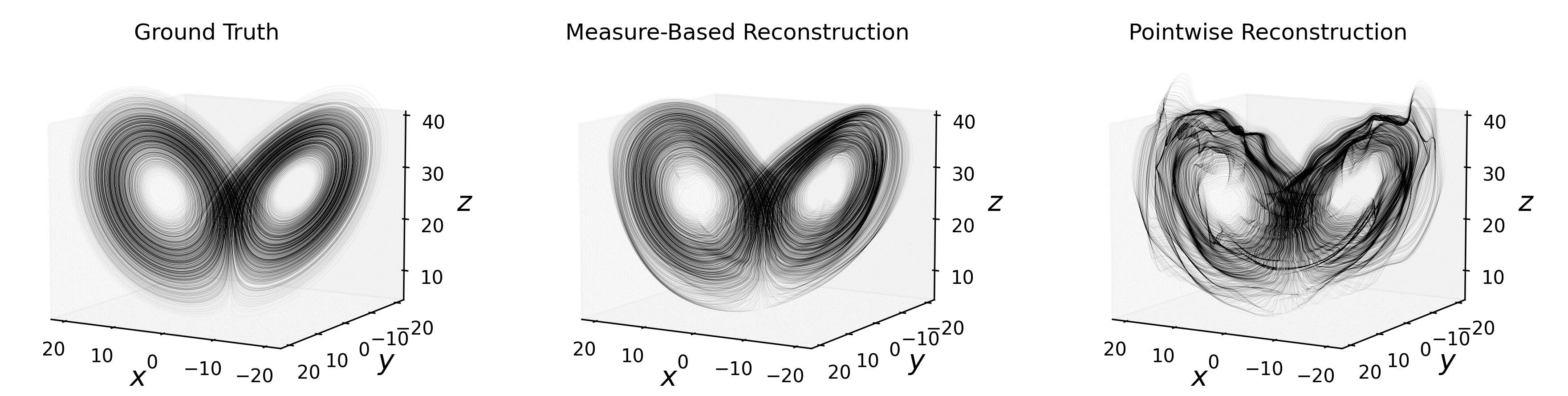
(a)

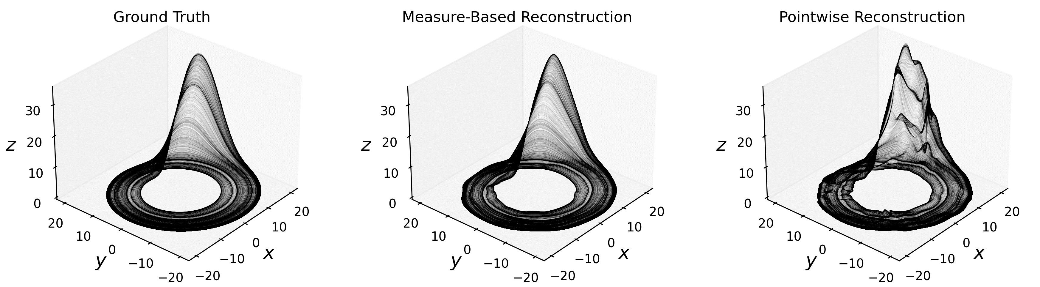
(b)

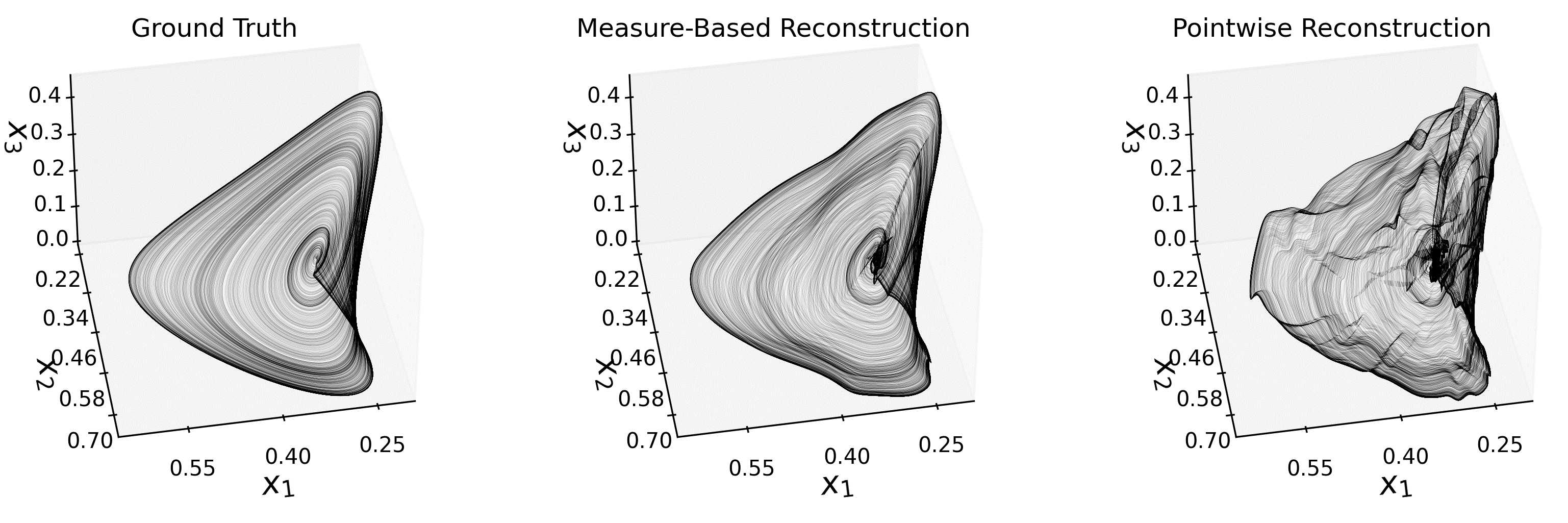
(c)

Figure 2: Visualizations of the learned full-state reconstruction map with sparse and noisy data for systems discussed in Section 4.2. The comparison includes both pointwise and measure-based approaches against the ground truth.

For the experiments shown in Fig. 2, the training data consists of $2\times 10^{3}$ input-output pairs, which are obtained as random samples from a long trajectory. The data is corrupted with i.i.d. extrinsic Gaussian noise samples with covariance matrices $\Sigma_{\texttt{Lorenz}}=0.1I$, $\Sigma_{\texttt{R\"{o}ssler}}=0.1I$, and $\Sigma_{\texttt{Lotka-Volterra}}=5\times 10^{-5}I.$ It is important to note that the noise in the time-delay coordinate may exhibit potential correlations, as the time series used to form these coordinates—taken as the projection of the dynamics onto the $x$-axis—is embedded after the extrinsic noise is applied. The noisy delay state is then partitioned evenly into $20$ cells via a constrained k-means routine [10], from which we then form noisy approximations to the measures following (15). Across all tests, the same four-layer neural network with hyperbolic tangent activation, $100$ nodes in each layer, and a learning rate of $10^{-3}$ is trained for $5\times 10^{4}$ steps. After training the networks on the noisy data, the accuracy of the learned reconstruction map is assessed by applying the network to a clean signal in the time-delay coordinate system. The MSE for the reconstructions visualized in Fig. 2 is summarized in Table 2. For each experiment, the measure-based reconstruction achieves lower error.

4.3 NOAA Sea Surface Temperature Reconstruction

We now consider the problem of reconstructing the NOAA Sea Surface Temperature (SST) from partial measurement data [41]. The SST dataset consists of weekly temperature measurements sampled at a geospatial resolution of $1\degree$; see the supplementary materials for a visualization. Our partial observation of the full SST dataset $\{\mathbf{z}(t_{i})\}\subseteq\mathbb{R}^{44219}$ consists of the temperature time-series $\{x(t_{i})\}\subseteq\mathbb{R}$ recorded at the location $(156\degree,40\degree)$. Our goal is to use the delay state corresponding to $\{x(t_{i})\}$ to learn a reconstruction map for the full state $\{\mathbf{z}(t_{i})\}$. A similar problem is considered in [12, 35].

System	Pointwise MSE	Measure MSE
Lorenz	$7.15\times 10^{-1}$	$2.84\times 10^{-1}$
Rössler	$3.99\times 10^{-1}$	$8.34\times 10^{-2}$
Lotka–Volterra	$2.10\times 10^{-4}$	$9.45\times 10^{-5}$

Table 2: Mean-squared error (MSE) for the reconstructions in Fig. 2. The measure-based reconstruction has lower error for all tests.

The dataset is partitioned into training and testing sets, where the training set contains 355 snapshots ($\approx 5$ years) and the testing set contains 1415 snapshots $(\approx 27$ years). Based on the time-series $\{x(t_{i})\}$, we select a time delay of $\tau=12$ (weeks) and an embedding dimension $m=7$. To reduce the computational cost in learning, similar to [35, 12], we subtract off the temporal mean of the SST dataset and parameterize the full state of the system by the first $N_{\texttt{POD}}$ time-varying POD coefficients, $\{\alpha_{k}(t)\}_{k=1}^{N_{\texttt{POD}}}$, which are obtained via the method of snapshots; see [35, Section 3.1]. That is, we perform the model reduction

$$\mathbf{z}(t_{i})-\overline{\mathbf{z}}=\sum_{k=1}^{N_{\texttt{POD}}}\alpha_{k}(t_{i})\mathbf{m}_{k},\,\,\,\alpha_{k}(t_{i})\in\mathbb{R},\,\,\,\mathbf{m}_{k}\in\mathbb{R}^{44219},$$ (16)

where $\overline{\mathbf{z}}\in\mathbb{R}^{44219}$ is the temporal mean of $\{\mathbf{z}(t_{i})\}$ and $\{\mathbf{m}_{k}\}_{k=1}^{N_{\texttt{POD}}}$ are the first $N_{\texttt{POD}}$ modes. We set $N_{\texttt{POD}}=200$ and aim to learn the POD coefficient reconstruction map $\mathcal{R}_{\theta}:\mathbb{R}^{7}\to\mathbb{R}^{200}$ parameterized by $\theta$, given the paired data

$$\left(x(t_{i}),x(t_{i}-\tau),\dots,x(t_{i}-6\tau)\right)\mapsto\left(\alpha_{1}(t_{i}),\dots\alpha_{200}(t_{i})\right).$$ (17)

For this problem, all training samples are normalized via an affine transformation, such that the $L^{\infty}$ norm of the data vectors is at most 1. We train the neural network parameterization $\mathcal{R}_{\theta}$ using both the pointwise ((13)) and measure-based ((14)) approaches. The pointwise approach seeks to directly enforce the relationship (17) through the mean-squared error, whereas the measure-based approach partitions the delay state into clusters and aims to push forward the empirical measure in each cluster into the corresponding measure in the POD space. We use a constrained k-means routine to evenly partition the delay state into $5$ clusters. A visualization of the 5 clusters can be found in the supplementary materials. We evaluate the performance of the learned reconstruction map by forecasting the time-varying POD coefficients $\{\alpha_{k}(t_{i})\}$ for the testing set, which is then used to reconstruct the full state $\{\mathbf{z}(t_{i})\}$ according to (16).

We note that the challenge of learning the reconstruction map $\mathcal{R}_{\theta}:\mathbb{R}^{7}\to\mathbb{R}^{200}$ is exacerbated by the sparsity of the available training data. Specifically, we aim to learn a $200$-dimensional map using only $355$ training examples. Due to this data sparsity, we utilize MMD based on the Gaussian kernel $k_{\text{g}}(x,y)=\exp(-\|x-y\|_{2}^{2}/2\sigma^{2})$ with $\sigma=3$. The choice of a relatively large $\sigma$ acts as a form of regularization, helping to mitigate overfitting when dealing with sparse samples [18].

	Initial	$10^{3}$ iters	$5\times 10^{3}$ iters	$2\times 10^{4}$ iters
Measure	$13.81\pm 0.98$	$0.72\pm 0.01$	$0.73\pm 0.02$	$0.80\pm 0.02$
Pointwise	$13.95\pm 1.39$	$0.70\pm 0.01$	$0.82\pm 0.01$	$1.31\pm 0.02$

Table 3: Reconstruction mean squared error (MSE) for the SST dataset after various numbers of training iterations. The measure-based approach ((14)) is less prone to overfitting than the pointwise approach ((13)).

In Fig. 3, we visualize the pointwise and measure-based reconstructions of the SST example at testing weeks 425, 550, 675, and 800 after training both models for $25{,}000$ steps. One can observe that the measure-based results align more closely with the ground-truth snapshots, while the pointwise reconstructions exhibit numerous nonphysical oscillations.

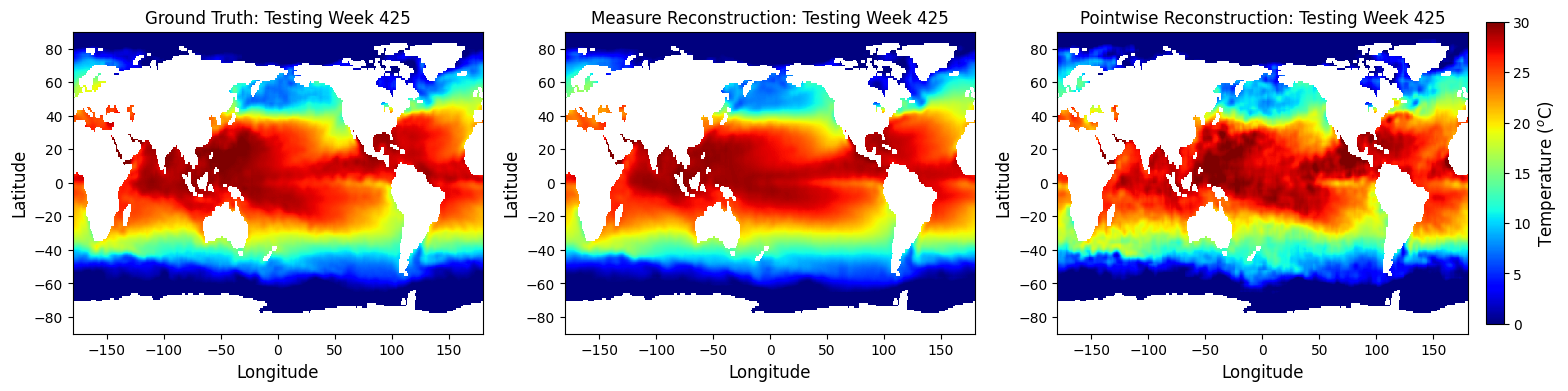
(a)

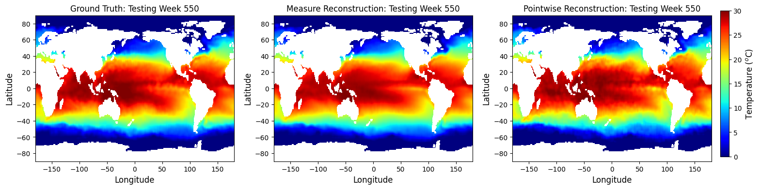
(b)

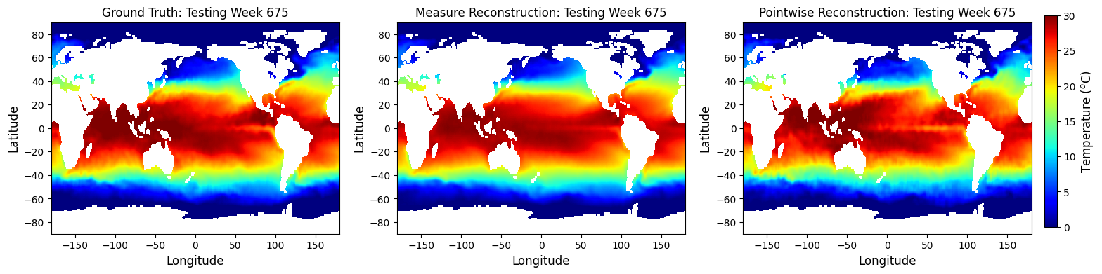
(c)

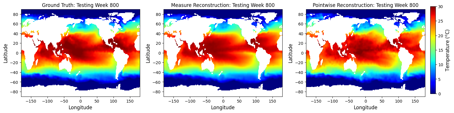
(d)

Figure 3: Visual comparison of the pointwise ((13)) and measure-based ((14)) approaches to reconstructing the SST dataset at the testing weeks 425, 550, 675, and 800. The left column features the ground truth snapshot, the middle column shows the measure-based reconstruction, and the right column shows the pointwise reconstruction.

	Initial	$10^{3}$ iterations	$10^{4}$ iterations	$2\times 10^{4}$ iterations
Gaussian MMD	$158.15\pm 0.27$	$61.04\pm 1.59$	$61.22\pm 0.54$	$67.91\pm 0.49$
Energy MMD	$158.15\pm 0.27$	$49.61\pm 0.48$	$67.85\pm 0.41$	$78.91\pm 0.37$
Pointwise	$158.15\pm 0.27$	$51.00\pm 0.19$	$75.87\pm 0.26$	$84.85\pm 0.25$

Table 4: Testing reconstruction mean squared error (MSE) for the ERA5 wind speed dataset after various iterations during training. For each loss function, the experiment was repeated $5$ times to approximate the mean and standard deviation for the reconstruction error.

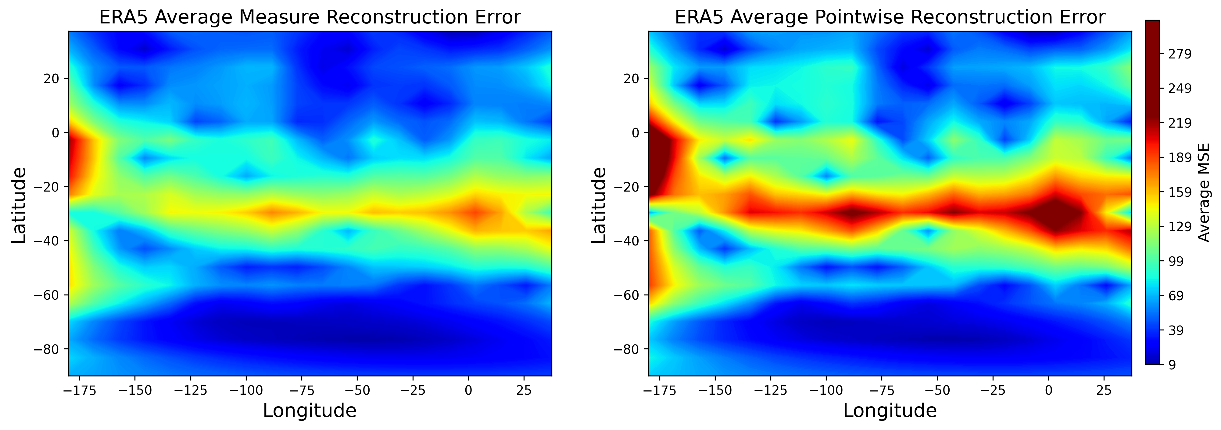
Figure 4: (Left) Spatial distribution of the average MSE for the measure-based reconstruction of the ERA5 dataset, based upon the Gaussian MMD. (Right) Spatial distribution of the average MSE for the pointwise reconstruction of the ERA5 dataset.

In Table 3, we compare the reconstruction errors of the pointwise and measure-based approaches after different numbers of training steps. Due to the sparsity of the training set, the pointwise approach is prone to overfitting, whereas the measure-based relaxation demonstrates greater robustness. After $2\times 10^{4}$ training steps, the reconstruction error for the pointwise approach is approximately $1.6$ times larger than that of the measure-based approach. Both methods train a four-layer fully connected neural network with hyperbolic tangent activation, using the architecture $7\rightarrow 100\rightarrow 100\rightarrow 100\rightarrow 100\rightarrow 200$ and a learning rate of $10^{-3}$. Each neural network is trained $10$ times with different random initializations.

4.4 ERA5 Wind Field Reconstruction

Our final test reconstructs a portion of the ERA5 wind speed dataset using partial measurement data [24]. We consider the ERA5 wind dataset sampled at a geopotential height of Z500, restricted to latitudes between $-180\degree$ and $-105\degree$ and longitudes between $-90\degree$ and $-15\degree$. The dataset is coarsened in both space and time, with measurements taken on approximately a $4\degree$ spatial grid with dimensions $20\times 20$, and separated by $6$ hours in time. For training, we use $2\times 10^{3}$ randomly sampled snapshots of both the $u$ and $v$ wind speed components (longitudinal and latitudinal, respectively) between 2000 and 2007. For testing, we consider the subsequent $5\times 10^{3}$ consecutive snapshots.

While the SST dataset studied in Section 4.3 exhibited strong periodic oscillations with one week between successive snapshots, the ERA5 wind speed dataset is sampled at a sub-daily rate and exhibits complex transient dynamics. Modeling these dynamics using partial observations from a single geospatial location, as done in Section 4.3, is challenging. Similar to [35, 12], we instead use a small number of randomly sampled sensors across the state space to collect partial measurement data. Unlike [35, 12], we also consider time-lagged vectors corresponding to measurements at these spatial locations for performing the full-state reconstruction. This translates the problem of learning the full-state reconstruction map from a scalar-valued time-delayed observable into learning it from a vector-valued time-delayed observable.

More specifically, the task involves learning the state reconstruction map $\mathbf{y}(t_{i})\mapsto\mathbf{z}(t_{i})$, where, for each fixed $t_{i}$, $\mathbf{y}(t_{i})\in\mathbb{R}^{240}$ represents the time-delayed state across all observation locations, and $\mathbf{z}(t_{i})\in\mathbb{R}^{800}$ is the full state of the system. We will now provide a detailed explanation of how the delayed state $\mathbf{y}(t_{i})$ and the full state $\mathbf{z}(t_{i})$ are constructed. The delay state is given by

$$\mathbf{y}(t_{i})=\left(\mathbf{x}(t_{i}),\mathbf{x}(t_{i}-\tau),\dots,\mathbf{x}(t_{i}-(m-1)\tau)\right)\in\mathbb{R}^{60m},$$ (18)

where the vector $\mathbf{x}(t_{i})\in\mathbb{R}^{60}$ represents the ensemble of partial observations at time $t_{i}$, i.e.,

$$\mathbf{x}(t_{i})=\left(u_{n_{1}}(t_{i}),\dots,u_{n_{30}}(t_{i}),v_{n_{1}}(t_{i}),\dots,v_{n_{30}}(t_{i})\right)\in\mathbb{R}^{60}.$$ (19)

In (18), the time-delay and embedding dimension are heuristically chosen as $\tau=6$ (hours) and $m=4$. In (19), the indices $\{n_{k}\}_{k=1}^{30}$ correspond to 30 randomly sampled spatial locations at which we observe the longitudinal and latitudinal components of the wind speed. The full longitudinal wind speed vector is $\mathbf{u}(t_{i})=\left(u_{1}(t_{i}),\dots,u_{400}(t_{i})\right)\in\mathbb{R}^{400}$ representing values at the $20\times 20$ spatial grid, while the full latitudinal wind speed vector is $\mathbf{v}(t_{i})=\left(v_{1}(t_{i}),\dots,v_{400}(t_{i})\right)\in\mathbb{R}^{400}.$ The combined full state can then be written $\mathbf{z}(t_{i})=(\mathbf{u}(t_{i}),\mathbf{v}(t_{i}))\in\mathbb{R}^{800}$, which is precisely the quantity we seek to predict from the delay state $\mathbf{y}(t_{i})$; see (18).

We train models to approximate the state reconstruction map $\mathbf{y}(t_{i})\mapsto\mathbf{z}(t_{i})$ using both the pointwise reconstruction loss ((13)) and the measure-based reconstruction loss ((14)). Throughout, we normalize the training data by subtracting the temporal mean and ensuring that each feature has unit variance. Recall that we randomly sample $2\times 10^{3}$ times $t_{i}$ at which we observe both the delay state $\mathbf{y}(t_{i})$ and the full state $\mathbf{z}(t_{i})$, allowing us to form the paired data $\{(\mathbf{z}(t_{i}),\mathbf{y}(t_{i}))\}_{i=1}^{2000}.$ Thus, when learning the reconstruction map according to the pointwise loss ((13)), we directly enforce the relationship $\mathbf{y}(t_{i})\mapsto\mathbf{z}(t_{i})$, for $1\leq i\leq 2\times 10^{3}$, via the mean squared error.

In contrast, when learning the reconstruction map using the measure-based loss (14), we transform the paired data $\{(\mathbf{z}(t_{i}),\mathbf{y}(t_{i}))\}_{i=1}^{2000}$ into probability measures and aim to find a suitable pushforward map between the probability measures in the time-delayed state space and those in the full state space. We first apply a constrained k-means clustering algorithm to partition the time-delayed samples $\{\mathbf{y}(t_{i})\}_{i=1}^{2000}\subseteq\mathbb{R}^{240}$ into 20 distinct clusters, each containing 100 samples in $\mathbb{R}^{240}$. In doing so, we obtain 20 pairs of probability distributions. During training, we then learn a model that pushes forward each measure in the time-delay coordinate system to the corresponding measure in the full state space. We evaluate the measure-based approach (14) using both the Energy MMD loss (with a polynomial kernel $k_{\text{p}}$) and the Gaussian MMD loss (with a Gaussian kernel $k_{\text{g}}$ and $\sigma=25$).

We train all models using a fully connected neural network with hyperbolic tangent activation function and node sizes $240\rightarrow 500\rightarrow 500\rightarrow 500\rightarrow 800$. We use the Adam optimizer with a learning rate of $10^{-3}$. As shown in Table 4, the pointwise approach has a similar error to the Energy MMD and a lower error than the Gaussian MMD reconstruction after $10^{3}$ training iterations. However, as training continues, the pointwise approach overfits the data, whereas the measure-based approach using both MMD loss functions remains more robust.

It is worth noting that choosing a relatively large bandwidth for the Gaussian MMD acts as additional regularization, helping to prevent overfitting to the locations of the training samples. For longer training times, the Gaussian MMD outperforms the Energy MMD in measure-based reconstruction. The reconstructions based on the Gaussian MMD are smoother than the pointwise reconstructions and more closely match the ground truth; a visualization can be found in the supplementary materials. In Fig. 4, we show the average spatial distribution of the reconstruction error for the Gaussian MMD and pointwise approaches.

5 Conclusion

In this work, we have introduced a significant advancement to the classical Takens’ embedding theorem by developing a measure-theoretic generalization. While the original theory focuses on the embedding property of individual time-delayed trajectories, our novel approach shifts the focus to probability distributions over the state space. Through Corollary 1, our main theoretical contribution, we have demonstrated that the embedding indeed occurs within the space of probability distributions under the pushforward action of the time-delay map. This breakthrough was made possible by integrating the classical Takens’ theorem with cutting-edge tools from optimal transport theory, which were pivotal in our analysis.

Building on these theoretical foundations, we devised a measure-theoretic computational routine for learning the inverse embedding map, also known as the full-state reconstruction map. This innovative method enables the forecasting of an entire high-dimensional dynamical system state from the time lags of a single observable. Our approach involved partitioning the observed trajectory in time-delay coordinates using a k-means clustering routine, where each cluster represents discrete probability measures. During training, we ensured that the corresponding discrete measures in the reconstruction space matched the pushforward distributions of the measures in the time-delay coordinates. This training scheme represents a relaxation of classical pointwise matching, allowing for greater tolerance of pointwise errors in the final reconstruction based on the scale of each discrete measure in the reconstruction space.

While classical pointwise matching may yield more accurate results in the ideal noise-free and densely sampled data scenario, such conditions are rarely met in real-world applications. Our method shines in practical situations where data is often sparse and noisy. Through extensive numerical experiments, ranging from synthetic examples to complex real-world datasets such as NOAA sea-surface temperature and ERA5 wind speed, we have demonstrated the robustness and effectiveness of our approach in learning the reconstruction map under challenging conditions.

This work opens new avenues for future research, where the fusion of measure-theoretic approaches with dynamical systems theory can further enhance our ability to model, predict, and control complex systems in the presence of uncertainty [56, 8, 9, 25, 6]. Our findings not only extend the applicability of Takens’ theorem but also establish a powerful measure-theoretic framework for tackling real-world challenges in data-driven modeling and beyond.

In this supplemental text, we provide additional details to support our theoretical results in Section 3 of the main text, as well as our experimental results in Section 4 of the main text. In Section A, we provide proofs of Proposition 1, Proposition 2, Lemma 1, and Theorem 3. These results are used in the main text to derive Theorem 4 and Corollary 1, which are our paper’s central theoretical results. In Section B, we provide additional information and visualizations for our numerical experiments appearing in Section 4 of the main text.

Appendix A Proofs from Main Text

Proof of Proposition 1.

Let $v=P^{\rho}v+v^{\perp}=v^{\perp}+v^{\top}$ by the unique orthogonal decomposition, where $v^{\perp}\in\text{ker}(P^{\rho})$ and $v^{\top}=P^{\rho}v\in T_{\rho}\mathcal{P}(M)$. Since $v^{\perp}\in\text{ker}(P^{\rho})$,

$$\nabla\cdot(v^{\perp}\rho)=0\implies\ \forall\varsigma\in\mathcal{D}(M):\quad\int_{M}g_{x}(\nabla\varsigma,v^{\perp}){\mathrm{d}}\rho(x)=0.$$ (S1)

Moreover, note that $\varphi\in\mathcal{D}(M)$, so (S1) holds in particular for $\varsigma=\varphi$.

$$\int_{M}g_{x}(\nabla\varphi(x),v){\mathrm{d}}\rho(x) = \int_{M}g_{x}(\nabla\varphi(x),v^{\top}+v^{\perp}){\mathrm{d}}\rho(x)$$

$$= \int_{M}g_{x}(\nabla\varphi(x),P^{\rho}v){\mathrm{d}}\rho(x)+\int_{M}g_{x}(\nabla\varphi(x),v^{\perp}){\mathrm{d}}\rho(x)\,.$$

The last term in the equation above vanishes due to (S1). ∎

Proof of Proposition 2.

Note that for any function $r:M\rightarrow\mathbb{R}$, by definition $\nabla r$ is the vector field in $TM$ such that $g(\nabla r,X)=dr(X)$ , $\forall X\in TM$. We apply this to $r=\varphi\circ f$:

$$g_{x}(\nabla(\varphi\circ f)_{x},X_{x})=d(\varphi\circ f)(X_{x})=d\varphi_{f(x)}(df_{x}X_{x})=d\varphi_{f(x)}Y_{f(x)}\,,$$

where $Y_{f(x)}=df_{x}X_{x}$ is a vector field on $N$. Moreover, since $d\varphi_{f(x)}$ lies in the cotangent bundle on $N$, we have $d\varphi_{y}Y_{y}=q_{y}(\nabla\varphi_{y},Y_{y})$. By plugging this into the equation above with $y=f(x)$, we obtain (9). ∎

Proof of Lemma 1.

Consider that $\rho_{t}$ is an AC curve. Proposition 3 guarantees the existence of a vector field $v_{t}\in L^{2}(M,\rho_{t})$ along $\rho_{t}$ such that the continuity equation holds. However, $v_{t}$ is not necessarily in the tangent space $T_{\rho_{t}}\mathcal{P}(M)\subset L^{2}(M,\rho_{t})$. For an AC curve $\rho_{t}$, we instead define $\frac{d}{dt}\rho_{t}=P^{\rho_{t}}v_{t}\in T_{\rho_{t}}\mathcal{P}(M)$. By the definition of the projection, $\left(\rho_{t},\frac{d}{dt}\rho_{t}\right)$ satisfies the continuity equation. Thus, $\frac{d}{dt}\rho_{t}\in T_{\rho_{t}}\mathcal{P}(M)$ is a tangent vector field along the curve $\rho_{t}$ which proves our result. ∎

Proof of Theorem 3.

We proceed in two steps. First, let $\rho_{t}$ be an AC curve, and $v_{t}=\frac{d}{dt}\rho_{t}$ whose existence is guaranteed by Proposition 3. We then prove that $(F(\rho_{t}),\widetilde{dF}_{\rho_{t}}(v_{t}))$ satisfies the continuity equation and that $\int_{0}^{1}\|\widetilde{dF}_{\rho_{t}}(v_{t})\|_{L^{2}(F(\rho_{t}))}{\mathrm{d}}t<\infty$, which guarantees that $F$ is AC by Proposition 3. Secondly, we extend the previous results to the projected version $dF_{\rho}=P^{F(\rho)}\widetilde{dF_{\rho}}(v)$ which lies in $T_{F(\rho)}\mathcal{P}(N)$ by the definition of the projection operator ((8)).

For the first part, let $\rho_{t}$ be an AC curve in $\mathcal{P}(M)$. Then

$$\int_{0}^{1}\|\widetilde{dF}_{\rho_{t}}(v_{t})\|_{L^{2}(F(\rho_{t}))}\,{\mathrm{d}}t =\int_{0}^{1}\sqrt{\int_{N}q_{y}(\widetilde{dF}_{\rho_{t}}(v_{t})(y)\,,\,\widetilde{dF}_{\rho_{t}}(v_{t})(y))\,{\mathrm{d}}\nu_{t}(y)}\,{\mathrm{d}}t\,,\quad\text{where }\nu_{t}=F(\rho_{t})$$

$$=\int_{0}^{1}\sqrt{\int_{N}q_{y}\big{(}df_{f^{-1}(y)}(v_{t}(f^{-1}(y)))\,,\,df_{f^{-1}(y)}(v_{t}(f^{-1}(y)))\big{)}\,{\mathrm{d}}(f\#\rho_{t})(y)}\,{\mathrm{d}}t$$

$$=\int_{0}^{1}\sqrt{\int_{M}q_{f(x)}(df_{x}(v_{t}(x)),df_{x}(v_{t}(x)))\,{\mathrm{d}}\rho_{t}(x)}\,{\mathrm{d}}t$$

$$\leq\int_{0}^{1}\sqrt{\int_{M}\left(\sup_{x\in M}\|df_{x}\|^{2}\right)g_{x}(v_{t}(x),v_{t}(x))\,{\mathrm{d}}\rho_{t}(x)}\,{\mathrm{d}}t\qquad$$ (S2)

$$=\sup_{x\in M}\|df_{x}\|\int_{0}^{1}\|v_{t}\|_{L^{2}(\rho_{t})}\,{\mathrm{d}}t\,.$$

Since $\sup_{x\in M}\|df_{x}\|<\infty$, the last term is bounded as a result of Proposition 3. The inequality [S2] comes from the definition of the norm $\|df_{x}\|$ and of the supremum:

$$\|df_{x}\|^{2}=\sup_{w\in T_{x}M}\frac{q_{f(x)}(df_{x}w,df_{x}w)}{g_{x}(w,w)}\implies$$

$$\int_{M}q_{f(x)}(df_{x}(v_{t}(x)),df_{x}(v_{t}(x)))\,{\mathrm{d}}\rho_{t}(x)\leq\int_{M}\|df_{x}\|^{2}g_{x}(v_{t}(x),v_{t}(x))\,{\mathrm{d}}\rho_{t}(x)\leq\sup_{x\in M}\|df_{x}\|^{2}\int_{M}g_{x}(v_{t}(x),v_{t}(x))\,{\mathrm{d}}\rho_{t}(x)\,.$$

Next, we show that $(F(\rho_{t}),\widetilde{dF}_{\rho_{t}}(v_{t}))$ satisfies the continuity equation ((5)). For any test function $\varphi\in\mathcal{D}(N\times[0,T])$,

$$\int_{0}^{1}\int_{N}\left(\frac{\partial\varphi}{\partial t}(y)+q_{y}\left(\nabla\varphi(y,t),\widetilde{dF}_{\rho_{t}}(v_{t})(y)\right)\right){\mathrm{d}}\nu_{t}(y){\mathrm{d}}t\,,\quad\nu_{t}=F(\rho_{t})$$ (S3)

$$= \int_{0}^{1}\int_{N}\left(\frac{\partial\varphi}{\partial t}(y,t)+q_{y}(\nabla\varphi(y,t),df_{f^{-1}(y)}\left(v_{t}\left(f^{-1}(y)\right)\right)\right){\mathrm{d}}(f\#\rho_{t})(y){\mathrm{d}}t$$

$$= \int_{0}^{1}\int_{M}\left(\frac{\partial\varphi}{\partial t}(f(x),t)+q_{f(x)}(\nabla\varphi(f(x),t),df_{x}(v_{t}(x)))\right){\mathrm{d}}\rho_{t}(x){\mathrm{d}}t$$

$$= \int_{0}^{1}\int_{M}\left(\frac{\partial\widetilde{\varphi}}{\partial t}(x,t)+g_{x}\left(\nabla\widetilde{\varphi}(x,t),v_{t}(x)\right)\right){\mathrm{d}}\rho_{t}(x){\mathrm{d}}t\,,\quad\widetilde{\varphi}(x,t):=\varphi(f(x),t)\,.$$ (S4)

We used Proposition 2 to obtain (S4). Moreover, note that (S4) is exactly the weak formulation of the continuity equation for $(\rho_{t},v_{t})$ where the test function is $\widetilde{\varphi}$. We now check if $\widetilde{\varphi}\in\mathcal{D}(M\times[0,T])$. Since $f$ is continuously differentiable and $\varphi\in\mathcal{D}(N\times[0,T])$, we have $\widetilde{\varphi}\in\mathcal{C}^{1}(M\times[0,T])$. The support of $\widetilde{\varphi}$ is

$$\text{supp}(\widetilde{\varphi})=\overline{\{(x,t):\varphi((f(x),t))\neq 0\}}\subseteq\overline{(f\otimes\text{{Id}})^{-1}\left(\text{supp}(\varphi)\right)}\,.$$

Since $\text{supp}(\varphi)$ is compact and $(f\otimes\text{{Id}})$ is proper, $(f\otimes\text{{Id}})^{-1}\left(\text{supp}(\varphi)\right)$ is also compact. Moreover, supp$(\widetilde{\varphi})$ is a closed subset of a compact set, and hence itself compact. Thus, $\widetilde{\varphi}\in\mathcal{D}(M\times[0,T])$. Since $(\rho_{t},v_{t})$ satisfies (4) by assumption, (S4) is always zero, which implies that $(F(\rho_{t}),\widetilde{dF}_{\rho_{t}}(v_{t}))$ satisfies the continuity equation ((5)). Finally, we turn to $dF_{\rho_{t}}(v_{t})$.

$$\int_{0}^{1}\int_{N}\left(\frac{\partial\varphi}{\partial t}(y)+q_{y}\left(\nabla\varphi(y,t),dF_{\rho_{t}}(v_{t})(y)\right)\right){\mathrm{d}}\nu_{t}(y){\mathrm{d}}t\,,\quad\nu_{t}=F(\rho_{t})$$

$$= \int_{0}^{1}\int_{N}\frac{\partial\varphi}{\partial t}(y){\mathrm{d}}\nu_{t}(y){\mathrm{d}}t+\int_{0}^{1}\int_{N}q_{y}\left(\nabla\varphi(y,t),P^{F(\rho_{t})}\widetilde{dF}_{\rho_{t}}(v_{t})(y)\right){\mathrm{d}}\nu_{t}(y){\mathrm{d}}t$$

$$= \int_{0}^{1}\int_{N}\frac{\partial\varphi}{\partial t}(y){\mathrm{d}}\nu_{t}(y){\mathrm{d}}t+\int_{0}^{1}\int_{N}q_{y}\big{(}\nabla\varphi(y,t),\widetilde{dF}_{\rho_{t}}(v_{t})(y)\big{)}{\mathrm{d}}\nu_{t}(y){\mathrm{d}}t=0\,,$$

where we used Proposition 1. Thus, $dF_{\rho_{t}}(v_{t})$ also satisfies the continuity equation. ∎

Appendix B Numerical Experiments

B.1 Synthetic Examples

The equations for the dynamical systems studied in Section 4.2 are given by

$$\underbrace{\begin{array}[]{l}\dot{x}_{1}=a_{1}(x_{2}-x_{1})\\ \dot{x}_{2}=x_{1}(a_{2}-x_{3})-x_{2}\\ \dot{x}_{3}=x_{1}x_{2}-a_{3}x_{3}\end{array}}_{\text{Lorenz-63}}\,,\qquad\underbrace{\begin{array}[]{l}\dot{x}_{1}=-x_{2}-x_{3}\\ \dot{x}_{2}=x_{1}+b_{1}x_{2}\\ \dot{x}_{3}=b_{2}+x_{3}(x-b_{3})\end{array}}_{\text{R\"{o}ssler}}\,,\qquad\underbrace{\dot{x}_{i}=r_{i}x_{i}\Bigg{(}1-\sum_{j=1}^{N}\alpha_{ij}x_{j}\Bigg{)}}_{\text{Lotka--Volterra}}.$$

Their parameters are respectively

$$a=\begin{bmatrix}10\\ 28\\ 8/3\end{bmatrix}\,,\qquad b=\begin{bmatrix}0.1\\ 0.1\\ 14\end{bmatrix}\,,\qquad r=\begin{bmatrix}1\\ 0.72\\ 1.53\\ 1.27\end{bmatrix}\,,\qquad\alpha=\begin{bmatrix}1&1.09&1.52&0\\ 0&1&0.44&1.36\\ 2.33&0&1&0.47\\ 1.21&0.51&0.35&1\end{bmatrix},$$

which are standard values known to produce chaotic trajectories. In Section 4.2 of the main text, we compared the pointwise ((13)) and measure-based ((14)) reconstruction schemes for sparse and noisy data coming from these systems.

Here, we show another numerical example, but this time, a large amount of clean, noise-free data is used instead. Figure 1 shows the results in which we perform the full state reconstruction of the same three systems. For this test, we partition the delay state into $100$ cells, which results in $100$ different probability measures for the measure-based loss ((14)). It is worth noting that each measure is an empirical distribution based on thousands of samples. To reduce the computational cost, we used mini-batching to reduce the number of samples in each of the $100$ empirical distributions from $5000$ to $50$. We remark that mini-batch training is not performed in the tests shown in the main text since all examples there are on sparse datasets where the problem instead becomes a lack of data.

After subdividing the training data, we then parameterize $\mathcal{R}_{\theta}$ as a two-layer feed-forward neural network with $100$ nodes in each layer and a hyperbolic tangent activation function. We enforce the distributional loss (14) during training. We use a learning rate of $10^{-3}$. Despite using only $K=100$ measures for learning $\mathcal{R}_{\theta}$, after $100$ epochs of training, we find that the network forecasts the full state of each dynamical system with high-precision. See Figure 5(a) for the Lorenz-63 system, Figure 5(b) for the Rössler system and Figure 5(c) for the Lotka–Volterra system.

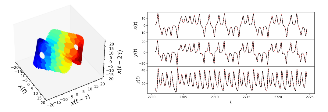
(a)

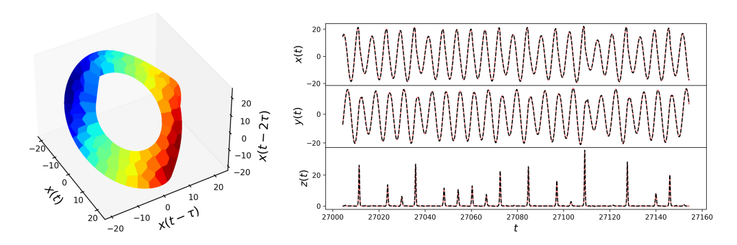
(b)

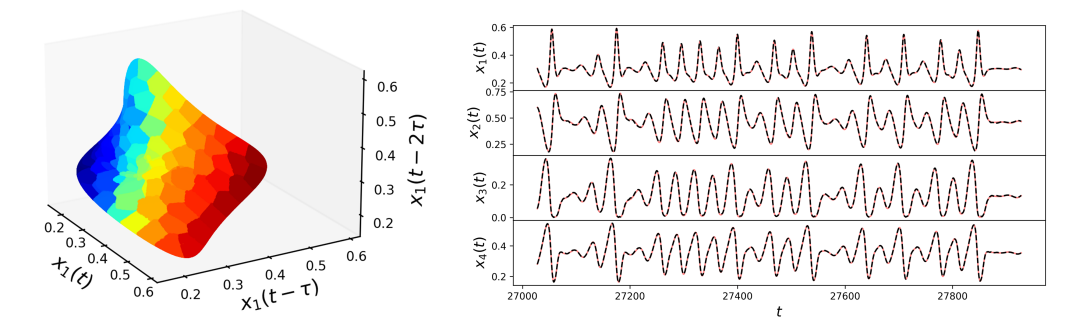
(c)

Figure 5: Learning the full-state reconstruction map for three low-dimensional chaotic attractors. The measures $\Phi\#\mu_{i}$ on the delayed attractor are shown in the left column with each measure colored differently. On the right column, the neural network forecast during testing is shown as the dotted-black line, whereas the ground truth is in red. In this case, the data is noise-free.

B.2 NOAA SST Reconstruction

In Section 4.3, we performed full state reconstruction on the NOAA SST dataset using both the pointwise and measure-based approaches. Figure 6 visualizes the dataset we use to perform the reconstruction. Figure 6(a) shows a single snapshot of the dataset, as well as the geospatial location at which we collect partial observational data. Figure 6(b) plots the temperature time series at this location. Figures 6(c) and 6(d) visualize projections of the input-output measure data used to train the model according to (14). More specifically, Figure 6(d) plots the input measures constructed according to the partially observed data in time-delay coordinates, while 6(c) shows the output measures in the POD reconstruction space.

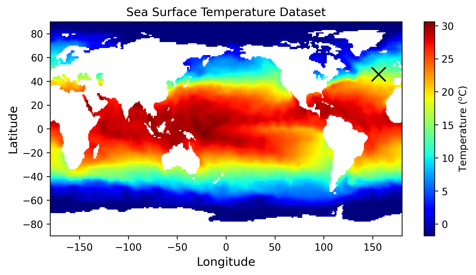
(a)

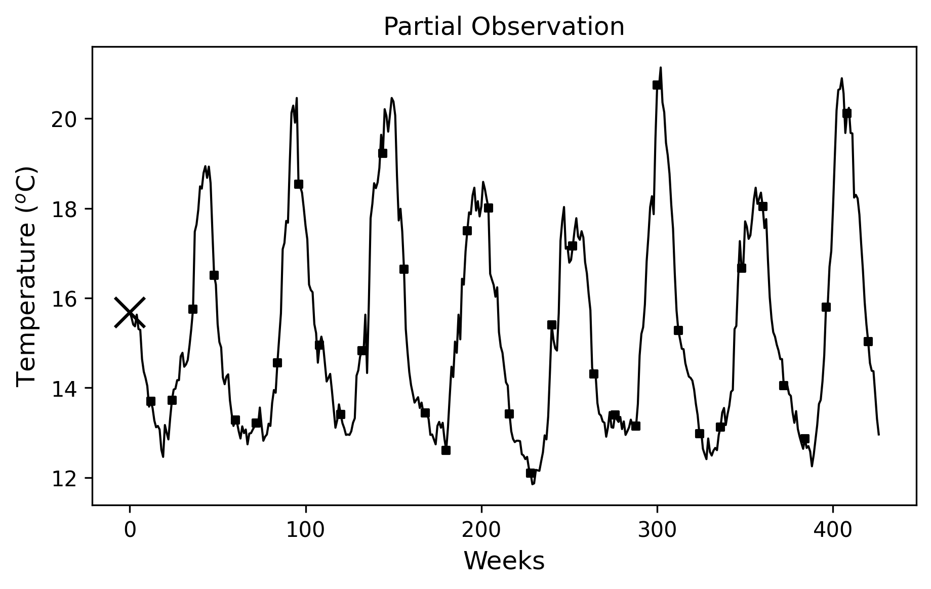
(b)

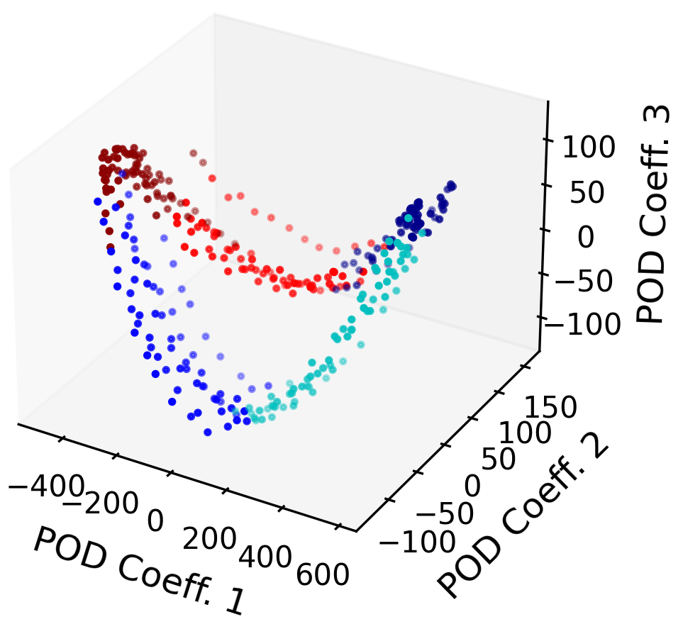
(c)

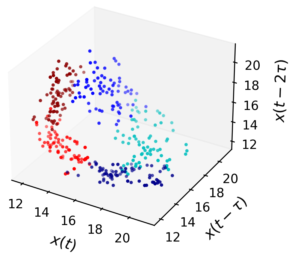
(d)

Figure 6: (a) A single snapshot from the NOAA SST dataset. (b) The time-series from the SST dataset sampled at $(156\degree,40\degree)$, which we regard as our partial observation of the full state. The squares illustrate the time increment of $\tau=12$ which is used to form the delay coordinates. (c) A three-dimensional projection of the POD coefficients $\{\alpha_{k}(t_{i})\}$ which parameterize the full state. (d) A three-dimensional projection of the delayed time-series in (b). The colors in (c) and (d) reflect the five discrete measures which are used to train our measure-based model.

B.3 ERA5 Wind Field Reconstruction

In Section 4.4, we performed full state reconstruction on a portion of the ERA5 wind field dataset. Figure 7 visualizes a single snapshot of the dataset, including the randomly sampled geospatial locations at which we collect partial observational data, as well as an example wind speed time-series at one of these locations. Figure 8 visualizes results for performing the full-state reconstruction on the dataset using both the pointwise ((13)) and measure-based ((14)) approaches.

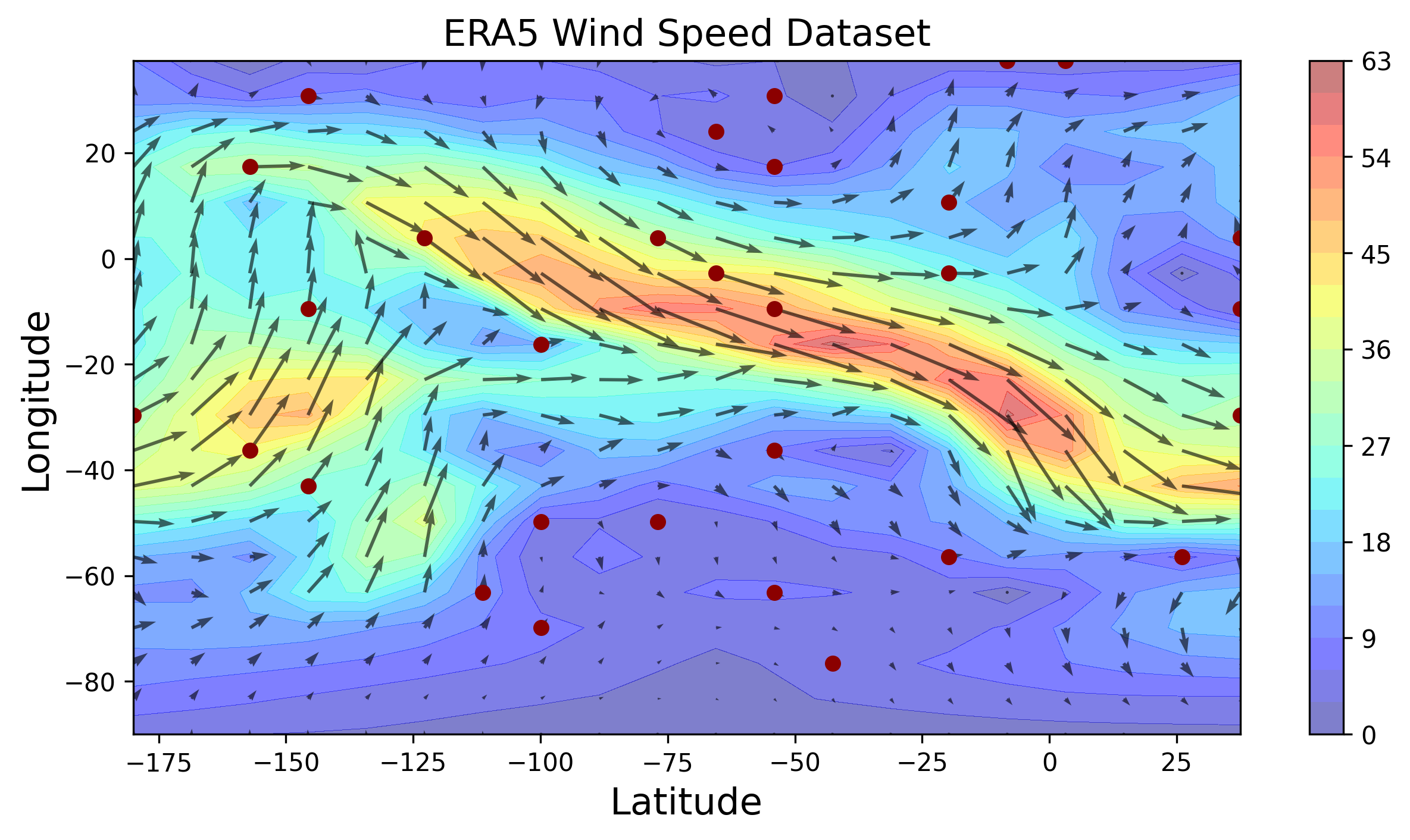
(a)

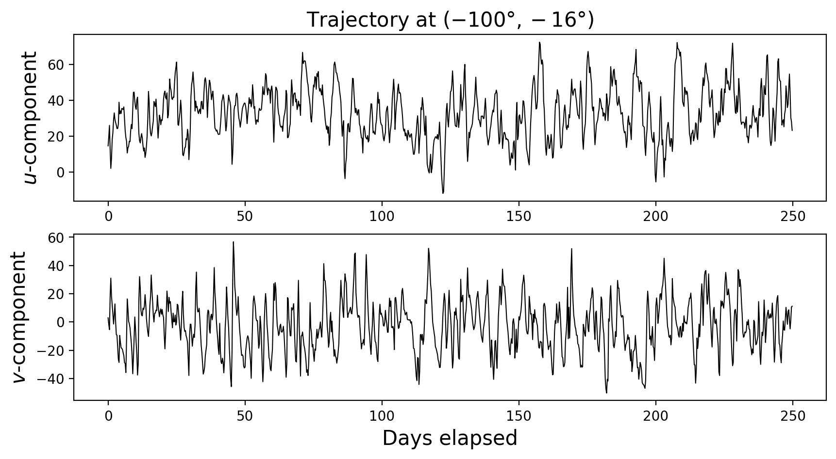
(b)

Figure 7: Visualization of the ERA5 wind speed dataset. (Left) A single snapshot in time of the dataset. The vector field indicates the direction of the wind, the contours illustrate the magnitude of the wind speed, and the 30 red circles show the locations at which we obtain partial observations of the wind field. (Right) The time trajectory corresponding to the geospatial location $(-100\degree,-16\degree)$.

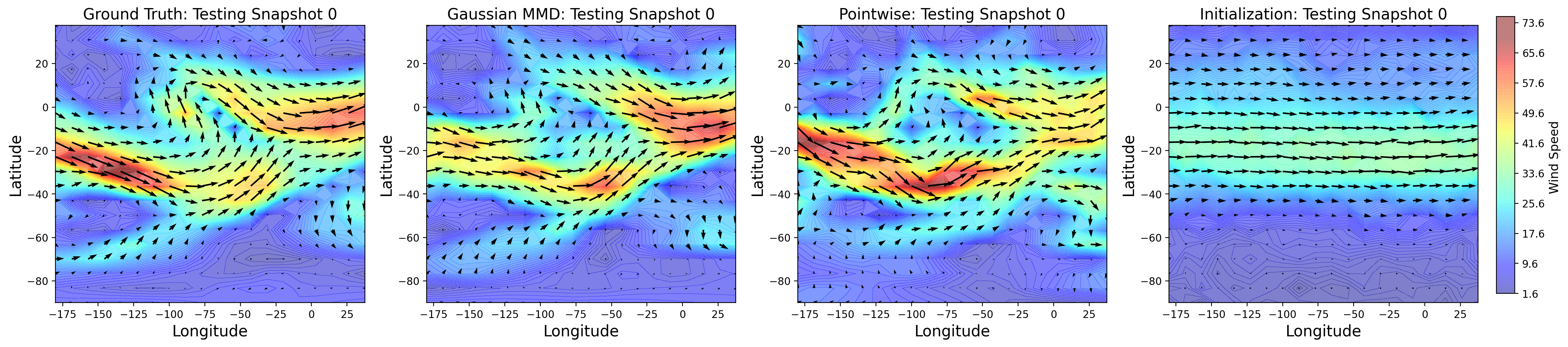
(a)

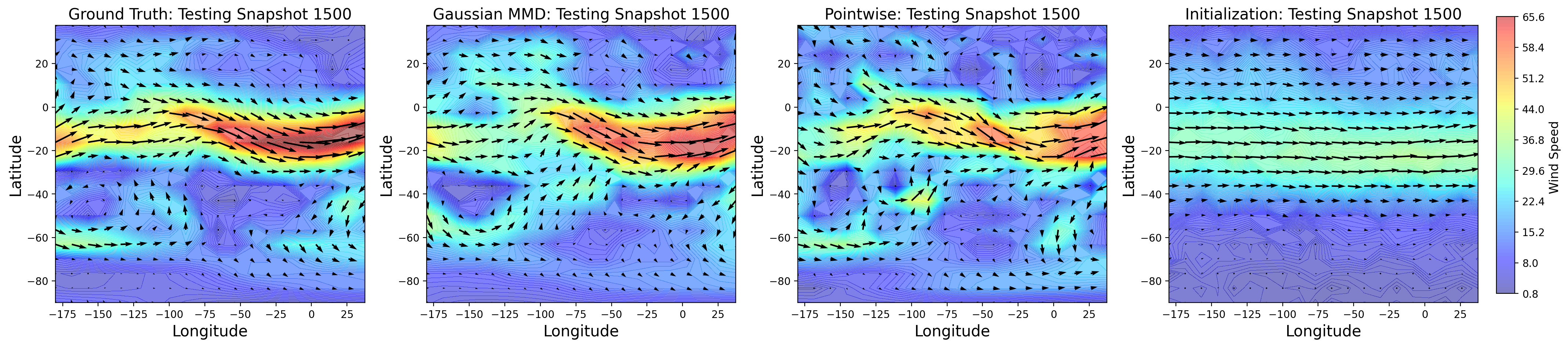
(b)

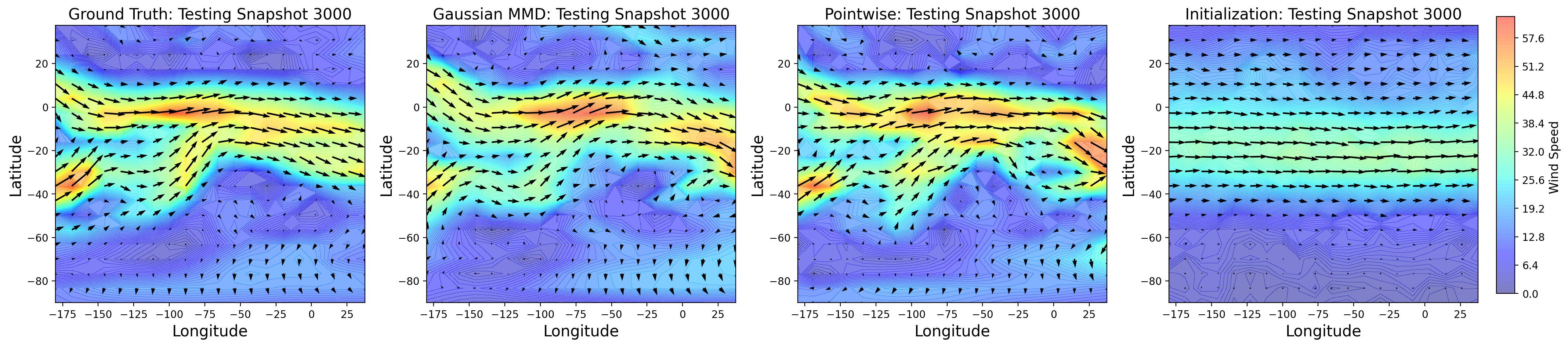
(c)

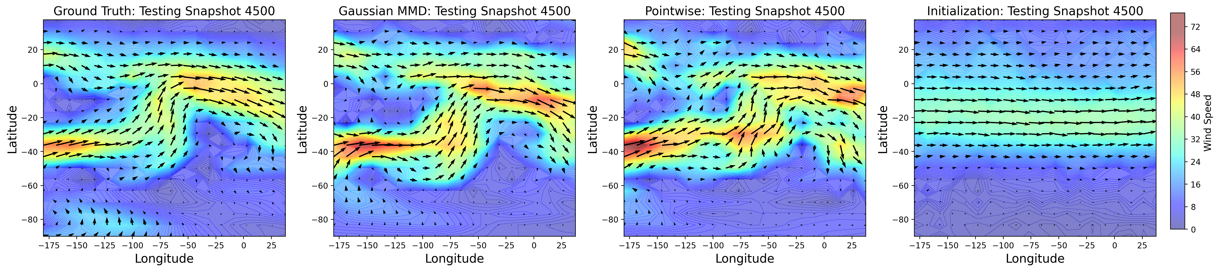
(d)

Figure 8: Visual comparison of the pointwise and measure-based approaches to reconstructing the ERA5 wind dataset after 25000 training iterations. The initialization of the neural networks, shown in the final column, is exactly the same and the only difference among the columns is the loss function used during training.

References

- [1] Luigi Ambrosio, Nicola Gigli, and Giuseppe Savaré. Gradient Flows in Metric Spaces and in the Space of Probability Measures. Birkhäuser Verlag, 2005.
- [2] Roy M Anderson, Christophe Fraser, Azra C Ghani, Christl A Donnelly, Steven Riley, Neil M Ferguson, Gabriel M Leung, Tai H Lam, and Anthony J Hedley. Epidemiology, transmission dynamics and control of SARS: the 2002–2003 epidemic. Philosophical Transactions of the Royal Society of London. Series B: Biological Sciences, 359(1447):1091–1105, 2004.
- [3] Samuel J Araki, Justin W Koo, Robert S Martin, and Ben Dankongkakul. A grid-based nonlinear approach to noise reduction and deconvolution for coupled systems. Physica D: Nonlinear Phenomena, 417:132819, 2021.
- [4] Joseph Bakarji, Kathleen Champion, J Nathan Kutz, and Steven L Brunton. Discovering governing equations from partial measurements with deep delay autoencoders. Proceedings of the Royal Society A, 479(2276):20230422, 2023.
- [5] Krzysztof Barański, Yonatan Gutman, and Adam Śpiewak. A probabilistic Takens theorem. Nonlinearity, 33(9):4940, 2020.
- [6] Florian Beier, Hancheng Bi, Clément Sarrazin, Bernhard Schmitzer, and Gabriele Steidl. Transfer operators from batches of unpaired points via entropic transport kernels. arXiv preprint arXiv:2402.08425, 2024.
- [7] Peter Benner, Serkan Gugercin, and Karen Willcox. A survey of projection-based model reduction methods for parametric dynamical systems. SIAM review, 57(4):483–531, 2015.
- [8] Jonah Botvinick-Greenhouse, Robert Martin, and Yunan Yang. Learning dynamics on invariant measures using PDE-constrained optimization. Chaos: An Interdisciplinary Journal of Nonlinear Science, 33(6), 2023.
- [9] Jonah Botvinick-Greenhouse, Yunan Yang, and Romit Maulik. Generative modeling of time-dependent densities via optimal transport and projection pursuit. Chaos: An Interdisciplinary Journal of Nonlinear Science, 33(10), 2023.
- [10] Paul S Bradley, Kristin P Bennett, and Ayhan Demiriz. Constrained k-means clustering. Microsoft Research, Redmond, 20(0):0, 2000.
- [11] Steven L Brunton, Joshua L Proctor, and J Nathan Kutz. Discovering governing equations from data by sparse identification of nonlinear dynamical systems. Proceedings of the national academy of sciences, 113(15):3932–3937, 2016.
- [12] Jared L Callaham, Kazuki Maeda, and Steven L Brunton. Robust flow reconstruction from limited measurements via sparse representation. Physical Review Fluids, 4(10):103907, 2019.
- [13] Liangyue Cao. Practical method for determining the minimum embedding dimension of a scalar time series. Physica D: Nonlinear Phenomena, 110(1-2):43–50, 1997.
- [14] Martin Casdagli, Stephen Eubank, J Doyne Farmer, and John Gibson. State space reconstruction in the presence of noise. Physica D: Nonlinear Phenomena, 51(1-3):52–98, 1991.
- [15] Björn Engquist, Kui Ren, and Yunan Yang. The quadratic Wasserstein metric for inverse data matching. Inverse Problems, 36(5):055001, 2020.
- [16] Oliver G Ernst, Alois Pichler, and Björn Sprungk. Wasserstein sensitivity of risk and uncertainty propagation. SIAM/ASA Journal on Uncertainty Quantification, 10(3):915–948, 2022.
- [17] J Doyne Farmer and John J Sidorowich. Predicting chaotic time series. Physical review letters, 59(8):845, 1987.
- [18] Jean Feydy. Analyse de données géométriques, au delà des convolutions. PhD thesis, Université Paris-Saclay, 2020.
- [19] Jean Feydy, Thibault Séjourné, François-Xavier Vialard, Shun-ichi Amari, Alain Trouve, and Gabriel Peyré. Interpolating between optimal transport and MMD using Sinkhorn divergences. In The 22nd International Conference on Artificial Intelligence and Statistics, pages 2681–2690, 2019.
- [20] Andrew M Fraser and Harry L Swinney. Independent coordinates for strange attractors from mutual information. Physical review A, 33(2):1134, 1986.
- [21] Michael Ghil and Valerio Lucarini. The physics of climate variability and climate change. Reviews of Modern Physics, 92(3):035002, 2020.
- [22] Peter Grassberger, Rainer Hegger, Holger Kantz, Carsten Schaffrath, and Thomas Schreiber. On noise reduction methods for chaotic data. Chaos: An Interdisciplinary Journal of Nonlinear Science, 3(2):127–141, 1993.
- [23] Arthur Gretton, Karsten M Borgwardt, Malte J Rasch, Bernhard Schölkopf, and Alexander Smola. A kernel two-sample test. The Journal of Machine Learning Research, 13(1):723–773, 2012.
- [24] Hans Hersbach, Bill Bell, Paul Berrisford, Shoji Hirahara, András Horányi, Joaquín Muñoz-Sabater, Julien Nicolas, Carole Peubey, Raluca Radu, Dinand Schepers, et al. The ERA5 global reanalysis. Quarterly Journal of the Royal Meteorological Society, 146(730):1999–2049, 2020.
- [25] Oliver Junge, Daniel Matthes, and Bernhard Schmitzer. Entropic transfer operators. Nonlinearity, 37(6):065004, 2024.
- [26] Omar Khyar and Karam Allali. Global dynamics of a multi-strain SEIR epidemic model with general incidence rates: application to COVID-19 pandemic. Nonlinear dynamics, 102(1):489–509, 2020.
- [27] H_S Kim, R Eykholt, and JD Salas. Nonlinear dynamics, delay times, and embedding windows. Physica D: Nonlinear Phenomena, 127(1-2):48–60, 1999.
- [28] Diederik P Kingma and Jimmy Ba. Adam: A method for stochastic optimization. arXiv preprint arXiv:1412.6980, 2014.
- [29] Aaron Kirtland, Jonah Botvinick-Greenhouse, Marianne DeBrito, Megan Osborne, Casey Johnson, Robert S Martin, Samuel J Araki, and Daniel Q Eckhardt. An unstructured mesh approach to nonlinear noise reduction for coupled systems. SIAM Journal on Applied Dynamical Systems, 22(4):2927–2944, 2023.
- [30] John M. Lee. Introduction to Smooth Manifolds. Springer, 2013.
- [31] Bernadette Lessel and Thomas Schick. Differentiable maps between Wasserstein spaces. arxiv:2010.02131v1, 2020.
- [32] Ambrosio Luigi and Gigli Nicola. A user’s guide to optimal transport. Lecture Notes in Mathematics book series (LNMCIME,volume 2062), 2012.
- [33] James M Lyneis. System dynamics for market forecasting and structural analysis. System Dynamics Review: The Journal of the System Dynamics Society, 16(1):3–25, 2000.
- [34] RS Martin, CM Greve, CE Huerta, AS Wong, JW Koo, and DQ Eckhardt. A robust time-delay selection criterion applied to convergent cross mapping. Chaos: An Interdisciplinary Journal of Nonlinear Science, 34(9), 2024.
- [35] Romit Maulik, Kai Fukami, Nesar Ramachandra, Koji Fukagata, and Kunihiko Taira. Probabilistic neural networks for fluid flow surrogate modeling and data recovery. Physical Review Fluids, 5(10):104401, 2020.
- [36] Audun D Myers, Melih Yesilli, Sarah Tymochko, Firas Khasawneh, and Elizabeth Munch. Teaspoon: A comprehensive python package for topological signal processing. In TDA & Beyond, 2020.
- [37] Gregor Nitsche and Ute Dressler. Controlling chaotic dynamical systems using time delay coordinates. Physica D: Nonlinear Phenomena, 58(1-4):153–164, 1992.
- [38] Louis M Pecora, Linda Moniz, Jonathan Nichols, and Thomas L Carroll. A unified approach to attractor reconstruction. Chaos: An Interdisciplinary Journal of Nonlinear Science, 17(1), 2007.
- [39] Nasim Rahaman, Aristide Baratin, Devansh Arpit, Felix Draxler, Min Lin, Fred Hamprecht, Yoshua Bengio, and Aaron Courville. On the spectral bias of neural networks. In International conference on machine learning, pages 5301–5310. PMLR, 2019.
- [40] Ryan V Raut, Zachary P Rosenthal, Xiaodan Wang, Hanyang Miao, Zhanqi Zhang, Jin-Moo Lee, Marcus E Raichle, Adam Q Bauer, Steven L Brunton, Bingni W Brunton, et al. Arousal as a universal embedding for spatiotemporal brain dynamics. bioRxiv, pages 2023–11, 2023.
- [41] Richard W. Reynolds, Nick A. Rayner, Thomas M. Smith, Diane C. Stokes, and Wanqiu Wang. An improved in situ and satellite SST analysis for climate. Journal of Climate, 15(13):1609 – 1625, 2002.
- [42] Carl Rhodes and Manfred Morari. False-nearest-neighbors algorithm and noise-corrupted time series. Physical Review E, 55(5):6162, 1997.
- [43] Otto E Rössler. An equation for continuous chaos. Physics Letters A, 57(5):397–398, 1976.
- [44] Tim Sauer, James A Yorke, and Martin Casdagli. Embedology. Journal of statistical Physics, 65:579–616, 1991.
- [45] Tapio Schneider, Paul A O’Gorman, and Xavier J Levine. Water vapor and the dynamics of climate changes. Reviews of Geophysics, 48(3), 2010.
- [46] Hal L Smith. An introduction to delay differential equations with applications to the life sciences, volume 57. springer New York, 2011.
- [47] Jaroslav Stark, David S Broomhead, Michael Evan Davies, and J Huke. Takens embedding theorems for forced and stochastic systems. Nonlinear Analysis: Theory, Methods & Applications, 30(8):5303–5314, 1997.
- [48] Jaroslav Stark, David S Broomhead, Michael Evan Davies, and J Huke. Delay embeddings for forced systems. II. Stochastic forcing. Journal of Nonlinear Science, 13:519–577, 2003.
- [49] George Sugihara, Robert May, Hao Ye, Chih-hao Hsieh, Ethan Deyle, Michael Fogarty, and Stephan Munch. Detecting causality in complex ecosystems. science, 338(6106):496–500, 2012.
- [50] Floris Takens. Detecting strange attractors in turbulence. In Dynamical Systems and Turbulence, Warwick 1980, pages 366–381. Springer, 1981.
- [51] Eugene Tan, Shannon Algar, Débora Corrêa, Michael Small, Thomas Stemler, and David Walker. Selecting embedding delays: An overview of embedding techniques and a new method using persistent homology. Chaos: An Interdisciplinary Journal of Nonlinear Science, 33(3), 2023.
- [52] Warwick Tucker. The Lorenz attractor exists. Comptes Rendus de l’Académie des Sciences-Series I-Mathematics, 328(12):1197–1202, 1999.
- [53] JA Vano, JC Wildenberg, MB Anderson, JK Noel, and JC Sprott. Chaos in low-dimensional Lotka–Volterra models of competition. Nonlinearity, 19(10):2391, 2006.
- [54] Cedric Villani. Topics in optimal transportation. American Mathematical Society, 2000.
- [55] Cedric Villani. Optimal transport, old and new. Springer, 2008.
- [56] Yunan Yang, Levon Nurbekyan, Elisa Negrini, Robert Martin, and Mirjeta Pasha. Optimal transport for parameter identification of chaotic dynamics via invariant measures. SIAM Journal on Applied Dynamical Systems, 22(1):269–310, 2023.
- [57] Hao Ye, Ethan R Deyle, Luis J Gilarranz, and George Sugihara. Distinguishing time-delayed causal interactions using convergent cross mapping. Scientific reports, 5(1):14750, 2015.
- [58] Charles D Young and Michael D Graham. Deep learning delay coordinate dynamics for chaotic attractors from partial observable data. Physical Review E, 107(3):034215, 2023.
- [59] Lai-Sang Young. What are SRB measures, and which dynamical systems have them? Journal of statistical physics, 108:733–754, 2002.
Supplemental Materials